Sublinear-time Sampling of Spanning Trees in the Congested Clique

Abstract

We present the first sublinear round algorithm for approximately sampling uniform spanning trees in the CongestedClique model of distributed computing. In particular, our algorithm requires $\tilde{O}(n^{0.658})$ rounds for sampling a spanning tree from a distribution within total variation distance $1/n^{c}$, for arbitrary constant $c>0$, from the uniform distribution. More precisely, our algorithm requires $\tilde{O}(n^{1/2+\alpha})$ rounds, where $O(n^{\alpha})$ is the running time of matrix multiplication in the CongestedClique model, currently at $\alpha=1-2/\omega=0.158$, where $\omega$ is the sequential matrix multiplication time exponent. In a remarkable result, Aldous (SIDM 1990) and Broder (FOCS 1989) showed that the first visit edge to each vertex, excluding the start vertex, during a random walk forms a uniformly chosen spanning tree of the underlying graph. The biggest challenge with the Aldous-Broder algorithm is that it requires a random walk that covers the graph; the expected cover time can be $\Theta(mn)$ for an n-vertex, m-edge graph. We overcome this challenge of having to take a long random walk by using a variety of techniques in the CongestedClique model, including fast matrix multiplication, top-down filling of walk midpoints and compressed representation of midpoint sequences, and the fast computation and use of Schur complement and shortcut graphs.

In addition, we show how to take somewhat shorter random walks even more efficiently in the CongestedClique model. Specifically, we show how to construct length-$\tau$ walks, for $\tau=\Omega(n/\log n)$, in $O\left(\frac{\tau}{n}\log\tau\log n\right)$ rounds and for $\tau=O(n/\log n)$ in $O(\log\tau)$ rounds. This implies an $O(\log^{3}n)$-round algorithm in the CongestedClique model for sampling spanning trees for Erdös–Rényi graphs and regular expander graphs due to the $O(n\log n)$ bound on their cover time. This also implies that polylogarithmic-length walks, which are useful for page rank estimation, can be constructed in $O(\log\log n)$ rounds in the CongestedClique model. These results are obtained by adding a load balancing component to the random walk algorithm of Bahmani, Chakrabarti and Xin (SIGMOD 2011) that uses the “doubling” technique.

1 Introduction

Random spanning trees have been a fascinating area of mathematical study given their close connections to electrical circuits and random walks, dating back to Kirchoff in the 19th century. Of particular interest is the Matrix-Tree theorem; usually credited to Kirchoff, although a more thorough account of its history is described in [45]. This theorem states that the number of spanning trees of any graph can be found by taking the determinant of a minor of the graph Laplacian.

The connections between random walks and random spanning trees extend to efficient algorithms for randomly generating uniform spanning trees of a graph. This began with Aldous[1] and Broder[11] independently discovering that the set of edges used to first visit each vertex during a random walk (except the starting vertex of the walk which can be chosen arbitrarily) form a uniformly chosen spanning tree of the graph. Since the expected time needed to visit every vertex of the graph, the cover time, is known to be $O(mn)$ [2], for an $n$-vertex, $m$-edge graph, this immediately leads to an $O(mn)$ expected time algorithm for uniformly sampling spanning trees of a graph exactly. Wilson found a faster random walk algorithm [61] for sampling spanning trees with an expected runtime of the average hitting time of the graph; however, this algorithm still has an expected $\Theta(mn)$ runtime for the worst graphs. Improvements have been made to the base Aldous-Broder algorithm, albeit we need to settle for approximate rather than exact sampling of uniform spanning trees. In particular, the problem with the algorithm is that while many distinct vertices are visited quickly at the beginning of the random walk, it can take a long time for the last few vertices to be visited. This was addressed by the shortcutting method introduced by Mądry and Kelner [44] and extended by Schild [58]. The result by Schild reduces the runtime to $O(m^{1+o(1)})$, for a graph with $m$ edges. The high level idea of the shortcutting method is that once a part of the graph has been fully visited by a random walk, all future visits to that part of the graph are no longer relevant to the generated spanning tree. Thus, instead of rewalking over parts of the graph that have already been visited, the random walk can take a shortcut, jumping directly to a not yet fully visited part of the graph. Finally, using MCMC rather than random walks, an almost optimal, $O(m\log n)$ time algorithm, for approximately sampling spanning trees in the sequential setting has been shown by Anari, Liu, Gharan, Vinzant, and Vuong [3].

These impressive algorithmic advances for sampling random spanning trees are motivated by several applications of random spanning trees in theoretical computer science, including to graph sparsification [34, 27], breakthroughs in approximation algorithms for the traveling salesman problem [5, 32, 41], and the $k$-edge connected multi-subgraph problem [42].

The focus of this paper is distributed random spanning tree sampling. Specifically, we design our algorithms in the well-known CongestedClique model. This model is a simple, bandwidth-restricted “all-to-all” communication model for distributed computing. A wide variety of classical graph problems, including maximal independent set (MIS) [28, 29], $(\Delta+1)$-coloring [17], ruling set [37, 12], minimum spanning tree (MST) [31, 36, 51, 40, 56], shortest paths [9, 20], minimum cut [30], spanners [55], and triangle detection [19, 14] have been studied in the CongestedClique model. The running times of the fastest algorithms for these problems range from $O(1)$ for MST to $\tilde{O}(n^{0.158})$ for exact triangle counting. Algorithms in the CongestedClique model are often the starting point for algorithms in more realistic “all-to-all” communication models for large-scale cluster computing, such as the $k$-machine model [46], the Map Reduce model [43], and the closely related Massively Parallel Computation (MPC) model [4, 8, 33].

While there is vast literature in distributed computing on finding a feasible solution to constraint satisfaction problems, e.g., finding a maximal independent set, a $(\Delta+1)$-coloring, or a spanning tree, there is relatively limited understanding of sampling from a distribution over the set of feasible solutions. For example, due to a series of papers over the last 2 decades [51, 36, 31, 40], the MST problem can be solved in just $O(1)$ rounds in the CongestedClique model. But as far as we know, there is no work on sampling a random spanning tree in the CongestedClique model.

There has been limited work on sampling combinatorial objects (e.g., colorings, independent sets, spanning trees) in other standard models of distributed computing such as Congest and Local; see [26, 18, 24, 23, 25, 35, 22, 13, 57] for examples. For instance, in [24] the authors present a distributed version of the sequential Metropolis-Hastings algorithm for weighted local constraint satisfaction problems. This is improved in [26] and [22]. Nevertheless, while there has been some work on distributed sampling, there are still a lot of fundamental gaps in our understanding of sampling in distributed settings. This paper aims to fill some of these gaps.

1.1 Our Results

Linear-length walks in polylogarithmic rounds.

The biggest challenge with the Aldous-Broder algorithm is that it requires a random walk that covers the graph; such a walk has, for the worst graphs, expected $\Theta(mn)$ length on an $n$-vertex, $m$-edge graph. A natural approach to efficiently implement the Aldous-Broder algorithm in the CongestedClique model would be to parallelize the random walk construction, by leveraging the model’s bandwidth. There are in fact parallel random walk algorithms in “all-to-all” communication models, designed for page rank estimation [6, 50]. These algorithms use the “doubling” technique, which is a popular technique for designing efficient algorithms in “all-to-all” communication networks [28, 37, 47]. At a high level, the idea is for every vertex $v$ to start an iteration possessing some number of walks of length $\ell$ originating at $v$. During the iteration, pairs of walks are “matched” and stitched together to create random walks of length $2\ell$. In order to construct a length-$L$ random walk, the algorithm of Bahmani, Chakrabarti, and Xin [6] starts with every node $v$ holding $L$ length-1 random walks (i.e., random edges) originating at $v$. To implement the Aldous-Broder algorithm, $L$ needs to be $\Theta(mn)$, but for this setting of $L$ even the first “doubling” iteration is too inefficient. The algorithm of Łącki, Mitrović, Onak and Sankowski [50] suffers from the same bottleneck; in fact, in this algorithm each vertex starts off holding even more length-1 walks initially.

Furthermore, these algorithms [6, 50] may take $\Omega(n)$ rounds for the very first “doubling” iteration, even if we seek to construct a much shorter, e.g., $\Theta(n)$-length, random walk. This is despite the fact that the CongestedClique model has an overall bandwidth of $\Theta(n^{2}\log n)$ bits, the same total bandwidth required by [6] for the first doubling iteration. We present a load balanced version of the “doubling” technique and show how to efficiently construct relatively short random walks in the CongestedClique model. The specific theorem we prove and its consequences are provided below. The most interesting instances of this theorem are walks of length $O(n\cdot\text{poly}(\log n))$, which we can construct in $O(\text{poly}(\log n))$ rounds, and walks of length $O(\text{poly}(\log n))$, which we can construct in $O(\log\log n)$ rounds. As described in [6, 50], walks of length $O(\text{poly}(\log n))$ are of particular interest for approximating page ranks.

Theorem 1.

There is an algorithm for taking a random walk of length $O(\tau)$ in the CongestedClique model that runs in

• $O\left(\frac{\tau}{n}\log\tau\log n\right)$-rounds with high probability for $\tau=\Omega(n/\log n)$

• $O(\log\tau)$-rounds with high probability for $\tau=O(n/\log n)$.

Corollary 1.

For a graph with cover time $\tau$, we can sample a random spanning tree in $\tilde{O}(\tau/n)$ rounds in the CongestedClique model with high probability.

Corollary 2.

We can sample random spanning trees in $O(\log^{4}n)$ rounds with high probability (and in $O(\log^{3}n)$ rounds in expectation) in the CongestedClique model for random Erdös–Rényi graphs $G_{n,p}$ where $p\geq\frac{c\log n}{n}$ for any constant $c>1$, and for $d$-regular expander graphs.

The applications to Erdös–Rényi graphs and to $d$-regular expander graphs follows from the $O(n\log n)$ bound on their cover time [11, 15, 16].

Main result: Sampling random spanning trees in sublinear rounds.

The “doubling” technique, which grows random walks in a bottom up fashion, seems to run into a bandwidth bottleneck for walks longer than $\Theta(n)$. Our main contribution in this paper is to show that the Aldous-Broder random spanning tree algorithm can be implemented in the CongestedClique model in $o(n)$ rounds, using a top down, random walk filling approach. The specific theorem we prove is the following.

Theorem 2.

There is an $\tilde{O}(n^{1/2+\alpha})$ round algorithm in the CongestedClique model for approximately generating a uniform spanning tree of an arbitrary unweighted graph within total variation distance $\epsilon=\Omega(\frac{1}{n^{c_{1}}})$, for an arbitrary constant $c_{1}>0$, from the true uniform distribution, where $O(n^{\alpha})$ is the running time for matrix multiplication in the CongestedClique (currently $\alpha=0.158$).

The top down random walk filling approach seems to be a departure from traditional approaches to constructing random walks in a distributed or parallel setting. We combine this with several other techniques to obtain our result, including fast matrix multiplication in the CongestedClique model, walk truncation to manage bandwidth usage, binary search for truncated walk length, sampling random perfect matchings, and using the Schur complement graph as used in [48, 58] and the short-cutting method of Kelner and Mądry [44]. We overview these techniques in the following subsection.

1.2 Overview of techniques

We first describe, at a high level, a sequential algorithm for random walk sampling, which will serve as our starting point. We will then describe how to adapt this sequential algorithm to the CongestedClique model. However, several challenges arise while porting the sequential algorithm to the distributed setting. In the remainder of the section, we discuss these challenges and the key ideas that we use to address them.

Sequential algorithm. Consider the following sequential algorithm that constructs a random walk across multiple phases. In each phase, a new segment of the walk is sampled and this process is repeated until the full walk is constructed. Within each phase we employ two key ideas that make the algorithm more amenable to efficient implementation in the CongestedClique model: (i) the walk segment constructed in each phase contains $\Theta(\sqrt{n})$ distinct vertices and (ii) the algorithm constructs the relevant walk segment by filling in the walk using a top down approach. In short, given a starting vertex and an ending vertex of a walk, a midpoint is sampled (conditioned on the two endpoints) and then we recurse on the two halves. We give more details on this filling in process in later paragraphs. As we will see shortly, these two ideas allow us to effectively share computation in parallel across multiple machines in the CongestedClique model. We need one additional idea to ensure that the algorithm is efficient. Note that since we are only interested in the first entry edges of the random walk into each vertex, we can skip over vertices visited in previous phases. In order to do this “short cutting” over previously visited vertices, we work with the Schur complement graph [48, 58], combined with the short-cutting technique from Kelner and Mądry [44].

Distributed algorithm. Given the above outline of a sequential sampling algorithm, let us focus on transforming it into a distributed algorithm in the CongestedClique model. Suppose that a leader machine ${\sf M}$ is responsible for maintaining the walk segment constructed in a phase. Further, suppose that just before an iteration of the algorithm, which we refer to as a level, ${\sf M}$ holds a “partial walk” with $O(\sqrt{n})$ distinct vertices and its goal is to insert a midpoint between every consecutive pair of vertices in the walk. Since we are filling in the walk in a top-down manner, by a “partial walk” we mean a sequence of vertices in which each pair of consecutive vertices are the end points of an as-yet-unknown random walk of length $\delta>1$ in the graph $G$. Once midpoints are inserted between consecutive vertices in this partial walk, we get a partial walk that has twice as many vertices, with the consecutive vertices being the end points of an as-yet-unknown length $\delta/2$ random walk in the graph $G$. The midpoints are sampled using pre-computed powers of the transition matrix $\mathbf{P}$ of $G$; specifically, the midpoints at this level are sampled using $\mathbf{P}^{\delta/2}$. These matrix powers are computed using the fast CongestedClique matrix multiplication algorithm in [14]. The fact that the partial walk contains $O(\sqrt{n})$ distinct vertices (even though it can contain many more vertices) implies that there are $O(n)$ distinct start-end pairs into which midpoints need to be inserted. Thus, each start-end pair can be assigned to a distinct machine. However, each start-end pair can appear multiple times in the partial walk and the machine assigned to a particular start-end pair is responsible for generating not just one, but multiple midpoints that then need to be sent back to the leader machine ${\sf M}$ to be stitched into the partial walk. These high-level ideas are illustrated in Figure 1.

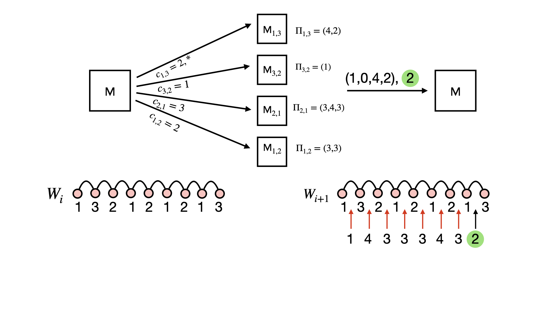
Figure 1: This figure shows the high level process of machine M adding midpoints to the walk $W_{i}$ to obtain $W_{i+1}$. Note that in $W_{i}$ there exist the distinct start-end pairs: $(1,3),(3,2),(2,1),(1,2)$. M sends the count of each start-end pair to the machine responsible for that pair. The machines responsible for each start-end pair then generate a sequence containing the appropriate number of midpoints and then collectively send the multiset of generated midpoints to M. The final midpoint, in green, is sent separately from the multiset and is always placed in the final position. The * indicates that ${\sf M}_{1,3}$ is responsible for the final midpoint. Finally, M samples a perfect matching between the sampled midpoints and spaces in the walk, shown with red arrows. The midpoints are then placed in the walk in these selected indices. This figure ignores the subtlety of ensuring that $W_{i+1}$ contains at most $O(n)$ distinct vertices.

During this process we face two major challenges:

• The algorithm needs to maintain the invariant that the partial walk cannot contain more than $\Theta(\sqrt{n})$ distinct vertices at the end of the level.

• The machine responsible for each start-end pair cannot communicate to machine ${\sf M}$ specific indices (or positions) of the midpoints it generates. This is because even though the partial walk contains only $O(n)$ distinct start-end pairs, a start-end pair may appear as many as $O(n^{3})$ times in the partial walk.

Distributed walk truncation. To address the first obstacle, our algorithm ensures that the leader machine ${\sf M}$ only receives the midpoints up to some truncation point of its partial walk such that the number of distinct vertices within the prefix of the partial walk (up to the truncation point) do not exceed $\Theta(\sqrt{n})$. This seems daunting at first because ${\sf M}$ has to determine a truncation point for the walk without even looking at it. We solve this issue by using distributed binary search. Specifically, ${\sf M}$ guesses a truncation point and distributes requests for midpoint generation for start-end pairs in the partial walk up to the truncation point. We show how machines receiving midpoint generation requests can aggregate their answers efficiently to determine if midpoint generation up to the current truncation point will cause the $\Theta(\sqrt{n})$ budget on the number of distinct vertices in the partial walk to be exceeded. Accordingly ${\sf M}$ can adjust its truncation point guess and this binary search process continues until ${\sf M}$ finds the largest truncation point such that the new partial walk up to that truncation point contains $\Theta(\sqrt{n})$ distinct vertices.

Sampling random perfect matchings. Now, we focus on the second challenge. Once generated, the combined information regarding the identity of the midpoints and their ordering along the walk is prohibitively large to be communicated back to leader machine ${\sf M}$, so we need to compress this data in a way such that ${\sf M}$ will be able to resample the walk locally. Towards this we use the following key ideas: first, ${\sf M}$ only collects a multiset of midpoints, without any information about their position in the walk and secondly, we use a perfect matching sampling algorithm to resample the locations of the midpoints. It is clear that the first idea allows us to save on communication bandwidth. Surprisingly, the compressed information (as multisets) is also sufficient for resampling. Since this is a nontrivial observation, we further expand upon how ${\sf M}$ executes the placement process of collected midpoints. Machine ${\sf M}$ locally constructs a complete bipartite graph, where vertices on one side of the bipartition corresponds to the sampled midpoints and vertices on the other side correspond to positions, identified by start-end pairs, in the walk. We then assign to each edge a weight that corresponds to the probability of that sampled midpoint appearing as a midpoint for that start-end pair and define the weight of a perfect matching as the product of all of its edge weights. Our algorithm then assigns the midpoints to positions in the walk by sampling a random perfect matching with probability proportional to its weight. We show that the leader machine ${\sf M}$ can do this sampling approximately in polynomial time by appealing to the classical results of Jerrum, Sinclair, and Vigoda on approximating the permanent [38] and Jerrum, Valiant, and Vazirani [39] on reducing sampling to counting.

Using Schur complement and short cut graphs. The final piece of our algorithm is the short-cutting process. Recall that the idea is to skip over vertices in each phase that were visited in prior phases. It is evident that short-cutting applies only after the first phase. We use two types of graphs for this – the Schur complement graph and shortcut graph. Consider the situation just before a phase and let $S$ be the set of vertices in the input graph $G$ that have not yet been visited along with the last vertex visited in the previous phase. The Schur complement of $G$, denoted by $\textsc{Schur}(G,S)$, is an edge-weighted, undirected graph with vertex set $S$ such that, roughly speaking, taking a random walk on $\textsc{Schur}(G,S)$ yields the same distribution as taking a random walk on $G$ and then removing the vertices in $V\setminus S$. In essence, $\textsc{Schur}(G,S)$ allows us to take a random walk on $G$ while skipping over vertices in $V\setminus S$. However, the walk on $\textsc{Schur}(G,S)$ returns edges from $\textsc{Schur}(G,S)$. For our spanning tree sampling, we need the first visit edges in the original graph $G$. For this, using ideas from [44], we need another derivative graph on $G$, that we call the shortcut graph. Interestingly, we show that using fast distributed matrix multiplication algorithms, both of these graphs can be computed efficiently in each phase.

1.3 Related Work

In addition to the already discussed work, a few other results are noteworthy in the parallel and distributed settings. Note that Teng [59] showed that in the EREW PRAM model we can take a length $\Theta(n^{3})$ walk, and hence sample a spanning tree, in $O(\log n)$ rounds. In the much weaker Congest model, Sarma, Nanongkai, Pandurangan, and Tetali show that sampling a spanning tree is possible in $\tilde{O}(\sqrt{m}D)$ rounds where $D$ is the diameter of the graph. In this model machines are limited to only sending limited bandwidth messages to their neighbors rather than every machine in the network. Finally, there is a distributed algorithm for estimating the number of spanning trees by Lyons and Gharan [54]. Given the well known reduction from sampling problems to counting problems [39], this may be useful for sampling spanning trees. However, in the case of spanning trees, it is not clear how to parallelize this reduction.

In addition to the doubling results mentioned earlier, one other doubling result of interest is by Luo [53]. However, the result is focused only on sampling the endpoints of random walks, for pagerank, instead of generating the entire walk. Also, the algorithm requires a higher communication bandwidth than our version of the CongestedClique model allows and doesn’t seem to work with long walks.

Another interesting approach to randomly sampling spanning trees is to first randomly sparsify the input graph and then draw a random spanning tree from the sparsified graph. Such an approach in the sequential setting is described by Durfee, Peebles, Peng, and Rao [21]. However, their approach only allows random spanning tree sampling with constant (or slightly sub-constant) total variation distance, whereas our result yields random tree sampling from a distribution with total variation distance $\frac{1}{n^{c_{1}}}$ for any constant $c_{1}>0$ from the uniform distribution. Furthermore, independent of the issue with total variation distance, it is not clear whether their sparsification algorithm can be implemented efficiently in the CongestedClique model.

2 Preliminaries

In this section we describe all the relevant notations and setup that will be used in subsequent sections. The notation $\tilde{O}(f(n))$ refers to $O(f(n)\cdot\text{poly(log(n))})$. We use $G$ to denote the input graph to our algorithm and following convention, $n$ and $m$ will denote the number of vertices and edges in $G$ respectively. We use $\mathbf{P}$ to denote the transition matrix of the random walk on $G$. In particular, any vertex has equal probability of transitioning to any of its neighbors.

2.1 Congested Clique Model

Given an $n$-vertex input graph $G=(V,E)$, the underlying communication network is the size-$n$ clique $K_{n}$, along with a bijection between vertices in $G$ and the machines in the communication network. Thus each machine hosts a distinct vertex and all edges in $G$ incident to that vertex.

Machines have unique IDs of length $O(\log n)$ bits and without loss of generality for our algorithms, we say the machines have IDs $1$ through $n$ and the machine with ID $i$ holds vertex $i$. Computation in the model proceeds in synchronous rounds. Each round begins with each machine performing unbounded local computation. A round then ends with each machine sending a (possibly different) message of length $O(\log n)$ bits to every other machine. Note that a single message is able to encode a constant number of vertices or edges. The time complexity of an algorithm is then measured by the number of rounds used. While machines are theoretically allotted unlimited time for local computation, it is preferred that this time is polynomial in terms of the input graph size. Our algorithms only require polynomial time local computation.

Lenzen [49] proved that in $O(1)$ deterministic rounds it is possible for every vertex to send and receive a total of $O(n)$ messages, regardless of the specific destination of each message. Thus we take the more general view in this model that at each round a machine is able to send and receive a total of $O(n)$ messages instead of placing limits on bandwidth between pairs of machines.

Of particular interest to us is matrix multiplication in the CongestedClique. When $n\times n$ square matrices are distributed amongst machines so that each machine holds one row in each matrix, Censor-Hillel, Kaski, Korhonen, Lenzen, Paz, and Suomela showed that matrix multiplication can be carried out in $O(n^{0.158})$ rounds [14].

2.2 Schur Complement and Shortcut Graphs

We now introduce two derivative graphs of the original graph $G$, called the Schur complement graph and the Shortcut graph. As mentioned earlier, the Schur complement graph will be used to skip over vertices already visited by the random walk constructed in prior phases. The shortcut graph, which is closely related to the Schur complement graph, is used in the setting where we have taken a walk on the Schur complement graph, but we wish to recover the first visit edge of a vertex in the underlying walk in $G$.

Schur complement is a notion from linear algebra that arises during Gaussian elimination. We consider an $n\times n$ matrix $M$ and a subset $S\subset[n]$ of the index set. Let $\overline{S}$ denote $[n]\setminus S$ and, without loss of generality, take $\overline{S}$ to be the first $|\overline{S}|$ indices in $[n]$. Borrowing notation from Section 2.3.3 in [48], we can rewrite $M$ as

$$M=\begin{bmatrix}M_{\overline{S},\overline{S}}&M_{\overline{S},S}\\ M_{S,\overline{S}}&M_{S,S}\end{bmatrix}.$$

When $M_{\overline{S},\overline{S}}$ is invertible, we define the Schur complement of $M$ onto $S$ as

$$\textsc{Schur}(M,S)=M_{SS}-M_{S,\overline{S}}\cdot(M_{\overline{S},\overline{S}})^{-1}\cdot M_{\overline{S},S}.$$

This definition can be ported to graphs by noting that the Schur complement operation is closed for the class of graph Laplacians. Recall that the Laplacian $L(G)$ of a simple, undirected, weighted graph $G=(V,E,w)$ with $V=[n]$ is a $n\times n$ matrix with entries

$$L(G)[i,j]=\begin{cases}\sum_{e:i\in e}w(e),&\text{if }i=j\\ -w(e),&\text{if }i\not=j\text{ and }e=\{i,j\}\in E\\ 0,&\text{otherwise}\end{cases}$$

According to Fact 2.3.6 in [48], for any simple, undirected, weighted graph $G=(V,E,w)$ and vertex subset $S\subset V$, $\textsc{Schur}(L(G),S)$ is itself a Laplacian of a simple, undirected, weighted graph defined on the subset of vertices $S$.

Definition 1 (Schur Complement).

For any simple, undirected, weighted graph $G=(V,E,w)$ and vertex subset $S\subset V$, the Schur complement graph of $G$ onto $S$, denoted $\textsc{Schur}(G,S)$, is the simple, undirected, weighted graph $H$ with vertex set $S$ such that $L(H)=\textsc{Schur}(L(G),S)$.

The motivation for defining $\textsc{Schur}(G,S)$ is that taking a random walk in $G$ starting at $v\in S$ and only looking at the subsequence of visits to vertices in $S$ is identical to taking a random walk in Schur$(G,S)$ starting from the vertex $v\in S$. More precisely, as shown in Theorem 2.4 in [58], the distributions over the sequences of vertices in $S$ generated by the two random walks are identical.

It is also possible to define the graph $\textsc{Schur}(G,S)$ implicitly (and more intuitively) by specifying the transition matrix, $\mathbf{S}$, of a random walk on the graph. Specifically, for any $u,v\in S$, $\mathbf{S}[u,v]$ gives the probability that $v$ is the first vertex in $S\setminus\{u\}$ that a random walk started at $u$ in $G$ visits. Figure 2 provides an illustration of the definition of $\textsc{Schur}(G,S)$.

We now define a second derivative graph, closely related to the Schur complement graph, that we call the shortcut graph. The shortcut graph is used in the setting where we have taken a walk on $\textsc{Schur}(G,S)$, but wish to recover the first visit edge of a vertex in the underlying walk on $G$. It is convenient to define the shortcut graph implicitly by specifying its transition matrix.

Definition 2 (Shortcut Graph).

The shortcut graph, ShortCut$(G,S)$, is a weighted directed graph with vertex set $V$ and transition matrix, $\mathbf{Q}$ (for the random walk on ShortCut$(G,S)$) defined as follows. Consider a random walk on $G$ starting at a vertex $u\in V$: $x_{0}=u,x_{1},x_{2},...$. Let $j=\min\{i>0|x_{i}\in S\}$ be the index of the first vertex in the walk, after $x_{0}$, belonging to $S$. Then $\mathbf{Q}[u,v]=\Pr[x_{j-1}=v]$ is the probability that $v$ appears just before $x_{j}$ in this walk.

Suppose that we have a single random transition in $\textsc{Schur}(G,S)$ from vertex $u\in S$ to vertex $w\in S$. Note that this transition corresponds to a random walk from $u$ to $w$ in $G$. Suppose we wish to recover the edge $(v,w)$ used to visit $w$ in this underlying walk on $G$. The shortcut graph provides a probability distribution over neighbors of $w$, that can be used with Bayes’ rule to sample $v$. Specifically, $\mathbf{Q}[u,v]\cdot\frac{1}{\deg_{S}(v)}$ provides an (unnormalized) distribution over neighbors of $w$ for correctly sampling the edge $(v,w)$. This will be explained in detail in Section 3.2.

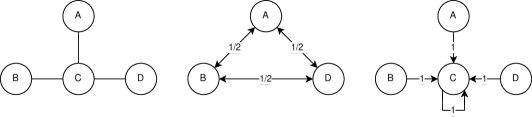
Figure 2: This figure illustrates both derivative graphs of $G$. On the left is the original graph $G$. In this example $S=\{A,B,D\}$. In the center is Schur$(G,S)$. Finally, on the right, is ShortCut$(G,S)$. The labels on the edges give the transition probabilities. Note that the Schur complement graph contains uniform transitions between every vertex. This is because a random walk started at $A$ (for instance) is equally likely to visit $B$ before $D$ or vice versa. In the shortcut graph every vertex always transitions to $C$ since $C$ is always visited directly before a visit to a vertex in $S$ (except possibly at time 0).

2.3 Sampling Weighted Perfect Matchings

We now describe how sampling a weighted matching of a bipartite graph can be achieved in polynomial time. Recall we define the weight of a matching as the product of the weight of its edges. The sum of the weight of every perfect matching is given by the permanent of the biadjacency matrix of the bipartite graph. Jerrum, Sinclair, and Vigoda gave an FPRAS for approximating the permanent [38]. Further, using the sampling to counting reduction of Jerrum, Valiant, and Vazirani [39], we can then approximately sample perfect matchings proportional to their weight. In particular, sampling within total variation $\delta$ can be done with a runtime that is polynomial in both the size of the bipartite graph and $\ln(\frac{1}{\delta})$.

3 Sampling Spanning Trees in Sublinear Rounds

Our algorithm will proceed in phases. In each phase (except possibly the final phase), with high probability, an additional $\Theta(\sqrt{n})$ distinct vertices will compute their first visit edges in the random walk. This leads to a total of $O(\sqrt{n})$ phases being required to generate a uniform spanning tree. We spend (roughly) matrix multiplication time per phase, for a total running time of $\tilde{O}(n^{1/2+\alpha})$ rounds. For simplicity, we will begin by focusing on the first phase; subsequent phases will be described separately. For now, we will also assume that every operation can be carried out with exact numerical precision. We relax this requirement in Section 3.5 and show that each operation can still be carried out with the requisite precision in the CongestedClique.

3.1 Phase 1

Let $\rho:=\lceil\sqrt{n}\rceil$. We will build a random walk that terminates with high probability at the time $T$ where the walk first visits the $\rho$-th distinct vertex. Using the fact that the cover time of any unweighted undirected graph is $O(n^{3}$) and Markov’s inequality, we see that an $O(n^{3})$ length random walk covers the graph with probability at least $\frac{1}{2}$. Thus, for $c_{2}>0$, $T\leq O(n^{3}\log c_{2})$ with probability at least $1-\frac{1}{c_{2}}$. In particular, for later analysis, we choose $c_{2}=\Theta\big{(}n^{1/2+c_{1}}\big{)}$. Initially, we begin generating a walk of target length $\ell:=\Theta(n^{3}\log c_{2})$. We will truncate this walk as needed so that the walk ends at time $T$.

3.1.1 Sequential Random Walk Algorithm

For clarity, we will start by describing a sequential version of the algorithm – which contains some key ideas of our final algorithm – and then show how to implement this efficiently in the CongestedClique. We first ensure that $\ell$ is a power of $2$ by rounding $\ell$ up to the nearest power of $2$. The phase then begins with a Initialization Step, where the transition matrix of the random walk on the graph, $\mathbf{P}$, as well as the matrix powers $\mathbf{P}^{2},\mathbf{P}^{4},\mathbf{P}^{8},...,\mathbf{P}^{\ell}$ are computed.

We now describe the “top down” walk filling process. The initial partial walk $W_{1}$ is generated by first choosing an arbitrary start vertex $w_{0}$. The end vertex, $w_{\ell}$, is sampled with the correct probability, conditioned on $w_{0}$ being the start vertex. In particular, the distribution for $w_{\ell}$ is given by $\mathbf{P}^{\ell}[w_{0},*]$, the row corresponding to vertex $w_{0}$ in $\mathbf{P}^{\ell}$. The walk is then iteratively filled level-by-level in $O(\log\ell)$ levels.

Suppose the levels are labeled $1,2,\ldots,\log_{2}\ell$ and let $W_{i}$ denote the partial walk at the beginning of level $i$. Note that $W_{i}$ is a random walk on the graph with transition matrix $\mathbf{P}^{\ell/2^{i-1}}$. During level $i$, we construct the partial walk $W_{i+1}$ from $W_{i}$, by considering each pair of consecutive vertices in $W_{i}$ in chronological order, and placing a vertex, which we will call a midpoint, between this pair. For example, at the beginning of level $1$, the initial partial walk is $W_{1}=(w_{0},w_{\ell})$. During level $1$, the midpoint $w_{\ell/2}$ is sampled and inserting this leads to the partial walk $W_{2}=(w_{0},w_{\ell/2},w_{\ell})$. During any level, by Bayes’ rule, to choose a midpoint between consecutive vertices $w_{p}$ and $w_{q}$, we sample a vertex $w$ with probability proportional to

$$\mathbf{P}^{(q-p)/2}[w_{p},w]\cdot\mathbf{P}^{(q-p)/2}[w,w_{q}]$$ (1)

Finally, we return $W_{\log_{2}(\ell)+1}$.

Lemma 1.

This sequential algorithm correctly samples a random walk of length $\ell$ beginning at $w_{0}$.

Proof.

We can inductively show that $W_{i}$ is a correct random walk on the graph with transition matrix $\mathbf{P}^{\ell/2^{i-1}}$. The base case, $i=1$, is trivial. The inductive step simply follows from the chain rule of probability and the Markov property of random walks. ∎

3.1.2 Sequential Truncated Random Walk Algorithm

Unfortunately, in the CongestedClique model, we don’t know how to efficiently simulate the previous algorithm once more than $\rho$ distinct vertices are contained in the random walk. Note that with high probability a length $\ell$ walk will contain more than $\rho$ distinct vertices. Instead, we let $\tau$ be the stopping time of the random walk on $G$ that is the minimum of $\ell$ and the time at the first occurrence of the $\rho$-th distinct vertex. Our goal is to sample random walks ending at time $\tau$. The minimum of $\ell$ is included in the definition of $\tau$ to handle the low probability event where fewer than $\rho$ distinct vertices are contained in a random walk of length $\ell$.

We now augment the previous algorithm as follows. Consider level $i$, in which we fill in midpoints in chronological order into the partial walk $W_{i}$, to construct partial walk $W_{i+1}$. As we insert a midpoint $w$ between consecutive vertices $w_{p}$ and $w_{q}$ in $W_{i}$, we check if the partial walk contains at least $\rho$ distinct vertices. If so, we truncate the partial walk to end at the first occurrence of the $\rho$-th distinct vertex and call this truncated partial walk $W_{i+1}$. It is possible that no truncation occurs in a level and $W_{i+1}$ is obtained from $W_{i}$ after all midpoints are filled in. Again, we return $W_{\log_{2}(\ell)+1}$.

Lemma 2.

The sequential truncated random walk algorithm samples a random walk of length $\tau$ beginning at $w_{0}$.

Proof.

By the Markov property of random walks, each truncation will have no impact on the probability of vertices placed before the truncation in future levels. Thus, without changing the result returned by the algorithm, we could choose to defer all truncations of the walk to the end of the algorithm. However, it is easy to see that this is simply generating a walk of length $\ell$ and truncating the walk to end at time $\tau$. ∎

3.1.3 Truncated Walk in the Congested Clique

Now we describe how to implement the sequential truncated random walk algorithm described above in the CongestedClique model.

Initialization Step. We begin with the same Initialization Step as in the sequential algorithm; see the pseudocode below (Algorithm 1). The purpose of the Initialization Step is twofold: (i) for each Machine $i$ to hold row $i$ and column $i$ in each of transition matrices $\mathbf{P},\mathbf{P}^{2},\mathbf{P}^{4},\ldots,\mathbf{P}^{\ell}$ and (ii) to construct the initial walk subsequence $W_{1}=(w_{0},w_{\ell})$.

Algorithm 1 Initialization Step

1:Machine $1$ is designated as the “leader” machine ${\sf M}$; ${\sf M}$ designates the vertex it is hosting (vertex 1) as $w_{0}$, the start of the walk.

2:Using the CongestedClique matrix multiplication algorithm from [14], every Machine $i$ computes rows $\mathbf{P}[i,*],\mathbf{P}^{2}[i,*],\mathbf{P}^{4}[i,*],\ldots,\mathbf{P}^{\ell}[i,*]$.

3:Every Machine $i$ sends $\mathbf{P}^{k}[i,j]$ to machine $j$, for all $j,k$.

4:${\sf M}$ samples $w_{\ell}$ from the distribution given by $\mathbf{P}^{\ell}[1,*]$.

We now describe level $i$ of the midpoint filling in process.

Midpoint Placement Step:

We start with the inductive assumption that ${\sf M}$ holds partial walk $W_{i}$ containing at most $\rho$ distinct vertices.

Midpoint Requests. ${\sf M}$ needs to generate midpoints between consecutive pairs of vertices in $W_{i}$. By Formula 1, the probability distribution of a midpoint vertex only depends on the identities of the vertices it is being placed between and the length of the walk between these vertices. Thus, in a given level, all midpoints being placed between the same start and end vertices are drawn from the same probability distribution. Since $W_{i}$ contains at most $O(\sqrt{n})$ distinct vertices, $W_{i}$ can contain at most $O(n)$ distinct (start, end) pairs. ${\sf M}$ will designate $O(n)$ machines, one for each (start, end) pair that ${\sf M}$ needs to sample midpoints between. Specifically, let the machine assigned the (start, end) pair $(p,q)$ be denoted ${\sf M}_{p,q}$. Furthermore, let $c_{p,q}$ denote the number of occurrences of the (start, end) pairs $(p,q)$ as a pair of consecutive vertices in $W_{i}$. The “leader” machine ${\sf M}$, requests $c_{p,q}$ midpoints from machine ${\sf M}_{p,q}$.

Midpoint Generation. We now look at machine ${\sf M}_{p,q}$ receiving a request for $c_{p,q}$ midpoints. The first task of machine ${\sf M}_{p,q}$ is to acquire the distribution from which to sample the midpoints of (start, end) pair $(p,q)$. Recall that consecutive vertices in $W_{i}$ are at distance $\ell/2^{i-1}$ in the underlying graph $G$; for convenience let $\delta$ denote $\ell/2^{i-1}$. For each vertex $j$, machine ${\sf M}_{p,q}$ sends a request to machine $j$ (i.e., the machine hosting vertex $j$), requesting the (scaled) probability that vertex $j$ is the midpoint of a length $\delta$ walk between $p$ and $q$. Note that by Formula (1) this probability is just $\mathbf{P}^{\delta/2}_{p,j}\mathbf{P}^{\delta/2}_{j,q}$. ${\sf M}_{p,q}$ then uses the implicit normalized probability distribution it received from every other machine to independently sample a sequence of midpoints $\Pi_{p,q}=\pi_{1},\ldots,\pi_{c_{p,q}}$.

Algorithm 2 Midpoint Request and Generation

1:Machine ${\sf M}$ holds the current partial walk $W_{i}=(w_{0},w_{\delta},\ldots,w_{\ell^{\prime}})$.

2:${\sf M}$ counts the number of distinct consecutive pairs $(w_{i\delta},w_{(i+1)\delta})$ in $W_{i}$ and the number of occurrences $c_{p,q}$ of each pair $(p,q)$.

3:${\sf M}$ assigns one machine, ${\sf M}_{p,q}$, to each pair $(p,q)$ and sends ${\sf M}_{p,q}$ the corresponding count $c_{p,q}$.

4:${\sf M}_{p,q}$ requests and receives the probability $\mathbf{P}^{\delta/2}_{p,j}\cdot\mathbf{P}^{\delta/2}_{j,q}$ from each machine $j$ hosting vertex $j$.

5:Machine ${\sf M}_{p,q}$ samples the midpoint sequence $\Pi_{p,q}=\pi_{1},\ldots,\pi_{c_{p,q}}$, where each $\pi_{k}$ is sampled according to the (unnormalized) distribution $\left(\mathbf{P}^{\delta/2}_{p,j}\cdot\mathbf{P}^{\delta/2}_{j,q}\right)_{j=1}^{n}$ that machine ${\sf M}_{p,q}$ received.

Midpoint Placement. Finally, ${\sf M}$ needs to fill in the midpoints in level $i$, thereby constructing partial walk $W_{i+1}$ from $W_{i}$. As we are truncating the walk during some levels, we will let $\ell_{i}$ refer to the target length of $W_{i}$. In our notation, the target length of a partial walk is given by the index of its final element. Recall that $\ell_{1}$, the target length of $W_{1}$, was previously denoted by $\ell$ and it equals $\Theta(n^{3}\log c_{2})$.

Imagine for the moment that ${\sf M}$ magically receives $\Pi_{p,q}$ from each machine ${\sf M}_{p,q}$ and fills in the midpoints of each (start, end) pair $(p,q)$ in $W_{i}$ in the same order as the sequence $\Pi_{p,q}$. Let $t$ be the first index of the $\rho$-th distinct vertex if it exists or otherwise $\ell_{i}$. To faithfully execute the sequential truncated algorithm, we would obtain $W_{i+1}$ by truncating this filled in partial walk to end at index $t$.

Returning to the algorithm, ${\sf M}$ is not aware of $t$ in this magically created random walk, as it does not have direct access to each sequence $\Pi_{p,q}$. However, this $t$ has already been determined. One of the key ideas of our algorithm is that it is still possible for machine ${\sf M}$ to compute $t$ efficiently in the CongestedClique model by using distributed binary search. Once $t$ is found, ${\sf M}$ truncates the partial walk $W_{i}$ to end at time $t$. Then, $W_{i}$ is filled in with midpoints. This completes level $i$ and leads to partial walk $W_{i+1}$. We will see in the proof that even though the midpoints are not placed in the same order as each sequence $\Pi_{p,q}$, a random walk is still correctly sampled.

To simplify the exposition, we first present a subroutine called ${\sf Check}$ that takes an integer $\ell^{\prime}\leq\ell_{i}$ and returns whether $\ell^{\prime}\leq t$. There are two conditions that have to be checked. In the magically filled walk, up to index $\ell^{\prime}$, there can be at most $\rho$ distinct vertices. Furthermore, if there are exactly $\rho$ distinct vertices, the final vertex in the walk must be appearing for the first time in the walk.

Note that ${\sf M}$ can query the vertex at some arbitrary position $j$ in the magical walk in $O(1)$ rounds. Call this vertex $m(j)$. In particular, either position $j$ is already determined for $W_{i}$ or ${\sf M}$ can request $m(j)$ from the machine holding that midpoint. We also let $c_{p,q}(\ell^{\prime})$ be defined identically to $c_{p,q}$ with $W_{i}$ truncated to end at index $\ell^{\prime}$. We include a midpoint in this count even if its endpoint falls past $\ell^{\prime}$. Finally, we define $a(p,q,v,\ell^{\prime})$ as the number of occurrences of $v$ in $\Pi_{p,q}$ up to index $c_{p,q}(\ell^{\prime})$.

Algorithm 3 ${\sf Check}(\ell^{\prime})$

1:Machine ${\sf M}$ sends $c_{p,q}(\ell^{\prime})$ to ${\sf M}_{p,q}$.

2:For every vertex $v$, machine ${\sf M}_{p,q}$ sends $a(p,q,v,\ell^{\prime})$ to machine $v$.

3:For every vertex $v$, machine $v$ sends $a(v,\ell^{\prime})=\sum_{(p,q)}a(p,q,v,\ell^{\prime})$ to ${\sf M}$

4:${\sf M}$ computes $d$, the number of distinct vertices $v$ that are either contained in $W_{i}$ up to index $\ell^{\prime}$ or have $a(v,\ell^{\prime})>0$. $d>\rho$: false

5:${\sf M}$ computes $o$, the number of occurrences of $m(\ell^{\prime})$ in $W_{i}$ plus $a(m(\ell^{\prime}),\ell^{\prime})$

6:$d<\rho\lor o=1$

${\sf M}$ can use the procedure ${\sf Check}$ coupled with binary search to find a value of $\ell^{\prime}$ such that $\ell^{\prime}=t$. We can now truncate $W_{i}$ to end at index $t$. We also know the multiset, $\mathbb{M}$, of midpoints to insert into $W_{i}$ to form $W_{i+1}$. Specifically, the multiplicity of a vertex is given by $a(v,\ell^{\prime})$. However, we do not know which position in the walk each midpoint corresponds to. The key idea of our algorithm is we can add the midpoints in a randomly sampled order, as long as the final midpoint is put in the correct position. Special care is taken for the final midpoint as placing it in a different position may change $t$.

In particular, we want to sample an ordering of the midpoints conditioned on the fact that $\mathbb{M}$ is the chosen multiset of midpoints and the final midpoint is placed last. Recall that finding the final midpoint is easy as we can query $m(j)$ for any $j$. Let $S$ be the set of vertices either contained in $W_{i}$ or $\mathbb{M}$. $M$ receives the submatrix $\mathbf{P}^{\delta/2}_{S}$. Note that this matrix has size $O(n)$, so $M$ can receive it in $O(1)$ rounds.

After placing the final midpoint in the final midpoint position of $W_{i}$, we can think of placing the remaining midpoints as sampling a perfect matching in a weighted complete bipartite graph. Specifically, one set of vertices represents the remaining midpoints and the other set represents the remaining midpoint positions (each one is a start/end) pair. We assign the weight of an edge connecting midpoint $j$ with a pair $(p,q)$ to be $\mathbf{P}^{\delta/2}_{p,j}\mathbf{P}^{\delta/2}_{j,q}$. As described in the introduction, we let the weight of a perfect matching be the product of all of its edge weights and approximately sample a perfect matching proportional to its weight using [38, 39]. We choose the total variation distance error of the sampler to be at most $\frac{\epsilon}{\tilde{O}(\sqrt{n})}$. This perfect matching assigns a position in the walk to each midpoint.

Theorem 3.

The algorithm above generates a random walk beginning at vertex $w_{0}$ and ending at vertex $w_{\tau}$ with total variation distance within $\frac{\epsilon}{2\sqrt{n}}$.

Proof.

Placing the midpoints in walk $W_{i}$ to form walk $W_{i+1}$ can be thought about in three steps. First, the final midpoint, $m_{f}$, is sampled and placed in $W_{i}$. Next, a multiset of the midpoints $\mathbb{M}$ is sampled. Finally, a permutation of the midpoints excluding the final midpoints, $\sigma$, is chosen for placing the remaining midpoints in $W_{i}$. Note that the algorithm chooses $m_{f}$ and $\mathbb{M}$ with the exact correct probability, as the magical walk is a true random walk even if it cannot be collected at machine ${\sf M}$. Now, for a permutation $\sigma$ of $\mathbb{M}\setminus\{m_{f}\}$, $P(\sigma|\mathbb{M},m_{f})$ is proportional to the weight of the equivalent perfect matching. This follows from the Markov property of a random walk as elements already exist in $W_{i}$ separating each midpoint position. Thus if we sampled the perfect matching with no error, the walk would be sampled with no error. Therefore, the error in our algorithm is at most the same error with which we sample perfect matchings multiplied by the number of perfect matchings we sample. This is $O(\log n)$ as it is the number of levels in a phase. ∎

3.1.4 Runtime Analysis for Phase 1

Recall that $\ell$ is $\Theta(n^{3})$. Note that the initial matrix exponentiation can be done, using tabulation, in $\tilde{O}(n^{\alpha})$ rounds. Each machine receiving its column in each of the matrices takes $\tilde{O}(1)$ rounds. Furthermore, each level of the algorithm can be done in $\tilde{O}(1)$ rounds, the only part not taking constant time is the binary search. This leads to a total runtime for the first phase of $\tilde{O}(n^{\alpha})$ rounds.

3.2 Subsequent Phases

We now describe a phase of the algorithm after the initial phase. These later phases will make use of the derivative graphs Schur$(G,S)$ and ShortCut$(G,S)$. In this subsection we assume that the transition matrices of these graphs have already been computed and distributed, with Machine $i$ holding row $i$ and column $i$ of each of these matrices. We describe how to compute these transition matrices in a following subsection.

As in Phase 1, we need to sample the next part of the random walk, visiting the next $\rho=\lceil\sqrt{n}\rceil$ distinct vertices. Let $v_{f}$ be the final vertex visited by the walk of the previous phase. Let ${\sf Old}$ denote the set of vertices visited by the final walk of any previous phase. Let $S=\{v_{f}\}\cup(V\setminus{\sf Old})$ denote the as-yet-unvisited vertices, along with $v_{f}$, which will serve as the starting point of continuation of the walk in this phase. Our goal in this and subsequent phases is to find the first visit edge for all vertices in $S$ except $v_{f}$.

We use the same algorithm as we used for Phase 1, while making sure that we skip over the vertices in ${\sf Old}$. We need to skip vertices in ${\sf Old}$ to ensure we have the network bandwidth to visit $\rho$ distinct new vertices. In order to do this, we repeat the algorithm for Phase 1 on the Schur complement of $G$ with respect to $S$, Schur$(G,S)$ (see Section 2), instead of $G$. This explicitly removes all vertices in ${\sf Old}\setminus\{v_{f}\}$ from the graph, while ensuring that we are taking a random walk that is equivalent to taking a random walk on $G$ skipping over vertices in ${\sf Old}\setminus\{v_{f}\}$. Since the cover time of Schur$(G,S)$, for any $S\subseteq V$, is bounded above by the cover time of $G$, we can (as in Phase 1) start with a partial walk $W_{1}=(w_{0},w_{\ell})$ with target length $\Theta(n^{3})$.

However, taking a random walk on Schur$(G,S)$ does not immediately provide first visit edges in $G$ for the vertices in $S$ visited by the walk. This requires additional work and in particular involves the use of the shortcut graph ShortCut$(G,S)$ (see Section 2). We assume each vertex holds both its row and column in the transition matrix of ShortCut$(G,S)$. Suppose that $w_{i}$ is the first appearance of some vertex $v$ in the random walk. Since the walk in Schur$(G,S)$ corresponds to taking “shortcuts” in the original graph (skipping over vertices in ${\sf Old}\setminus\{v_{f}\}$), we cannot say that the first entrance edge for $v$ is $(w_{i-1},w_{i})$.

We now describe our algorithm for sampling the first incoming edge for $v$ given that the last vertex visited in $S$ was $w_{i-1}$. This sampling can be done by examining the probabilities in ShortCut$(G,S)$. In particular, let $u$ be a neighbor of $v$ in $G$ and $\deg_{S}(u)$ be the number of neighbors of $u$ in the set $S$ in the graph $G$. Then, for all neighbors $u$ of $v$ in $G$, an edge $(u,v)$ is sampled as the first visit edge to $v$ with probability proportional to $\mathbf{Q}[w_{i-1},u]\cdot\frac{1}{\deg_{S}(u)}$. Here $\mathbf{Q}$ is the random walk transition matrix of ShortCut$(G,S)$. The correctness of this expression follows by Bayes’ rule, as $\mathbf{Q}[w_{i-1},u]$ gives the probability that a walk started at $w_{i-1}$ in $G$ visits $u$ immediately before its first visit (at a time greater than zero) to a vertex in $S$ and $\frac{1}{\deg_{S}(u)}$ gives the probability that the vertex in $S$ that is then visited is $v$.

Finding the first visit edges of all vertices visited in this phase, via the sampling method described above, can be implemented in $O(1)$ rounds in the CongestedClique model. See the following psuedocode.

Algorithm 4 Sample first visit edges

1:Machine M obtains walk $W=(w_{0}=v_{f}),w_{1},w_{2},...$ on Schur$(G,S)$ Each distinct vertex $v\neq v_{f}\in W$

2:Machine M finds $i=\min\{j\,|\,w_{j}=v\}$

3:Machine M sends $w_{i-1}$ to machine $v$ Each neighbor $u$ of $v$

4:Machine $v$ requests $\mathbf{Q}[w_{i-1},u]\cdot\frac{1}{\deg_{S}(u)}$ from machine $u$

5:Machine $v$ samples vertex $v$’s first entrance edge $(u,v)$, where $u$ is sampled from the (unnormalized) distribution $\left(\mathbf{Q}[w_{i-1},u]\cdot\frac{1}{\deg_{S}(u)}\right)_{u\in N(v)}$

3.3 Analysis

We haven’t determined the time needed to compute the shortcut and Schur complement graphs yet; however, we will see in Sections 3.4 and 3.5 that it requires $\tilde{O}(n^{\alpha})$ rounds. Altogether, the algorithm leads to a runtime of

$$\tilde{O}(n^{1/2+\alpha})$$

as there are $O(\sqrt{n})$ phases which each take time $\tilde{O}(n^{\alpha})$. Finally, we bound the error between the algorithms sampling distribution and the true uniform distribution.

Theorem 4.

The final spanning tree is drawn with total variation distance at most $\epsilon$ from the uniform distribution.

Proof.

Suppose for the moment that in each phase we generate a truly random walk on the graph Schur$(G,S)$ that ends at the first visit to the $\rho$-th distinct vertex. It is easy to see, by the correctness of the Aldous-Broder algorithm, that we would generate a spanning tree of $G$ sampled uniformly at random.

Now, by the value of $c_{2}$ we chose earlier and the union bound, the random walk fails to visit $\rho$ distinct vertices in any phase with probability at most $\epsilon/2$. Say in this case we simply output an arbitrary spanning tree. Furthermore, in each phase, the perfect matching we sample has total variation distance error at most $\frac{\epsilon}{2\sqrt{n}}$. The total variation distance error of our algorithm then follows by applying the union bound across all phases and adding the two sources of error. ∎

3.4 Computing Schur Complement and Shortcut Graphs

We now demonstrate how to approximately compute the shortcut and Schur complement graphs. In this section we use the term subtractive error to refer to negative additive error to emphasize that each approximation is an under-approximation. We first give a lemma regarding the accuraracy to which we can carry out matrix multiplication.

Lemma 3.

Suppose $M$ is a $n\times n$ transition matrix. Let $k$ be a power of $2$ that is $O(n^{c_{3}})$ for $c_{3}>0$. Let $\beta$ be $\Omega(1/n^{c_{4}})$ for $c_{4}>0$. In the CongestedClique we can compute $M^{k}$ with subtractive error at most $\beta$ in $\tilde{O}(n^{\alpha})$ rounds.

Proof.

Let $M^{\prime}$ be round$(M)$, where round returns the input matrix with each entry truncated after $O(\log\frac{1}{\delta})$ bits. In particular, each entry of round$(M)$ has at most $\delta$ subtractive error over $M$.

We will now define $M^{\prime}(k)$ inductively. Let $M^{\prime}(1)=M^{\prime}$. Further, when $k$ is a power of two, let $M^{\prime}(k)=\textit{round}([M^{\prime}(k/2)]^{2})$. We now analyze the subtractive error, $E(k)$, between $M^{k}$ and $M^{\prime}(k)$. Since the sum of any row is at most $1$ and the sum of any column is at most $n$, $E(1)\leq\delta$ and $E(k)\leq(n+1)E(k/2)+\delta$. Thus $E(k)$ is $O(\delta k^{c\log k})$ for some $c>0$.

The proof now follows by choosing $\delta=\Theta(\frac{\beta}{k^{c\log k}})$ and computing $M^{\prime}(k)$. Using the CongestedClique matrix multiplication algorithm and the fact that each matrix entry requires $O(\log\frac{1}{\delta})=O(\log^{2}(n))$ bits we can compute $M^{\prime}(k)$ in $\tilde{O}(n^{\alpha})$ rounds. ∎

Corollary 3.

Let $S$ be any subset of the vertices of $G$. Let $\beta$ be $\Omega(1/n^{c})$ for $c>0$. In the CongestedClique we can compute ShortCut$(G,S)$ with subtractive error at most $\beta$ in $\tilde{O}(n^{\alpha})$ rounds.

Proof.

Let the transition matrix of the random walk on $G$ be $P$. Let the transition matrix of the random walk on ShortCut$(G,S)$ be $\mathbf{Q}$. We will first construct an auxiliary graph $G^{\prime}$. The vertices of $G^{\prime}$ consist of $L\cup R$, where both $L$ and $R$ contain a new copy of every vertex in $V$. For a vertex $v\in V$, call its copy in $L$, $v^{\prime}$, and call its copy in $R$, $v^{\prime\prime}$. Again we define $G^{\prime}$ by defining the transition probabilities, $R$, of its random walk.

$$\begin{cases}R[u^{\prime\prime},u^{\prime\prime}]=1\\ R[u^{\prime},v^{\prime}]=P[u,v],\,\text{if}\,v^{\prime}\notin S\\ R[u^{\prime},u^{\prime\prime}]=\sum_{v\in S}P[u,v]\end{cases}$$

Now consider $R^{\infty}=\lim_{k\to\infty}R^{k}$. We can see that $\mathbf{Q}[u,v]=R^{\infty}[u^{\prime},v^{\prime\prime}]$. Note that since the cover time of $G$ is $O(n^{3})$, we can get a $\delta$ subtractive approximation of $R^{\infty}$ by choosing $k=O(n^{3}\log\frac{1}{\delta})$. This follows because all the vertices in $R$ are absorbing and in constant units of cover time, with probability at least $1/2$, any vertex in $L$ will have a transition to a vertex in $R$. Now the result follows by combining the approximation of $R^{\infty}$ and Lemma 3 using the triangle inequality. ∎

Corollary 4.

Let $S$ be any subset of the vertices of $G$. Let $\beta$ be $\Omega(1/n^{c_{3}})$ for $c_{3}>0$. In the CongestedClique we can compute Schur$(G,S)$ with subtractive error at most $\beta$ in $\tilde{O}(n^{\alpha})$ rounds. Furthermore, this is also true for Schur$(G,S)^{k}$, where $k$ is a power of $2$ and $k$ is $O(n^{c_{4}})$ for $c_{4}>0$.

Proof.

Let $\mathbf{Q}$ be the transition matrix of ShortCut$(G,S)$. Let $R$ be a transition matrix defined over $V$ as follows.

$$R[u,v]=\begin{cases}1,\,\text{if}\,u=v\land\deg_{S}(u)=0\\ \frac{1}{\deg_{S}(u)},\,\text{if}\,\{u,v\}\in E\land v\in S\\ 0,\,\text{otherwise}\end{cases}$$

Now Schur$(G,S)[u,u]=0$, for all $u$. Otherwise, Schur$(G,S)[u,v]$ is proportional to $(\mathbf{Q}R)[u,v]$, with a different proportionality constant for each row. In particular, we need to multiply each row $u$ by $M_{u}=\frac{1}{1-(\mathbf{Q}R)[u,u]}$. Note that $(\mathbf{Q}R)[u,u]$ is the probability that a random walk in $G$ started at $u$ revisits $u$ before visiting any other vertex in $S$. $M_{u}$ is bounded by a polynomial, $O(n^{c})$ for some $c>0$, by Proposition 2.3 of [52].

The result now follows by simple algebra and the previous corollary and lemma. See the next section for a more complete demonstration on how we can normalize a vector ∎

3.5 Numerical Precision

Finally, we show that the entire algorithm can be carried out with the requisite numerical precision. We analyze the algorithm using approximate probabilities instead of exact probabilities. We will assume that each matrix has been computed with subtractive error at most $\beta$. $\beta$ will be chosen later in the proof and will be large enough such that each entry will fit in $O(1)$, $O(\log n)$ bit, words of the CongestedClique model. Specifically, $\beta$ can be made $\Omega\big{(}\frac{1}{n^{c}}\big{)}$ for some $c>0$. All other computations can then be carried out with full precision.

Theorem 5.

There exists a choice of $\beta$ such that the approximate algorithm runs in $\tilde{O}\big{(}n^{\frac{1}{2}+\alpha}\big{)}$ rounds in the CongestedClique model and draws spanning trees from a distribution with a total variation distance at most $\epsilon$ from the uniform distribution.

Proof.

We will consider four versions of the subroutine for sampling random walks in our algorithm for sampling spanning trees. We can use either the sequential truncated random walk algorithm or the distributed truncated random walk algorithm. Either of these algorithms can be used with exact or approximate probabilities. Using the the FPRAS of [38], we know that we can make the distributions of spanning trees generated using the approximate sequential and approximate distributed random walk algorithms have a total variation distance of at most $\frac{\epsilon}{3}$. Furthermore, we already know that generating spanning trees using the sequential truncated walk algorithm with exact probabilities can give a sample with total variation distance at most $\frac{\epsilon}{3}$. Thus, by three applications of the triangle inequality, it is sufficient to show that for sufficiently small $\beta$, the distributions of trees generated using the sequential truncated random walk algorithms with exact and approximate probabilities also have a total variation distance of at most $\frac{\epsilon}{3}$.

We will use a coupling argument to show that the sequential algorithm using approximate probabilities only has a total variation distance of at most $\frac{\epsilon}{3}$ from the sequential algorithm using exact probabilities. It follows easily from probabilistic coupling, that the total variation distance between the two algorithms outputs is at most the probability that the algorithms make a different decision at some point in their computation, using the same source of randomness. Furthermore, it follows that if the two algorithms are drawing samples from distributions with total variation distance at most $\delta$, they will draw different samples with probability at most $\delta$.

Now inductively suppose that the exact and approximate algorithm have made the same choices so far. Suppose we are sampling a midpoint $b$ between vertices $a$ and $c$. We want to sample $b$ with probability $\frac{P[a,b]P[b,c]}{P^{2}[a,c]}$ for one of the matrices $P$. For now assume that $P^{2}[a,c]>\frac{1}{n^{k_{1}}}$, for a yet to be chosen $k_{1}>0$. The approximate algorithm can compute $P[a,b]P[b,c]$ with subtractive error at most $2\beta$. This gives an unnormalized distribution for choosing the midpoint $b$. Then the normalized distribution has total variation distance error at most

$$\frac{\beta}{\frac{1}{n^{k_{1}}}-2n\beta}$$

The denominator is simply a lower bound on the sum of each term in the unnormalized distribution, and we choose $\beta$ to be small enough such that it is nonnegative. This bound on the total variation distance is also a bound on the probability that the two algorithms will sample different choices of $b$.

Now, as we are choosing $\tilde{O}(n^{3})$ midpoints, we can take the union bound to get the probability that the algorithms ever sample a different midpoint is at most

$$\tilde{O}\bigg{(}{n^{3}\frac{\beta}{\frac{1}{n^{k_{1}}}-2n\beta}}\bigg{)}+\tilde{O}\bigg{(}n^{3}\frac{n}{n^{k_{1}}}\bigg{)}$$

The second term is a bound on the probability that our assumption on $k_{1}$ ever fails. We also have to ensure the algorithms both sample the initial endpoint identically, but this is trivial.

We also have to bound the probability that the first visit edges are sampled differently. We get an expression of a similar form, the only nontrivial fact that we need is that $M_{u}$ is bounded by some polynomial $n^{k_{4}}$, as seen in Corollary 4. Then we get the result we need by choosing $k_{1}$ to be sufficiently large and $\beta$ to be sufficiently small. ∎

4 Fast Random Walk Via Doubling

Bahmani, Chakrabarti, and Xin [6] present an algorithm called Doubling that computes a random walk of length $\tau$ in $O(\log\tau)$ iterations in the Map-Reduce model. In this paper, the Map-Reduce model is specified somewhat abstractly, without an explicit notion of machines, communication bandwidth, etc. As a result, a single iteration (consisting of a Map phase, Shuffle phase, and Reduce phase) in this Map-Reduce model may require $\Omega(n)$ rounds in the CongestedClique model and so using the Doubling algorithm directly in the CongestedClique model is not efficient. In this section we present a “load balanced” version of the Doubling algorithm that can compute a length-$n$ walk in $O(\mbox{poly}\log n)$ rounds in the CongestedClique model.

High-level idea. To compute a length-$\tau$ random walk, the Doubling algorithm starts with each vertex $v$ computing $\tau$ length-1 random walks (i.e., random edges) originating at $v$. At each iteration, walks ending at a node $v$ are merged with walks originating at $v$. This halves the number of walks held by a vertex, while doubling the length of every walk. After $O(\log\tau)$ of these “doubling” iterations, every node $v$ holds a length-$\tau$ random walk originating at vertex $v$. While each walk is a proper random walk, because of how the walks are merged (described in detail below), walks originating at different vertices are not independent. The main challenge for the Doubling algorithm is to implement the merging step efficiently in the CongestedClique model. It turns out that even for relatively short walks, i.e., with $\tau=\Theta(n)$, a faithful implementation of the Doubling algorithm requires $\Omega(n^{2}\log n)$ bits to travel to a particular vertex in a single merging step in the worst case, which requires $\Omega(n)$ rounds in the CongestedClique model. We add a “load balancing” component to each merging step so as to take advantage of the overall $\Theta(n^{2})$ bandwidth of the CongestedClique model. We show that with this “load balancing” step in place, each merging step takes $O(\log n)$ rounds, w.h.p.

Load-balanced Doubling Algorithm. We now describe our algorithm. Consider an iteration of the Doubling algorithm. We assume that just before the start of this iteration, each vertex holds a sequence of $k$ walks of length $\eta$ each. Let $W_{v}^{1},W_{v}^{2},\ldots,W_{v}^{k}$ denote the sequence of $k$ length-$\eta$ walks held by vertex $v$. For any $v$ and $i$, we use $W_{v}^{i}[{\sf end}]$ to denote the ID of the last vertex of the walk, $W_{v}^{i}$.

We further assume that both $k$ and $\eta$ are powers of 2 and $k\cdot\eta$ is the smallest power of 2 that is at least $\tau$. Before the first iteration, $k$ is the smallest power of 2 that is at least $\tau$ and $\eta$ is 1. In each iteration, $k$ halves and $\eta$ doubles.

1. Machine $1$ picks a binary string $s$ of length $O(\log^{2}n)$ uniformly at random and broadcasts $s$ to all other machines. Every machine then uses $s$ to pick a hash function $h_{s}$ from a family of $8c\log n$-wise independent hash functions $\mathcal{H}=\{h:[n]\times[k]\to[n]\}$ for constant $c>1$.

2. For $i=1,\dots,k/2:$ each machine $v$ sends the tuple $(v,i,W_{v}^{i})$ to machine $v^{\prime}=h_{s}(W_{v}^{i}[{\sf end}],k-i)$.

3. For $i=k/2+1,\dots,k:$ each machine $v$ sends the tuple $(v,i,W_{v}^{i})$ to machine $v^{\prime\prime}=h_{s}(\texttt{Id}_{v},i)$.

4. Each machine $w$ receiving two walks $W_{u}^{i}$ and $W_{v}^{j}$, where $W_{u}^{i}[{\sf end}]=\texttt{Id}_{v}$, $1\leq i\leq k/2$, and $i+j=k$ concatenates $W_{u}^{i}$ and $W_{v}^{j}$ and sends the tuple $(i,W_{u}^{i}\circ W_{v}^{j})$ to machine $u$. (Here $W_{u}^{i}\circ W_{v}^{j}$ denotes the concatenation of $W_{u}^{i}$ and $W_{v}^{j}$.)

5. Each machine $v$, on receiving a tuple $(i,W)$, sets $W_{v}^{i}:=W$.

Note that in the above index-based merging scheme (which is due to Bahmani, Chakrabarti, and Xin [6]) a walk $W_{u}^{i}$ for $1\leq i\leq k/2$, that ends at vertex $v$, is merged with a walk, $W_{v}^{k-i}$, originating at $v$. In other words, a walk from the first half of $u$’s sequence of walks is merged with the corresponding walk from the second half of $v$’s sequence of walks. As shown in [6], this index-based merging scheme suffices to guarantee that every walk is indeed a random walk.

For our analysis, we will need the following concentration inequality from Bellare and Rompel[10].

Fact 1 ($t$-wise Concentration Bound).

Let $Y_{1},\dots,Y_{m}$ be $t$-wise independent random variables taking values in $[0,1]$ and $Y=\sum^{m}_{i=1}Y_{i}$ with $\mathbb{E}[Y]=\mu$. Then, for any $a>0$, we have,

$$\Pr\big{[}|Y-\mu|\geq a\big{]}\leq 8\bigg{(}\frac{t\mu+t^{2}}{a^{2}}\bigg{)}^{\frac{t}{2}}.$$

Equipped with the fact above, we prove the following key claim that roughly says that in the load-balanced doubling algorithm each vertex sends and receives $O(k\log n)$ tuples.

Lemma 4.

Let $c>1$ be any constant. Then, in step $2$ and step $3$, in the above algorithm, for any $v\in V$, it holds that:

$$\Pr[\text{Machine }v\text{ receives }\geq 16ck\log n\text{ tuples }]\leq n^{-2c}$$

.

Proof.

In step $2$ and $3$ of the load-balanced algorithm above, a total of at most $nk$ number of tuples are distributed using a $t$-wise hash function among $n$ number of vertices where $t=8c\log n$. Towards proving the claim, fix any machine $v$. We define $Y_{j}$ to be the event that machine $v$ gets the $j$-th tuple for $j=1,2,\dots,nk$. Note that, $\mu:=\mathbb{E}\big{[}\sum Y_{j}\big{]}=nk\cdot\frac{1}{n}=k$. Now we set, $a=k\cdot t=8kc\log n$. Using Fact 1 on these random variables, we get,

$$\Pr[v\text{ receives }\geq 16ck\log n\text{ tuples }] \leq\Pr\big{[}|Y-k|\geq k\cdot t\big{]}$$

$$\leq 8\bigg{(}\frac{t(k+t)}{t^{2}k^{2}}\bigg{)}^{\frac{t}{2}}$$

$$\leq 8\bigg{(}\frac{1}{8ck\log n}+\frac{1}{k^{2}}\bigg{)}^{4c\log n}$$

$$\leq 8\cdot k^{-4c\log n}$$

$$\leq 8\cdot 2^{-4c\log n}=n^{-2c}$$

In the fourth line, we use the crude bound $\bigg{(}\frac{1}{8ck\log n}+\frac{1}{k^{2}}\bigg{)}\leq\frac{1}{k}$ and in the last line, we used the assumption $k\geq 2$.

∎

Now, we are ready to bound the running time of one iteration of the load-balanced doubling algorithm.

Lemma 5.

A single iteration of the Load-balanced Doubling algorithm runs in

• $O\left(\frac{\tau}{n}\log n\right)$ rounds with high probability, if $\tau=\Omega(n/\log n)$.

• $O(1)$ rounds with high probability, if $\tau=O(n/\log n)$.

Proof.

First, note that, each tuple of the form $(\texttt{Id}_{v},i,W_{v}^{i})$, used in our distributed doubling algorithm, requires $O(\eta\log n)$ bits to encode, which is $O(\eta)$ messages. We prove the claim by explicitly computing the number of bits communicated by each machine in each of the step in the algorithm.

• Step 1: Machine 1 sends a randomly sampled string $s$ of size $O(\log^{2}n)$ bits to all the other vertices. This can be completed in 2 rounds of communication.

• Step 2 and 3: Each machine $v$ sends $O(k)$ tuples; so sends $O(k\eta)$ messages. On the reception side, it follows from Lemma 4 that each machine $v\in V$ receives less than $16ck\log n$ tuples with probability $\geq 1-n^{-2c}$. Thus, each machine receives $O(k\eta\log n)$ messages with high probability. Using Lenzen’s routing protocol [49], this communication can be completed in the CongestedClique model in $O\left(\max\left\{\frac{k\eta}{n}\log n,1\right\}\right)$ rounds.

• Step 4: Each machine can only send at most the number of messages they received at the end of the Steps 2 and 3, which is $O(k\eta\log n)$ with high probability. On the other hand, in this step, each machine $v$ receives $k/2$ merged walks of $2\eta$-length. It follows that in Step 4, each machine $v$, receives $O(k\eta)$ messages. Thus, as in Steps 2 and 3, the communication in Step 4 can be completed in the CongestedClique model in $O\left(\max\left\{\frac{k\eta}{n}\log n,1\right\}\right)$ rounds.

Noting that in all iterations of the algorithm, $k\eta=\Theta(\tau)$, we obtain the result. ∎

The following theorem is an immediate consequence of the previous lemma, along with the observation that it takes the Doubling algorithm $O(\log\tau)$ iterations to go from length-1 walks to length-$\tau$ walks.

Theorem 6.

There is an algorithm for taking a random walk of length $O(\tau)$ in the CongestedClique model that runs in

• $O\left(\frac{\tau}{n}\log\tau\log n\right)$-rounds with high probability for $\tau=\Omega(n/\log n)$.

• $O(\log\tau)$-rounds with high probability for $\tau=O(n/\log n)$.

5 Conclusion

Sampling random spanning trees uniformly is a fundamental problem with beautiful mathematical connections to random walks, electrical circuits, and graph Laplacians. The problem also has important applications to graph sparsifiers and serves as the basis for new approximation algorithms. Using the Aldous-Broder algorithm based on random walks, we present the first sublinear round algorithm for approximately sampling uniform spanning trees in the CongestedClique model of distributed computing. In particular, our algorithm requires $\tilde{O}(n^{1/2+\alpha})$ rounds for sampling a spanning tree from a distribution with total variation distance $1/n^{c}$, for arbitrary constant $c>0$, from the uniform distribution. In addition, we show how to take somewhat shorter random walks, even more efficiently in the CongestedClique model, leading to much faster spanning tree sampling algorithms for graphs with small cover times.

We hope that our results and techniques will spark new research on distributed sampling of spanning trees. In the CongestedClique model, it may be worthwhile to seek an algorithm that takes matrix multiplication time. A completely different direction involves implementing the MCMC approach, e.g., using the up-down walk from [3], efficiently in the CongestedClique model. The problem is also poorly understood in other models of distributed computing such as the MPC and Congest models.

References

- [1] David J. Aldous. The random walk construction of uniform spanning trees and uniform labelled trees. SIAM Journal on Discrete Mathematics, 3(4):450–465, 1990.
- [2] Romas Aleliunas, Richard M. Karp, Richard J. Lipton, Laszlo Lovasz, and Charles Rackoff. Random walks, universal traversal sequences, and the complexity of maze problems. In 20th Annual Symposium on Foundations of Computer Science (sfcs 1979), pages 218–223, 1979.
- [3] Nima Anari, Kuikui Liu, Shayan Oveis Gharan, Cynthia Vinzant, and Thuy-Duong Vuong. Log-concave polynomials iv: approximate exchange, tight mixing times, and near-optimal sampling of forests. In Proceedings of the 53rd Annual ACM SIGACT Symposium on Theory of Computing, STOC 2021, page 408–420, New York, NY, USA, 2021. Association for Computing Machinery.
- [4] Alexandr Andoni, Aleksandar Nikolov, Krzysztof Onak, and Grigory Yaroslavtsev. Parallel algorithms for geometric graph problems. In Proceedings of the Forty-Sixth Annual ACM Symposium on Theory of Computing, STOC ’14, page 574–583, New York, NY, USA, 2014. Association for Computing Machinery.
- [5] Arash Asadpour, Michel X. Goemans, Aleksander Mądry, Shayan Oveis Gharan, and Amin Saberi. An olog n/log log n-approximation algorithm for the asymmetric traveling salesman problem. Oper. Res., 65(4):1043–1061, aug 2017.
- [6] Bahman Bahmani, Kaushik Chakrabarti, and Dong Xin. Fast personalized pagerank on mapreduce. In Proceedings of the 2011 ACM SIGMOD International Conference on Management of Data, SIGMOD ’11, page 973–984, New York, NY, USA, 2011. Association for Computing Machinery.
- [7] Greg Barnes and Uriel Feige. Short random walks on graphs. SIAM Journal on Discrete Mathematics, 9(1):19–28, 1996.
- [8] Paul Beame, Paraschos Koutris, and Dan Suciu. Communication steps for parallel query processing. J. ACM, 64(6), oct 2017.
- [9] Ruben Becker, Sebastian Forster, Andreas Karrenbauer, and Christoph Lenzen. Near-optimal approximate shortest paths and transshipment in distributed and streaming models. SIAM Journal on Computing, 50(3):815–856, 2021.
- [10] Mihir Bellare and John Rompel. Randomness-efficient oblivious sampling. In Proceedings 35th Annual Symposium on Foundations of Computer Science, pages 276–287. IEEE, 1994.
- [11] A. Broder. Generating random spanning trees. In 30th Annual Symposium on Foundations of Computer Science, pages 442–447, 1989.
- [12] Mélanie Cambus, Fabian Kuhn, Shreyas Pai, and Jara Uitto. Time and space optimal massively parallel algorithm for the 2-ruling set problem. In Rotem Oshman, editor, 37th International Symposium on Distributed Computing, DISC 2023, October 10-12, 2023, L’Aquila, Italy, volume 281 of LIPIcs, pages 11:1–11:12. Schloss Dagstuhl - Leibniz-Zentrum für Informatik, 2023.
- [13] Charlie Carlson, Daniel Frishberg, and Eric Vigoda. Improved Distributed Algorithms for Random Colorings. In Alysson Bessani, Xavier Défago, Junya Nakamura, Koichi Wada, and Yukiko Yamauchi, editors, 27th International Conference on Principles of Distributed Systems (OPODIS 2023), volume 286 of Leibniz International Proceedings in Informatics (LIPIcs), pages 13:1–13:18, Dagstuhl, Germany, 2024. Schloss Dagstuhl – Leibniz-Zentrum für Informatik.
- [14] Keren Censor-Hillel, Petteri Kaski, Janne H. Korhonen, Christoph Lenzen, Ami Paz, and Jukka Suomela. Algebraic methods in the congested clique. In Proceedings of the 2015 ACM Symposium on Principles of Distributed Computing, PODC ’15, page 143–152, New York, NY, USA, 2015. Association for Computing Machinery.
- [15] A. K. Chandra, P. Raghavan, W. L. Ruzzo, and R. Smolensky. The electrical resistance of a graph captures its commute and cover times. In Proceedings of the Twenty-First Annual ACM Symposium on Theory of Computing, STOC ’89, page 574–586, New York, NY, USA, 1989. Association for Computing Machinery.
- [16] Colin Cooper and Alan Frieze. The cover time of sparse random graphs. Random Struct. Algorithms, 30(1–2):1–16, jan 2007.
- [17] Artur Czumaj, Peter Davies, and Merav Parter. Simple, deterministic, constant-round coloring in the congested clique. In Proceedings of the 39th Symposium on Principles of Distributed Computing, PODC ’20, page 309–318, New York, NY, USA, 2020. Association for Computing Machinery.
- [18] Atish Das Sarma, Danupon Nanongkai, Gopal Pandurangan, and Prasad Tetali. Distributed random walks. J. ACM, 60(1), feb 2013.
- [19] Danny Dolev, Christoph Lenzen, and Shir Peled. “Tri, Tri Again”: Finding Triangles and Small Subgraphs in a Distributed Setting. In Proceedings of the 26th International Symposium on Distributed Computing (DISC), pages 195–209, 2012.
- [20] Michal Dory and Merav Parter. Exponentially faster shortest paths in the congested clique. J. ACM, 69(4), aug 2022.
- [21] David Durfee, John Peebles, Richard Peng, and Anup B. Rao. Determinant-preserving sparsification of sddm matrices with applications to counting and sampling spanning trees, 2017.
- [22] Weiming Feng, Thomas P. Hayes, and Yitong Yin. Distributed symmetry breaking in sampling (optimal distributed randomly coloring with fewer colors), 2018.
- [23] Weiming Feng, Thomas P. Hayes, and Yitong Yin. Distributed metropolis sampler with optimal parallelism. In Proceedings of the Thirty-Second Annual ACM-SIAM Symposium on Discrete Algorithms, SODA ’21, page 2121–2140, USA, 2021. Society for Industrial and Applied Mathematics.
- [24] Weiming Feng, Yuxin Sun, and Yitong Yin. What can be sampled locally? In Proceedings of the ACM Symposium on Principles of Distributed Computing, PODC ’17, page 121–130, New York, NY, USA, 2017. Association for Computing Machinery.
- [25] Weiming Feng and Yitong Yin. On local distributed sampling and counting. In Proceedings of the 2018 ACM Symposium on Principles of Distributed Computing, PODC ’18, page 189–198, New York, NY, USA, 2018. Association for Computing Machinery.
- [26] Manuela Fischer and Mohsen Ghaffari. A simple parallel and distributed sampling technique: Local glauber dynamics. In Ulrich Schmid and Josef Widder, editors, 32nd International Symposium on Distributed Computing, DISC 2018, New Orleans, LA, USA, October 15-19, 2018, volume 121 of LIPIcs, pages 26:1–26:11. Schloss Dagstuhl - Leibniz-Zentrum für Informatik, 2018.
- [27] Wai Shing Fung, Ramesh Hariharan, Nicholas J.A. Harvey, and Debmalya Panigrahi. A general framework for graph sparsification. In Proceedings of the Forty-Third Annual ACM Symposium on Theory of Computing, STOC ’11, page 71–80, New York, NY, USA, 2011. Association for Computing Machinery.
- [28] Mohsen Ghaffari. Distributed MIS via all-to-all communication. In Proceedings of the ACM Symposium on Principles of Distributed Computing, PODC 2017, Washington, DC, USA, July 25-27, 2017, pages 141–149, 2017.
- [29] Mohsen Ghaffari, Themis Gouleakis, Christian Konrad, Slobodan Mitrovic, and Ronitt Rubinfeld. Improved massively parallel computation algorithms for mis, matching, and vertex cover. In Proceedings of the 2018 ACM Symposium on Principles of Distributed Computing, PODC 2018, Egham, United Kingdom, July 23-27, 2018, pages 129–138, 2018.
- [30] Mohsen Ghaffari and Krzysztof Nowicki. Congested clique algorithms for the minimum cut problem. In Proceedings of the 2018 ACM Symposium on Principles of Distributed Computing, PODC ’18, page 357–366, New York, NY, USA, 2018. Association for Computing Machinery.
- [31] Mohsen Ghaffari and Merav Parter. MST in Log-Star Rounds of Congested Clique. In Proceedings of the 2016 ACM Symposium on Principles of Distributed Computing, PODC 2016, Chicago, IL, USA, July 25-28, 2016, pages 19–28, 2016.
- [32] Shayan Oveis Gharan, Amin Saberi, and Mohit Singh. A randomized rounding approach to the traveling salesman problem. In 2011 IEEE 52nd Annual Symposium on Foundations of Computer Science, pages 550–559, 2011.
- [33] Michael T. Goodrich, Nodari Sitchinava, and Qin Zhang. Sorting, searching, and simulation in the mapreduce framework. In Proceedings of the 22nd International Conference on Algorithms and Computation, ISAAC’11, page 374–383, Berlin, Heidelberg, 2011. Springer-Verlag.
- [34] Navin Goyal, Luis Rademacher, and Santosh Vempala. Expanders via random spanning trees. SODA ’09, page 576–585, USA, 2009. Society for Industrial and Applied Mathematics.
- [35] Heng Guo, Mark Jerrum, and Jingcheng Liu. Uniform sampling through the lovász local lemma. J. ACM, 66(3), apr 2019.
- [36] James W. Hegeman, Gopal Pandurangan, Sriram V. Pemmaraju, Vivek B. Sardeshmukh, and Michele Scquizzato. Toward optimal bounds in the congested clique: Graph connectivity and mst. In Proceedings of the 2015 ACM Symposium on Principles of Distributed Computing, PODC ’15, pages 91–100, New York, NY, USA, 2015. ACM.
- [37] James W. Hegeman, Sriram V. Pemmaraju, and Vivek Sardeshmukh. Near-constant-time distributed algorithms on a congested clique. In Fabian Kuhn, editor, Distributed Computing - 28th International Symposium, DISC 2014, Austin, TX, USA, October 12-15, 2014. Proceedings, volume 8784 of Lecture Notes in Computer Science, pages 514–530. Springer, 2014.
- [38] Mark Jerrum, Alistair Sinclair, and Eric Vigoda. A polynomial-time approximation algorithm for the permanent of a matrix with nonnegative entries. J. ACM, 51(4):671–697, jul 2004.
- [39] Mark Jerrum, Leslie G. Valiant, and Vijay V. Vazirani. Random generation of combinatorial structures from a uniform distribution. Theor. Comput. Sci., 43:169–188, 1986.
- [40] Tomasz Jurdziński and Krzysztof Nowicki. Mst in o(1) rounds of congested clique. In Proceedings of the Twenty-Ninth Annual ACM-SIAM Symposium on Discrete Algorithms, SODA ’18, pages 2620–2632, Philadelphia, PA, USA, 2018. Society for Industrial and Applied Mathematics.
- [41] Anna R. Karlin, Nathan Klein, and Shayan Oveis Gharan. A (slightly) improved approximation algorithm for metric tsp, 2023.
- [42] Anna R. Karlin, Nathan Klein, Shayan Oveis Gharan, and Xinzhi Zhang. An improved approximation algorithm for the minimum k-edge connected multi-subgraph problem. In Proceedings of the 54th Annual ACM SIGACT Symposium on Theory of Computing, STOC 2022, page 1612–1620, New York, NY, USA, 2022. Association for Computing Machinery.
- [43] Howard Karloff, Siddharth Suri, and Sergei Vassilvitskii. A model of computation for mapreduce. In Proceedings of the Twenty-First Annual ACM-SIAM Symposium on Discrete Algorithms, SODA ’10, page 938–948, USA, 2010. Society for Industrial and Applied Mathematics.
- [44] Jonathan A. Kelner and Aleksander Madry. Faster generation of random spanning trees. In 2009 50th Annual IEEE Symposium on Foundations of Computer Science, pages 13–21, 2009.
- [45] Edward C. Kirby, Roger B. Mallion, Paul Pollak, and Pawel Skrzynski. What kirchhoff actually did concerning spanning trees in electrical networks and its relationship to modern graph-theoretical work. Croatica Chemica Acta, 89, 2016.
- [46] Hartmut Klauck, Danupon Nanongkai, Gopal Pandurangan, and Peter Robinson. Distributed Computation of Large-scale Graph Problems. In Proceedings of the Twenty-Sixth Annual ACM-SIAM Symposium on Discrete Algorithms, SODA 2015, San Diego, CA, USA, January 4-6, 2015, pages 391–410, 2015.
- [47] Kishore Kothapalli, Shreyas Pai, and Sriram V. Pemmaraju. Sample-And-Gather: Fast Ruling Set Algorithms in the Low-Memory MPC Model. In Nitin Saxena and Sunil Simon, editors, 40th IARCS Annual Conference on Foundations of Software Technology and Theoretical Computer Science (FSTTCS 2020), volume 182 of Leibniz International Proceedings in Informatics (LIPIcs), pages 28:1–28:18, Dagstuhl, Germany, 2020. Schloss Dagstuhl – Leibniz-Zentrum für Informatik.
- [48] Rasmus Kyng. Approximate Gaussian Elimination. PhD thesis, 2017.
- [49] Christoph Lenzen. Optimal deterministic routing and sorting on the congested clique. In Proceedings of the 2013 ACM Symposium on Principles of Distributed Computing, PODC ’13, page 42–50, New York, NY, USA, 2013. Association for Computing Machinery.
- [50] Jakub Łącki, Slobodan Mitrović, Krzysztof Onak, and Piotr Sankowski. Walking randomly, massively, and efficiently. In Proceedings of the 52nd Annual ACM SIGACT Symposium on Theory of Computing, STOC 2020, page 364–377, New York, NY, USA, 2020. Association for Computing Machinery.
- [51] Zvi Lotker, Elan Pavlov, Boaz Patt-Shamir, and David Peleg. Mst construction in o(log log n) communication rounds. In Proceedings of the Fifteenth Annual ACM Symposium on Parallel Algorithms and Architectures, SPAA ’03, page 94–100, New York, NY, USA, 2003. Association for Computing Machinery.
- [52] L. Lovász. Random walks on graphs: A survey. 1993.
- [53] Siqiang Luo. Distributed pagerank computation: an improved theoretical study. In Proceedings of the Thirty-Third AAAI Conference on Artificial Intelligence and Thirty-First Innovative Applications of Artificial Intelligence Conference and Ninth AAAI Symposium on Educational Advances in Artificial Intelligence, AAAI’19/IAAI’19/EAAI’19. AAAI Press, 2019.
- [54] Russell Lyons and Shayan Oveis Gharan. Sharp Bounds on Random Walk Eigenvalues via Spectral Embedding. International Mathematics Research Notices, 2018(24):7555–7605, 05 2017.
- [55] Merav Parter and Eylon Yogev. Congested clique algorithms for graph spanners. In 32nd International Symposium on Distributed Computing, DISC 2018, New Orleans, LA, USA, October 15-19, 2018, volume 121 of LIPIcs, pages 40:1–40:18, 2018.
- [56] Sriram V. Pemmaraju and Vivek B. Sardeshmukh. Super-fast MST algorithms in the congested clique using o(m) messages. In Akash Lal, S. Akshay, Saket Saurabh, and Sandeep Sen, editors, 36th IARCS Annual Conference on Foundations of Software Technology and Theoretical Computer Science, FSTTCS 2016, December 13-15, 2016, Chennai, India, volume 65 of LIPIcs, pages 47:1–47:15. Schloss Dagstuhl - Leibniz-Zentrum für Informatik, 2016.
- [57] Sriram V. Pemmaraju and Joshua Z. Sobel. Exact distributed sampling. page 558–575, Berlin, Heidelberg, 2023. Springer-Verlag.
- [58] Aaron Schild. An almost-linear time algorithm for uniform random spanning tree generation. In Proceedings of the 50th Annual ACM SIGACT Symposium on Theory of Computing, STOC 2018, page 214–227, New York, NY, USA, 2018. Association for Computing Machinery.
- [59] Shang-Hua Teng. Independent sets versus perfect matchings. Theoretical Computer Science, 145(1):381–390, 1995.
- [60] Salil P Vadhan et al. Pseudorandomness. Foundations and Trends® in Theoretical Computer Science, 7(1–3):1–336, 2012.
- [61] David Bruce Wilson. Generating random spanning trees more quickly than the cover time. In Proceedings of the Twenty-Eighth Annual ACM Symposium on Theory of Computing, STOC ’96, page 296–303, New York, NY, USA, 1996. Association for Computing Machinery.