Reanalyzing the ringdown signal of GW150914 using the $\mathcal{F}$-statistic method

Abstract

The ringdown phase of a gravitational wave (GW) signal from a binary black hole merger provides valuable insights into the properties of the final black hole (BH) and serves as a critical test of general relativity in the strong-field regime. A key aspect of this investigation is to determine whether the first overtone mode exists in real GW data, as its presence would offer significant implications for our understanding of general relativity under extreme conditions. To address this, we conducted a reanalysis of the ringdown signal from GW150914, using the newly proposed $\mathcal{F}$-statistic method to search for the first overtone mode. Our results are consistent with those obtained through classical time-domain Bayesian inference, indicating that there is no evidence of the first overtone mode in the ringdown signal of GW150914. However, our results show the potentiality of utilizing the $\mathcal{F}\text{-statistic}$ methodology to unearth nuanced features within GW signals, thereby contributing novel insights into BH properties.

I Introduction

Throughout the initial three observing runs conducted by the LIGO-Virgo-KAGRA Collaboration, in excess of $90$ events have been identified. Of these, the vast majority come from the inspiral of binary black holes (BBHs) (Abbott et al., 2019, 2021, 2023a). Following a BBH’s violent collision, the resulting remnant black hole (BH) oscillates and emits gravitational waves until it reaches equilibrium as per the no-hair theorem (Hawking, 1972; Robinson, 1975). The corresponding GW signal emitted during this phase is termed the “ringdown” signal and can be mathematically represented as a superposition of quasinormal modes (QNMs) (Vishveshwara, 1970; Press, 1971; Teukolsky, 1973). These QNMs can be further decomposed into spin-weighted spheroidal harmonics with angular indices $(\ell,m)$, each comprised of a series of overtones denoted by $n$ (Berti et al., 2009). The fundamental mode $(2,2,0)$ pertains to the case where $\ell=|m|=2$ and $n=0$, which constitutes the dominant mode during the ringdown. This mode is particularly significant as it lasts longer than higher overtone modes ($n\geq 1$) and possesses a significantly larger amplitude compared to higher multipoles ($\ell>2$ and $\ell\geq|m|$) for comparable-mass binaries.

GW150914, identified as the inaugural BBH event (Abbott et al., 2016a), exhibits a post-peak signal-to-noise ratio (SNR) reaching $14$ (Isi et al., 2019; Abbott et al., 2021a, b, 2016b), thereby rendering it suitable for ringdown analysis. The absence of higher multipoles in GW150914’s ringdown signal has been supported by previous investigation Carullo et al. (2019); Gennari et al. (2024). Nevertheless, certain studies such as those testing the no-hair theorem (Isi et al., 2019; Bustillo et al., 2021) necessitate at least two modes within the ringdown signal. Consequently, investigating potential evidence of overtone modes in GW150914’s ringdown signal is deemed crucial. In a study on overtones, Giesler et al. (2019) successfully fitted numerical relativity (NR) ringdown signals with a waveform that included $7$ overtone modes and discovered these modes to be well-fitted even when assuming that the start of the ringdown signal occurs from the peak amplitude of the NR waveform. However, signals surrounding this peak should theoretically belong to a highly nonlinear region rather than a perturbative one where QNM calculations are applicable; thus implying that fitting within this region could potentially be unphysical. For instance, there are also some studies (Baibhav et al., 2023; Nee et al., 2023; Zhu et al., 2024; Clarke et al., 2024) which argue that higher overtones $(n>2)$ overfit the transient radiation and nonlinearities close to the merger. This calls for further investigation into the role of overtone modes within real GW data analysis for BH spectroscopy.

In the analysis of GW150914’s ringdown signal from its peak at a sampling rate of $2048$ Hz, Isi et al. (2021) found evidence for the first overtone mode. Conversely, when analyzing the same ringdown signal but with a higher sampling rate of $16384$ Hz, Cotesta et al. (2022) concluded that noise dominated any evidence for this overtone mode. The discrepancy between these findings can be attributed to their respective methods for estimating noise in the data. Upon implementing a more accurate method for noise estimation, consistent results were obtained across different sampling rates by Wang and Shao (2023), who confirmed no discernible evidence supporting the existence of this first overtone mode. Results in Ref. (Wang and Shao, 2023) have been validated by subsequent studies (Correia et al., 2024; Siegel et al., 2024).

In Refs. (Ma et al., 2023a, b), evidence was discovered for the first overtone mode in the GW150914 ringdown signal. This discovery was made using a distinct method known as rational filters and yielded a Bayes factor reaching $600$. A significant advantage of this approach is that it does not expand parameter space when incorporating additional modes into the ringdown waveform. To validate the result from Ma et al. (2023a), we have devised another newly proposed, novel methodology for BH spectroscopy based on the concept of $\mathcal{F}\text{-statistic}$ Wang et al. (2024). Originally formulated for continuous GW signals (Jaranowski et al., 1998; Cutler and Schutz, 2005; Dreissigacker et al., 2018) and subsequently applied to extreme mass-ratio inspiral signals (Wang et al., 2012), the $\mathcal{F}\text{-statistic}$ has been utilized in our analysis of ringdown signals Wang et al. (2024). In brief, in $\mathcal{F}\text{-statistic}$ extrinsic parameters like amplitudes and phases of QNMs are all analytically ‘marginalized’ so the inclusion of more modes does not lead to an expansion in parameter space. Moreover, this method proves more robust without loss in information, for instance, information about the inclination.

The structure of this paper is as follows. The concept of $\mathcal{F}\text{-statistic}$ is introduced in Sec. II. Our primary findings, derived from the analysis of the GW150914 ringdown signal and injection test utilizing the $\mathcal{F}\text{-statistic}$, are presented in Sec. III. Finally, a concise summary and discussion are provided in Sec. IV. Unless stated otherwise, we employ geometric units where $G=c=1$ throughout this paper.

II The $\mathcal{F}$-statistic

In accordance with general relativity (GR), we postulate that the eventual remnant of GW150914 is a Kerr BH. Different from the conventional time-domain (TD) method employed in Ref. (Wang and Shao, 2023), each mode of the ringdown waveform is restructured as follows:

$$B^{\ell mn,1}= A_{\ell mn}\cos\phi_{\ell mn},$$ (1)

$$B^{\ell mn,2}= A_{\ell mn}\sin\phi_{\ell mn},$$

$$g_{\ell mn,1}= \left[F^{+}\cos(2\pi f_{\ell mn}t)+F^{\times}\sin(2\pi f_{\ell mn}t)\right]$$

$$\times{}_{-2}Y_{\ell m}(\iota,\delta)\exp\Big{(}-\frac{t}{\tau_{\ell mn}}\Big{)},$$

$$g_{\ell mn,2}= \left[-F^{+}\sin(2\pi f_{\ell mn}t)+F^{\times}\cos(2\pi f_{\ell mn}t)\right]$$

$$\times{}_{-2}Y_{\ell m}(\iota,\delta)\exp\Big{(}-\frac{t}{\tau_{\ell mn}}\Big{)},$$

where $F^{+,\times}$ denotes the antenna pattern functions that depend on both sky location and the GW polarization angle. The damping frequency ($f_{\ell mn}$) and damping time ($\tau_{\ell mn}$) are determined by two factors: the final mass ($M_{f}$) and final spin ($\chi_{f}$) of the remnant. The inclination angle is denoted as $\iota$, while $\delta$ signifies the azimuthal angle and is fixed to zero in our calculation. We define $B^{\mu}$ and $g_{\mu}$ as unified notations, where $B^{\mu}$ represents the set of components $\big{\{}B^{\ell mn,1},B^{\ell mn,2}\big{\}}$ and $g_{\mu}$ represents the corresponding functions $\big{\{}g_{\ell mn,1},g_{\ell mn,2}\big{\}}$, indexed by the multi-indices $(\ell,m,n)$. Consequently, the recorded ringdown in a single detector can be expressed as $h(t)=B^{\mu}g_{\mu}(t)$.

In accordance with Refs. (Carullo et al., 2019; Cotesta et al., 2022), this study does not incorporate contributions from higher harmonics, such as the $\ell=|m|=3$ and $n=0$ mode, which is potentially present in sources exhibiting larger mass ratios (London, 2020; Capano et al., 2021, 2022). Higher-order overtone modes ($n\geq 2$) are also excluded from consideration. The approximation of using spherical harmonics in place of spheroidal harmonics is employed in Eq. (1), a method whose efficacy has been empirically validated in Ref. (Giesler et al., 2019).

GW signals are intrinsically intertwined with noise, characterized by its auto-covariance matrix $\mathcal{C}$ in the TD. The determination of this auto-covariance matrix is contingent upon its auto-covariance function (ACF). Utilizing the same methodology as employed in Ref. (Wang and Shao, 2023), we estimate the ACF from GW data. We define the inner product of two distinct signals ${h}_{1}$ and ${h_{2}}$ as follows:

$$\langle{h}_{1}|{h}_{2}\rangle=\vec{h}_{1}^{\intercal}\mathcal{C}^{-1}\vec{h}_{2},$$ (2)

where the arrow notation $\vec{h}$ indicates that it is a discrete time series sampled from the continuous signal $h(t)$.

In the TD, the log-likelihood can be expressed as

$$\ln\mathcal{L}=-\frac{1}{2}\langle d-h|d-h\rangle+C_{0}\,,$$ (3)

where $C_{0}$ is a constant and independent of $d$ and $h$, omitted in the discussion hereafter. Following the process shown in Wang et al. (2024) and substituting $h=B^{\mu}g_{\mu}$, the log-likelihood can be rewritten as

$$\ln\mathcal{L}={\cal F}-\frac{1}{2}\Big{[}\big{(}B^{\mu}-\hat{B}^{\mu}\big{)}M_{\mu\nu}\big{(}B^{\nu}-\hat{B}^{\nu}\big{)}+\langle d|d\rangle\Big{]}\,,$$ (4)

where $M_{\mu\nu}\!=\langle g_{\mu}|g_{\nu}\rangle$ and $\hat{B}^{\mu}\!=(M^{-1})^{\mu\nu}s_{\nu}$ with $s_{\nu}\!=\langle d|g_{\nu}\rangle$. Note that these three quantities do not depend on $B^{\mu}$. The first term is called the $\mathcal{F}\text{-statistic}$,

$${\cal F}=\frac{1}{2}s_{\mu}(M^{-1})^{\mu\nu}s_{\nu},$$ (5)

which only depends on the data $d$ and the signal of each QNM mode $g_{\mu}$.

When conducting parameter estimation, $g_{\mu}$, so as the $\mathcal{F}\text{-statistic}$, depends on other source parameters $\bm{\bm{\theta}}$ in addition to the QNM amplitudes and phases ${\bm{B}}=\big{\{}B^{1},\cdots,B^{2N}\big{\}}$, where $N$ is the number of considered QNM modes. In GW ringdown analysis, ${\bm{\theta}}$ embodies seven parameters, namely $\big{\{}\text{RA},\text{DEC},t_{c},\psi,\iota,M_{f},\chi_{f}\big{\}}$, which represent two sky position angles, geocentric reference time, polarization angle, inclination angle, final mass and final spin, respectively. It is also customary to fix $(\text{RA},\text{DEC},t_{\mathrm{c}},\psi)$ based on other analyses, such as results derived from a comprehensive inspiral-merger-ringdown (IMR) analysis. Therefore, in this work we take ${\bm{\theta}}=\big{\{}M_{f},\chi_{f},\iota\big{\}}$. In addition, for a network consisting of $N_{\rm det}$ detectors, $s_{\mu}$ and $M_{\mu\nu}$ should be replaced by the summation of $s^{1}_{\mu}+s^{2}_{\mu}+\cdots+s^{N_{\rm det}}_{\mu}$ and $M^{1}_{\mu\nu}+M^{2}_{\mu\nu}+\cdots+M^{N_{\rm det}}_{\mu\nu}$, respectively (Wang et al., 2012).

For the model comparison, we can calculate the Bayes factor between two models consisting of different numbers of QNM modes. In Eq. (4), the rewritten log-likelihood using $\mathcal{F}\text{-statistic}$ has a Gaussian form for $\bm{B}$, which brings a significant advantage in the evidence calculation. Especially, choosing the flat prior $\pi({\bm{B}})=\pi_{B}$, one can analytically marginalize over $\bm{B}$ as

$$\mathcal{Z} =\!\int\!\pi({\bm{\theta}})\pi({\bm{B}})e^{\mathcal{F}({\bm{\theta}})-\frac{1}{2}\langle d|d\rangle-\frac{1}{2}(B^{\mu}\!-\!\hat{B}^{\mu})M_{\mu\nu}(B^{\nu}\!-\!\hat{B}^{\nu})}\mathrm{d}{\bm{\theta}}\mathrm{d}{\bm{B}}$$

$$=\pi_{B}(2\pi)^{N}e^{-\frac{1}{2}\langle d|d\rangle}\int\pi({\bm{\theta}})\sqrt{{\rm det}\big{(}M^{-1}\big{)}}e^{\mathcal{F}({\bm{\theta}})}\mathrm{d}{\bm{\theta}}.$$ (6)

Hence, one only needs to calculate a 3-dimensional integral for the evidence. The Bayes factor $\mathcal{B}$ of two different models $N=1,2$ can be computed from their corresponding evidences, $\mathcal{B}^{N=2}_{N=1}=\mathcal{Z}_{N=2}/\mathcal{Z}_{N=1}$.

III Results of Bayesian inferences

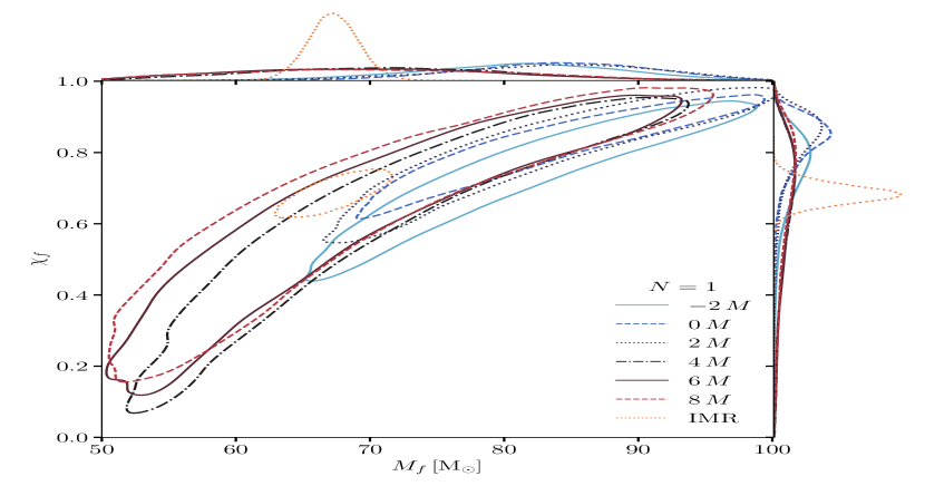
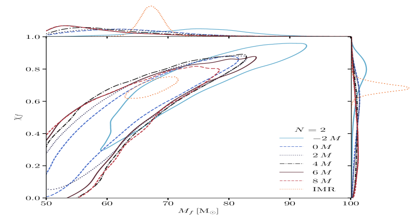
Figure 1: The posterior distributions of the final mass $M_{f}$, and the final spin $\chi_{f}$, of the GW150914 remnant were obtained utilizing the $\mathcal{F}\text{-statistic}$ method. The contours depicted in different colors correspond to different start times $\Delta t$, ranging from $-2\,M$ to $8\,M$. Results derived from fundamental-mode-only analyses are displayed on the left panel, while those incorporating the first overtone mode are presented on the right panel. Contours are shown at the $90\%$ credible level. The full IMR analysis results are indicated by dotted orange contours (Abbott et al., 2021a). Additionally, the marginal posterior distributions for both $M_{f}$ and $\chi_{f}$ are shown in their respective top and right panels.

The Bayesian inference is conducted utilizing the Bilby package (v2.1.1; Ashton et al., 2019) and the Dynesty sampler (v2.1.2; Speagle, 2020), incorporating $1000$ live points and a maximum threshold of $1000$ Markov chain steps. In alignment with Ref. (Wang and Shao, 2023), $\Delta t=t_{c}-t_{\rm ref}$ discretely spans from $-2\,M$ to $8\,M$, where the constant $M$ uses the final remnant mass of GW150914, $M=68.8\,{\rm M}_{\odot}$. Our selection of these start times is also informed by the methodologies used in other studies, such as (Cotesta et al., 2022), where similar considerations were made. The geocentric time of GW150914 is denoted by $t_{\rm ref}=1126259462.40854$ GPS while $t_{c}$ signifies the hypothesized commencement time of the ringdown signal. For the parameters $M_{f}$ and $\chi_{f}$, we use the same priors as in Ref. (Wang and Shao, 2023). The prior $\iota$ is set as $\pi(\iota)\propto\sin\iota$. The application of $\mathcal{F}\text{-statistic}$ requires flat priors for $\bm{B}$ (Prix and Krishnan, 2009), and we set the maximum of the amplitude $A_{\ell mn}$ as $5\times 10^{-20}$.

In the pursuit of evidence for the first overtone mode, we execute Bayesian inferences on two distinct models. The first model considers only the fundamental mode within the ringdown waveform, denoted as $N=1$. Our second model incorporates both the fundamental and first overtone modes, denoted as $N=2$. For each mode, we perform Bayesian inferences with different start times range from $-2M$ to $8M$. A summary of posterior distributions for the final mass ($M_{f}$) and final spin ($\chi_{f}$) can be found in Fig. 1.

In the $N=2$ model, a smaller $\Delta t$ imposes more stringent constraints on the remnant. The joint distributions exhibit bias when $\Delta t=-2\,M$, due to the inclusion of signals from nonlinear regions. Optimal constraints are achieved at $\Delta t=0\,M$, where $M_{f}=62.9^{+13.9}_{-10.4}\,{\rm M}_{\odot}$ and $\chi_{f}=0.55^{+0.25}_{-0.40}$ at a credible level of $90\%$. However, for the $N=1$ model, joint distributions scarcely encompass median values from IMR until $\Delta t$ reaches $6\,M$. This is consistent with previous studies indicating that overtone modes dominate during early stages of the ringdown signal (Giesler et al., 2019). At $\Delta t=8\,M$, remnant constraints are given by $M_{f}=70.0^{+17.2}_{-16.0}\,{\rm M}_{\odot}$ and $\chi_{f}=0.70^{+0.19}_{-0.44}$ with the $90\%$ credible level. As a comparison, using the traditional TD method, Wang and Shao (2023) reported $M_{f}=68.5^{+16.7}_{-13.9}\,{\rm M}_{\odot}$ and $\chi_{f}=0.65^{+0.24}_{-0.46}$ at the $90\%$ credible level with a Bayes factor of $-0.2$ for the $N=2$ model when $\Delta t=0M$. We find that constraints provided by the $\mathcal{F}$-statistic method are slightly tighter. Consistent with this, the $\mathcal{F}$-statistic method yields a higher Bayes factor. However, this conclusion may suffer from different priors on amplitudes and phases. We will investigate the effects of different priors for the $\mathcal{F}\text{-statistic}$ method in future work.

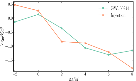
Figure 2: The logarithmic Bayes factors between models $N=2$ and $N=1$ for different $\Delta t$. For comparative purposes, we also display results from injection tests (indicated by an orange line and “$\star$” markers), which are based on a GW150914-like NR waveform.

To ascertain the presence of the first overtone mode in the GW150914 signal, we show the logarithmic Bayes factors between models $N=2$ and $N=1$ in Fig. 2. For $\Delta t=0\,M$, the logarithmic Bayes is $\log_{10}\mathcal{B}^{N=2}_{N=1}=0.1$, which does not support the model incorporating the first overtone mode. The Bayes factor decreases as $\Delta t$ increases, since the analyzed ringdown signal is shorter for larger $\Delta t$.

To conduct a more in-depth analysis, we run an injection test witn a NR waveform SXS:BBH:0305, which is similar to GW150914 and is found within the Simulating eXtreme Spacetimes catalog (Boyle et al., 2019). The waveform characterizes a source with a mass ratio of $0.82$ and a remnant with dimensionless spin $\chi_{f}=0.69$. We fix the chirp mass to $31\,{\rm M}_{\odot}$ therefore fixing the constant $M$ in this scenario to $M=68.2\,{\rm M}_{\odot}$. A luminosity distance of $490\,{\rm Mpc}$ is utilized along with an inclination angle of $3\pi/4$, while other parameters remain consistent with values established in the early study Wang and Shao (2023). The waveform corresponding to the spherical harmonics, where both azimuthal and magnetic quantum numbers are equal ($l=|m|=2$), is injected into Gaussian noise derived from GW data surrounding the GW150914 event. In this case, the post-peak signal’s SNR is approximately $14.4$ which bears similarity to that of GW150914.

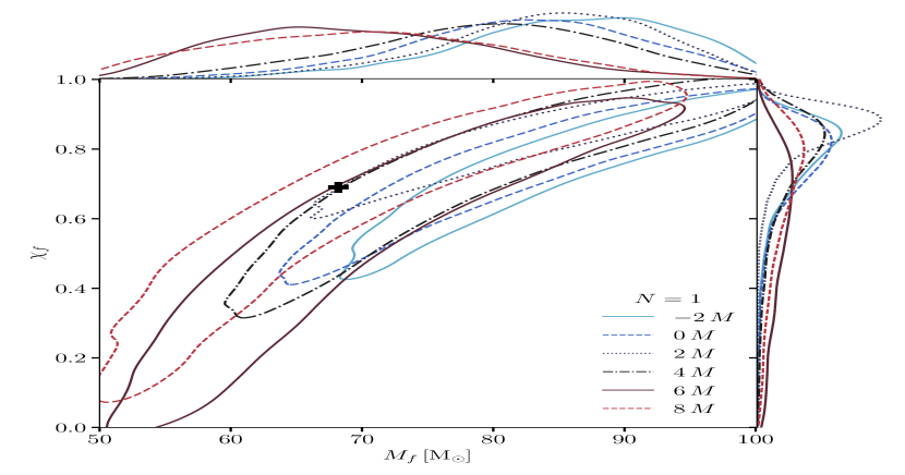
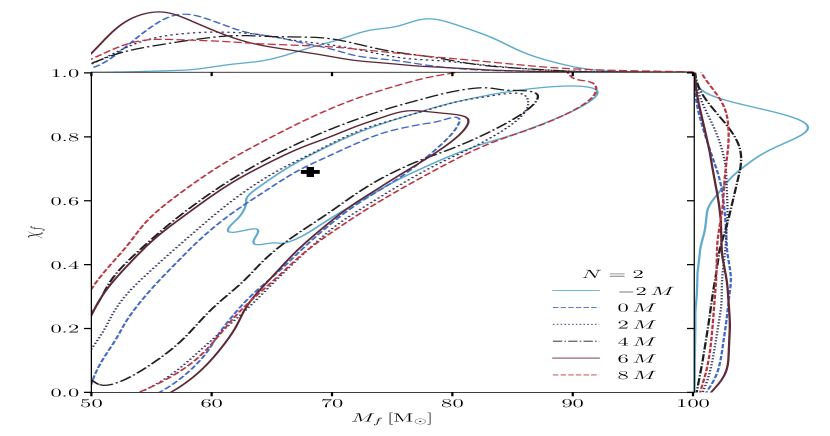
Figure 3: Similar to Fig. 1, but from the injection test. The black “+” marker represents values of the final mass $M_{f}=68.2\,{\rm M}_{\odot}$ and final spin $\chi_{f}=0.69$ in the injection.

Following the injection process, we execute TD Bayesian inferences with the $\mathcal{F}\text{-statistic}$ method for different $\Delta t$ values. The posterior distributions for both redshifted final mass $M_{f}$ and final spin $\chi_{f}$ are shown in Fig. 3. For models denoted as $N=1,2$, their joint distributions bear resemblance to those depicted in Fig. 1. The corresponding logarithmic Bayes factors are presented in Fig. 2. When $\Delta t=0\,M$, the logarithmic Bayes factor is around $0.3$. In the $N=2$ model, the final mass and final spin are $66.1^{+16.1}_{11.5}\,{\rm M}_{\odot}$ and $0.55^{+0.29}_{-0.44}$ respectively with the $90\%$ credible level. In contrast, for the case where $\Delta t=8\,M$ with $N=1$, the constraints on both final mass ($M_{f}$) and final spin ($\chi_{f}$) are $70.1^{+17.8}_{16.5}\,{\rm M}_{\odot}$ and $0.70^{+0.20}_{-0.49}$ respectively, also at a $90\%$ credible level. This suggests that incorporating the first overtone mode into the ringdown analysis could potentially enhance constraint precision slightly. Overall, there is a substantial agreement between outcomes derived from injection tests when compared with those obtained from GW150914.

IV Discussion and Conclusion

We conducted a re-analysis of the ringdown signal from GW150914 utilizing the $\mathcal{F}\text{-statistic}$ method, which possesses three primary advantages (Wang et al., 2024). Firstly, this approach ensures that the parameter space does not expand with an increased number of QNMs incorporated into the ringdown waveform. Secondly, it operates more efficiently as extrinsic parameters such as amplitudes and phases are analytically maximized over in the log-likelihood. Thirdly, this method offers flexibility for extension to other research areas, including tests of the no-hair theorem. Leveraging these benefits allows us to effectively analyze GW150914’s ringdown signal.

We scrutinize the ringdown signal of GW150914 utilizing two distinct models. The initial model encompasses solely the fundamental mode, denoted as $N=1$. The second model incorporates both the first overtone mode and the fundamental mode, represented as $N=2$. We execute Bayesian inferences for each respective model with a total of six different start times range. For the case of $\Delta t=0\,M$ when $N=2$, the final mass and spin are constrained to $M_{f}=62.9^{+13.9}_{-10.4}\,{\rm M}_{\odot}$ and $\chi_{f}=0.55^{+0.25}_{-0.40}$ respectively, at the $90\%$ credible level. Comparing the case of $\Delta t=0\,M$ with that of $N=1$, it is observed that the logarithmic Bayes factor is $\log_{10}\mathcal{B}^{N=2}_{N=1}=0.1$ which does not support the presence of the first overtone mode in GW150914. To further substantiate this conclusion, an injection test was performed. Adopting a GW150914-like NR waveform, the injection test yielded a logarithmic Bayes factor $\log_{10}\mathcal{B}^{N=2}_{N=1}=0.3$, consistent with the GW150914 case.

The findings presented here show agreement with those in Refs. (Cotesta et al., 2022; Wang and Shao, 2023; Correia et al., 2024). Specifically, compared with constraints using the traditional TD method (Wang and Shao, 2023), constraints provided by the $\mathcal{F}$-statistic method are slightly tighter. Consistent with this, the $\mathcal{F}$-statistic method yields a higher Bayes factor. However, this conclusion may suffer from different priors on amplitudes and phases. Despite this, we can anticipate the potential use of the $\mathcal{F}$-statistic method to detect subtle features within GW signals.

Undoubtedly, the analysis of the ringdown signal from additional GW events utilizing the $\mathcal{F}\text{-statistic}$ is crucial. The $\mathcal{F}\text{-statistic}$ is more efficient since extrinsic parameters can be analytically maximized. Prior to this, our intention is to incorporate the $\mathcal{F}\text{-statistic}$ into ringdown analyses for future detectors such as Einstein Telescope (Punturo et al., 2010), Cosmic Explorer (Reitze et al., 2019), Laser Interferometer Space Antenna (Amaro-Seoane et al., 2017), TianQin (Luo et al., 2016; Mei et al., 2021), Taiji (Hu and Wu, 2017), and DECIGO (Kawamura et al., 2021). Furthermore, our proposed framework exhibits flexibility for extension to BH spectroscopy based on NR waveforms and future detector-identified events. It also serves as an effective instrument for testing GR and constraining non-Kerr parameters (see e.g. Ref. Gu et al. (2024)).