Active droplets controlled by enzymatic reactions
Abstract
The formation of condensates is now considered as a major organization principle of eukaryotic cells. Several studies have recently shown that the properties of these condensates are affected by enzymatic reactions. We propose here a simple generic model to study the interplay between two enzyme populations and a two-state protein. In one state, the protein forms condensed droplets through attractive interactions, while in the other state, the proteins remain dispersed. Each enzyme catalyzes the production of one of these two protein states only when reactants are in its vicinity. A key feature of our model is the explicit representation of enzyme trajectories, capturing the fluctuations in their local concentrations. The spatially dependent growth rate of droplets naturally arises from the stochastic motion of these explicitly modeled enzymes. Using two complementary numerical methods, (1) Brownian Dynamics simulations, and (2) a hybrid method combining Cahn-Hilliard-Cook diffusion equations with Brownian Dynamics for the enzymes, we investigate how enzyme concentration and dynamics influence the evolution with time, and the steady-state number and size of droplets. Our results show that the concentration and diffusion coefficient of enzymes govern the formation and size-selection of biocondensates.
I Introduction
Recent developments of imaging techniques below the diffraction limit have shed new light on structural biology at the mesoscale. A major breakthrough came with the discovery of submicrometer membraneless compartments within cells Brangwynne et al. (2009); Banani et al. (2017), also called biocondensates. The physical mechanism behind the formation of mesoscale liquid phases in cells has gained much attention in recent years Weber and Brangwynne (2015); Zwicker (2022).
The presence of coexisting droplets in cells suggests that non-equilibrium mechanisms lead to the selection of a specific mesoscale condensate size, arresting Ostwald ripening Keber et al. (2024). Continuous descriptions relying on Flory-Huggins free energy have been designed to account for the formation of chemically active droplets Zwicker et al. (2015, 2017); Weber et al. (2019); Tjhung et al. (2018); Ziethen et al. (2023). In these models, active reactions that break detailed balance, and passive ones that respect detailed balance are allowed, with rates that are different inside and outside the droplets Zwicker (2022); Berthin et al. (2024). These models, solved at a mean-field level, predict stationary states where several droplets coexist. The role of chemical reactions in the formation of biocondensates is consistent with several experimental observations Wang et al. (2014); Guilhas et al. (2020); Linsenmeier et al. (2022); Wu et al. (2024). Specifically, post-translational modifications, namely enzyme-catalyzed reactions that change the chemical state of a protein, can modulate the strength of effective interactions between proteins, and therefore either promote or oppose the formation of biocondensates Snead and Gladfelter (2019). For instance, two enzymes catalyzing opposite reactions (phosphorylation and dephosphorylation) were correlated to the dynamics of membraneless organelles (e. g. P Granules in Caenorhabditis elegans embryos Wang et al. (2014), and postsynaptic condensates in mammalian neurons Wu et al. (2024)).
Enzymes catalyzing modifications of condensate proteins may be key controlling agents of the condensate properties Pérez et al. (2024); Smokers et al. (2024). In particular, as condensate are non-equilibrium structures, kinetics of enzymatic reactions and transport properties of enzymes should matter. In this context, several questions emerge. The concentration of each type of enzyme is governed by the genetic metabolism, the kinetics of which leads to a variety of complex dynamical patterns at the heart of systems biology Alon (2006). In the field of biocondensates, how does the enzyme concentration qualitatively and quantitatively control the structural properties of the system? Moreover, active mechanisms are known to dramatically affect the diffusion of enzymes towards or within the condensate. What is the influence of the effective diffusion coefficient of enzymes on the phase separation process at play in the formation of biocondensates?
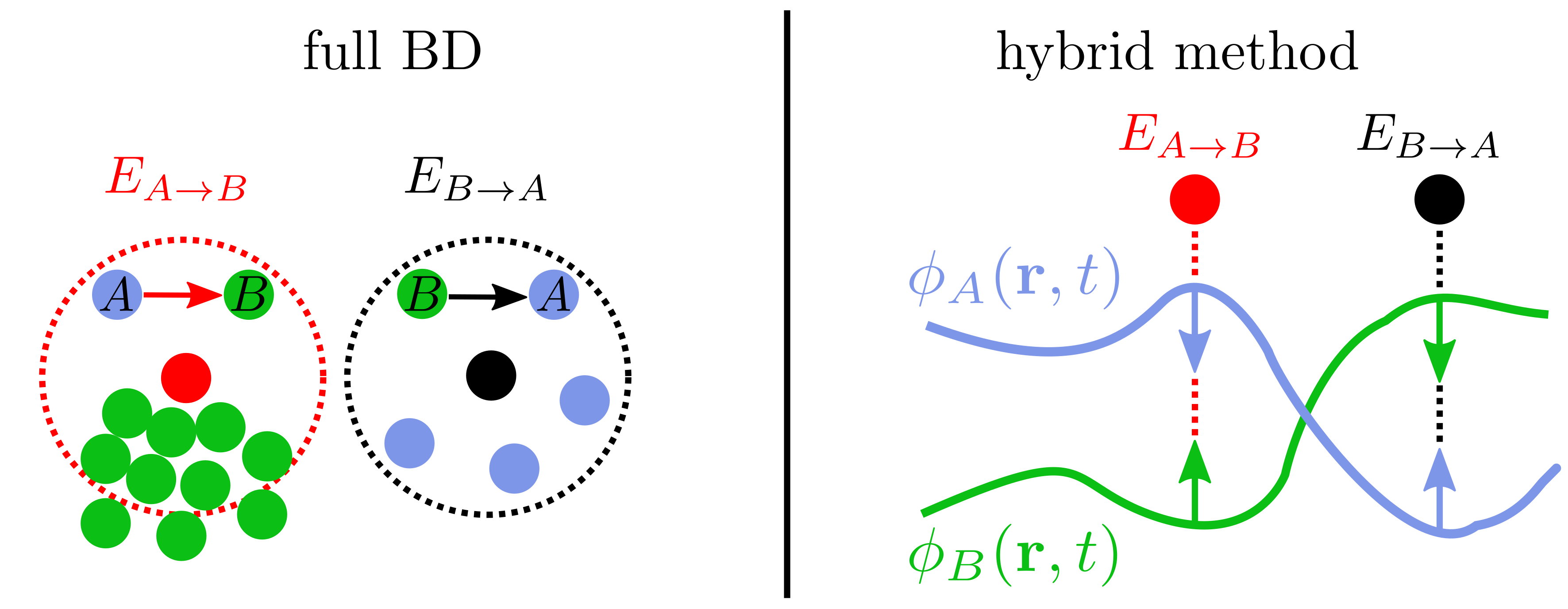
To address these questions, we propose to model the space and time evolution of biocondensates generated by attractive interactions between proteins, and modulated by chemical reactions mediated by enzymes. Models describing phase separation and chemical kinetics using Flory-Huggins theory and dynamical equations rely on an artificial density-dependent kinetic rate Weber et al. (2019); Zwicker (2022). In contrast, we adopt here a more realistic approach. Enzymes are explicitly described by discrete Brownian particles. These enzymes catalyze the switch of a protein from a condensation-prone state, favorable to droplet formation, to a dispersion-prone state. In our model, these biochemical reactions only occur when enzymes are near the two-state proteins. We consider two types of enzymes, the first one catalyzing a reaction favoring the dispersion-prone state of the protein, and the second one catalyzing the opposite reaction leading to the condensation-prone state.
We resort to two complementary numerical methods to explore the influence of enzyme concentration and dynamics on biocondensates, in 2D : (1) Reactive all-particle Brownian Dynamics simulations (these will be called ‘full BD’ in what follows), and (2) A hybrid method (HM) based on Cahn-Hilliard-Cook diffusion equations for the droplet material (the two-state protein), and Brownian Dynamics for the enzymes. Within both simulation schemes, the trajectories of enzymes are explicit. The second method allows us to check the transferability of full Brownian Dynamics results to more standard mean field models of phase transition dynamics, and to study larger system sizes. With both methods, the concentration and the diffusion coefficients of enzymes are shown to influence the number and size of condensates at steady-state. We account for the time evolution of the size of condensates in full BD with a simple analytic model.
II Models
We investigate the behavior of a binary mixture of and proteins, that undergo interconversion reactions , and where proteins attract each other and may form droplets, representing the biocondensates. The reactions and are respectively catalyzed by enzymes called and . We assume that these reactions do not take place without enzymes. These enzymes are explicitly represented, but with a highly coarse-grained representation, as disks. Note that these two reactions are coarse-grained representations of processes that involve hidden chemical reactions. Indeed, in a biological context, one of these two reactions would be coupled to a favorable secondary reaction, such as ATP hydrolysis. Moreover, as for all catalysts, an enzyme should facilitate the reactions in both ways (in our case, and ). For each one of the two reactions catalyzed by and enzymes, we consider that the reverse reaction is much less likely than the forward reaction, and is thus neglected (this assumption is justified in appendix B). We restrict ourselves to two-dimensional systems with periodic boundary conditions.
In full Brownian Dynamics, and proteins are explicitely represented. The number of enzymes is varied from one simulation to another, and these particles are replaced if necessary by non-catalyzing neutral particles to keep the total number of particles , and thus the overall surface fraction, constant. We denote by the species of particle at time . The positions of particles satisfy the overdamped Ermak (1975):
| (1) |
where is the bare diffusion coefficient of particle , and is a white noise such that and for any components or . All particles interact through a repulsive Weeks-Chandler-Andersen (WCA) potential Weeks et al. (1971), except proteins that interact through a Lennard-Jones (LJ) potential. All particles have the same diameter , which sets the length scale. Similarly, the surface densities of all the species are measured in units of All particles have the same diffusion coefficient . The WCA potential reads
| (2) |
for any couple except , where is the distance between and . We take . The Lennard-Jones potential between proteins includes an attractive part:
| (3) |
for which we set a cutoff for . The depth of the LJ potential energy well is , i.e. below the critical temperature for vapor-liquid phase equilibrium of the two-dimensional Lennard-Jones fluid Smit and Frenkel (1991), enabling proteins to form phases of contrasting densities.
Reactions are introduced in the algorithm through a random telegraph model Kampen (1976), parameterized by a reaction time . Theses reactions are only allowed in the vicinity of the enzymes Decayeux et al. (2021, 2023): when a protein of type (resp. ) is at a distance smaller than a cutoff distance from the center of the enzyme (resp. ), it becomes (resp. ) with rate (Fig. 1). Therefore, the local reaction rate is coupled to the random trajectory of the Brownian enzymes. The relationship of our model with typical biological situations is specified in appendix B, which specifies why our model is equivalent to a mixture of two enzymes respectively catalyzing a passive and an active reaction.
In the hybrid method, the positions of enzymes evolve through the overdamped Langevin equation of Brownian Dynamics, and are coupled to a binary - fluid evolving through a continuous diffusion equation Cahn (1959). The fluid is characterised by the order parameter defined as the difference in surface fraction of species and ( and cover all space , so and thus ). The free energy of the - fluid is given by a standard Ginzburg-Landau density functional Cahn (1959). The parameters are chosen so as to favor phase separation. The dynamics of the - fluid is controlled by the Cahn-Hilliard-Cook standard equation, with the addition of reactive fluxes that take place in the vicinity of each Brownian enzyme (Fig. 1).
III Arrested phase separation and emergence of non-equilibrium structures
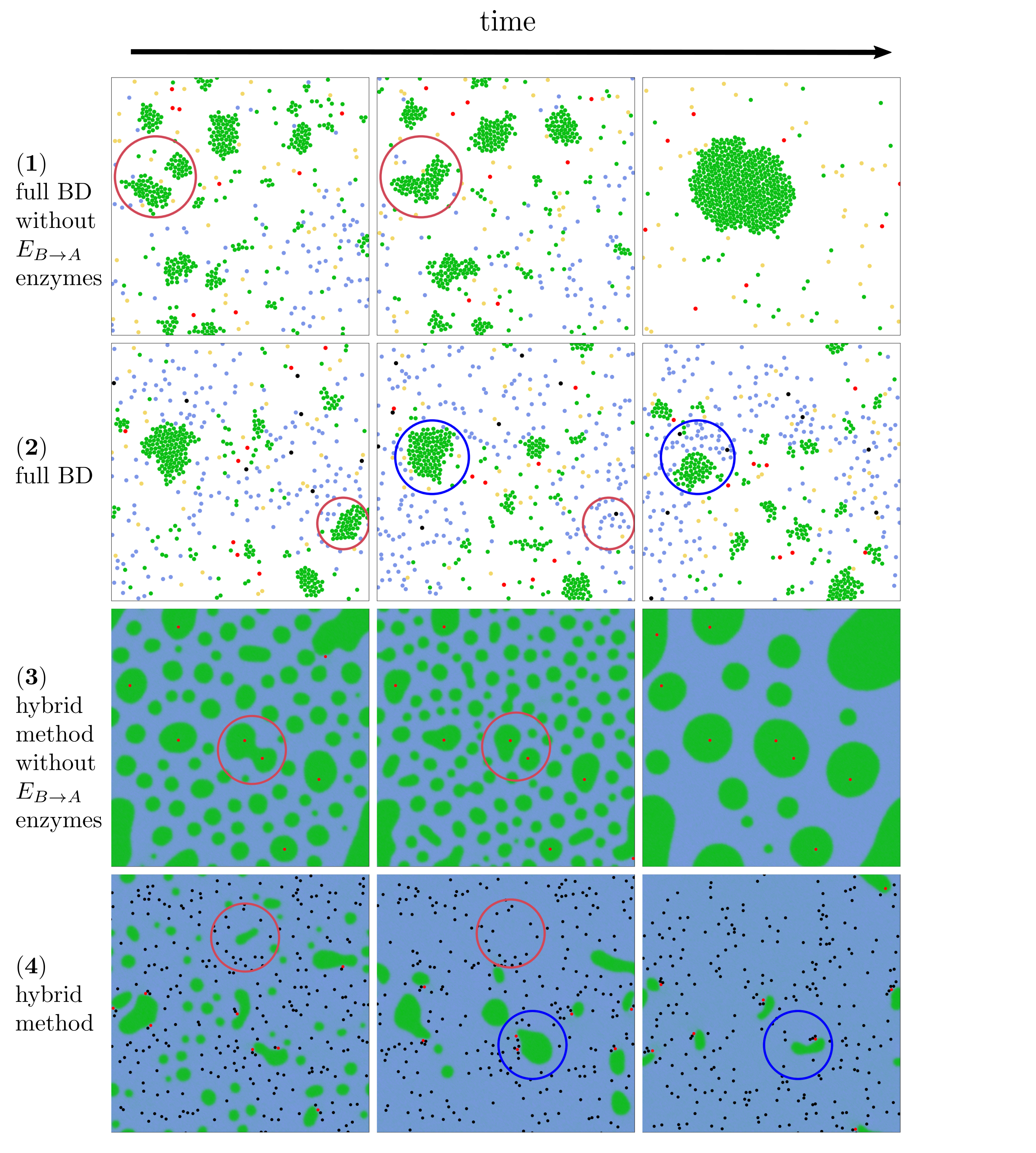
As a reference, we consider a system containing only enzymes, starting with an initial situation with only proteins in the system. In this situation, a phase separation occurs with the uninterrupted growth of droplets of proteins, as seen both in full BD and in hybrid simulations (Fig. 2-1 and 2-3). First, small droplets of proteins are formed near the enzymes, and second, the largest of these droplets of material grow at the expense of the smallest, by Ostwald ripening or by coalescence. Coalescence events are depicted in the red circles of Figs. 2-1 and 2-3. In full BD simulations, a single droplet of protein is observed at stationary state. One difference between the results of the two simulation methods is that in full BD, the enzymes continue to diffuse freely within the simulation box, even after some droplets have nucleated, whereas in the hybrid method, they remain attached to the droplets.
In the presence of both types of and enzymes, droplet growth is interrupted, as observed in both simulation schemes. Indeed, enzymes, by converting proteins into ones, either limit the growth (as depicted in the red circles of Figs. 2-2 and 2-4), or completely destroy the droplets (as depicted in the blue circles of the same figures). As we proceed to show, the balancing effect of the two types of enzymes results in the selection of a droplet size.
IV The concentration of enzymes controls the size and number of droplets
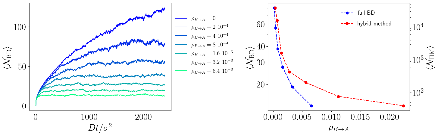
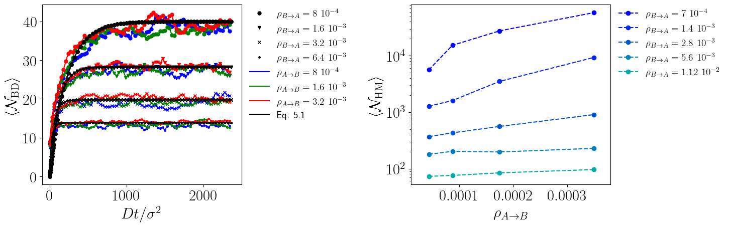
As shown in Fig. 3-left from full BD simulations, at a fixed surface concentration of enzymes, a non-zero concentration of enzymes leads to the formation of droplets that reach a finite size at stationary state. Moreover, the size of these droplets, measured by the number of proteins in a droplet , decreases as the surface concentration of enzymes increases. As previously stated, in the absence of enzymes (, blue plot), we observe the growth of a unique droplet of proteins (though the equilibrium state is not reached here, as the simulation is too short). The same general behaviour is captured by the hybrid method, as shown in Fig. 3-right, where we plot the evolution of the average size of droplets as a function of the surface concentration of enzymes, obtained from both numerical methods, on a logarithmic scale. The surface concentration of is times smaller in the HM than in full BD, leading to quantitative differences in the results. Note also that in the HM, a droplet is a cluster of contiguous cells where the concentration of dominates, and is proportional to the number of contiguous cells, as detailed in Appendix C. In contrast, a droplet in full BD is a cluster of more than proteins, as detailed in Appendix B.
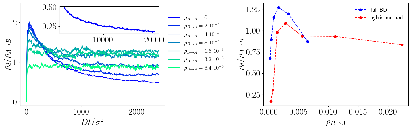
As the presence of enzymes interrupts Ostwald ripening, multiple droplets may coexist at stationary state, whose number depends on the surface concentration of enzymes, as shown in Fig. 4-left from full BD simulations at a fixed surface concentration of enzymes. In the absence of enzymes (, blue plot), we expect a ratio of at long times, as the number of enzymes is in the simulation box for this value, and a single droplet is expected at equilibrium (although the simulation time here is too short to reach this state). In all other cases, a stationary state is reached, with a mean number of droplets per enzyme larger than , indicating the formation of multiple droplets. In some cases, the number of droplets per enzyme exceeds . Interestingly, both numerical methods show a non-monotonic evolution of the number of droplets per enzyme, with a maximum appearing at roughly the same enzyme concentration (but for different values of ), as shown in Fig. 4-right. This non-monotonic behavior arises because, at low concentrations of enzymes, the number of droplets is expected to increase with from an initial value equal to at (equilibrium state). Indeed, as soon as some enzymes are introduced, the production of new proteins enables the nucleation of new droplets in the vicinity of enzymes. However, in the limit of high enzyme concentration, we expect the immediate destruction of droplets after nucleation, resulting in the disappearance of all droplets. As a result, the number of droplets passes through a maximum for an intermediate value of . There are quantitative differences between both simulation results at large values, where the decrease of the number of droplets is less pronounced with the hybrid method. With this method, B-rich droplets are always physically connected to a least one enzyme. This connection stabilizes droplets down to small sizes, even if the droplet encounters an enzyme. In full BD simulations, enzymes may diffuse away from droplets, thus making these condensates more likely to be fully destroyed under the influence of the reactions catalyzed by an enzyme.
In the range of parameters explored by full BD, it appears that the concentration of enzymes does not affect the droplet size (see Fig. 5-left), while an increase in the concentration of enzymes leads to a decrease in droplet size, as previously mentioned. This suggests that the droplets grow independently from each other around each enzyme, until they encounter an enzyme. The results from the HM, displayed in Fig. 5-right, qualitatively follow the same trend, but quantitatively differ, with the size of droplets increasing more rapidly as a function of the concentration of enzymes (note the logarithmic scale of this plot). This is likely due to the fact that the regime of enzyme concentration explored using the hybrid method differs from that examined in the full BD simulation (the concentrations of are significantly lower with the HM). This is made possible because the HM allows for the study of much larger systems than the full BD. All in all, our results show that the size of the droplets are tuned by enzyme concentrations.
V Enzyme diffusivity affects the size of condensates
When they are chemically active, the effective diffusion coefficient of enzymes can actually strongly differ from their equilibrium value, typically given by the Stokes-Einstein relation. This idea originates from the numerous sets of measurements in the biophysical literature, together with theoretical explanations which aim at relating the chemical activity of the enzyme with their diffusivity Agudo-Canalejo et al. (2018); Feng and Gilson (2020); Ghosh et al. (2021).
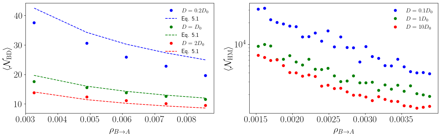
The diffusion coefficient of particles is a parameter of Brownian Dynamics simulations, and can be easily modified. Here, this value for and enzymes is either enhanced or decreased compared to the value previously used, keeping the same size for all BD particles, and the dynamic properties of all other species unchanged. As it appears in Fig. 6, the average droplet size is strongly influenced by the diffusion coefficient of enzymes: the faster are the enzymes, and the smaller are the droplets. This behavior is observed in both simulation methods. This trend may be related to the encounter time between enzymes and droplets: decreasing this time increases the effective rate of interconversion of / species.
We propose in Appendix D a simple analytic model that accounts for this behaviour. The assumptions of this model are: (i) each time a droplet encounters an enzyme, it is instantaneously destroyed, (ii) the encounter times between droplets and enzymes follow an exponential probability distribution, (iii) the encounter time between a droplet and a single enzyme only depends on the diffusion coefficients of both entities. With these assumptions, we obtain the evolution with time of the average number of particles per droplet :
| (4) |
with the surface of the simulation box, a constant that represents the influx of protein into a droplet. The encounter time is assumed to be inversely proportional to the sum of the diffusion coefficients of the droplet and of the enzyme :
| (5) |
The full BD simulation data shown in Figs. 5-left and 6-left are successfully fitted by Eq. 4, provided that we take
| (6) |
| (7) |
The dependence of with is consistent with the fact that the presence of enzymes increases the amount of proteins in the system. A higher concentration of increases the influx of proteins in the droplet. The dependence of with the size of droplets at stationary state is justified by the fact that the diffusion coefficient of the center of mass of an assembly of Brownian particles is inversely proportional to the number of particles. The agreement of this simple analytic model with full BD simulation results proves the major role played by the encounter time between a droplet and an enzyme to control the size of droplets. In the case , the comparison of simulation results with the model would work better with a slightly higher diffusion coefficient of the enzymes. Interestingly, this is consistent with calculations of the mean square displacements of the enzymes in these cases, which show a slight increase of the diffusion coefficient. We think that the interface between the two phases where the enzymes are located may push the enzymes and lead to self-propulsion. In previous studies, we have already characterize similar behaviors in a model of colloidal particle propelled by a finite size domain of Lennard-Jones particles Decayeux et al. (2021, 2023). Despite this unusual behavior, that we have to characterize in more details in future works, the ability of the model to fill all the full BD simulation data is remarkable.
The HM also shows that larger enzyme diffusivity leads to smaller droplet sizes. Despite the qualitative agreement, the analytical model does not quantitative account for the results obtained in the regime of large systems, described with the HM. From the dynamics point of view, the hybrid simulations show two singularities that explain this discrepancy with the analytical model. First, the mass transport of the / fluid does not limit the rate at which the droplet grows, as the droplet interface follows the motion of the enzymes: in all snapshots, we observe that the particles remain in contact with this interface. Secondly, a first investigation of the mean squared displacements of the enzymes suggests a strong self-propulsion in this range of parameters, which may dominate normal diffusion. Lastly, in the HM model, some enzymes are found inside droplets, which reflects the enzyme composition of real biocondensates, but that we do not account for in the simple analytical model.
VI Conclusion
In this work, we developed a simple generic model to study the interplay between two enzyme populations and a two-state protein. It is well known that biological systems regulate properties at the subcellular scale by controlling the spatial and temporal distribution of enzyme density. Enzymes selectively determine how biological components are modified and can thereby alter the physical interactions between their substrate proteins. A significant portion of enzyme-catalyzed reactions are coupled with highly exergonic processes, such as ATP hydrolysis, allowing active reactions to drive product molecules or mesoscale condensates far from equilibrium.
Here, we model a two-state protein, assumed to be the substrate of two distinct enzymes. In one state, the protein (state ) forms condensates through attractive interactions, while in the other state (state ), the proteins remain dispersed. Each enzyme catalyzes the production of one of these two protein states, promoting either protein clustering ( enzyme) or dispersion ( enzyme). Using this simple model, and employing two different simulation methods at different scales, we have demonstrated that enzyme concentration and diffusion coefficients govern the size and number of biocondensates (droplets of protein). A key feature of our model is the explicit representation of enzyme trajectories, capturing the fluctuations in their local concentrations. Unlike other models of biocondensates that rely on density-dependent reaction rates to induce size-selected droplets Zwicker (2022), our approach does not require such assumptions. The spatially dependent growth rate of droplets naturally arises from the stochastic motion of explicitly modeled enzymes.
Our minimal model suggests key design principles for enzymatic systems that regulate biocondensate properties. It opens the way to further studies integrating concepts from systems biology (networks of enzymatic reactions), macromolecule transport phenomena in biological fluids, to the dynamics of liquid-liquid phase separation at mesoscales.
Appendix A APPENDICES
Appendix B A1. Methods: All-particle Brownian Dynamics simulations (full BD)
B.1 A1a. Simulation parameters
We consider two-dimensional systems with periodic boundary conditions, that contain and proteins, and enzymes and neutral particles, also referred to as crowders. The total number of particles is fixed, ensuring the same overall density. Specifically, the number of and proteins is fixed, while the number of and enzymes varies. The total particle number is adjusted using neutral particles . All particles have the same diameter , which is used as the unit length. denotes the bare diffusion coefficient of the particles, and is used as a unit time. In all cases, the simulation box, with a length contains a surface concentration of enzymes and crowders , and a concentration of and proteins, . This corresponds to enzymes and crowders, and / proteins. The integration time step of the overdamped Langevin equation is in all cases.
The conversions of and proteins take place whenever they are within a distance to the center of an enzyme ( is taken). More precisely, at each time step, in the vicinity of an enzyme (resp. ), an protein may transform into at rate (resp. a protein may transform into at rate ). All the other reverse reactions are neglected. In all simulations, we assume that the reactions are fast compared to the diffusion characteristic time scale, and we take . The choice of the integration time step ensures that and remain much smaller than .
The characterization of the size and of the number of droplets is done using a Voronoi cell analysis. We found that the distribution of the size of Voronoi cells around proteins is bimodal, which allows us to define a threshold below which a particle can be tagged as being part of a droplet. The square root of this threshold, , is taken as the distance criteria to identify particles belonging to the same droplet. A droplet is then considered as a group composed of more than particles. From such analysis, the distribution of the number of droplets, and of the number of particles per droplet is computed, as well as moments of these distributions over time, and at stationary state. In each case, the results are averaged over independent realisations of the Brownian trajectories.
B.2 A1b. Interpreting our model : passive and active reactions in living systems
In this section, we aim at clarifying how the two kinds of chemical reactions described by our model can be considered as a couple of passive and active reactions. The term active has been used in the context of cellular metabolism for more than half a century Szent-Györgyi (1956); Jencks (1989). From a qualitative point of view, in biological systems, some reactions, referred to as active reactions, maintain the system far from equilibrium: under the influence of an active reaction , the evolution of the system composition does not relax towards chemical equilibrium (). Instead, at a specific enzymatic site, the reaction is coupled to another process associated with a negative free energy (that we shall call chemical drive Zwicker et al. (2015), noted ). This energy source may be another chemical reaction (such as ATP hydrolysis), but also the transport of particles associated with electrostatic or osmotic works Mitchell (1974). As a consequence of this coupling, the evolution of the system under the effect of the active reaction drives the system to a non-equilibrium state characterized by .
In biological systems, the same particles may be implicated in both passive and active reactions. Nevertheless, these two reactions are catalyzed by distinct enzymes. For instance, a phosphatase (a passive enzyme) catalyses the passive hydrolysis of a phosphate group bound to a protein residue, while a phosphorylase (an active enzyme) catalyzes the reverse active phosphorylation of the same protein residue, coupling this protein modification to ATP hydrolysis Shacter et al. (1984); Snead and Gladfelter (2019).
From a microscopic point of view, activity breaks the detailed balance rules that constrain the transition probabilities at play in these reactions Zwicker et al. (2015); Berthin et al. (2024). To clarify this point in the context of Brownian Dynamics simulations, we consider two configurations and of respective energies and , at two successive time steps (i.e. at times and ). These configurations only differ by the state of one particle : changes to with a probability as a result of one iteration of the forward reaction, while changes to with a probability .
When the system is at equilibrium, interconversions take place through a passive pathway. The passive conversion rates and obey the detailed balance condition:
| (8) |
where . In non-equilibrium systems, alternative active pathways may exist. In this case, the active conversion rates and break the detailed balance condition:
| (9) |
The chemical drive quantifies the deviation from equilibrium. Starting from these rules, we then explicit the specific regime corresponding to our model, with enzymes catalyzing only the forward reaction , and enzymes catalyzing only the reverse reaction.
The energies and are a combination of two terms, (1) the sum of interparticle interactions, which depends on the particle coordinates and (2) the intraparticle (or internal) free energy. We work in a regime where the difference in the internal free energies of the and species are much larger than . This quantity can be identified with the standard reaction free energy for , which has been estimated for many biological reactions and whose absolute value usually lies in the range kJ.mol-1, i.e. to Alberty (2000). This leads to several simplifications.
First, when a reaction occurs, the change in internal free energies is much larger than the contribution of interparticle interactions, which can thus be ignored. The energy difference then reads , where and are the respective internal free energies of particles and .
If the passive reaction is favored in the direction, then , , and . As we proceed to show in the next Appendix section, in such case the reactions can be neglected. In our model, this would then correspond to the rules governing the transitions of and particles in a region close to the enzyme, which could then be considered as a passive region.
Moreover, in biological systems, the active and passive pathways drive the system composition in opposite directions. In other words, the chemical drive is large enough to reverse the direction of the passive reactive flux. In the case of ATP hydrolysis as a source of chemical drive, . This quantity is in the range kJ.mol-1, i.e. about . In the case , the later conditions leads to . This implies that . The reactions can be neglected. In our model, this would then correspond to the region close to the enzyme, which could then be considered as an active region.
The symmetrical case, leads to . A reverse active reaction flux occurs for . This implies that . Under this scenario, would catalyze the active pathway, and the passive one.
All in all, our model is consistent with the coexistence of active and passive regions around two kinds of Brownian enzymes that drive the chemical composition of the system in opposite directions. The assumptions for the values of the chemical drive and for the internal free energies of the reactants and products are compatible with most real biological systems.
B.3 A1c. Influence of the presence of reverse reactions
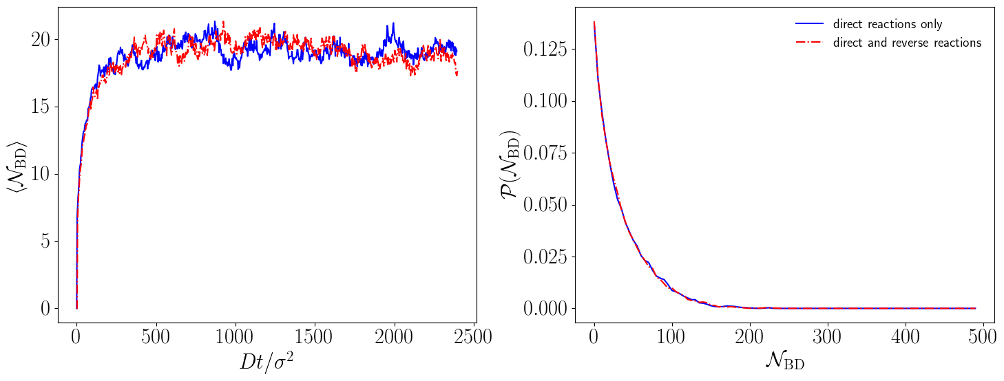
In the study described in the main text, we considered that each type of enzyme only allows a forward reaction in its vicinity ( in the vicinity of enzymes, and in the vicinity of enzymes). In order to test this assumption, we here consider a series of simulations for which the reverse reaction with a rate occurs also in the vicinity of enzyme (and respectively, the reverse reaction with a rate in the vicinity of ). Nevertheless, we keep considering systems in which the state is predominant close to enzymes and the state is predominant close to enzymes. Therefore, the rates for the reverse reactions are significantly smaller than the rates of forward reactions (, whereas ). As it is shown in Fig. 7, the time evolution of the droplet size, and the distribution of the droplet size at stationary state are unaffected by the presence of slow reverse reactions. This justifies neglecting the reverse reactions.
B.4 A1d. Influence of the range of action of the enzymes
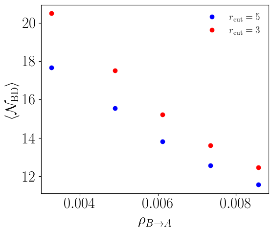
The range of action of the enzymes is controlled by the parameter . Fig. 8 presents the average size of droplets obtained with two different values of , all other parameters being unchanged, as a function of the surface concentration of enzymes. The results differ quantitatively, but they are qualitatively similar. The larger the value of , the smaller the size of the droplets at the stationary state, as their size is limited by the encounter with enzymes.
B.5 A1e. Influence of the size of the simulation box
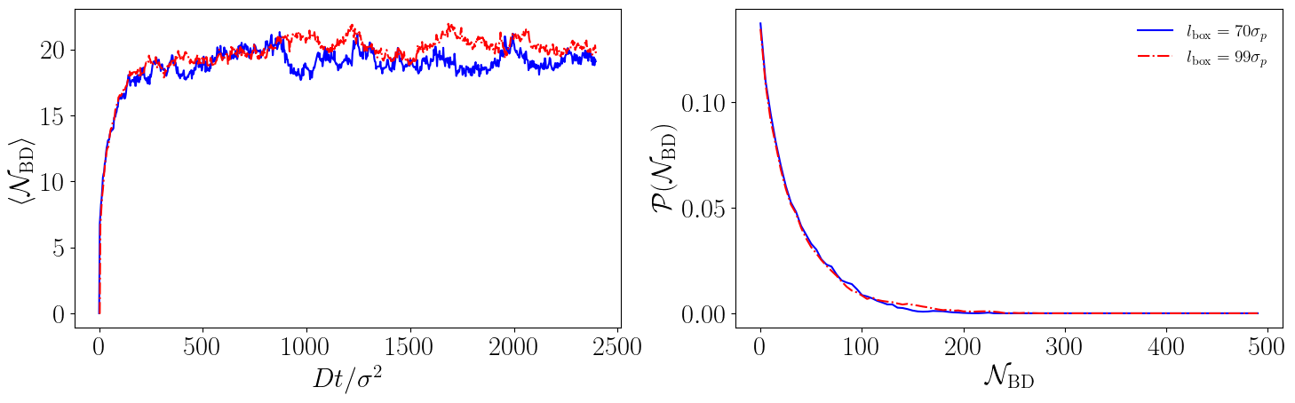
As it is shown in Fig. 9, the time evolution of the droplet size, and the distribution of the droplet size at stationary state, are not strongly affected by the size of the simulation box in full BD. In both cases, surface concentrations of particles are exactly the same, and the results are averaged over the same number of independent realisations. The same trend is found for the time evolution of the droplet size, and for the distribution of droplet size at stationary state, which shows that finite size effects in full BD simularions are negligible.
Appendix C A2. Methods: Hybrid dynamics approach (hybrid method, HM)
C.1 A2a. Model
We consider a binary mixture (BM) of two species and characterised by the order parameter , defined as the difference of surface concentration of species and . It is mixed with a suspension of enzymes, each capable of inducing either the reaction ( enzyme) or the reaction ( enzyme) in its vicinity. Each enzyme has a finite diameter , and its position is given by for .
In the absence of reactions, the total free energy of the system, called passive system, is the sum of several contributions,
| (10) |
with related to the binary mixture, to the enzyme-enzyme interaction, and to the coupling between the field and the enzyme. The free energy of the BM is given by a standard Ginzburg-Landau functional of as
| (11) |
where and specify the local free energy density, while controls the energetic penalty associated to gradients in the order parameter Cahn (1959). The minimisation of the local expression of the free energy leads to the equilibrium amplitude of the order parameter . In bulk regions far from the interfaces, where the gradients of can be neglected, we simply get . Furthermore, both linear stability analysis and minimisation of the free energy can be shown to lead to an equilibrium interface thickness (related to the largest unstable wavelength).
The enzyme-enzyme free energy contribution is a pairwise additive interaction of a completely repulsive potential that prevents overlapping
| (12) |
where is the distance between particles and . A soft repulsive Yukawa-like potential is chosen:
| (13) |
with a cutoff for distances larger than .
The particle-field interaction writes
| (14) |
where controls the strength of the particle-field interaction and controls the selectivity of the particle. The tagged function Tanaka and Araki (2000)
| (15) |
decays smoothly to zero at the corona of the enzyme for . The position of the particle will minimise the coupling free energy by segregating to regions of space where . The strength of the interaction can be quantified by the parameter with energy units .
The dynamics of the binary mixture is controlled by the Cahn-Hilliard-Cook Cahn (1959); Cahn and Hilliard (1959); Cook (1970) diffusive equation for the order parameter with the addition of a reactive flux arising from the presence of enzymes. The two coupled dynamic equations for both the field and enzyme position are
| (16a) | |||
| (16b) |
where is a mobility constant for the BM Barclay and Lukes (2019), which allows to define a diffusive time scale . A random noise is added to the Cahn-Hilliard equation, satisfying fluctuation-dissipation theorem Ball and Essery (1990). A diffusion coefficient is related to the friction and with a noise satisfying fluctuation-dissipation theorem. Two forces act on the enzyme , respectively due to the coupling with the field and the repulsive enzyme-enzyme interaction.
The flux is due to the reactions in the vicinity of enzymes. Each enzyme induces a steady conversion rate in a region of radius centered around for enzyme :
| (17) |
where is the distance between the point in space and the position of the th enzyme . The sign of depends on the type of reaction that takes place within the region: if , a enzyme transforms () into (); if , a enzyme transforms () into (). The sign of the reaction rate depends on the local average value of in the vicinity of the enzyme, such that,
| (18) |
where is the average value of within the region for a given enzyme. This means that, for an enzyme producing the protein, the reaction rate is in regions where (), while in regions where (), where no reactant is present.
C.2 A2b. Dimensionless form of the equations and parameter values
Due to the large number of parameters in eq. 16b, it is useful to express the two coupled dynamic equations in dimensionless form, as
| (19a) | |||
| (19b) |
where length are in units of , time in units of and the order parameter amplitude is scaled with . The dimensionless parameters verify:
| (20) | |||
| (21) | |||
| (22) |
The simulation box is a squared grid of points (except for Fig. 6 with a grid of points). The length scale is set such that . Then, we take for the enzyme radius , so that the size of the enzyme is comparable to the interface width between -rich droplets. The strength of the coupling with respect to enzyme thermal energy, , and with respect to the BM local energy, , are chosen to be large enough to ensure that the respective forces and chemical potential are dominant. The selectivity of both types of enzyme is , to mimic the fact that, in equilibrium () all enzymes are dispersed outside of the droplets ( species), i.e. in contact with the phase. The diffusivity of the enzyme compared to that of the BM is , to have both components diffusing in a similar time scale. The rate of reaction is , and the radius of the reaction area is The scale of the thermal fluctuations is chosen so that they are subdominant with respect to the characteristic local energy of the BM.
All simulations are initialised from a random distribution of values centered around to ensure the formation of () droplets in a matrix of (). A droplet is defined as the system region where . Standard cluster analysis are used to determine the individual droplets, to then characterise the number of droplets and the mean droplet size, defined as the average number of grid points in droplets, rescaled by the unit area . A droplet is defined as a cluster of at least grid points.
Appendix D A3. Analytic model for droplet growth
We propose a simple model to describe the evolution with time of the mean droplet size, which largely differs from the prediction of the Oswald ripening mechanism. We consider independent droplets, each made of proteins, and connected to a reservoir of proteins.
The reservoir yields a constant and equal influx of proteins towards each droplet. The droplets are assumed to be totally emptied when they encounter an enzyme, and restart growing just after the encounter. Consequently, the evolution equation for each droplet, between and is:
| (25) |
We assume now that the encounters between enzymes and droplets are memoryless, so that encounter times follow an exponential probability distribution. We call the expectation value of this distribution, corresponding to the average encounter time between a droplet and an enzyme. Therefore, the probability that the encounter takes place between and is .
Before solving this equation, we express in terms of the parameters of the model. If we neglect correlations between enzymes (low concentration regime), this characteristic encounter time can be approximated by the characteristic encounter time between a droplet and a single enzyme, divided by the number of enzymes , i.e. (with being the area of the simulation box and being the surface concentration of enzymes). Also, depends on the diffusion coefficients of both particles, and thus verifies:
| (29) |
with the diffusion coefficient of the enzyme, and the diffusion coefficient of the droplet.
Solving this differential equation with initial conditions , and using the previous expression of , yields:
| (30) |
This corresponds to Eq. 4 in the main text.
References
- Brangwynne et al. (2009) C. P. Brangwynne, C. R. Eckmann, D. S. Courson, A. Rybarska, C. Hoege, J. Gharakhani, F. Jülicher, and A. A. Hyman, Science 324, 1729 (2009).
- Banani et al. (2017) S. F. Banani, H. O. Lee, A. A. Hyman, and M. K. Rosen, Nat. Rev. Mol. Cell. Biol. 18, 285 (2017).
- Weber and Brangwynne (2015) S. Weber and C. Brangwynne, Current Biology 25, 641 (2015).
- Zwicker (2022) D. Zwicker, Curr. Opin. Colloid Interface Sci. 61, 101606 (2022).
- Keber et al. (2024) F. C. Keber, T. Nguyen, A. Mariossi, C. P. Brangwynne, and M. Wühr, Nat. Cell Biol. 26, 346 (2024).
- Zwicker et al. (2015) D. Zwicker, A. A. Hyman, and F. Jülicher, Phys. Rev. E 92, 012317 (2015).
- Zwicker et al. (2017) D. Zwicker, R. Seyboldt, C. A. Weber, A. A. Hyman, and F. Jülicher, Nature Phys. 13, 408 (2017).
- Weber et al. (2019) C. A. Weber, D. Zwicker, F. Jülicher, and C. F. Lee, Rep. Prog. Phys. 82, 064601 (2019).
- Tjhung et al. (2018) E. Tjhung, C. Nardini, and M. E. Cates, Phys. Rev. X 8, 031080 (2018).
- Ziethen et al. (2023) N. Ziethen, J. Kirschbaum, and D. Zwicker, Phys. Rev. Lett. 130, 248201 (2023).
- Berthin et al. (2024) R. Berthin, J. Fries, M. Jardat, V. Dahirel, and P. Illien, arXiv:2406.14256 (2024).
- Wang et al. (2014) J. T. Wang, J. Smith, B. C. Chen, H. Schmidt, D. Rasoloson, A. Paix, B. G. Lambrus, D. Calidas, E. Betzig, and G. Seydoux, eLife 3, 04591 (2014).
- Guilhas et al. (2020) B. Guilhas, J. C. Walter, J. Rech, G. David, N. O. Walliser, J. Palmeri, C. Mathieu-Demaziere, A. Parmeggiani, J. Y. Bouet, A. L. Gall, and M. Nollmann, Molecular Cell 79, 293 (2020).
- Linsenmeier et al. (2022) M. Linsenmeier, M. Hondele, F. Grigolato, E. Secchi, K. Weis, and P. Arosio, Nat. Commun. 13, 3030 (2022).
- Wu et al. (2024) H. Wu, X. Chen, Z. Shen, H. Li, S. Liang, Y. Lu, and M. Zhang, Molecular Cell 84, 309 (2024).
- Snead and Gladfelter (2019) W. T. Snead and A. S. Gladfelter, Molecular Cell 76, 295 (2019).
- Pérez et al. (2024) G. A. Pérez, R. V. Pappu, and D. Milovanovic, Trends in Cell Biology 34, 274 (2024).
- Smokers et al. (2024) I. B. Smokers, B. S. Visser, A. D. Slootbeek, W. T. Huck, and E. Spruijt, Acc. Chem. Res. 57, 1885 (2024).
- Alon (2006) U. Alon, An Introduction to Systems Biology: Design Principles of Biological Circuits (Chapman and Hall/CRC, 2006).
- Ermak (1975) D. L. Ermak, J. Chem. Phys. 62, 4189 (1975).
- Weeks et al. (1971) J. D. Weeks, D. Chandler, and H. C. Andersen, J. Chem. Phys. 54, 5237 (1971).
- Smit and Frenkel (1991) B. Smit and D. Frenkel, J. Chem. Phys. 94, 5663 (1991).
- Kampen (1976) N. V. Kampen, Physics Reports 24, 171 (1976).
- Decayeux et al. (2021) J. Decayeux, V. Dahirel, M. Jardat, and P. Illien, Phys. Rev. E 104, 034602 (2021).
- Decayeux et al. (2023) J. Decayeux, J. Fries, V. Dahirel, M. Jardat, and P. Illien, Soft Matter 19, 8997 (2023).
- Cahn (1959) J. W. Cahn, J. Chem. Phys. 30, 1121 (1959).
- Agudo-Canalejo et al. (2018) J. Agudo-Canalejo, T. Adeleke-Larodo, P. Illien, and R. Golestanian, Acc. Chem. Res. 51, 2365 (2018).
- Feng and Gilson (2020) M. Feng and M. K. Gilson, Annu. Rev. Biophys. 49, 87 (2020).
- Ghosh et al. (2021) S. Ghosh, A. Somasundar, and A. Sen, Annu. Rev. Condens. Matter Phys. 12, 177 (2021).
- Szent-Györgyi (1956) A. Szent-Györgyi, Science 124, 873 (1956).
- Jencks (1989) W. P. Jencks, “Utilization of binding energy and coupling rules for active transport and other coupled vectorial processes,” in Methods in Enzymology, Vol. 171 (Academic Press, 1989) pp. 145–164.
- Mitchell (1974) P. Mitchell, FEBS Letters 43, 189 (1974).
- Shacter et al. (1984) E. Shacter, P. B. Chock, and E. R. Stadtman, J. Biol. Chem. 259, 12260 (1984).
- Alberty (2000) R. A. Alberty, Biochemical Education 28, 12 (2000).
- Tanaka and Araki (2000) H. Tanaka and T. Araki, Phys. Rev. Lett. 85, 1338 (2000).
- Cahn and Hilliard (1959) J. W. Cahn and J. E. Hilliard, J. Chem. Phys. 31, 688 (1959).
- Cook (1970) H. Cook, Acta Metallurgica 18, 297 (1970).
- Barclay and Lukes (2019) P. L. Barclay and J. R. Lukes, Phys. Fluids 31, 092107 (2019).
- Ball and Essery (1990) R. C. Ball and R. L. H. Essery, J. Phys.: Condens. Matter 2, 10303 (1990).