Suppressing Si Valley Excitation and Valley-Induced Spin Dephasing for Long-Distance Shuttling

Abstract

We present a scalable protocol for suppressing errors during electron spin shuttling in silicon quantum dots. The approach maps the valley Hamiltonian to a Landau-Zener problem to model the nonadiabatic dynamics in regions of small valley splitting. An optimization refines the shuttling velocity profile over a single small segment of the shuttling path. The protocol reliably returns the valley state to the ground state at the end of the shuttle, disentangling the spin and valley degrees of freedom, after which a single virtual $z$-rotation on the spin compensates its evolution during the shuttle. The time cost and complexity of the error suppression is minimal and independent of the distance over which the spin is shuttled, and the maximum velocities imposed by valley physics are found to be orders of magnitude larger than current experimentally achievable shuttling speeds. This protocol offers a chip-scale solution for high-fidelity quantum transport in silicon spin-based quantum computing devices.

Introduction.– Efficient and coherent spin shuttling has become a promising route for scalable quantum computing in silicon-based systems [Fujita2017Coherent, Mills2019Shuttling, Yoneda2021Coherent, Jadot2021Distant, Noiri2022shuttling, Boter2022Spiderweb, Zwerver2023Shuttling, Struck2024Spin]. Silicon spin qubits benefit from long coherence times due to the weak spin-orbit coupling and the availability of isotopically purified silicon [Tyryshkin2006Coherence, Burkard2023Semiconductor]. However, the natural interaction between spin qubits is the short-range exchange coupling and experimental devices have inherently limited connectivity. As a consequence, scalability to the fault-tolerant regime relies on either introducing mediated long-range coupling via large microwave resonators [Harvey-Collard2022Resonator] or else shuttling spins throughout the device to interact with distant spins [Seidler2022Conveyor, Langrock2023Blueprint, Xue2024Si].

Initial considerations of shuttling primarily focused on the charge and spin degrees of freedom, but it is widely recognized that the valley degree of freedom inherent to silicon [Zwanenburg2013Silicon] poses a significant challenge for long-range shuttling operations. Valley splitting has been shown to vary significantly even over small distances [Lima2024Valley], and efforts to model this fluctuation have considered both deterministic and disorder-dominated regimes [Tariq2019Effects, Gamble2013Disorder, Ruskov2018Electron, Friesen2007Valley]. Experimental studies have shown coherent charge shuttling over several microns, but phase coherence has only been demonstrated in closed loops or over shorter distances where valley variability likely plays a less critical role [DeSmet2024High, Zwerver2023Shuttling, Struck2024Spin]. In a longer-distance implementation, the spin will inevitably have to be shuttled through regions where the valley splitting is small [Losert2024Strategies], leading to transitions between the instantaneous valley eigenstates. This affects the quantum information stored in the spin degree of freedom through the dependence of both the spin exchange coupling and $g$-factor on the valley state [Hwang2017Impact]. Thus, valley excitations give rise to spin-valley entanglement, which, if left unchecked, induces dephasing of the spin qubits.

Strategies for mitigating valley-induced dephasing during spin shuttling have recently gained attention, either through optimizing inter-dot tunnel couplings for a bucket-brigade approach [Feng2023Control], sharpening quantum well interfaces and/or introducing Ge doping to increase valley splitting for a conveyor-mode approach [Losert2023Practical, Losert2024Strategies], optimizing the shuttle pulses to enhance adiabaticity [Losert2024Strategies, Lima2024Superadiabatic] or detour around locations with dangerously small valley splittings [Losert2024Strategies]. These strategies require advanced capabilities and one is still left with an infidelity that grows with shuttle distance.

This paper introduces a simple shuttling protocol designed to suppress valley-related errors over a shuttle of arbitrary distance. The main idea is that, as long as the shuttle time is less than the valley relaxation time, the spin-valley entanglement produced by the shuttle is deterministic and does not constitute dephasing. Only if the valley state stochastically relaxes while entangled with the spin is the quantum information lost. Thus, one may allow nonadiabatic valley dynamics as long as one then brings the valley back into an eigenstate at the end, disentangling it from the spin and producing only a deterministic spin rotation.

In particular, we split the shuttling into two segments: one segment comprises nearly the entire length of the shuttle path, and the spin is simply moved as fast as possible in this segment, resulting in an uncontrolled but deterministic valley excitation and spin-valley entanglement. The other segment is a small region about one of the valley avoided crossings (e.g., the last one in the shuttle path, as in Fig. 1), which we refer to as a small local minimum (SLM). Around the selected SLM, we leverage intuition gained from Landau-Zener (LZ) dynamics and apply optimized control strategies to return the valley to the ground state [Ivakhnenko2023Nonadiabatic, Vitanov1996LandauZener]. The entire shuttle produces an uncontrolled but deterministic rotation of the spin about the $z$-axis of the Bloch sphere, which can easily be characterized and compensated virtually.

This approach has several attractive features. Since the optimized part of the shuttle pulse is independent of the total distance, the only limitation on distance is that the maximum shuttle speed must allow traversal within the valley relaxation time. For instance, a shuttle rate $\sim 100$ m/s and a relaxation time $\sim 1$ ms allows distances of several mm, opening up chip-scale high-fidelity shuttling. Even more enticingly in the short term, if one does not have a spatial map of the valley splitting [Volmer2024Mapping] over the entire shuttle path in order to carry out a theoretical optimization of the ramping pulse a priori, our protocol is simple enough and converges quickly enough that one can straightforwardly find the optimal shuttle pulse experimentally in situ via a gradient-free Nelder-Mead optimization.

Below, we first describe the minimal model used in our analysis which captures the relevant spin-valley coupling dynamics, followed by an introduction to the shuttling optimization protocols. Then we describe an approximation of the valley Hamiltonian that allows us to map the system to a LZ problem via a frame transformation. Using this insight, we form an ansatz and initial seed for numerical or experimental optimization. Then we demonstrate the rapid convergence of this approach. Finally, we conclude by discussing the implications of this work for quantum computing.

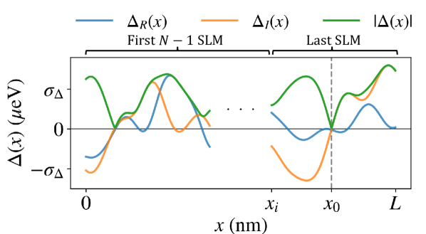
Figure 1: Schematics of real (blue), imaginary (orange) and magnitude (green) of valley landscapes as function of position. We distinguish between the first $N-1$ SLM, through which the electron is shuttled as quickly as possible, and the last SLM, located at $x_{0}$, over which the velocity profile is optimized. The parameter $\sigma_{\Delta}$, typically in the order of $100\,\mu$eV sets the magnitude of the valley splitting fluctuations.

Spin-shuttling model.– Following Ref. [Losert2024Strategies], we consider the spin-shuttling dynamics in the valley-spin coupling model described by the minimal Hamiltonian

$$\begin{split}H(x)=\frac{\omega_{B}}{2}\sigma_{z}+\frac{1}{2}\vec{\Delta}(x)\cdot\vec{\tau}\otimes\left(1+\frac{\delta\omega_{B}}{|\Delta(x)|}\sigma_{z}\right).\end{split}$$ (1)

Here, $\omega_{B}$ is the Zeeman splitting energy of the spin degree of freedom, $\vec{\Delta}=(\Delta_{R},\Delta_{I})$ where $\Delta_{R}(x)$ and $\Delta_{I}(x)$ are the real and imaginary parts of the complex-valued intervalley coupling $\Delta(x)=\Delta_{R}(x)+i\Delta_{I}(x)$, and $\delta\omega_{B}$ is the difference in Zeeman splittings for the two valley states. The Hamiltonian includes both spin and valley degrees of freedom, where $\vec{\tau}=(\tau_{x},\tau_{y})$ and $\vec{\sigma}=(\sigma_{x},\sigma_{y},\sigma_{z})$, are Pauli operators acting on the valley and spin, respectively. The variations in intervalley splitting lead to regions where transitions between valley states can occur. Due to the difference in Zeeman splittings for each valley state, this leads to spin-valley entanglement in the shuttling process, in turn causing dephasing and degraded fidelity upon stochastic collapse of the valley state.

We begin by temporarily neglecting the backaction of the spin-valley coupling on the valley evolution, thus focusing on the dynamics of the valley states alone. The spin contribution is weak compared to typical magnitudes of intervalley couplings, and as shown in the Supplementary Material (SM) [SM] exerts minimal influence on valley state evolution. Thus, the pure valley Hamiltonian as a function of position $x$ simplifies to

$$H_{\mathrm{V}}(x)=\frac{\Delta_{R}(x)}{2}\tau_{x}+\frac{\Delta_{I}(x)}{2}\tau_{y},$$ (2)

where the splitting between the valley states is $E_{v}=|\Delta|$. The main degree of freedom is the shuttling velocity $v(t)$, which enters the Hamiltonian via the standard relationship $x(t)=\int_{0}^{t}v(s)ds$, and naturally gives rise to the time-dependent valley Hamiltonian $H_{\mathrm{V}}(t)=H_{\mathrm{V}}(x(t))$ and the time-ordered propagator $U_{\mathrm{V}}(t_{2};t_{1})=\mathcal{T}_{+}e^{-i\int_{t_{1}}^{t_{2}}H_{\mathrm{V}}(s)ds}$. This approach allows us to focus on constructing a velocity profile for the electron that minimizes valley transitions while ensuring that the electron is shuttled efficiently.

Overview of shuttling optimization protocols.– The primary goal of the proposed shuttling protocol is to nonadiabatically transport the electron from position $x=0$ to $x=L$ across multiple SLMs such that it ends up in the ground valley eigenstate. After the shuttling, a $z$-rotation is implemented on the spin at the end, to undo the phase accumulated during the shuttling. The protocol starts by identifying the location of one SLM. For the sake of simplicity we will take this to be the last SLM on the path, located at a position $x=x_{0}$, although any one would work. Then, the electron is shuttled at the maximum possible speed from $x=0$ to a point $x_{i}$, chosen such that $|\Delta(x_{i})|\gg|\Delta(x_{0})|$, as shown in Fig. 1. The nonadiabatic traversal of the SLMs along the way transforms the valley state into $\ket{\psi(x_{i})}=\cos(\theta_{i}/2)\ket{0}+e^{i\phi_{i}}\sin(\theta_{i}/2)\ket{1}$ with Bloch angles $(\theta_{i},\phi_{i})$, which generally differs from an instantaneous valley eigenstate.

This allows us to treat the electron’s passage through regions of small valley splitting as a controlled LZ transition by tuning the velocity profile. Denoting $t_{i}$ such that $x(t_{i})=x_{i}$, the goal of the optimization is to find the velocity profile $v(t)$ for $t_{i}\leq t\leq t_{f}$ with the condition that $\ket{\psi(L)}=\ket{\psi_{-}}$, by which we denote the instantaneous valley ground state satisfying $H_{\mathrm{V}}(L)\ket{\psi_{-}}=-\tfrac{1}{2}|\Delta(L)|\ket{\psi_{-}}$. More concretely, we aim to maximize the state fidelity

$$\begin{split}\mathcal{F}_{\mathrm{V}}(t)&=|\bra{\psi_{-}}U_{\mathrm{V}}(t;t_{i})\ket{\psi(x_{i})}|^{2},\end{split}$$ (3)

at $t=t_{f}$, so the optimization problem is defined by

$$\begin{split}v_{\mathrm{opt}}(t)&=\operatorname*{arg\,max}_{v(t)}\mathcal{F}_{\mathrm{V}}(t_{f}).\end{split}$$ (4)

We consider two extreme cases: i) the valley landscape is completely characterized around the SLM in question, and we give a valley-informed (VI) approach; and ii) the valley landscape is completely uncharacterized, and we give a valley-agnostic (VA) approach. Obviously, there are also intermediate cases, e.g., if the magnitude of the valley splitting is mapped out but not the phase.

Valley-informed optimization.– The first step of the VI optimization protocol is to linearize Eq. (2) around $x=x_{0}$, i.e., $\Delta(x)\approx\Delta(x_{0})+\Delta^{\prime}(x_{0})(x-x_{0})$. Next, a simple unitary transformation can be used to map this linearized shuttling problem to a LZ Hamiltonian of the form $H_{\mathrm{LZ}}(x)=\alpha(x-x_{0})\tau_{z}/2+g\tau_{x}/2$. The explicit form and derivation of the LZ parameters $\alpha,g$ in terms of $\Delta(x_{0}),\Delta^{\prime}(x_{0})$ are shown in the SM [SM]. Building on intuition from LZ physics, we observe that the evolution will only induce non-trivial rotations between valley eigenstates in the region near the SLM. Thus, we define the characteristic distance $d\equiv g/\alpha$ from $x_{0}$ where $H_{\mathrm{LZ}}$ is dominated by the $\tau_{x}$ term, and the times $t_{0}$ and $\tau$ such that $x(t_{0})=x_{0}$ and $x(t_{0}\pm\tau)=x_{0}\pm d$.

In order to find an analytical expression for the action of $H_{\mathrm{LZ}}$, we approximate the total LZ evolution as a composition of three rotations, $z\rightarrow x\rightarrow z$, corresponding to the electron starting and ending far from the SLM ($|x-x_{0}|>d$), and instantaneously being shuttled to and from the SLM ($x\approx x_{0}$). We denote this approximation by piecewise evolution approximation (PEA), and the total propagator $U_{\mathrm{V}}(t_{f};t_{i})$ is then approximated by $U_{\mathrm{PEA}}=e^{-\frac{i}{2}\Theta_{3}\tau_{z}}e^{-\frac{i}{2}\Theta_{2}\tau_{x}}e^{-\frac{i}{2}\Theta_{1}\tau_{z}}$, where $\left\{\Theta_{j}\right\}_{j=1,2,3}$ correspond to the effective rotation angles in each region. This operator product has a natural interpretation as an Euler decomposition of a general unitary [McKay2017_virtual], thus enabling the treatment of the discretized evolution as a control problem under Eq. (4). By choosing $x(t)$ appropriately, and with sufficiently long shuttling times, any rotations can be achieved that takes $\ket{\psi_{i}}$ to $\ket{\psi_{-}}$.

Motivated by this scheme, we segment the shuttling process into three regions of constant velocity, namely

$$\begin{split}v(t)=\begin{cases}v_{1}&\mathrm{if}\quad|t-t_{0}|>\tau,\\ v_{2}&\mathrm{if}\quad|t-t_{0}|<\tau,\end{cases}\end{split}$$ (5)

where we imposed a symmetric condition on the velocities for simplicity. By using the PEA, the velocities $(v_{1},v_{2})$ can be found in terms of the valley parameters such that $|\bra{0}U_{\mathrm{PEA}}\ket{\psi_{i}}|^{2}=1$, where we approximate $\ket{\psi_{-}}\approx\ket{0}$ [SM]. Consequently, if one knows the valley landscape, and hence the initial state parameters $(\theta_{i},\phi_{i})$, the velocity profile obtained from the PEA is a good initial guess for a numerical gradient descent optimization of the actual valley state fidelity Eq. (3) at final time $t_{f}$. Using the ansatz of Eq. (5), we optimize only over $(v_{1},v_{2})$, while the values of $t_{0},\tau$ are obtained from the PEA.

Valley-agnostic optimization.– Even if one does not have any knowledge of the valley landscape, the exercise above suggests one should use the same piecewise constant velocity ansatz of Eq. (5) for an experimental gradient-free optimization of $v_{1}$ and $v_{2}$. However, now the location of the SLM is unknown, so $t_{0}$ and $\tau$ should also be optimization variables. Convergence is aided by choosing an initial seed pulse informed by the statistics of VI optimized pulses over an ensemble of random valley landscapes with properties that statistically reflect the device physics.

Experimentally, one applies an arbitrarily fast shuttle until reaching the selected optimization region, at which point one changes the ramping speed to the initial seed pulse drawn based on simulated VI pulses. The valley ground state probability is then measured at the endpoint and the shuttle pulse updated via the Nelder-Mead algorithm, and this whole process is to be iterated until the desired ground state fidelity is reached (otherwise the process can be restarted with a different random three-piece seed). Finally, the deterministic spin rotation along $z$ induced by the shuttle would be measured and compensated virtually via a local oscillator phase update [McKay2017_virtual].

Optimization results.– A representative example of the valley fidelity obtained from optimization can be found in Fig. 2(a) for the valley landscape near the last SLM shown in Fig. 1. Here, it can be seen that the dot spends most of the shuttling around the SLM as both VI and VA shuttle quickly to that point at speeds of $\sim 750$ and $300\,$m/s, respectively, while around the SLM dropping to within the $\pm 1\,$m/s range, reflected by the sharp change in slope in the top panel of Fig. 2(a). The intuition behind this behavior is found from the LZ problem: the electron simply needs to spend enough time near the SLM for the $\tau_{x}$ term to perform the necessary rotation.

We tested the optimization protocols on 100 different randomly generated landscapes, generated following Ref. [Losert2024Strategies], and 100 initial states given by $(\phi_{i},\theta_{i})$, for a total of $10^{4}$ test cases. For these optimizations, we consider symmetric dots of size $14\,$nm. The valley coupling is determined by the local atomic disorder in the device. Since the dot averages over the disorder, the dot size sets the length scale of valley coupling fluctuations. After determining the dot size, we chose a shuttling distance of $100\,$nm in order for at least one SLM to be present, although sometimes more than one SLM is encountered. The velocity was constrained to $<10^{3}\,$m/s to avoid orbital excitations (see Ref. [Langrock2023Blueprint]); however, that constraint was mostly irrelevant as the shuttling duration is largely dominated by waiting about the SLMs. The time evolution given by the operator $U_{\mathrm{V}}$ was implemented in Qutip [Johansson2013_qutip]. More details regarding the generation of landscapes and choice of optimization parameters can be found in the SM [SM].

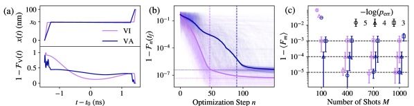
Figure 2: (a) Example of the valley landscape and optimized fidelity, for an initial state with angles $(\phi_{i},\theta_{i})=(\pi/4,\pi/2)$, over a distance of $100$ nm at an average speed of $\sim$35 m/s. Optimized electron shuttling (top) and infidelities (bottom) as functions of time, for VI and VA optimizations. (b) Median state infidelity [Eq. (3)] at final shuttling time (solid lines) as function of optimization step, for VI (purple) and VA (dark-blue) methods, up to 150 iterations. First interquartile ranges are shown as error bars but are not visible. In addition, 500 individual optimizations are shown in the background. Vertical dashed lines represent median values of total number of iteration steps. Horizontal dotted lines mark final achieved median infidelities. (c) Median noisy infidelities [Eq. (6)], averaged over 300 different combinations of landscapes and angles. Error bars are given by first interquartile ranges. Measurement error per shot of $p_{\mathrm{err}}\in\{10^{-5},10^{-4},10^{-3}\}$. Horizontal dashed lines represent the boundary set by measurement noise, where the infidelity is equal to $p_{\mathrm{err}}$. The number of shots $M\in\{100,400,700,1000\}$ have been shifted slightly for clarity.

Figure 2(b) shows the infidelity vs number of optimization iterations for both methods. Over the set of $10^{4}$ different cases, for the VI (VA) optimizations, we find a median valley state infidelity $1-\mathcal{F}_{\mathrm{V}}(t_{f})$ of $4\times 10^{-8}(4\times 10^{-7})$. The median number of iterations it took the optimizer to find solutions with a tolerance of $1-\mathcal{F}_{\mathrm{V}}(t_{f})<10^{-6}$ was 47 (90) for the VI (VA) case. Thus, one can reliably find solutions to arbitrary accuracy without any knowledge of the valley landscape with only about a factor of two more iterations than if one has the full valley map.

When the optimization is experimentally performed on hardware, the measured valley state estimated quantities will inevitably suffer from different sources of noise. To test the efficacy of the optimization when measurement noise is included, we incorporate stochastic contributions to the objective function. We model shot noise by randomly sampling state projections $q_{i}\in\{0,1\}$ with probabilities given by $\{\mathcal{F}_{\mathrm{V}}(t_{f}),1-\mathcal{F}_{\mathrm{V}}(t_{f})\}$, respectively. Then, we define the finite sampling fidelity $\overline{f}_{M}=1-\frac{1}{M}\sum_{i=1}^{M}q_{i}$, where $M$ is the number of shots, which approximates the noiseless fidelity $\mathcal{F}_{\mathrm{V}}(t_{f})=\overline{f}_{M}+O(1/\sqrt{M})$. The influence of shot noise will be more significant for superposition states, whereas for computational basis states it will be insignificant. Thus, shot noise is expected to only affect noticeably the initial part of the optimization.

We also allow for measurement noise by assuming that the wrong state $q_{i}$ was detected with uniform probability $p_{\mathrm{err}}$, so that the noisy measured fidelity is

$$\begin{split}F_{m}\left(\overline{f}_{M}\right)=\overline{f}_{M}\times\left(1-\frac{m}{M}\right)+\left(1-\overline{f}_{M}\right)\times\frac{m}{M},\end{split}$$ (6)

where $m$ is a random integer drawn from a Poisson distribution [Wasserman2004] with mean $p_{\mathrm{err}}\times M$. As opposed to shot noise, measurement noise will contribute significantly only at the end of the optimization, where the average fidelity becomes $\langle F_{m}(1)\rangle=1-p_{\mathrm{err}}$, while for equal superposition states Eq. (6) has a fixed point, namely, $\langle F_{m}(1/2)\rangle=1/2$. A different random $m$ is drawn for each call of $F_{m}$.

Optimizing with the noisy measured fidelity Eq. (6) as the objective function using Nelder-Mead for both VI and VA we obtain the infidelities shown in Fig. 2(c). Each combination of $(p_{\mathrm{error}},M)$ is optimized over a subset of 300 landscapes and initial angles, randomly sampled from the $10^{4}$ ones used previously in Fig. 2(b). The optimizer is able to approach the ground state when using more than 100 shots, saturating around the bound set by measurement error $1-\braket{F_{m}}\gtrsim p_{\mathrm{err}}$. Using the noisy objective function did not require more iterations; the average number of iterations was 47 (69) for the VI (VA) optimizations (less than the noiseless case, but only because the infidelity saturates at a higher level). Lastly, note that with $\sim 100$ shots at a single-shot measurement time under $1\,$ms [Elzerman2004] and $\sim 100$ iteration steps, we expect the optimization process to take around $10\,$s. Since near-optimal results can be quickly achieved even with noisy measurements and a gradient-free optimization method, this analysis provides optimism regarding the applicability of this method on hardware.

Conclusions.– The protocol we have proposed in this work achieves efficient suppression of valley-induced spin dephasing by leveraging intuition obtained from the LZ transition. When detailed information of the valley landscape is accessible, we perform a two-step VI optimization process to minimize valley transitions: first by mapping the linearized valley Hamiltonian to a LZ problem and solving it using the PEA; then, by refining the velocity profile through gradient descent optimization in the original valley frame. When the landscape is not known, the VA optimization uses the same ansatz motivated by the VI case, but with randomized initial conditions.

Although in this work we chose to optimize passage through the last SLM on the shuttle path for simplicity, an analogous approach can be easily formulated for any intermediate SLM instead. In the VI case this is simple because the location is known, and the evolution after the selected SLM can be computed explicitly. The solution is then equivalent to the PEA derived in this work, but targeting instead of the ground state a state that compensates for the nonadiabatic valley evolution up to that point and precompensates for the remainder following that point. The VA case introduces the additional challenge of not knowing with certainty if the optimization is being performed over just one or even no SLM. This challenge can be readily addressed, however, by including the shuttled distance as a new optimization variable, without increasing the complexity of the optimization problem substantially.

In practice, charge noise may change the shuttle path and consequently the valley landscape seen by the electron. In particular, $1/f$-type noise has been observed at kHz-MHz frequencies [Connors2022, ye2024characterizationindividualchargefluctuators, Yoneda2023, Jock2022], but with a much lower amplitude that only perturbs the dot position by $\lesssim 10\,$pm [Yoneda2017], which is much smaller than typical dot sizes and should have a negligible effect on both the VA and VI approach.

Thus, by adjusting the shuttling velocities in a simple way over a small segment of the path, a rapid, long-distance shuttle over regions of small valley splitting can achieve suppression of valley-induced dephasing independent of the shuttle distance. This protocol paves the way for chip-scale coherent transport in silicon-based quantum processors. Future work may explore further extensions of the model by incorporating other sources of dephasing, such as spin-orbit coupling and charge noises.

Supplemental Material

Appendix A Landau-Zener Instantaneous Eigenstates

The standard Landau-Zener Hamiltonian in position space is defined by

$$\begin{split}H_{\mathrm{LZ}}(x)=\frac{1}{2}\begin{pmatrix}\alpha x&g\\ g&-\alpha x\end{pmatrix},\end{split}$$ (7)

where $\alpha,g$ are assumed positive. This Hamiltonian can be diagonalized to find the instantaneous eigenstates. The eigenvalues are $E_{\pm}=\pm\frac{1}{2}\sqrt{g^{2}+\alpha^{2}x^{2}}$. In the same basis as $H_{\mathrm{LZ}}$ in Eq. (7), the unnormalized eigenstates become

$$\begin{split}\ket{\psi_{\pm}(x)}\dot{=}\begin{pmatrix}g\\ \alpha x\pm\sqrt{\alpha^{2}x^{2}+g^{2}}\end{pmatrix},\end{split}$$ (8)

with $\ket{\psi_{-}}$ denoting the ground state with energy $E_{-}$. At a distance $D$ away from the avoided crossing, for $g\ll\alpha D$, the eigenstate can be expanded to obtain

$$\begin{split}\ket{\psi_{-}(D)}\approx\ket{0}-\frac{g}{2\alpha D}\ket{1}.\end{split}$$ (9)

Thus, we may write $\ket{\psi_{-}(D)}=\ket{0}+O(g/\alpha D)$.

Appendix B LZ Evolution

The first step of the VI optimization protocol is to linearize the intervalley coupling near the SLM located at $x_{0}$, namely

$$\begin{split}H_{\mathrm{V}}^{\mathrm{lin}}(x)=\left(\left.\vec{\Delta}(x_{0})+\frac{d\vec{\Delta}}{dx}\right|_{x_{0}}(x-x_{0})\right)\cdot\frac{\vec{\tau}}{2},\end{split}$$ (10)

where $x_{0}$ is defined such that $\left[\frac{d}{dx}|\Delta(x)|\right]_{x_{0}}=0$, from which the simple relationship between the phases of the coupling and its derivative can be derived, i.e., $\arg\Delta^{\prime}(x_{0})=\arg\Delta(x_{0})+\pi/2$. Next, to relate the linearized problem with a LZ transition, we define the unitary transformation

$$\begin{split}U_{R}=R_{y}(-\pi/2)R_{x}(\pi/2)R_{z}\left(\arg\Delta(x_{0})\right),\end{split}$$ (11)

where $R_{k}(\phi)=e^{-\frac{i}{2}\phi\tau_{k}}$. Here, the initial $z$-rotation combines the position-dependencies of the two terms, followed by $x-$ and $y-$rotations to relabel the axes to match the standard LZ form. Implementing this rotation onto $H_{\mathrm{V}}^{\mathrm{lin}}(x)$, it simplifies to the traditional LZ Hamiltonian

$$\begin{split}H_{\mathrm{LZ}}(x)&=U_{R}H_{\mathrm{V}}^{\mathrm{lin}}(x)U_{R}^{\dagger}\\ &=\frac{\alpha}{2}(x-x_{0})\tau_{z}+\frac{g}{2}\tau_{x},\end{split}$$ (12)

where we defined the overall energy gap rate in space at the SLM as $\alpha=\left|\Delta^{\prime}(x_{0})\right|$ and the coupling magnitude as $g=|\Delta(x_{0})|$, where the relationship between the phases of the coupling and its derivative was used explicitly. An additional $R_{z}(\pi)$ rotation may be necessary to ensure $g>0$.

Furthermore, from Eq. (12) we define the characteristic distance $d\equiv g/\alpha$. Note that, since $H_{\mathrm{LZ}}(x)$ is approximately proportional to $\tau_{z}$ for $|x-x_{0}|\gg d$, the non-trivial contribution to the valley evolution will occur in the region near the SLM. As will be shown below, this allows us to treat the electron’s passage through regions of small valley splitting as a controlled LZ transition by tuning the velocity profile. Next, we analytically solve $H_{\mathrm{V}}^{\mathrm{lin}}(x)$ to obtain a good seed pulse from which to numerically optimize the actual evolution due to $H_{\mathrm{V}}(x)$.

We approximate the total LZ evolution as a composition of three rotations, $z\rightarrow x\rightarrow z$, corresponding to the electron starting far from the SLM ($|x_{0}-x|\gg d$) where the $\tau_{z}$ term dominates, then instantaneously being shuttled to the SLM ($x\approx x_{0}$) where the $\tau_{x}$ term dominates, and finally instantaneously moving far away again ($|x-x_{0}|\gg d$). We will refer to this as the piecewise evolution approximation (PEA), where the corresponding Hamiltonian that generates this evolution is

$$\begin{split}H_{\mathrm{PEA}}(x)=\frac{1}{2}\begin{cases}\alpha\,(x-x_{0})\,\tau_{z}&\mathrm{if}\quad|x-x_{0}|>d,\\ g\,\tau_{x}&\mathrm{if}\quad|x-x_{0}|<d\end{cases}.\end{split}$$ (13)

The total propagator $U_{\mathrm{V}}(t_{f};t_{i})$ is then approximated by

$$U_{\mathrm{PEA}}=e^{-\frac{i}{2}\Theta_{3}\tau_{z}}e^{-\frac{i}{2}\Theta_{2}\tau_{x}}e^{-\frac{i}{2}\Theta_{1}\tau_{z}},$$ (14)

where $\left\{\Theta_{j}\right\}_{j=1,2,3}$ correspond to the effective rotation angles in each region, written in terms of LZ Hamiltonian parameters as

$$\begin{split}\Theta_{1}&=\alpha\left[\int_{t_{i}}^{t_{0}-\tau}x(t)dt+x_{0}(t_{i}-t_{0}+\tau)\right],\\ \Theta_{2}&=g\int_{t_{0}-\tau}^{t_{0}+\tau}dt=2g\tau,\\ \Theta_{3}&=\alpha\left[\int_{t_{0}+\tau}^{t_{f}}x(t)dt-x_{0}(t_{f}-t_{0}-\tau)\right].\end{split}$$ (15)

Here we defined the times $t_{0}$ and $\tau$ such that $x(t_{0})=x_{0}$ and $x(t_{0}\pm\tau)=x_{0}\pm d$. By choosing $x(t)$ appropriately and with sufficiently long shuttling times, any rotations can be achieved. Lastly, $U_{\mathrm{PEA}}$ can be interpreted as an Euler decomposition of a general unitary [McKay2017_virtual], thus enabling the treatment of the PEA evolution as a control problem. An example of this evolution is shown in Fig. 3.

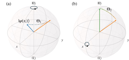
Figure 3: Composition of rotations in the PEA, with blue vector corresponding to the initial state $\ket{\psi(x_{i})}$ in the LZ frame. (a) $z$-rotation bringing the initial state $\ket{\psi(x_{i})}$ to the $yz$-plane, where the orange vector corresponds to the state $R_{z}\left(\Theta_{1}\right)\ket{\psi(x_{i})}$. (b) $x$-rotation bringing the intermediate state to the $\ket{0}$ state, where the green vector corresponds to the state $R_{x}\left(\Theta_{2}\right)R_{z}\left(\Theta_{1}\right)\ket{\psi(x_{i})}$.

As the electron moves away from the SLM, the instantaneous ground state $\ket{0}$ approaches the valley ground state, $\ket{0}=\ket{\psi_{-}}+\mathcal{O}(d/D)$ [SM]. Since in cases of interest $D\gg d$, we use $\ket{0}$ as the PEA target state. To find the transformation of interest, we first parameterize the initial valley state at the starting location $x_{i}$ in standard Bloch sphere representation [Nielsen2012],

$$\ket{\psi(x_{i})}=\cos(\theta_{i}/2)\ket{0}+e^{i\phi_{i}}\sin(\theta_{i}/2)\ket{1}.$$ (16)

Then, we find the Bloch angles $(\phi,\theta)$ in the LZ frame by computing $U_{R}\ket{\psi(x_{i})}=\cos(\theta/2)\ket{0}+e^{i\phi}\sin(\theta/2)\ket{1}$. From Eq. (14), $U_{\mathrm{PEA}}\ket{\psi(x_{i})}=\ket{0}$ if

$$\begin{split}\Theta_{1}&=\frac{\pi}{2}-\phi+2\pi n_{1},\\ \Theta_{2}&=\theta+2\pi n_{2},\end{split}$$ (17)

where the choice of integer $n_{1}(n_{2})$ correspond to the number of complete circuits rotated about the $z(x)-$axis. The choice of $\Theta_{3}$ is arbitrary.

Next, we find the required physical parameters in the LZ frame from these rotation angles and Eqs. (15). Following the scheme suggested by the PEA in Eq. (13), we segment the shuttling process into three regions of constant velocity, namely

$$\begin{split}v(t)=\begin{cases}v_{1}&\mathrm{if}\quad|t-t_{0}|>\tau,\\ v_{2}&\mathrm{if}\quad|t-t_{0}|<\tau,\end{cases}\end{split}$$ (18)

where we imposed a symmetric condition on the velocities for simplicity. Here, we denote $(t_{0}-\tau,t_{0}+\tau)$ the range of times over which the electron is expected to be near the SLM. Denoting $T=t_{0}-t_{i}=(D-d)/v_{1}+\tau$, integrating the first line of Eq. (15) then results in

$$\begin{split}\Theta_{1}&=\alpha\left[\frac{v_{1}}{2}(T-\tau)^{2}-D(T-\tau)\right].\end{split}$$ (19)

Noting that $\tau=d/v_{2}=g/(\alpha v_{2})$ and combining with Eq. (17) yields $\tau=\frac{\theta+2\pi n_{2}}{2g}$ and the corresponding shuttling velocities in the PEA are

$$\begin{split}v_{1}&=\frac{\alpha\left(D^{2}-d^{2}\right)}{2\phi-\pi(4n_{1}+1)},\\ v_{2}&=\frac{2g^{2}}{\alpha(\theta+2\pi n_{2})}.\end{split}$$ (20)

Lastly, the value of $t_{f}$ is set by imposing $x(t_{f})=L$, namely $t_{f}=t_{0}+\tau+(L-x_{0}-d)/v_{1}$. See next section for details on optimal choices of $n_{1},n_{2}$.

Appendix C Optimal Choices of $n_{1},n_{2},T$

As shown in Eq. (20), there exist multiple combinations of $n_{1},n_{2}$ that meet the conditions required to shuttle the electron while suppressing valley-induced dephasing. Here we propose a criterion to choose $n_{1},n_{2}$ based on efficiency under physical constraints.

First, a relationship can be derived for $n_{2}$ by enforcing $\tau>0$ and requiring $\tau$ to minimize the shuttling time under the maximum shuttling velocity constraint $|v(t)|\lesssim v_{\mathrm{max}}$. From imposing this condition on $v_{2}^{\mathrm{PEA}}$, we obtain

$$\begin{split}n_{2}^{\mathrm{opt}}=\left\lceil\frac{1}{2\pi}\left(\frac{2g^{2}}{\alpha v_{\mathrm{max}}}-\theta\right)\right\rceil,\end{split}$$ (21)

from where the minimum $\tau_{\mathrm{min}}=(\theta+2\pi n_{2}^{\mathrm{opt}})/g$ can be found. In practice, since $v_{\mathrm{max}}=10^{3}\,$m/s and $g\ll\alpha D$, this implies that $n_{2}$ is set to small values, namely 0 or $-1$.

Next, to ensure that the maximum velocity condition is met, we impose $T_{\mathrm{min}}\gtrsim\tau_{\mathrm{min}}+(D-d)/v_{\mathrm{max}}$. During the optimization, the optimizer may fail to achieve sufficiently high fidelities. When this is the case, we iterate over $T$ in the range $(T_{\mathrm{min}},2T_{\mathrm{min}})$ and find new PEA parameters. See main text for details of this performance for iterations over $T$.

Lastly, for the PEA to approximate the physical valley problem, the traversed distance near the avoided crossing $2v_{2}\tau$ must be close to the transition distance $2d$. Defining the LZ energy a distance $D$ away from the avoided crossing $\Delta_{i}=\alpha D$, we write $d$ in terms of the physical and optimal parameters,

$$\begin{split}v_{2}\tau&=D-v_{1}(T-\tau)\\ &=\frac{1}{\alpha}\left(\Delta_{i}-\left[\frac{\pi(4n_{1}+1)-2\phi}{(T-\tau)^{2}}+\frac{2\Delta_{i}}{T-\tau}\right](T-\tau)\right)\\ &=\frac{1}{\alpha}\left(-\Delta_{i}+\frac{2\phi-(4n_{1}+1)\pi}{T-\tau}\right)\end{split}$$ (22)

which, from requiring $v_{2}\tau\approx g/\alpha$, implies $(4n_{1}+1)\pi=2\phi-(T-\tau)(g+\Delta_{i})$. Consequently, we obtain

$$n_{1}^{\mathrm{opt}}=\left\lceil\frac{2\phi-\pi-(T-\tau)(g+\Delta_{i})}{4\pi}\right\rceil.$$ (23)

Thus, taking these values of $n_{1},n_{2},T$ we ensure that the PEA solution is achieved while approximating the real evolution, and at the same time imposing the physical constraint of maximum shuttling speed but maintaining shuttling efficiency.

Appendix D Optimization Details

In this section we provide the details used in the numerical optimizations performed in the main text.

For the generation of valley landscapes, we followed the steps outlined in Ref. [Losert2024Strategies] , where the authors introduced a simple way of generating realistic landscapes using a Gaussian covariance model and the Python package GSTools to generate fluctuating Si concentrations. Here, we define a symmetric dot size of $a_{x}=a_{y}=14\,$nm, which sets the correlation lengths of $\Delta_{R}$ and $\Delta_{I}$. From this dot size, we chose a shuttling distance of $100\,$nm in order for at least one SLM to be present. The covariance $\sigma_{\Delta}^{2}$ of the coupling $\Delta$ was set to $\sigma_{\Delta}=100\,\mu$eV, to match order of magnitudes observed in experimental measurements. From here, it can be derived that the covariances of $\Delta_{R}$ and $\Delta_{I}$ are given by $\sigma_{\Delta}^{2}/2$. The average valley splitting used to generate these landscapes is $\sqrt{\pi}/2\sigma_{\Delta}$. We assume the dot is the ground state of an isotropic harmonic oscillator potential with mass $m_{t}$ and level spacing $\hbar\omega=2\,$meV, giving rise to dot radii $a_{x}=a_{y}=\sqrt{\hbar/(m_{t}\omega)}=14\,$nm. Representative examples are shown in Fig. 4. Notice that some landscapes can be interpreted as presenting more than one SLM in this range, which, as explained in the main text, does not constitute a problem for our method. When multiple SLM are present, the optimization is performed over the one presenting the minimum $|\Delta(x)|$.

The 100 initial angles $(\phi_{V},\theta_{V})$ were chosen uniformly from the Bloch sphere using the Fibonacci lattice method [Swinbank2006, Gonzlez2009]. The north and south poles of the sphere, corresponding to the computational basis states, were included.

VA optimization initial seeds were drawn from normal distributions based on the mean and standard deviations of the parameters obtained from the VI optimization results. The mean and standard deviation values found from the $10^{4}$ VI optimization are: $v_{1}\in(300\pm 100)\,\mathrm{m/s},\,v_{2}\in(0.1\pm 2)\,\mathrm{m/s},\,\tau\in(1.5\pm 2)\,\mathrm{ns}$. The VA seeds were drawn using the Python package NumPy’s random.normal functionality, with center and scale parameters set to the mean and standard deviations obtained from VI, respectively. Note that if a given value of $\tau<0$ is drawn, a new value is sampled until $\tau>0$ is obtained. Lastly, the parameter $t_{0}$ is chosen to locate the middle region in the center of the shuttle, i.e., $t_{0}=\tau+(L/2-v_{2}\tau)/v_{1}$.

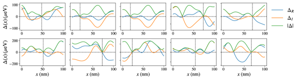
Figure 4: Representative examples of randomly generated valley landscapes used in the main text to test the optimization protocols. The landscapes were generated following the steps outlined in Ref. [Losert2024Strategies]. Vertical lines show the location of chosen SLMs around which the velocity profiles are optimized for each landscape.

Appendix E Optimization Success Rate

In this section we study the success rate of the optimizations for given initial conditions. We define the success rate in optimization as the fraction of optimizations that achieve an infidelity below $10^{-4}$. This threshold is chosen to be representative of state-of-the-art gate infidelities. The protocol employed involves first optimizing the entire set of $10^{4}$ different test cases, and then selectively reoptimizing only the cases that fail to meet the specified fidelity threshold. For VI, the attempts refer to extending the first shuttling time by increasing $T$ in the range $(T_{\mathrm{min}},2T_{\mathrm{min}})$ in steps of $0.1T_{\mathrm{min}}$. In the VA case, new initial conditions are drawn with each attempt. See Sec. C for details on the choice of $T_{\mathrm{min}}$ and the initial condition sampling of VA.

Figure 5 shows the success rates after each iteration for both methods. As shown, the VI method obtains a success rate of 88% after the first iteration, quickly achieving 99%. The VA method on the other hand, is successful on 40% of the test cases, while increasing to 90% after 10 iterations. this highlights the fact that knowledge of the valley landscape provided by the PEA initial seed in the VI case greatly improves the optimization performance. However, this also provides further support to detailed valley landscape information not being essential for the success of the optimization.

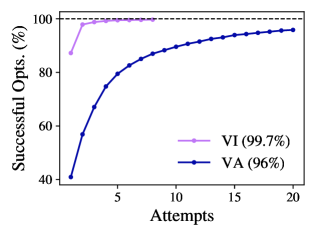
Figure 5: Comparison of optimization success rates between VI and VA. VI achieves a 99% success rate after 3 attempts, while VA reaches 90% after 10 attempts. In the plot legend we present the maximum success rates obtained after the number of attempts shown.

Appendix F Spin-Valley Backaction

Here, we analyze numerically the effect of the spin degree of freedom on the valley dynamics. We numerically simulate the spin-valley Hamiltonian Eq. (1), by choosing the velocity profile optimized shown in Fig. 2 of the main text. We calculate the ground state probability as a function of time after tracing out the spin,

$$\begin{split}\mathcal{F}(t)=\bra{0}\mathrm{Tr}_{S}\left(U(t)\rho_{i}U(t)^{\dagger}\right)\ket{0},\end{split}$$ (24)

where $\rho_{i}=\ket{\psi(x_{i})}\bra{\psi(x_{i})}$ is the initial density matrix state. The full propagator is computed by $U(t)=\mathcal{T}_{+}e^{-i\int_{0}^{t}H(s)ds}$, where $H(t)=H(x(t))$. We use the velocity profiles obtained from the VI and VA optimizations described in the main text to compute $x(t)$, used to compute the dynamics. The results of these computations are shown in Fig. 6.

We vary $\delta\omega_{B}$ over four orders of magnitude, to analyze the dependence of the backaction on the coupling strength. For each case, we initialize the spin state on a random state of the Bloch sphere. The results align well with order of magnitude expectations, shown in solid lines. We highlight a typical value of $\delta\omega_{B}\sim 10^{-2}\,$GHz [Losert2024Strategies], where the mean infidelity is below $10^{-4}$. In addition, in the weak coupling regime, we expect the influence of the spin on the valley to be proportional to $(\delta\omega_{B}\tau)^{2}$, where $\tau=t_{f}-t_{i}$ is the total shuttling time. In Fig. 6 we show this for reference, for the mean shuttling times of $1.7$ and $4.5\,$ns for VI and VA optimizations, respectively. We compare the results of simulation with the expectation that the infidelity will be dominated by the spin-valley coupling when the pure valley infidelity is lower than $(\delta\omega_{B}\tau)^{2}$, and vice versa. This explains the saturation observed for $\delta\omega_{B}<10^{-2}$, saturating to the values of $4.5\times 10^{-8},3.8\times 10^{-7}$ corresponding to the valley-only infidelities obtained from optimization. We observe excellent agreement between simulation and this expectation.

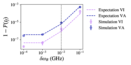
Figure 6: Spin backaction on valley evolution, as measured by median state infidelity Eq. (24) (empty circles) over a subset of 1000 different testcases, drawn randomly from the dataset considered in the main text. Error bars represent first interquartile ranges. The dashed vertical line marks the typical value of $\delta\omega_{B}\sim 10^{-2}\,$GHz, below which the infidelities saturate to the uncoupled infidelities obtained from optimization. Dashed line represents the expectations of infidelity contribution from the spin-valley coupling, given by the maximum between $(\delta\omega_{B}\tau/(2\pi))^{2}/2$ and the uncoupled infidelities.

References

- McKay et al. [2017] D. C. McKay, C. J. Wood, S. Sheldon, J. M. Chow, and J. M. Gambetta, Phys. Rev. A 96, 022330 (2017).
- [2] Supplemental Material available at URL to be inserted by publisher.
- Nielsen and Chuang [2012] M. A. Nielsen and I. L. Chuang, Quantum Computation and Quantum Information: 10th Anniversary Edition (Cambridge University Press, 2012).
- [4] M. P. Losert, M. Oberländer, J. D. Teske, M. Volmer, L. R. Schreiber, H. Bluhm, S. N. Coppersmith, and M. Friesen, arXiv:2405.01832 .
- Swinbank and James Purser [2006] R. Swinbank and R. James Purser, Quarterly Journal of the Royal Meteorological Society 132, 1769–1793 (2006).
- Gonzalez [2009] A. Gonzalez, Mathematical Geosciences 42, 49–64 (2009).