Relating dynamics and structure of
discrete and continuous time systems
Shuyun Jiao1 and David Waxman2
1Mathematics and Computer Science College,
Shanxi Normal University, 339 Taiyu Road, Taiyuan, Shanxi, 030031, PRC
2Centre for Computational Systems Biology, ISTBI,
Fudan University, 220 Handan Road, Shanghai 200433, PRC
1Email: jiaosy@sxnu.edu.cn ORCID ID: 0000-0002-4738-4668
2Email: davidwaxman@fudan.edu.cn ORCID ID: 0000-0001-9093-2108
Abstract
There are many instances, in subjects such as biology, where a population number, or related quantity, changes in discrete time. For the population number at time , written , we show that some exactly soluble cases of can be related to a different problem, where the number of individuals changes in continuous time. With the population number at continuous time , the relation is that precisely coincides with . In such a case, we call the two models equivalent, even though obeys a difference equation and obeys a differential equation. Cases of equivalence can be found for both time homogeneous and time inhomogeneous equations.
A comparison of the difference equation and the differential equation of the equivalent problem, allows us to make a correspondence between coefficients in these equations, thereby exposing structural similarities and differences of the two problems.
When the equation that obeys is modified, e.g., by the introduction of time inhomogeneity, so has no exact solution, we show how to construct an approximate equivalent continuous time solution, . We find that can yield a good approximation to because encapsulates much of the behaviour of .
We note that some discrete time problems may have solutions with an oscillatory component that changes sign as . This occurs with the Fibonacci numbers. We find that the way an equivalent continuous time solution replicates this oscillatory behaviour is by becoming complex; it no longer represents a simple interpolation.
1 Introduction
There are many instances in biology and related subjects where a population exhibits change in discrete time. Two examples that come readily to mind are: (i) an evolving biological population with non-overlapping generations, such as an annual plant [1], and (ii) the spread of a virus, within a population, when testing is carried out at regular times (such as every week), and knowledge of the number of infected individuals is known only at the times of testing [2].
These two examples have different interpretations of the discrete time-steps, but in what follows, we shall often describe discrete time-steps as generations, irrespective of the context.
Consider a population that changes in discrete time. If a mathematical model of this population can be approximated by a model that exhibits change in continuous time, then typically, much more analytical information will be available about the behaviour of the population.
A typical situation where discrete time can be well approximated by continuous time is when the dynamical quantity of interest, e.g., an gene frequency or population size/number, exhibits only small fractional (or percentage) changes from one generation to the next. Then, such an approximation can plausibly be made, and the difference equation, which describes the discrete time dynamics, becomes replaced by the corresponding continuous time description, namely a differential equation. However, what happens when changes in the dynamical quantity of interest do not have small fractional changes, from one generation to the next? In such cases, it would appear to be a very bad approximation to replace discrete time by continuous time.
In the present work we introduce methodology that, in some cases, allows us to obtain a continuous time description of a discrete time problem, that is exact in the sense that when the continuous time equals a generation time (i.e., an integer) the discrete and continuous time problems have solutions that precisely agree. We shall describe the discrete and continuous time problems, when this precise agreement occurs as being equivalent.
When such a continuous time description exists that is equivalent to a discrete time problem, we learn the generally nontrivial relationship between coefficients of terms in the discrete time problem and related coefficients in the equivalent continuous time problem. This equivalence of discrete and continuous time problems is not solely when there is time homogeneity. As we shall show in some examples, there are cases of time-dependent parameters that also lead to equivalence (i.e., exact agreement of the discrete and continuous time problems at discrete generation times).
The equivalent continuous time analogue of an exactly soluble discrete time problem can capture quite extreme behaviours of the discrete time solution, such as extremely rapid growth. We can exploit this, by considering a modification of an exactly soluble discrete time problem, so that it has no exact solution. The same (or very similar) modification of the equivalent continuous time problem, will now no longer be equivalent to the modified discrete time problem. However, this continuous time problem may serve as a useful starting point for elucidating the behaviour of the modified discrete time problem, since it may encapsulate a very large amount of the behaviour of the discrete time problem. We shall explore some examples of this approach in this work.
Beyond this, while the equivalent continuous time solution may be viewed as simply an interpolation of the discrete time solution, that precisely agrees at discrete times, this is not the full story. For some discrete time problems, there may be an oscillatory component that changes sign often. We give examples where an exactly soluble discrete time solution gives rise to an equivalent continuous time solution. However, to define this solution, we find it needs to be complex.
2 Elementary example: population growth
We shall begin by considering deterministic population growth in the absence of resource limitations. This will serve as an elementary illustrative example.
2.1 Description
Let denote the size in of a population in generation (). The equation governing the size of the population is
| (2.1) |
This describes the situation where the population size deterministically changes by a factor each generation, with size treated as a continuous non-negative quantity. Until we say otherwise, we take the parameter to be a constant. Then, when lies in the range , the population size decreases each generation, while when it increases.
A full specification of the problem needs to be subject to an initial condition. We take
| (2.2) |
where is the initial population size. The solution for is then given by
| (2.3) |
One way to motivate a continuous time approximation of Eq. (2.1) is to first write Eq. (2.1) as and then make the following changes:
(i) replace the integer-valued index by a continuous time parameter, ;
(ii) replace by a function of that we write as ;
(iii) replace the finite difference by the time derivative .
This leads to the replacement of Eq. (2.1) by the differential equation , which is subject to the same initial condition as the discrete-time problem, and has the solution .
Although the above procedure is not rigorous, it results in a good approximation when is small because the discrete and continuous time problems have smooth solutions with very similar ‘shapes’. By this we mean that on simply replacing by in the factor , which appears in the solution of the discrete time problem (Eq. (2.3)), we obtain . This has very similar behaviour, for small , to that of the corresponding factor in the solution of the continuous time problem, namely . Indeed when we have and this differs appreciably from only at very long times given by .
In this work, however, we try to do something that differs from such a direct and limited approximation procedure. In particular, given a discrete time problem, we look for a continuous time problem that has a solution , for continuous, such that when is set equal to the integer value the solution to the continuous time problem closely or precisely coincides with the corresponding value of the exact solution of the discrete time problem.
Before we look at approximations, we shall first look for a continuous time problem with solution , where exactly coincides with , i.e., with
| (2.4) |
2.2 Exact analysis, time homogeneous case
To proceed with an exact analysis of population growth, as defined by Eqs. (2.1) and (2.2), we begin with the exact solution, which is . In this solution, we replace the integer-valued generation number, , by the continuous time parameter, (with ). This leads us to define , which we now view as the solution of an unknown continuous time problem.
At first sight, we seem to have gained nothing by this procedure. By construction, when we have precisely coinciding with the values taken by the corresponding . However, by differentiating with respect to , which is possible because is continuous, we find
| (2.5) |
In addition to the above differential equation, which obeys, the solution is subject to the same initial condition as the discrete time problem, i.e., , which we now write as
| (2.6) |
With Eqs. (2.5) and (2.6) we have a fully specified continuous time problem.
It follows that with Eqs. (2.5) and (2.6) we have established a continuous time problem that represents a dynamical system with the exact property that at the discrete times the value of the continuous time solution precisely coincides with the solution of discrete time problem.
Since a finite difference is the discrete analogue of a derivative, we write Eq. (2.1) in terms of a finite difference as , and compare this equation with Eq. (2.5). We then see it is possible to write down a mapping between the parameters appearing in the ‘equivalent’ discrete and continuous time problems. That is, the parameter in the discrete time equation (Eq. (2.1)), which can be interpreted as a ‘generational growth rate’, becomes replaced by the ‘instantaneous growth rate’ in the corresponding continuous time equation (Eq. (2.5)). Thus we have the mapping
| (2.7) |
When vanishes there is no population growth in both discrete and continuous time. When is small () both and are very similar in value and so the mapping is not that informative. However, an interesting feature of the above mapping is that ‘equivalence’ of the discrete and continuous time problems does not require the parameter to be small. For example, setting , in Eqs. (2.1) and (2.5), which is definitely not a small value, does not stop the solution of Eq. (2.5) from precisely coinciding, at with the solution of Eq. (2.1), and in this special case the ‘growth rates’ and , are very different. Indeed, despite the extreme simplicity of this scenario, it could have relevance to the deterministic spread of a highly infectious disease that has a reproduction number () of , such as measles [3]. However, in continuous time, the disease spreas would be described in terms of dynamics with an instantaneous reproduction rate of , which seemingly has no relation to the value of .
In the above example, as partially summarised by Eq. (2.7 ), we have established a mapping of parameters between a problem with discrete time and one with continuous time. We next investigate how the procedure works when the parameter has time dependence.
2.3 Exact analysis, time inhomogeneous case
We now consider the case where the parameter in the population growth problem has time dependence. In particular, we now take the generalisation of Eq. (2.1) to be
| (2.8) |
The solution is
| (2.9) |
Simply replacing by in Eq. (2.9) does not obviously yield a meaningful continuous time analogue of . However there are many forms of , and hence of , where we can evaluate the sum in Eq. (2.9) in closed form, and from this find an exact expression for . For such forms of we can obtain the equivalent continuous time problem.
2.3.1 Particular example
As a particular example, we consider
| (2.10) |
with and constants. Since there is a closed form expression for we arrive at the explicit expression
| (2.11) |
Simply replacing by in Eq. (2.11) we obtain
| (2.12) |
This form of obeys with , which we can write as
| (2.13) |
Thus Eq. (2.9), with , has a solution given by , with the solution of Eq. (2.13).
2.3.2 Illustration of the particular example
The exactly soluble case of Eq. (2.10) is simple but not so simple that it is devoid of interesting behaviour. To illustrate this, we show, in Figure 1, the equivalent continuous and discrete time solutions, and , respectively, for a range of or , for a particular choice of , and .
The parameter choices adopted for Figure 1 could represent a model of a degrading environment. For small , is positive, and the population grows over time, but for sufficiently large, becomes negative and the population then declines over time. This behaviour is exhibited in Figure 1.
In Figure 2 we give a numerical test of the results, and an indication of what we should expect when things work ‘perfectly’. For , along with the choices of and used in Figure 1, we have numerically compared the error between , as calculated from the analytical formula in Eq. (2.12), and , as calculated by direct iteration of Eq. (2.8), We used the result from iteration because, in general, that is the only way to find the .
The numerically calculated error between the exact continuous time solution, and the discrete time solution that was calculated by iteration are, as shown in Figure 2, of the order of part in . This magnitude of error is attributable to machine precision or other aspects of numerical evaluation. Errors of this magnitude should thus be expected in exactly soluble problems.
2.4 Approximate analysis, time inhomogeneous case
To carry out what is generally an approximate analysis of Eq. (2.8), we start with the exact solution in Eq. (2.9). This equation involves the quantity . Using the elementary ‘mid-point’ integration rule [4]
| (2.15) |
in the reverse direction allows us to approximate by an integral:
| (2.16) |
Then Eq. (2.9) has the approximation and combining the integrals yields . We reserve the use of for the continuous function of that is exactly equivalent to , and so define the approximately equivalent solution as
| (2.17) |
which is a function of continuous time, , but it is not, generally, exactly equivalent to . We find, from Eq. (2.17), that obeys
| (2.18) |
Thus , which satisfies Eq. (2.8), has the approximation
| (2.19) |
Plausibly, when the function changes slowly with , we have that Eq. (2.18) is an approximate continuous time analogue of Eq. (2.8) and we have the generally approximate mapping
| (2.20) |
It seems likely that the solution of Eq. (2.18) has the ability to capture a lot of the behaviour of the exact solution even for values of that may be large, since for constant , Eq. (2.18) yields the exact continuous time analogue of Eq. (2.8), even for very large . However, matters are better than this. The mid-point integration rule in Eq. (2.15) works perfectly if the function in this equation, , is a linear function of , i.e., when . Since we applied the mid-point rule to the function , this means when is a linear function of the mid-point rule will be exact. Thus when the solution of Eq. (2.18) will precisely reproduce the discrete time solution at . We have already seen the exactness of this in the previous section, where was given by Eq. (2.10). We can thus say, for a linear function of , that is not an approximation but is exact, i.e., .
We now consider a example of an that illustrates the working/accuracy of Eq. (2.18) when is a nonlinear function of , so is a genuine approximation of the equivalent continuous time solution.
2.4.1 Specific nonlinear form of
We now choose the nonlinear form of to be given by
| (2.21) |
where and are independent constants. We have adopted this form of because it leads to a simple form of the approximate equivalent solution, , where the parameter primarily determines the magnitude of the solution, while the parameter controls its periodicity (see Eq. (2.22)).
For the above form for , Eq. (2.18) yields , subject to . The solution is
| (2.22) |
The solution of this example behaves periodically over time. To illustrate the behaviour, we show, in Figure 3, the form of the approximate equivalent solution, , and the discrete time solution, , that was obtained by iteration of Eq. (2.8).
From Figure 3 there appears to be very good agreement between the continuous and discrete time solutions, even though the solutions exhibit nontrivial variation, with the height of the functions ranging from to .
For the values of and , used in Figure 3, we have numerically compared the error between and , for a range of values, with the results given in Figure 4.
It is evident from Figure 4 that the errors are twelve orders of magnitudes larger than those in Figure 2. Furthermore, the errors have a tendency to increase with the value of the parameter , that influences the rate of change of the solution (see Eq. (2.22)). This is understandable: the approximate continuous time solution cannot precisely reproduce the discrete time solution when there are relatively rapid changes in . However, we see from Figure 4 that for the value adopted for figure 3 (namely ), the errors in the approximate continuous time solution are relatively small (the errors have a magnitude less than ).
3 A nonlinear problem from genetics
In this section we illustrate the above procedure, of going from discrete to continuous time, in a model from genetics.
3.1 Description
We consider a very large (effectively infinite) population of asexual organisms, that carry one gene, which can be either or (a stricter term for and is alleles, but we shall use the term gene in this work). The population has discrete generations, labelled by . The census point in a generation is taken to be the adult stage, which occurs at the beginning of a generation, immediately prior to reproduction.
The life cycle is:
(i) adults produce offspring, which may contain a mutation, in which case the gene of the offspring will differ from that of the parent;
(ii) the adults die after reproduction;
(iii) the offspring population undergoes number regulation (thinning), with the survivors constituting the adults of the next generation.
We assume each carrier of an or gene produces a total of or offspring, respectively. Thus and represent fertilities, and until we say otherwise, they are both constants.
We shall focus on the relative frequencies (or proportions) of the population that carry the different genes. Because we deal with frequencies, all results depend on the ratio of and (see Appendix A) and we define a selection coefficient, , by
| (3.1) |
The value of is a measure of the strength of selection that is acting on relative to and lies in the range . While selection coefficients in nature are typically small () [5] there are known cases of large . As an example, if is in the vicinity of , then it corresponds to near lethality of the gene [6]. To leave the analysis general, we will not make any assumptions about the value of .
Mutations are assumed to occur independently in the production of each offspring. We use to denote the probability of an gene in a parent mutating to a gene in an offspring, while is the corresponding to mutation probability.
We assume a number regulating mechanism thins the population, by randomly picking individuals, such that at the start of every generation there are a total of adults in the population. For very large , as we assume, thinning has a negligible effect on gene frequencies and we can treat the dynamics of gene frequencies as deterministic.
3.2 Exact analysis, time homogeneous case
Let represent the relative frequency (or proportion) of adults that carry the gene in generation , with the corresponding frequency of adult carriers of the gene. In Appendix A we show that obeys the equations
| (3.2) |
where
| (3.3) |
In Appendix B we discuss the weak selection (small , and ) limit of Eq. (3.2), where , , and , leading to
| (3.4) |
We proceed with Eq. (3.2), making no assumptions about parameter values. Equation (3.2), despite being a nonlinear difference equation for , can be analytically solved. In Appendix C we show that with the initial frequency, , we have
| (3.5) |
where
| (3.6) | ||||
| (3.7) |
We now replace the integer-valued generation number, , in Eq. (3.5) by the continuous time parameter, , leading us to
| (3.8) |
As before, we view as the solution of an unknown continuous time problem. On differentiating this form of with respect to , and then eliminating all dependence on the initial frequency, , we obtain the time homogeneous problem given by
| (3.9) |
and
| (3.10) | ||||
| (3.11) | ||||
| (3.12) |
We note that the coefficients of , and , in Eq. (3.9) are all constants.
Comparing Eq. (3.9) with Eq. (3.4), it is natural to interpret the coefficient of in Eq. (3.9) as playing the role of a selection coefficient in continuous time, while the coefficients of and play the corresponding role of forward and backward mutation rates, respectively. However, the real comparison is with the unapproximated discrete time genetics equation, namely Eq. (3.2), written in the form . We thus infer the exact mappings, from the frequency dependent coefficients in discrete time, to frequency independent coefficients in continuous time, are given by
| (3.13) | ||||
In the special case of , only the coefficient of is nonzero, and for this case while . Thus at order they agree, but at order there is a fundamental discrepancy in form, with one coefficient dependent, the other a constant.
We view the mapping in Eq. (3.13) as one with a nontrivial character; it is not just between parameters, but between functions with different dependence.
3.3 Exact analysis, time inhomogeneous case
We now consider a time inhomogeneous genetics problem, where there is no mutation but time-dependent selection acts. In this case we take the analogue of Eq. (3.2) to be
| (3.14) |
where, now, the selection coefficient depends on the discrete time, . In Appendix D we show that the exact solution to Eq. (3.14 ), subject to , is
| (3.15) |
There are similarities of this result with the results for population growth in Sections 2.3 and 2.4. We could replicate the sort of things we did in those sections, for example, choosing specific forms for where the sum in Eq. (3.15) can be evaluated in closed form, but we will not do so here. We will, however, approximate by an integral (again using the approximate mid point integration rule in the opposite direction):
| (3.16) |
This result allows us to write Eq. (3.15) for as
| (3.17) |
Equation (3.17) motivates defining the approximate continuous time solution
| (3.18) |
which satisfies
| (3.19) |
Comparing Eq. (3.19) with the original difference equation, Eq. (3.14), written as , leads to the (generally approximate) mapping
| (3.20) |
and as in constant case of Section 3.2, a frequency dependent coefficient (namely that of ) in the discrete time problem becomes a frequency independent coefficient in continuous time. Furthermore, the approximation in Eq. (3.16) is exact when is a linear function of . In this case, Eq. (3.19) will have a solution that precisely agrees with the solution of Eq. (3.14) when , irrespective the size of the parameters in .
4 Oscillatory and complex
It seems plausible that the method we have presented will also work for second order difference equations, such as the Fibonacci problem (see e.g., [7]), where the number of individuals in a population at time , written , takes integer values and obeys along with and . The solution is where and . We note that in this solution, the term involving is oscillatory: it changes sign as . Thus despite the fact that for the magnitude of is smaller than the other term, , possibly much smaller, the oscillatory behaviour of is a new feature that we have not so far encountered.
Indeed when we replace by , the continuous time solution represents an ambiguously specified complex solution, because of the presence of the term . We thus have to understand oscillatory problems in discrete time, and their continuous time equivalent analogues. We next study a simple problem with this feature.
4.1 A simple example of an oscillatory
Consider the discrete time problem
| (4.1) |
whose solution is
| (4.2) |
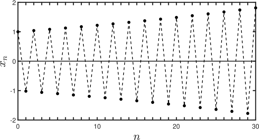
Thus if we take to be negative, say with then the solution for is
| (4.3) |
and this is oscillatory in the sense that and have different signs. We have plotted an example of against in Figure 5.
Consider the solution of the continuous time problem that is equivalent to Eq. (4.1), and obtained from Eq. (4.2 ) by replacing by :
| (4.4) |
This satisfies
| (4.5) |
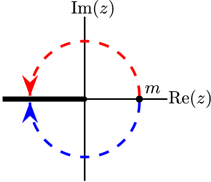
To determine what arises when we see that a way to proceed is to treat as a complex variable. We then need to ensure that both and are well-defined functions of for general (real) . This entails both of these functions having a cut along the negative real axis in the complex plane. The way to arrive at with is as follows.
With , we set
| (4.6) |
with real and lying in the range . We then take from to either or , corresponding to moving on a semicircular arc around the origin in the complex plane, from , and arriving at either or , respectively. We illustrate this procedure in Figure 6.
We find that under this procedure, Eq. (4.4) becomes
| (4.7) |
while Eq. (4.5) becomes
| (4.8) |
The two solutions in Eq. (4.7) are, for general , both complex, and indeed are complex conjugates of each other. This is also reflected in the ordinary differential equations for in Eq. (4.8); the coefficients of , on the right hand sides are also complex conjugates of each other.
We can write the two solutions in Eq. (4.7) as and for general these have both real and imaginary parts, i.e., they are intrinsically complex. However, if we set () then the imaginary parts vanish, and both solutions reduce to , precisely coinciding with the exact result in Eq. (4.3).
From the above example, we cautiously infer the following about exactly soluble discrete time problems that exhibit oscillatory behaviour (such as has a different sign to ).
-
1.
The procedure of obtaining an equivalent continuous time solution, , by replacing by in the exact discrete time solution, , continues to work, in the sense precisely coincides with .
-
2.
The way the continuous time equivalent solution, , reproduces the rapid changes in is to become complex.
-
3.
The differential equation that obeys generally has complex coefficients.
-
4.
Since there is no reason that either or is ‘adopted’ by the continuous solution, there are two equivalent continuous time solutions that precisely reproduce the value of when . These solutions are complex conjugates of each other and have an equal status, with neither preferable over the other. The two solutions also satisfy differential equations whose coefficients are complex conjugates of each other.
-
5.
When the imaginary parts of the two equivalent continuous time solutions precisely vanish, but for general the imaginary parts are non-zero.
4.2 Fibonacci second order problem
We are now in a position to return to the Fibonacci problem that we discussed at the beginning of this section.
The discrete time equation is
| (4.9) |
and the solution is
| (4.10) |
To obtain the equivalent continuous time solution, , from the above expression for we follow the approach of Section 4.1. In particular, we assume the term , that is present in Eq. (4.10), had its origin in the expression .
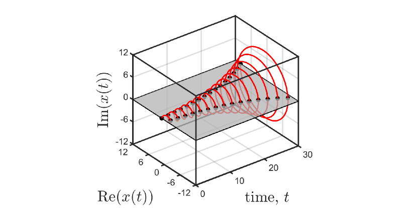
Focussing on as a function of the complex variable , we now substitute for and obtain . As in the previous section, we move , in the complex plane, now from to either or , in a similar manner to Figure 6. This leads to in Eq. (4.10) giving rise, in continuous time, to the two expressions , which are complex conjugates of each other. It then follows that the continuous time solutions, that are equivalent to , are
| (4.11) |
with and given in Eq. (4.10). In Figure 7 we have plotted the solution against .
In Appendix E we show that , as given by Eq. (4.11), obeys an ordinary differential equation with complex coefficients, and an initial condition that involves the first derivative also being complex:
| (4.12) | |||
| (4.13) |
5 Discussion
In this work we have established connections between discrete time dynamical systems and their continuous time counterparts.
We have always gone from a discrete time to continuous time, and this seems to be free of ambiguities when the discrete time solution depends analytically on . We can simply replace by to obtain a unique continuous time solution. Going the opposite way, from to seems problematic. There are many continuous time solutions that can lead to the same discrete time solution. For example , for arbitrary, leads, in discrete time to just , independent of .
We proceeded by first looking at both time homogeneous and time inhomogeneous problems that have closed form solutions of the discrete time equation, for . By the substitution we converted these exact solutions into continuous time solutions, , that are defined for . By construction, will precisely coincide with when . What is not obvious is the relation between the difference equation that obeys and the differential equation that obeys - the latter found by differentiating and eliminating initial data. When we have adopted such a procedure, we have found that there are two major cases:
(1) changes smoothly, in the sense that for most , the sign of any component of has the same sign as the corresponding component of .
(2) has at least some components that change in an oscillatory manner, i.e., a component of has a different sign to the corresponding component of .
We shall discuss these two cases separately.
-
1.
changes smoothly
-
(i)
In the cases considered, we have found that time homogeneous difference equations lead to time homogeneous differential equations.
-
(ii)
In the cases considered, we have found that time inhomogeneous difference equations lead to time inhomogeneous differential equations.
-
(iii)
Given that there is a reasonably unambiguous identification of corresponding terms in the difference and differential equations in the cases considered, we have found that in some discrete time equations, coefficients of particular terms are dependent, but in the differential equation these coefficients are constants ( independent). This indicates different functional forms for corresponding coefficients.
-
(i)
-
2.
is oscillatory
In this case, we saw an example where the discrete time equation has a part involving with . To define a continuous solution in such a case, we start with the function and have two ways, in the complex plane, to unambiguously make negative. This leads to two equal status solutions of , that are complex conjugates of each. The associated differential equations have coefficients that are complex conjugates of each other.
For Point (i), it was not obvious, at the outset, that a time homogeneous differential equation would arise.
Points (i) and (ii) mean, for example, that there can be enormous growth in with and yet there still is a continuous time solution, , that precisely yields . This can be a starting point for an approximation scheme, where a modification of cannot be solved exactly. We have presented an approach, based on an approximation of a term by an integral, where a continuous time solution can be found that may capture a lot of the behaviour of , and so be ‘close’ to for all . Indeed, in some cases the approximation leads to an exactly equivalent solution.
Point (iii) indicates potentially fundamental differences in the structure of discrete and continuous time problems. We had, in a discrete time example, a coefficient of of (see Section 3.2). The corresponding coefficient, of in continuous time, is . Thus only at first order in do and agree, but beyond this the dependence of the discrete time coefficient indicates a real difference to the continuous time coefficient. We are unsure of the full implications of this.
In Point , the ‘complexification’ of the solutions changes the picture of as an interpolation of to non discrete . Now, oscillatory do not yield a continuous time solution that interpolates the . Indeed, when is not an integer, is complex, as is illustrated in Figure .
In the case of the Fibonacci numbers, as considered in Section 4.2, as the discrete time increases, the ‘problematic’ term makes an increasingly small contribution to the full form of . In discrete time the term seems simply to correct the exponentially growing term (), to make the final result an integer. Thus a term of numerically small magnitude can have a very large effect on the nature of the equivalent continuous time solution.
We started this work by deriving a continuous time solution from a discrete time solution. From a different perspective, we could take the continuous time solution, , as describing a population with genuinely overlapping generations (when is real). Under such an interpretation, the approach presented in this work allows us to see the relation of two populations with similar numbers/frequencies, but evolving in discrete or continuous time.
The above are basic considerations of the results we have presented. Beyond this, we believe it would be particularly interesting if we could go directly from a difference equation to an equivalent or near equivalent differential equation. It would also be most interesting to consider difference equations with random coefficients. Can these be converted to a continuous time equation with a stochastic character? We note that in the realm of Fibonacci numbers, the generalisation to include random coefficients has been made [8], [9].
APPENDICES
Appendix A Representing the dynamics in the genetics model
In this appendix we determine the dynamics of a population of haploid asexual organisms that evolve in discrete generations, as considered in Section 3 of the main text.
Individuals carry one of two genes, labelled and , and in the adults of generation , with , the number of carriers of the gene and that of the genes is .
The life cycle is: (i) adults produce offspring, and if they contain a mutation then they have an gene different from the parental gene; (ii) the adults die after reproduction; (iii) the offspring undergo number regulation, leaving individuals who constitute the adults of the next generation. We assume is sufficiently large that the dynamics can be treated as deterministic.
The carrier of an gene produces a total of offspring, while a carrier of a gene produces a total of offspring.
Let denote the probability that an gene in a parent mutates to a gene in an offspring, while denotes the corresponding probability that a gene mutates to an gene.
After reproduction, we write the number of offspring carrying the and genes as and , respectively, and
After number regulation, the numbers of adults carrying the different genes in the next generation are given by
| (A.2) | ||||
where is a ‘number regulation factor’: a function of and that ensures the sum of the numbers of and gene carriers equals .
Let
| (A.3) |
denote the frequency of adult carriers of the gene in generation , with the corresponding frequency of gene carriers given by . Then from Eq. (A.2) we obtain
| (A.4) |
which can be written as
| (A.5) |
We can express this equation in the equivalent form
| (A.6) |
where
| (A.7) |
These three results can be expressed in terms of the selection coefficient defined by
| (A.8) |
We then find
| (A.9) |
Appendix B Weak selection limit of the genetics model
In this appendix, we consider the weak selection limit of the genetics model considered in the main text, given in Eqs. (3.2) and (3.3), which we reproduce here:
| (B.1) |
where
| (B.2) |
Under weak selection, corresponding to small (), we can expand in , neglecting terms of order . We obtain . If we also assume and are small, to the extent we can neglect terms of order and , then we obtain and . We then arrive at the weak selection equation
| (B.3) |
The assumed smallness of , , and suggest that this equation has solutions that are very close to the solutions of the continuous time equation
| (B.4) |
which occurs in population genetics [10].
Equation (B.1) is of a similar form to Eq. (B.3), except the coefficients of , , are the frequency-dependent quantities , , and of Eq. (B.2). This frequency dependence most strongly manifests itself under strong selection, i.e., when is not small compared with , which occurs when there is an appreciable discrepancy between and . Another way of saying this is that when carriers of different genes make significantly different inputs into a generation (due to being appreciably different to ), there is frequency dependence in coefficients that are, when selection is weak, effectively constants.
Appendix C Solution of the dynamics in the genetics model
In this appendix we derive the exact solution of the genetics problem, as described in Section 3.2 of the main text and Appendix A.
To begin, we write and and Eq. (A.5), which is equivalent to Eq. (3.2) of the main text takes the form
| (C.1) |
Let be the equilibrium solution that solves
| (C.2) |
We find the solution that lies in the range is given by
| (C.3) |
Then we can write
| (C.4) |
We set
| (C.5) |
Then find
| (C.6) |
where
| (C.7) |
The solution is
| (C.11) | ||||
| (C.15) |
leading to the exact solution for :
| (C.16) |
In terms of the selection coefficient defined by
| (C.17) |
we have
Appendix D Solution of the time inhomogeneous dynamics in the purely selective genetics model
In this appendix we determine the solution of the difference equation that occurs in Eq. (3.14) of the main text.
We find it more convenient to carry out some of the algebraic manipulations in terms of the (discrete) time dependent and , prior to expressing their ratio in terms of a time dependent selection coefficient.
In this case we take the time-dependent mutation-free analogue of Eq. (3.2) to be
| (D.1) |
We write this as
| (D.2) |
or
| (D.3) |
The solution for is
| (D.4) |
thus
| (D.5) |
With
| (D.6) |
we have
| (D.7) |
Similarly to the population growth problem, we shall approximate by an integral (again using the approximate mid point integration rule in the opposite direction to usual):
| (D.8) |
then
| (D.9) |
and we can write this for as
| (D.10) |
This leads us to define
| (D.11) |
which satisfies
| (D.12) |
The original difference equation, Eq. (D.1), can be written as
| (D.13) |
Comparing the previous two equations, we arrive at the (generally approximate) mapping
| (D.14) |
and as in the population growth case, a frequency dependent coefficient in the discrete time problem becomes a frequency independent coefficient in continuous time. Furthermore, the approximation in Eq. (D.8) is exact when is a linear function of . In this case, Eq. (D.12) will have a solution that precisely agrees with the solution of Eq. (D.13) when , irrespective the size of .
Appendix E Derivation of the differential equation in a second order problem
In this appendix we derive the differential equation obeyed by the function of given in Eq. (4.11) of the main text. The function is
| (E.1) |
where and .
The function in Eq. (E.1) arose from a second order difference equation, and to facilitate the derivation of the differential equation it obeys, we write
| (E.2) |
where we treat and as arbitrary constants that are determined by initial data, and shall look for a differential equation that is independent of and .
We have
| (E.3) | ||||
| (E.4) |
From these equations we obtain
| (E.5) | ||||
| (E.6) |
Substituting these into Eq. (E.2) yields the time homogeneous equation
| (E.7) |
Setting yields the differential equation that the function in Eq. (E.1) obeys:
| (E.8) |
which can be written in an alternative form111We can Eq. (E.8) as =0.. From Eq. (E.1) we have
| (E.9) |
References
- [1] J. M. Smith, Mathematical ideas in biology. Cambridge University Press, Cambridge, UK, 1968.
- [2] A. A. Yakubu, “A discrete-time infectious disease model for global pandemics,” Proceedings of the National Academy of Sciences, USA, vol. 19, p. 118, 2021.
- [3] F. M. Guerra, S. Bolotin, G. Lim, J. Heffernan, S. L. Deeks, Y. Li, and N. S. Crowcroft, “The basic reproduction number (R0) of measles: a systematic review,” The Lancet Infectious Diseases, vol. 17, p. e420, 2017.
- [4] A. Jeffrey, Handbook of Mathematical Formulas and Integrals (Third Edition). Academic Press, Burlington, CA, 2004.
- [5] A. Walker and P. D. Keightley, “The distribution of fitness effects of new mutations,” Nature Reviews Genetics, vol. 8, pp. 610–618, 2007.
- [6] D. Waxman and A. Overall, “Influence of dominance and drift on lethal mutations in human populations,” Frontiers in Genetics, vol. 11, p. 267, 2020.
- [7] S. Elaydi, An Introduction to Difference Equations Third Edition. Springer, NY, USA, 2005.
- [8] D. Viswanath, “Random fibonacci sequences and the number 1.13198824…,” Mathematics of Computation, vol. 69, p. 1131, 2000.
- [9] M. Embree and L. N. Trefethen, “Growth and decay of random fibonacci sequences,” Proceedings of the Royal Society London A, vol. 455, p. 2471, 1999.
- [10] T. Nagylaki, Introduction to Theoretical Population Genetics. Springer, Berlin, GER, 1992.