Mean first-passage time at the origin of a run-and-tumble particle with periodic forces

Abstract

We consider a run-and-tumble particle on a half-line with an absorbing target at the origin. The particle has an internal velocity state that switches between two fixed values at Poisson-distributed times. The particles evolves according to an overdamped Langevin dynamics, with a periodic force field, such that every in a given period interval are accessible to the particle. The Laplace transform of the backward Fokker–Planck equation satisfied by the survival probability of the particle yields systems of equation satisfied by the moments of the first-passage time of the particle at the origin. The mean first passage time has already been calculated assuming the particle reaches the origin in finite time almost surely. We calculate the probability that the particle reaches the origin at finite time, given its initial position and velocity. We obtain an integral condition on the force, under which the exit probability is less than one. If the force field is a constant drift, the condition is satisfied by positive values of the drift. The mean first-passage time of the particle (averaged over trajectories that reach the origin) is obtained in closed form as a consequence in both regimes.

1 Introduction, model and summary of results

The mean first-passage time of a particle at a target is of interest in a variety of contexts, including search behavior or execution of limit orders in finance. They have been extensively studied in the case of Brownian particles (see [1] for a review). Indeed, the first-passage problem has been an active research problem in the literature; see also [2, 3, 4, 5]. The run-and-tumble particle (or RTP) has been introduced more recently as a model of active particles such as bacteria [6, 7, 8, 9]. In this model, a particle runs in a certain direction for a certain amount of time, followed by a tumble event at which the particle takes a random velocity. A typical model to describe the motion of a particle in the one-dimensional space is the following overdamped Langevin equation:

$$\frac{dx_{t}}{dt}=F(x_{t})+v\sigma(t),$$ (1)

where $x_{t}$ is the location of the particle at time $t$, $F(x):\mathbb{R}\rightarrow\mathbb{R}$ is the external force, $v>0$ is the velocity and $\sigma(t)$ a stochastic process switching between two states $\sigma=\pm 1$ with rate $\lambda>0$. We will refer to $v\sigma(t)$ as the internal velocity state of the particle at time $t$. The total velocity of the particle at time $t$ is the sum of the internal velocity state and the value of $F$ at the position $x_{t}$ of the particle. The propagator of the free run-and-tumble particle on the real line has been computed exactly [10, 11, 12] (for developments in higher dimension, see [13]).

The survival probability of a free RTP on a half line with an absorbing point at the origin, as well the non-crossing probability of two free RTPs in dimension one, have been worked out in [14]. If the run-and-tumble particle is subjected to stochastic resetting of its position and possibly of its velocity state (at Poisson-distributed times), the system reaches a steady state that has been computed exactly [15] (see [16] for results in dimension two). Moreover, models of RTPs in dimension one in the presence of force fields and boundaries have been studied [21, 25, 19, 27, 23, 24, 26, 27], and some observables can be computed exactly.

In this paper, we will restrict ourselves to the case where there is only one absorbing boundary at $0$, and $F$ is periodic. Given the initial position of the particle on the positive half-line, we will calculate the exit probability (the probability of eventually reaching the origin, which is the complementary event to survival), and the mean exit time conditioned on exit. If there are two absorbing boundaries $a,b$ with $a<b$, and a particle starts within $[a,b]$, then in [24] the hitting probabilities for $a$ and for $b$ have been explicitly computed for general $F$. We will use this result and an argument of Markov chain to find the exit probability rigorously and explicitly in our case. The mean exit time has been computed explicitly in [23] for $F$ of some special forms which ensure almost sure exit for the particle. We will calculate the exit time averaged over trajectories that eventually reach the origin, for a periodic force field $F$. For a model with a periodic piecewise-linear potential, see [28]. Run-and-tumble particles with periodic force fields were studied in [25], where the emphasis was on the distribution of the position (and the mean first-passage time at a given level was obtained assuming reflecting boundary conditions at the end of a half-line).

More precisely, we consider a run-and-tumble particle in one dimension, characterized by Eq. (1), with velocity $v_{0}$ and tumbling rate $\gamma$. The positive half-line is endowed with a periodic force field $F$ (with period denoted by $a$), hence for any $x\geq 0$:

$$F(x+a)=F(x).$$ (2)

We want the particle to be able to reach any point in the positive half-line. The force field is therefore assumed to satisfy

$$|F(x)|<v.$$ (3)

for all $x\geq 0$ (the values of the force field are said to be subcritical). However, the above condition is not sufficient for all points within a period (including endpoints) to be accessible for a particle starting at any point in this period. We need to assume (4) and (5) below: the equation

$$\frac{dx_{t}}{dt}=F(x_{t})+v,\quad x_{0}=0,$$ (4)

has a finite time $t_{+}>0$ such that $x_{t_{+}}=a$; and the equation

$$\frac{dx_{t}}{dt}=F(x_{t})-v,\quad x_{0}=0,$$ (5)

has a finite time $t_{-}>0$ such that $x_{t_{-}}=-a$. Clearly, (4) and (5) imply (3). To our best knowledge, conditions (4) and (5) were not mentioned in the literature, but are necessary and sufficient to guarantee accessibility of all points within a period interval (including endpoints). We give a counterexample for (4). Let us define $F$ on one period interval by $F(x)=-v+a^{-1}\gamma(a-x)^{2}$ for $x\in[0,a)$, assuming $a<2v\gamma^{-1}$ for the values to bu subcritical. If the particle starts at the origin, Eq. (4) becomes

$$\frac{dx_{t}}{dt}=a^{-1}\gamma(a-x_{t})^{2},\quad x_{0}=0.$$

Solving this differential equation yields $x_{t}=a\gamma t(1+\gamma t)^{-1})$. Hence $\lim_{t\to\infty}x_{t}=a$, but will never reach $a$ and go beyond.

Assuming all points in a period interval including the endpoints are accessible, we will first study the exit probability, given a starting position $x>0$ and an internal velocity state:

$$E(x,\pm):=P({\mathrm{min}}(t,x_{t}=0)<\infty|x_{0}=x,\sigma(0)=\pm 1).$$ (6)

The exit probability satisfies the following system of equations:

$$\begin{cases}0=&(F(x)+v)\frac{\partial E(x,+)}{\partial x}+\gamma E(x,-)-\gamma E(x,+),\\ 0=&(F(x)-v)\frac{\partial E(x,-)}{\partial x}-\gamma E(x,-)+\gamma E(x,+).\end{cases}$$ (7)

We will prove that the exit probability $E(x,\pm)$ is identically equal to $1$ if the force field satisfies the integral condition

$$J(a)>0,\quad{\mathrm{with}}\quad J(x):=\gamma\int_{0}^{x}\frac{F(y)}{v^{2}-F(y)^{2}}dy.$$ (8)

Moreover, we will obtain the exit probability as

$$\begin{split}E(x+Na,\pm)=&\mathbbm{1}\left(J(a)\leq 0\right)\\ &+\left[\frac{e^{-NJ(a)}[2\Xi_{-}(a)-(1-e^{-J(a)})(2\Xi_{-}(x)\pm e^{-J(x)})]}{1-e^{-J(a)}+2\Xi_{-}(a)}\right]\mathbbm{1}\left(J(a)>0\right),\\ &{\mathrm{for}}\quad x\in[0,a[,\;\;\;\;N\in\mathbb{N},\quad{\mathrm{with}}\;\;\;\Xi_{-}(x):=v\gamma\int_{0}^{x}\frac{e^{-J(y)}}{v^{2}-F(y)^{2}}dy.\end{split}$$ (9)

The second quantity of interest is the mean exit time $T(x,\pm)$ of the particle that starts at coordinate $x$ with internal velocity state $\pm$, calculated over the configurations with finite exit times:

$$T(x,\pm)=\int_{0}^{\infty}dt\,t\Phi_{\pm}(x,t),$$ (10)

where $\Phi_{\pm}(x,t)$ is the flow density at time $t$ through the origin of a particle that was at position $x>0$ at time $0$. It satisfies the system of equations

$$\begin{cases}-E(x,+)=(F(x)+v)\frac{\partial T(x,+)}{\partial x}+\gamma T(x,-)-\gamma T(x,+),\\ -E(x,-)=(F(x)-v)\frac{\partial T(x,-)}{\partial x}-\gamma T(x,-)+\gamma T(x,+).\\ \end{cases}$$ (11)

This problem was solved in [24] for a general force field $F$, assuming the exit probabilities $E(x,\pm)$ are identically equal to $1$. In cases where the exit probability $E(x,\pm)$ is equal to 1, the quantity $T(x,\pm)$ is the mean-first passage time of the particle at the origin (given initial position and velocity state). The conditioned average over the trajectories that eventually reach the origin can be defined in all cases as

$$C(x,\pm)=\frac{T(x,\pm)}{E(x,\pm)}.$$ (12)

These conditioned averages were calculated in [17] in the case of a constant force field. In particular, if $F(x)=\mu$ for all $\geq 0$, with $\mu$ in $]-v,v[$ for all $x\geq 0$, the value of $T(0,+)$ was shown to be $(1-\mu)[\mu(1+\mu)]^{-1}$ for positive $v$, and to be $1/|\mu|$ for negative $v$. Having obtained the exit probability $E(x,\pm)$, we will solve Eq. (11) and obtain $T(x,\pm)$ for a more general periodic force field. We will show in particular that

$$\begin{split}T(0,+)=&\left[\frac{\Xi_{+}(a)}{\gamma(1-e^{J(a)})}\right]\mathbbm{1}(J(a)<0)\\ &+\left[\frac{e(0)\psi(a)-[e(0)+1]\varphi(a)}{\gamma(1-e^{-J(a)})}\right]\mathbbm{1}(J(a)>0)\\ {\mathrm{with}}\;\;\;\;E(x):=&\frac{1}{2}\left(E(x,+)+E(x,-)\right),\\ e(x):=&\frac{1}{2}\left(E(x,+)-E(x,-)\right),\\ \varphi(x):=&\gamma e^{-J(x)}\int_{0}^{x}\frac{e(y)F(y)-vE(y)}{v^{2}-F(y)^{2}}e^{+J(y)}dy,\\ \psi(x):=&2\gamma v\int_{0}^{x}\frac{\varphi(y)}{v^{2}-F(y)^{2}}dy+\gamma\int_{0}^{x}\frac{E(y)F(y)-e(y)v}{v^{2}-F(y)^{2}}dy.\end{split}$$ (13)

The paper is organized as follows. In Section 2 we review the backward Fokker–Planck equation satisfied by the survival probability of an RTP in a force field with subcritical values and satisfying (4) and (5). Taking the Laplace transform induces the systems of differential equations presented in Eqs (7,11). In Section 3 we restrict ourselves to periodic force fields, and work out a condition (expressed in terms over an integral over a period) on which the exit time is almost surely finite. We solve Eq. (7) and obtain the result reported in Eq. (9). In Section 4, we solve Eq. (11), working separately in the regimes $J(a)<0$ and $J(a)>0$. The periodicity of the force field is used to obtain a boundary condition: indeed a particle in a positive velocity state sees the same system whether it is at position $0$ or at position $a$ (the other boundary condition is more general as a particle passing at $x=0$ in a negative velocity state leaves the system immediately). We obtain the value of $T(0,+)$ reported in Eq. (13), as well as a closed-form expression of $T(x,\pm)$. The calculated functions are evaluated explicitly in the case of a piecewise constant drift taking to opposite values.

2 Notations and quantities of interest

Consider a run-and-tumble particle on the positive half-line, starting at position $x>0$, with a given internal velocity state $\pm v$. The particle undergoes Poisson-distributed tumble events. At each tumble event, the internal velocity state flips instantaneously. The rate of the corresponding Poisson process is called the tumbling rate and denoted by $\gamma>0$. The particle is said to be alive as long as its coordinate is positive. If the particle reaches the origin, the process stops. The time (if any) at which the particle reaches the origin, is called the exit time.

Let us assume that the positive half-line $F$ is endowed with a force field satisfying (4) and (5), which implies (3). Under this assumption, the total velocity of the run-and-tumble particle, which is the sum $F(x)+v$, is nonzero for the entire duration of the process. Moreover, the sign of the velocity of the particle $F(x_{t})+v\sigma(t)$ is the same as the sign of the internal velocity state at all times.

Consider the survival probability $S_{\pm}(x,t)$ at time $t$ of a run-and-tumble particle that was at position $x$ in the internal velocity state $\pm v$ at time $0$. This survival probability satisfies a backward Fokker–Planck equation [29, 30], which is derived as follows. For a particle that is alive at time $t$, and has been at position $x>0$ at time $0$ in the internal velocity state $\pm$, consider the time interval $[0,dt]$, where $dt$ is an infinitesimal time. If there is no tumble event in this interval (which is the case with probability $1-\gamma dt$), the particle is at position $x+[F(x)\pm v]dt$ at time $dt$. It must survive for a duration of time $t-dt$ to be alive at time $t$. If there is a tumble event in the interval $[0,dt]$ (which is the case with probability $\gamma dt$), the internal velocity state flips, and the particle has to survive until time $t$. Hence the two terms in the expression of the survival probability $S_{\pm}(x,t)$:

$$S_{\pm}(x,t)=(1-\gamma dt)S_{\pm}(x+[F(x)\pm v]dt,t-dt)+\gamma dtS_{\mp}(x,t).$$ (14)

Taylor expansion yields

$$S_{\pm}(x,t)=S_{\pm}(x,t)+[F(x)\pm v]dt\partial_{x}S_{\pm}(x,t)-dt\partial_{t}S_{\pm}(x,t)-\gamma dtS_{\pm}(x,t)+\gamma dtS_{\mp}(x,t),\\$$ (15)

hence the evolution equation satisfied by the survival probability on the positive half-line:

$$\partial_{t}S_{\pm}(x,t)=[F(x)\pm v]\partial_{x}S_{\pm}(x,t)-\gamma S_{\pm}(x,t)+\gamma S_{\mp}(x,t),\quad\quad(x>0,t\geq 0).\\$$ (16)

Let us denote by $\Phi_{\pm}(x,t)$ the density of first-passage time at the origin with a negative total velocity of a particle that started its motion at position $x$ in the internal velocity state $\pm v$. This density is related to the survival probability by the two equivalent equations

$$\begin{split}S_{\pm}(x,t)=&1-\int_{0}^{t}\Phi_{\pm}(x,z)dz,\\ \Phi_{\pm}(x,t)=&-\frac{\partial S_{\pm}(x,t)}{\partial t}.\\ \end{split}$$ (17)

With this definition, $\Phi_{+}(0,0)=0$ because the total velocity of a particle that is at zero at time $0$ in a positive internal velocity state is $F(0)+v$ (the particle does not exit the half-line at time $0$). Differentiating Eq. (16) w.r.t. $t$ yields a system of coupled evolution equations for the densities $\Phi_{+}$ and $\Phi_{-}$:

$$\begin{split}\partial_{t}\Phi_{\pm}(x,t)=&[F(x)\pm v]\partial_{x}\Phi_{\pm}(x,t)-\gamma\Phi_{\pm}(x,t)+\gamma\Phi_{\mp}(x,t).\\ \end{split}$$ (18)

Let us take the Laplace transform of Eq. (18), denoting the Laplace transform of the flow through the origin.

$$\tilde{\Phi}_{\pm}(x,s):=\int_{0}^{\infty}dte^{-st}\Phi_{\pm}(x,t).$$ (19)

Taking the Laplace transform of Eq. (18) (assuming $e^{-st}\Phi(x,t)$ goes to zero when $t$ goes to infinity), yields the following system of equations for $\tilde{\Phi}_{\pm}(x,s)$ (with $x>0$

$$s\tilde{\Phi}_{\pm}(x,s)=[F(x)\pm v]\partial_{x}\tilde{\Phi}_{\pm}(x,s)-\gamma\tilde{\Phi}_{\pm}(x,s)+\gamma\tilde{\Phi}_{\mp}(x,s).$$ (20)

We have used the fact that $\Phi_{\pm}(x,0)=0$ for $x>0$ (the particle does not reach the origin at time zero if it is at $x>0$).

Borrowing the notations of [24], let us denote by $E(x,\pm)$ the probability that a particle starting its motion at time $0$ at position $x$ and velocity $\pm v$ exits the positive half-line in finite time

$$E(x,\pm)=\int_{0}^{\infty}dz\Phi_{\pm}(x,z)=\tilde{\Phi}_{\pm}(x,0).$$ (21)

This exit probability appears at order $0$ in the Taylor expansion of $\tilde{\Phi}_{\pm}(x,s)$ as

$$\begin{split}\tilde{\Phi}_{\pm}(x,s):=&\int_{0}^{\infty}dt\,t\Phi_{\pm}(x,t)+o(s)\\ =&E(x,\pm)-sT(x,\pm)+o(s),\end{split}$$ (22)

where

$$T(x,\pm):=\int_{0}^{\infty}dt~{}t\Phi_{\pm}(x,t).$$ (23)

is the mean exit time (given that the particle exits after having started at $x$ in the velocity state $\pm$).

Collecting the terms of order $0$ in $s$ in Eq. (20) yields a coupled system of evolution equations for the probability of exit in finite time, given the initial velocity state:

$$\begin{split}0=&(F(x)+v)\frac{\partial E(x,+)}{\partial x}+\gamma E(x,-)-\gamma E(x,+),\\ 0=&(F(x)-v)\frac{\partial E(x,-)}{\partial x}-\gamma E(x,-)+\gamma E(x,+).\end{split}$$ (24)

Collecting the terms of order $1$ in $s$ yields a coupled system of evolution equation for the mean exit times:

$$\begin{split}-E(x,+)=&(F(x)+v)\frac{\partial T(x,+)}{\partial x}+\gamma T(x,-)-\gamma T(x,+),\\ -E(x,-)=&(F(x)-v)\frac{\partial T(x,-)}{\partial x}-\gamma T(x,-)+\gamma T(x,+).\\ \end{split}$$ (25)

These are the two systems of equations announced in the introduction in Eqs (7,11).

3 Exit probability in a periodic force field with subcritical values

3.1 Integration of the evolution equations

For brevity, let us use $\gamma^{-1}$ as the unit of time and the mean free path $v\gamma^{-1}$ as the unit of length. The period of the force field $F$ is still denoted by $a$. The periodic force field $F$ takes only subcritical values, which in these units we can summarize as $F(x+a)=F(x)$ and $|F(x)|<1$ for all $x$.

In these units, the evolution equation for the probability of exit in finite time (Eq. (7)) becomes

$$\begin{split}0=&(F(x)+1)\frac{\partial E(x,+)}{\partial x}+E(x,-)-E(x,+),\\ 0=&(F(x)-1)\frac{\partial E(x,-)}{\partial x}-E(x,-)+E(x,+).\\ \end{split}$$ (26)

Let us introduce the linear combinations, borrowing again the notations of [22]:

$$\begin{split}E(x):=\frac{1}{2}\left(E(x,+)+E(x,-)\right),\\ e(x):=\frac{1}{2}\left(E(x,+)-E(x,-)\right).\\ \end{split}$$ (27)

In terms of these unknowns, Eq. (26) becomes

$$\begin{split}0=&F(x)E^{\prime}(x)+e^{\prime}(x),\\ 0=&F(x)e^{\prime}(x)+E^{\prime}(x)-2e(x).\\ \end{split}$$ (28)

Multiplying the second equation in the system by $F$ and substituting yields a differential equation of order one in $e$,

$$0=e^{\prime}(x)+\frac{2F(x)}{1-F(x)^{2}}e(x),$$ (29)

which holds on the entire positive half-line because because the values of $F$ are subcritical. Integrating yields

$$e(x)=e(0)\exp(-J(x)),$$ (30)

with the notation

$$\begin{split}J(x):=&\int_{0}^{x}\frac{2F(u)}{1-F(u)^{2}}du.\end{split}$$ (31)

Substituting into Eq. (28) we obtain

$$\begin{split}E^{\prime}(x)=&-\frac{2e(0)}{F(x)^{2}-1}\exp\left(-J(x)\right),\\ \end{split}$$ (32)

which upon integration yields

$$\begin{split}E(x)=&E(0)+2e(0)\Xi_{-}(x),\\ \end{split}$$ (33)

with the notation

$$\begin{split}\Xi_{\pm}(x):=&\int_{0}^{x}\frac{e^{\pm J(y)}}{1-F(y)^{2}}dy\\ \end{split}$$ (34)

3.2 Boundary conditions

We need two boundary conditions to fix the constants $E(0)$ and $e(0)$. A particle starting at position $0$ in a negative internal velocity state leaves the system immediately because $F(0)-1<0$. Hence

$$E(0,-)=1,$$ (35)

which in terms of the integration constants $e(0)$ and $E(0)$ reads

$$E(0)-e(0)=1.$$ (36)

As the force field $F$ is a periodic function of period $a$, the expression of $e(x)$ in Eq. (30) induces

$$e(x+Na)=e^{-NJ(a)}e(x),\;\;\;\;\;\;(N\in\mathbb{N}).$$ (37)

The function $e$ is a linear combination of probabilities, it is therefore bounded. If $J(a)<0$, this implies that $e(x)$ is identically zero, meaning $e(0)=0$. In this case, the expression of $E(x)$ in Eq. (33) implies that the function $E$ is a constant. This constant is equal to $1$ because of the boundary condition of Eq. (36).

If $J(a)=0$, then $J(ka)=0$ for any integer $k\geq 1$. Then by Eq. (34),

$$\Xi_{-}(ka):=k\int_{0}^{a}\frac{e^{-J(y)}}{1-F(y)^{2}}dy\xrightarrow[]{k\to\infty}\infty.$$ (38)

As the function $E$ expressed in (33) in terms of the function $\Xi_{-}$ is bounded, $e(0)$ must be equal to zero. The boundary condition of Eq. (36) again implies that the RTP exits the positive half-line in finite time almost surely.

From now on let us assume that $J(a)>0$. Consider a particle starting in a positive internal velocity state at position $a$ in a positive internal velocity state (its position at time $0$ is $a$, and its velocity is $F(a)+1>0$). To exit the positive half-line, the particle must come back to $a$. It does so with probability $E(0,+)$ because the periodic system on the half line $[a,\infty[$ is the same as on the half line $[0,\infty[$. When the particle comes back to $a$, it is in a negative internal velocity state. The probability of exit from the system therefore satisfies

$$E(a,+)=E(0,+)E(a,-).$$ (39)

In terms of the unknown functions $e$ and $E$, the above condition reads

$$\begin{split}E(a)+e(a)=&(E(0)+e(0))(E(a)-e(a))\\ \end{split}$$ (40)

Using the boundary condition of Eq. (36) at the origin, and the expressions of $E(a)$ in terms of $E(0)$ and $e(0)$ in Eq. (33),

$$\begin{split}E(0)=&1+e(0),\\ E(a)=&E(0)+2e(0)\Xi_{-}(a),\end{split}$$ (41)

the boundary condition of Eq. (40) becomes an equation in $e(0)$

$$\begin{split}1+e(0)(1+2\Xi_{-}(a)+e^{-J(a)})=&[1+2e(0)][1+e(0)(1+2\Xi_{-}(a)-e^{-J(a)})],\\ e(0)(-2+2e^{-J(a)})=&2e(0)^{2}(1-e^{-J(a)}+2\Xi_{-}(a)).\end{split}$$ (42)

There are two solutions to the above equation. One is $0$ (if $e(0)=0$, we know that the particle exits the system in finite time almost surely). The other solution is negative. We will now show that under the assumption $J(a)>0$ the integration constant $e(0)$ is equal to the negative solution.

Theorem 1.

If $J(a)>0$,

$$e(0)=-\frac{1-e^{-J(a)}}{1-e^{-J(a)}+2\Xi_{-}(a)}.$$ (43)

Proof.

We just need to show that if $J(a)>0$ and the particle starts at point zero with the positive velocity, then the particle stays forever in the positive half-line with a strictly positive probability. The trajectory of the particle is continuous, but we will consider that the particle is living on the points $\{ka\}_{k\in\mathbb{Z}}$ in the sense that the trajectory of an RTP on the real line can be mapped to a Markov chain. If a particle is at position $ka$ in a positive velocity state, then it will either return to $ka$ with negative velocity or move to $(k+1)a$ with positive velocity, before getting out of $[ka,(k+1)a]$; if the particle is at $ka$ in a negative velocity, then it either returns to $ka$ with the positive velocity or move to $(k-1)a$ with negative velocity, before getting out of $[(k-1)a,ka]$. These alternatives allow us to introduce a Markov chain $(X_{n})_{n\geq 1}$ such that $X_{n}$ takes value either $1$ or $-1$.

We define the first step of the construction at time $0$, assuming that the particle is at position $0$ (it can be either in a positive or negative velocity state). In step $2$, the particle either moves to $a$ (resp. $-a$) or returns to $0$ if the velocity in step 1 is positive (resp. negative). All other steps can be done similarly. We write $X_{n}=1$ (resp. $X_{n}=-1$) if at step $n$ the particle has positive (resp. negative) velocity. Since $F$ is periodic, $(X_{n})_{n\geq 1}$ is a Markov chain. By the correspondence between living on the real line and living on $\{ka\}_{k\in\mathbb{Z}}$, we have

$$\begin{split}&\{\text{The particle stays forever in the positive half line starting from zero with positive velocity}\}\\ =&\left\{\forall k\geq 1,\sum_{i=1}^{k}X_{i}>0\,\Big{|}\,X_{1}=1\right\}.\end{split}$$ (44)

We just need to show that

$$P\left(\forall k\geq 1,\sum_{i=1}^{k}X_{i}>0\,\Big{|}\,X_{1}=1\right)>0.$$ (45)

Let $n\geq 1$ be any integer. If we write

$$p_{1,1}:=\mathbb{P}(X_{n+1}=1\,|\,X_{n}=1),\quad p_{1,-1}:=1-p_{1,1}=\mathbb{P}(X_{n+1}=-1\,|\,X_{n}=1),$$

and

$$p_{-1,1}:=\mathbb{P}(X_{n+1}=1\,|\,X_{n}=-1),\quad p_{-1,-1}:=1-p_{-1,1}=\mathbb{P}(X_{n+1}=-1\,|\,X_{n}=-1).$$

Then the transition matrix of the Markov chain is fully determined by $p_{i,j}$ for all $i,j=1,-1$. Note that $p_{i,j}>0$ for any $i,j=1,-1$, thanks to Eqs (3), (4) and (5). Therefore, $(X_{n})_{n\geq}$ is a finite-state irreducible Markov chain with a unique invariant measure, which we will denote by $\pi=(\pi_{1},\pi_{2}).$ Let us calculate the values $p_{i,j}$ and $\pi_{1},\pi_{2}$.

Let

$$Z:=A+B+1,$$

with

$$A=2\int_{0}^{a}\Xi_{-}(x)dx,\quad B=e^{-J(a)}.$$ (46)

In [24], the exit probability of an RTP from a segment has been worked out (in units of space and time where the velocity of the particle is $v_{0}$ and the tumbling rate is $\gamma$). The results of [24, (16)] yield the entries of the transition matrix of the Markov chain in our notations as

$$p_{1,1}=\frac{2}{Z},\quad p_{1,-1}=\frac{Z-2}{Z},\quad p_{-1,1}=\frac{A-B+1}{Z},\quad p_{-1,-1}=\frac{2B}{Z}.$$ (47)

The invariant measure $\pi$ satisfies

$$(\pi_{1},\pi_{2})\begin{pmatrix}p_{1,1}&p_{1,-1}\\ p_{-1,1}&p_{-1,-1}\end{pmatrix}=(\pi_{1},\pi_{2}).$$

The above equation yields

$$\pi_{1}=\frac{A-B+1}{2A},\quad\pi_{2}=\frac{A+B-1}{2A}.$$

Since $J(a)>0$, we have $B=e^{-J(a)}<1$. Then $\pi_{1}>\pi_{2}$. By the Ergodic Theorem for finite-state irreducible Markov chains [31, Theorem 1.10.2],

$$\frac{\sum_{i=1}^{n}X_{i}}{n}\xrightarrow[]{n\to\infty}\pi_{1}-\pi_{2}>0,\quad\text{almost surely.}$$

for any initial distribution of $X_{1}$. The above display implies that $\sum_{i=1}^{k}X_{i}=0$ can occur only for a (random) finite number of $k$’s. Therefore, (45) must hold, which concludes the proof. ∎

In the case $J(a)<0$, (33) therefore implies that $E$ is a strictly decreasing function of the starting position $x$. In particular, the exit probability is not identically equal to $1$.

To sum up, taking into account Eqs (30), (33) and (43), the functions $e$ and $E$ are expressed as follows:

$$\begin{split}E(x)=&\mathbbm{1}(J(a)\leq 0)+\left[\frac{2\Xi_{-}(a)-2(1-e^{-J(a)})\Xi_{-}(x)}{1-e^{-J(a)}+2\Xi_{-}(a)}\right]\mathbbm{1}(J(a)>0),\\ e(x)=&-\frac{1-e^{-J(a)}}{1-e^{-J(a)}+2\Xi_{-}(a)}e^{-J(x)}\mathbbm{1}(J(a)>0).\end{split}$$ (48)

From the definition of the unknowns in Eq. (27), the exit probability given the initial internal velocity state is expressed as follows:

$$E(x,\pm)=\mathbbm{1}(J(a)\leq 0)+\left[1-\frac{(1-e^{-J(a)})[1+2\Xi_{-}(x)\pm e^{-J(x)}]}{1-e^{-J(a)}+2\Xi_{-}(a)}\right]\mathbbm{1}(J(a)>0).$$ (49)

The integral expressions $J$ and $\Xi_{-}$ need only be evaluated on the interval $[0,a[$. Periodicity can then be used to work out the value of the exit probability at any point on the positive half-line. Substituting the expressions worked out in Eqs (112,113) of the Appendix yields

$$\begin{split}E&(x+Na,\pm)=\mathbbm{1}(J(a)\leq 0)\\ &+\left[1-\frac{2\Xi_{-}(a)+1-e^{-J(a)}+e^{-NJ(a)}[(1-e^{-J(a)})(2\Xi_{-}(x)\pm e^{-J(x)})-2\Xi_{-}(a)]}{1-e^{-J(a)}+2\Xi_{-}(a)}\right]\mathbbm{1}(J(a)>0)\\ &=\mathbbm{1}(J(a)\leq 0)+\left[\frac{e^{-NJ(a)}[2\Xi_{-}(a)-(1-e^{-J(a)})(2\Xi_{-}(x)\pm e^{-J(x)})]}{1-e^{-J(a)}+2\Xi_{-}(a)}\right]\mathbbm{1}(J(a)>0),\\ &\quad(x\in[0,a[,\;\;\;\;N\in\mathbb{N}).\end{split}$$ (50)

To restore the original, dimensionful system of units, one substitutes the symbol $x\gamma/v$ to the symbol $x$, and the symbol $F/v$ to the symbol $F$. These operations yields the result reported in Eq. (9).

3.3 Examples

3.3.1 Constant drift

As a check, let us work out the case of a constant subcritical drift $\mu$, which was solved in [17]. The functions $J$ and $\Xi_{-}$ are readily evaluated as

$$J(x)=\frac{2\mu x}{1-\mu^{2}},\;\;\;\;\quad\quad\Xi_{-}(x)=\frac{1}{2\mu}\left(1-e^{-\frac{2\mu x}{1-\mu^{2}}}\right).$$ (51)

$\bullet$ Negative subcritical drift, $-1<\mu<0$. In this case, $J(a)<0$ and the particle leaves the system almost surely.

$\bullet$ Positive subcritical drift, $0<\mu<1$. In this case, $J(a)>0$ and

$$\begin{split}\frac{2\Xi_{-}(a)}{1-e^{-J(a)}}=&\frac{1}{\mu},\;\;\;\;\;\;e(0)=-\frac{\mu}{1+\mu},~{}\;\;\;\;\;\;E(0)=\frac{1}{1+\mu},\\ e(x)=&-\frac{\mu}{1+\mu}e^{-\frac{2\mu x}{1-\mu^{2}}},\\ E(x)=&\frac{1}{1+\mu}-2\frac{\mu}{1+\mu}\Xi_{-}(x)=\frac{1}{1+\mu}e^{-\frac{2\mu x}{1-\mu^{2}}}.\end{split}$$ (52)

Hence

$$\begin{split}E(x,+)=&\frac{1-\mu}{1+\mu}e^{-\frac{2\mu x}{1-\mu^{2}}},\\ E(x,-)=&e^{-\frac{2\mu x}{1-\mu^{2}}}.\end{split}$$ (53)

This reproduces the result of [17] (Eqs (45a) and (45b) there), obtained from the the long-time limit of the survival probability on an RTP on the positive half-line with a constant positive subcritical drift.

3.3.2 Alternating drifts

A simple periodic modification of the model with constant drift worked out in [17] is the one-parameter family of alternating positive and negative drifts with the same amplitude:

$$\begin{split}F(x+Na)=&\mu I_{[0,a(1-\epsilon)]}(x)-\mu I_{]a(1-\epsilon),a[}(x),\;\;\;\;\;\;\;(x\in[0,a[,\;\;\;\;\;N\in\mathbb{N}).\end{split}$$ (54)

The function $J$ is evaluated on $[0,a[$ by calculating an integral:

$$\begin{split}J(x)=&\alpha xI_{[0,a(1-\epsilon)[}(x)+\alpha(-x+2a(1-\epsilon))I_{[a(1-\epsilon),a]}(x),\;\;\;\;\;\;\quad(x\in[0,a]),\\ {\mathrm{with}}&\;\;\;\;\;\alpha:=\frac{2\mu}{1-\mu^{2}}.\end{split}$$ (55)

In particular,

$$J(a)=\frac{2\mu}{1-\mu^{2}}a(1-2\epsilon).$$ (56)

The case of a constant drift corresponds to $\epsilon=0$, and $J(a)$ is of the sign of $\mu$ if $\epsilon<1/2$.

Calculating yields for $n=\pm 1$

$$\begin{split}\Xi_{n}(x)=&\frac{1}{2n\mu}\left(e^{n\alpha x}-1\right)I_{[0,a(1-\epsilon)[}(x)\\ &+\frac{1}{2n\mu}\left(2e^{n\alpha a(1-\epsilon)}-1-e^{2n\alpha a(1-\epsilon)}e^{-n\alpha x}\right)I_{[a(1-\epsilon),a]}(x),\;\;\;\;\;\;(0\leq x\leq a).\end{split}$$ (57)

In particular,

$$\begin{split}\Xi_{n}(a)=&\frac{1}{2n\mu}\left[e^{n\alpha a}(2e^{-n\alpha a\epsilon}-e^{-2n\alpha a\epsilon})-1\right].\end{split}$$ (58)

In particular, if $\epsilon=0$

$$\frac{\Xi_{-}(a)}{1-e^{-J(a)}}=\frac{1}{2\mu}.$$ (59)

Substituting into Eq. (50), the probability of exit for a particle starting at the origin in a positive internal velocity state is obtained as a function of the parameter $\epsilon$:

$$\begin{split}E(0,+)=&\mathbbm{1}\left(\epsilon\geq\frac{1}{2}\right)+\left[\frac{1-\frac{1-e^{-J(a)}}{2\Xi_{-}(a)}}{1+\frac{1-e^{-J(a)}}{2\Xi_{-}(a)}}\right]\mathbbm{1}\left(\epsilon>\frac{1}{2}\right)\\ =&\mathbbm{1}\left(\epsilon\geq\frac{1}{2}\right)+\frac{1-\mu\left(\frac{1-e^{-\alpha a(1-2\epsilon)}}{1-e^{-\alpha a}(2e^{\alpha a\epsilon}-e^{2\alpha a\epsilon})}\right)}{1+\mu\left(\frac{1-e^{-\alpha a(1-2\epsilon)}}{1-e^{-\alpha a}(2e^{\alpha a\epsilon}-e^{2\alpha a\epsilon})}\right)}\mathbbm{1}\left(0\leq\epsilon<\frac{1}{2}\right).\end{split}$$ (60)

This probability of exit is plotted on Fig. 1. One notices that for a fixed value of $\mu$, the limit where the period $a$ is small compared to $\alpha^{-1}=(1-\mu^{2})/(2\mu)$ yields a function of $\epsilon$ only:

$$E(0,+)\underset{a\ll 1}{\sim}\frac{1-\mu(1-2\epsilon)}{1+\mu(1+2\epsilon)}.$$ (61)

which is identical to the probability of exit in an effective constant drift $\mu(1-2\epsilon)$. On the other hand, in the limit where the period is long compared to $\alpha^{-1}$, the probability of exit goes to $(1-\mu)/(1+\mu)$ at fixed $\epsilon$, which the value obtained in the case of a constant positive subcritical drift (see Eq. (53) for $x=0$). This is consistent with intuition, as the limit of large $a$, the particle is unlikely to explore a region of space where the drift is negative.

Figure 1: The probability of exit $E(0,+)$ for a particle starting at the origin in an internal positive velocity state, for a drift alternating between $\mu=1/2$ on $[0,a(1-\epsilon)[$ and $-\mu$ on $[a(1-\epsilon),a[$, as a function of $\epsilon$. For any value of the period $a$, the limit of $E(0,+)$ when $\epsilon$ goes to zero is $(1-\mu)/(1+\mu)=3/5$.

4 First-passage time at the origin

If the mean free path of the RTP is taken as the unit of length and the internal velocity is taken as the unit of velocity, Eq. (25) becomes

$$\begin{split}-E(x,+)=&(F(x)+1)\frac{\partial T(x,+)}{\partial x}+T(x,-)-T(x,+),\\ -E(x,-)=&(F(x)-1)\frac{\partial T(x,-)}{\partial x}-T(x,-)+T(x,+),\\ \end{split}$$ (62)

where the exit probabilities in the l.h.s. have been worked out in the previous section.

Changing unknowns to

$$\begin{split}T(x):=&\frac{1}{2}\left(T(x,+)+T(x,-)\right),\\ t(x):=&\frac{1}{2}\left(T(x,+)-T(x,-)\right),\end{split}$$ (63)

and taking the sum and difference of the above equations yields a coupled system of differential equations:

$$\begin{split}-E(x)=&F(x)T^{\prime}(x)+t^{\prime}(x),\\ -e(x)=&F(x)t^{\prime}(x)+T^{\prime}(x)-2t(x).\\ \end{split}$$ (64)

Combining and substituting in the same way as above yields

$$t^{\prime}(x)+\frac{2F(x)}{1-F(x)^{2}}t(x)=\frac{-E(x)+e(x)F(x)}{1-F(x)^{2}},$$ (65)

$$T^{\prime}(x)=\frac{2t(x)}{1-F(x)^{2}}+\frac{-e(x)+E(x)F(x)}{1-F(x)^{2}}.$$ (66)

4.1 First-passage time at the origin with almost-sure exit ($J(a)<0$)

Let us assume $J(a)<0$. In this case $E(x)$ is identically equal to 1 and $e(x)$ is identically equal to 0.

Using the integrating factor $e^{J}$ we obtain

$$\frac{d}{dx}\left(e^{J(x)}t(x)\right)=-\frac{e^{J(x)}}{1-F(x)^{2}},$$ (67)

$$\begin{split}t(x)=&t(0)e^{-J(x)}-e^{-J(x)}\int_{0}^{x}\frac{e^{J(y)}}{1-F(y)^{2}}dy\\ =&t(0)e^{-J(x)}-e^{-J(x)}\Xi_{+}(x).\end{split}$$ (68)

Integrating Eq. (66) therefore yields

$$\begin{split}T(x)=&T(0)+\int_{0}^{x}\frac{2t(v)+F(v)}{1-F(v)^{2}}dv\\ =&T(0)+2t(0)\int_{0}^{x}\frac{e^{-J(v)}}{1-F(v)^{2}}dv-2\int_{0}^{x}\frac{e^{-J(v)}}{1-F(v)^{2}}\left[\int_{0}^{v}\frac{e^{J(u)}}{1-F(u)^{2}}du\right]dv+\int_{0}^{x}\frac{F(v)}{1-F(v)^{2}}dv\\ =&T(0)+2t(0)\Xi_{-}(x)-2\int_{0}^{x}dv\Xi_{-}^{\prime}(v)\Xi_{+}(v)dv+\frac{1}{2}J(x).\end{split}$$ (69)

To fix the constants we need boundary conditions. The particle leaves the system immediately if it starts at the origin with negative velocity:

$$T(0,-)=0.$$ (70)

A second boundary condition can be obtained using the periodicity of the system. If the process starts at $a$ (at the end of a period of the force field), with positive velocity. By assumption the particle reaches the origin. To reach the origin, it must first come back to $a$ (which it does with negative velocity). Moreover, the system in which the particle lives before its first return at $a$ is a half-line equipped with a periodic force field, identical to the entire system on the half-line $[0,\infty[$. Hence the additional boundary condition

$$T(a,+)=T(0,+)+T(a,-).$$ (71)

In terms of the unknowns $T$ and $t$, the boundary conditions of Eqs (70,71) imply

$$T(0)=t(0)=t(a).$$ (72)

Solving the equation $t(a)=t(0)$ using the expression of the function $t$ given in Eq. (68) yields

$$t(0)=-\frac{e^{-J(a)}}{1-e^{-J(a)}}\Xi_{+}(a),$$ (73)

which is the first term of the r.h.s. in Eq. (13), provided the symbol $\gamma^{-1}t(0)$ is substituted to the symbol $t(0)$, to express time in a system of units in which the tumbling rate equals $\gamma$.

This integration constant yields the expressions of the functions $t$ and $T$ as

$$\begin{split}t(x)=&-e^{-J(x)}\left[\frac{e^{-J(a)}}{1-e^{-J(a)}}\Xi_{+}(a)+\Xi_{+}(x)\right],\\ T(x)=&-\frac{e^{-J(a)}}{1-e^{-J(a)}}\Xi_{+}(a)\left[1+2\Xi_{-}(x)\right]-2\int_{0}^{x}dv\Xi_{-}^{\prime}(v)\Xi_{+}(v)dv+\frac{1}{2}J(x).\end{split}$$ (74)

The mean first-passage times given the initial velocity state are therefore obtained as

$$\begin{split}T(x,\pm)=&\frac{e^{-J(a)}}{1-e^{-J(a)}}\Xi_{+}(a)\left[-1-2\Xi_{-}(x)\mp e^{-J(x)}\right]\\ &-2\int_{0}^{x}dv\Xi_{-}^{\prime}(v)\Xi_{+}(v)dv+\frac{1}{2}J(x)\mp e^{-J(x)}\Xi_{+}(x).\\ \end{split}$$ (75)

Substituting the expressions obtained in the Appendix (Eqs (113,116) using periodicity yields:

$$\begin{split}T(x+Na,\pm)=&\frac{e^{-J(a)}}{1-e^{-J(a)}}\Xi_{+}(a)\left[-1\mp e^{-NJ(a)}e^{-J(x)}-2\frac{1-e^{-NJ(a)}}{1-e^{-J(a)}}\Xi_{-}(a)-2e^{-NJ(a)}\Xi_{-}(x)\right]\\ &-2\left[\frac{\Xi_{+}(a)\Xi_{-}(a)}{1-e^{J(a)}}\left(-N+\frac{1-e^{-NJ(a)}}{1-e^{-J(a)}}\right)+N\int_{0}^{a}\Xi^{\prime}_{-}(v)\Xi_{+}(v)dv\right.\\ &\left.-\frac{1-e^{-NJ(a)}}{1-e^{J(a)}}\Xi_{+}(a)\Xi_{-}(x)+\int_{0}^{x}\Xi^{\prime}_{-}(v)\Xi_{+}(v)dv\right]\\ &+\frac{1}{2}\left(NJ(a)+J(x)\right)\mp e^{-NJ(a)+J(x)}\left[\frac{1-e^{NJ(a)}}{1-e^{J(a)}}\Xi_{+}(a)+e^{NJ(a)}\Xi_{+}(x)\right],\\ &\qquad\qquad(x\in[0,a[,N\in\mathbb{N}).\end{split}$$ (76)

The leading term at large $N$ in the above expression is of order $e^{-NJ(a)}$:

$$\frac{T(x+Na,\pm)}{e^{-NJ(a)}}\underset{N\gg 1}{\sim}\frac{\Xi_{+}(a)}{e^{J(a)}-1}\cosh(J(x)).$$ (77)

It does not depend on the initial velocity state.

4.2 Non-zero survival probability ($J(a)>0$)

4.2.1 Integration of the evolution equation

In this case we need to use the more general differential equations (Eqs (65,66) and to substitute the expressions of $e(x)$ and $E(x)$ obtained in Eq. (30,33):

$$\begin{split}e(x)=&e(0)e^{-J(x)},\\ E(x)=&(1+e(0))+2e(0)\Xi_{-}(x),\\ e(0)=&-\frac{1-e^{-J(a)}}{1-e^{-J(a)}+2\Xi_{-}(a)}.\end{split}$$ (78)

We can use the same integrating factor $e^{J}$ as in Eq. (68). Substituting yields

$$\begin{split}t(x)=&t(0)e^{-J(x)}+\int_{0}^{x}\frac{-E(y)+e(y)F(y)}{1-F(y)^{2}}e^{J(y)-J(x)}dy\\ \end{split}$$ (79)

$$\begin{split}T(x)=&T(0)+2t(0)\int_{0}^{x}\frac{e^{-J(y)}}{1-F(y)^{2}}dy\\ &+2\int_{0}^{x}dz\frac{e^{-J(z)}}{1-F(z)^{2}}\int_{0}^{z}\frac{e^{J(y)}[-E(y)+e(y)F(y)]}{1-F(y)^{2}}dy+\int_{0}^{x}\frac{E(v)F(v)-e(v)}{1-F(v)^{2}}dv.\\ \end{split}$$ (80)

The functions $t$ and $T$ are therefore expressed in terms of the initial values $t(0)$ and $T(0)$ by

$$\begin{split}t(x)=&t(0)e^{-J(x)}+\varphi(x),\\ T(x)=&T(0)+2t(0)\int_{0}^{x}\frac{e^{-J(y)}}{1-F(y)^{2}}dy+\psi(x),\\ \end{split}$$ (81)

where the two functions $\varphi$ and $\psi$ do not depend on the integration constants $t(0)$ and $T(0)$. They are expressed in terms of the force field and of the functions $e$ and $E$ (worked out in Eqs (30, 33)) as follows:

$$\begin{split}\varphi(x):=&e^{-J(x)}\int_{0}^{x}\frac{e(y)F(y)-E(y)}{1-F(y)^{2}}e^{+J(y)}dy\\ \psi(x):=&2\int_{0}^{x}\frac{\varphi(y)}{1-F(y)^{2}}dy+\int_{0}^{x}\frac{E(y)F(y)-e(y)}{1-F(y)^{2}}dy.\\ \end{split}$$ (82)

Using periodicity as in the case of almost-sure exit, we can express the functions $t$ and $T$ at position $x+Na$, with $x$ in $[0,a[$, to obtain

$$T(x+Na,\pm)=T(0)+2t(0)\Xi_{-}(x+Na)+\psi(x+Na)\pm t(0)e^{-NJ(a)}e^{-J(x)}\pm\varphi(x+Na).$$ (83)

The calculation is shown in the Appendix. The leading terms in $\Xi_{-}(x+Na)$ and $\varphi(x+Na)$ are of order $1$ according to Eq. (113,121). The leading term in the expression of $\psi(x+Na)$ is obtained from Eqs (129,132). It yields the large-$N$ behavior of $T(x+Na)$ as:

$$\begin{split}T(x+Na&,\pm)\\ =&N\left[2e(0)\frac{1}{1-e^{-J(a)}}\left[\frac{\Xi_{-}(a)^{2}\Xi_{+}(a)}{1-e^{J(a)}}-\frac{1}{1-e^{-J(a)}}\Xi_{+}(a)^{2}-\Xi_{-}(a)\int_{0}^{a}dy\Xi^{\prime}_{+}(y)\Xi_{-}(y)\right]\right]+o(N)\\ =&-\frac{1}{1-e^{-J(a)}+2\Xi_{-}(a)}\left[\frac{\Xi_{-}(a)^{2}\Xi_{+}(a)}{1-e^{J(a)}}-\frac{1}{1-e^{-J(a)}}\Xi_{+}(a)^{2}-\Xi_{-}(a)\int_{0}^{a}dy\Xi^{\prime}_{+}(y)\Xi_{-}(y)\right]+o(N).\end{split}$$ (84)

As $e(0)<0$, all the terms in the above equivalent are positive.

4.2.2 Boundary conditions

Consider an initial state with positive velocity at position $a$, with a force satisfying the condition $J(a)>0$. To reach the origin in finite time, it needs to come back to position $a$. It does so with probability $E(0,+)$, because the half-line $[a,\infty[$ is endowed with the same force field as $[0,\infty[$ (because the force field is $a$-periodic). If it comes back to $a$, it passes through $a$ with negative velocity, and reaches the origin with probability $E(a,-)$.

Let us denote by $C(x,\epsilon)$ the conditional expectation of the mean first passage time at the origin, for an initial state at position $x$ with velocity state $\epsilon$. The solution of the differential equation satisfies

$$T(x,\epsilon)=C(x,\epsilon)E(x,\epsilon).$$ (85)

The above argument implies that the total mean first-passage time of the particle starting at $a$ in the positive velocity reads

$$C(a,+)E(a,+)=C(0,+)E(0,+)\times E(a,-)+E(0,+)\times C(a,-)E(a,-).$$ (86)

This condition can be re-expressed in terms of the solutions of the evolution equation as

$$T(a,+)=T(0,+)E(a,-)+T(a,-)E(0,+),$$ (87)

On the other hand, a particle leaves the system immediately if it is at the origin at time $0$ in a negative velocity state, meaning $T(0,-)=0$, hence $T(0,+)=1$ and

$$T(0)=t(0).$$ (88)

The quantity $t(0)$ can therefore be determined by imposing

$$T(a)+t(a)=2t(0)E(a,-)+(T(a)-t(a))E(0,+).$$ (89)

Substituting the expressions of the functions $T(a)$ and $t(a)$ found from in Eq. (81), and using the identities $E(0,+)=2e(0)+1$ and $E(a,-)=e^{-J(a)}$ yields

$$t(0)\times(-2e(0))[1+2\Xi_{-}(a)-e^{-J(a)}]=2e(0)\psi(a)-2[e(0)+1]\varphi(a),\\$$ (90)

From the expression of $e(0)$ in Eq. (43), $-2e(0)[1+2\Xi_{-}(a)-e^{-J(a)}]=1-e^{-J(a)}$, hence the expression of the integration constant

$$t(0)=+\frac{e(0)\psi(a)-[e(0)+1]\varphi(a)}{1-e^{-J(a)}}.$$ (91)

To obtain the result is a system of units where the tumbling rate is equal to $\gamma$, we have to substitute the symbol $\gamma^{-1}t(0)$ and to $t(0)$, which yields the result reported is (13).

4.3 Example: alternating drifts

As in the previous section, let us consider a force field that alternates between $\mu>0$ on $[0,a(1-\epsilon)[$ and $-\mu$ on $[a(1-\epsilon),a[$, with $\epsilon<\frac{1}{2}$, so that $J(a)=\mu a(1-2\epsilon)>0$.

From the expression of the probabilities of exit, we know that in this case, for $x$

$$e(0)=-\frac{\mu(1-e^{-\alpha a(1-2\epsilon)})}{\mu(1-e^{-\alpha a(1-2\epsilon)})+1-e^{-\alpha a}(2e^{-\alpha a\epsilon}-e^{-2\alpha a(1-\epsilon)})},$$ (92)

$$J(x)=\alpha xI_{[0,a(1-\epsilon)[}(x)+\alpha(-x+2a(1-\epsilon))I_{[a(1-\epsilon),a]}(x).$$ (93)

$$\begin{split}E(x)=&E(0)+\frac{e(0)}{\mu}\left(1-e^{-\alpha x}\right)I_{[0,a(1-\epsilon)[}(x)\\ &+\frac{e(0)}{\mu}\left(-2e^{-\alpha a(1-\epsilon)}+1+e^{-2\alpha a(1-\epsilon)}e^{+\alpha x}\right)I_{[a(1-\epsilon),a]}(x),\;\;\;\;\;\;(0\leq x\leq a).\end{split}$$ (94)

$$\begin{split}\varphi(a)=&\frac{e^{-J(a)}}{1-\mu^{2}}\int_{0}^{a(1-\epsilon)}dy\left[e(0)\mu-\left(E(0)+\frac{e(0)}{\mu}\left(1-e^{-\alpha y}\right)\right)e^{\alpha y}\right]\\ &\frac{e^{-J(a)}}{1-\mu^{2}}\int_{a(1-\epsilon)}^{a}dy\left[e(0)\mu+\left(E(0)+\frac{e(0)}{\mu}\left(-2e^{-\alpha a(1-\epsilon)}+1+e^{-2\alpha a(1-\epsilon)}e^{+\alpha y}\right)\right)e^{\alpha(-y+2a(1-\epsilon))}.\right]\end{split}$$ (95)

The integrals are straightforward to evaluate, but the explicit form as a function of $\epsilon$ is not particularly illuminating. The value of the conditional expectation $C(0,+)$ of the exit time of a particle that leaves the system in finite time is shown on Fig. 2. The limits where $\epsilon$ goes to $0$ and $\epsilon$ goes to $1/2$ are interesting to work out.

$\bullet$ Small $\epsilon$. To obtain a Taylor expansion of $t(0)$ at order $1$ in $\epsilon$ We have to estimate integrals of the form

$$\begin{split}\int_{0}^{a(1-\epsilon)}F_{-}(x,\epsilon)dx=&\int_{0}^{a}F_{-}(x,0)dx-a\epsilon F_{-}(a,0)+\int_{0}^{a}\frac{\partial F_{-}(x,0)}{\partial\epsilon}dx\\ \int_{0}^{a(1-\epsilon)}F_{+}(x,\epsilon)dx=&\epsilon F_{+}(a,0)+o(\epsilon).\end{split}$$ (96)

The term of order zero in $\epsilon$ in the expression of $t(0)$ is

$$\begin{split}\underset{\epsilon\to 0}{\lim}~{}t(0)=\frac{1}{1-e^{-\alpha a}}\left[-\frac{\mu}{1+\mu}\underset{\epsilon\to 0}{\lim}\psi(a)+\frac{\mu}{1+\mu}\underset{\epsilon\to 0}{\lim}\phi(a)\right]\end{split}$$ (97)

The relevant limits of the integral terms are evaluated as

$$\begin{split}\underset{\epsilon\to 0}{\lim}~{}\varphi(x)=&\frac{e^{-\alpha x}}{1-\mu^{2}}\int_{0}^{a}\left[-\frac{1}{1+\mu}-\frac{\mu^{2}}{1+\mu}\right]dy=-\frac{1+\mu^{2}}{(1+\mu)(1-\mu^{2})}xe^{-\alpha x},\\ \end{split}$$ (98)

$$\begin{split}\underset{\epsilon\to 0}{\lim}~{}\psi(a)=&-\frac{2(1+\mu^{2})}{(1+\mu)(1-\mu^{2})^{2}}\int_{0}^{a}ye^{-\alpha y}dy+\frac{2\mu}{(1+\mu)(1-\mu^{2})}\int_{0}^{a}e^{-\alpha y}dy\\ =&\frac{1+\mu^{2}}{(1+\mu)(1-\mu^{2})}[ye^{-\alpha y}]_{0}^{a}-\frac{1+\mu^{2}}{\mu(1+\mu)(1-\mu^{2})}\int_{0}^{a}e^{-\alpha y}dy+\frac{2\mu}{(1+\mu)(1-\mu^{2})}\int_{0}^{a}e^{-\alpha y}dy\\ =&\frac{1+\mu^{2}}{\mu(1+\mu)(1-\mu^{2})}ae^{-\alpha a}+\left(-\frac{1+\mu^{2}}{2\mu^{2}(1+\mu)}+\frac{1}{(1+\mu)}\right)(1-e^{-\alpha a}).\end{split}$$ (99)

Substituting into Eq. (100) yields

$$\begin{split}\underset{\epsilon\to 0}{\lim}~{}t(0)=\frac{1-\mu}{2\mu(1+\mu)},\end{split}$$ (100)

which is the known value in the case of a constant positive drift.

$\bullet$ $\epsilon\to\frac{1}{2}^{-}$. In this limit, the quantity $J(a)$ is small and positive:

$$\epsilon:=\frac{1}{2}+h,\;\;\;\;\;\;h<0.$$ (101)

$$\begin{split}J(a)=&\frac{2\mu}{1-\mu^{2}}\int_{0}^{\frac{a}{2}(1-2h)}dy-\frac{2\mu}{1-\mu^{2}}\int_{\frac{a}{2}(1-2h)}^{a}dy+o(h)\\ =&-\frac{2ah}{1-\mu^{2}}+o(h).\end{split}$$ (102)

In this limit $J(a)$ is close to zero, and the coefficient $e(0)$ is close to $0$, its value in the cases where the particle leaves the system almost surely.

$$e(0)=o(1),\;\;\;\;\;E(0)=1+o(1),\;\;\;\;\;E(0,+)=1+o(1).$$ (103)

On the other hand, the quantity $\phi(a)$ expressed in Eq. (95) goes to a negative limit:

$$\varphi(a)=-\frac{1}{mu}(1-e^{\frac{-\alpha a}{2}}).$$ (104)

Hence the equivalent of $t(0)$ as expressed in Eq. (91)

$$t(0)\underset{\epsilon\to\frac{1}{2}^{-}}{\sim}\frac{C(0,+)}{E(0,+)}\sim\frac{1-e^{-\alpha\frac{a}{2}}}{\mu J(a)}\sim\frac{(1-\mu^{2})(1-e^{-\alpha\frac{a}{2}})}{a(1-2\epsilon)}.$$ (105)

The conditional mean exit time therefore becomes large when $\epsilon$ gets close to $1/2$, which is reflected by the vertical asymptote on the in Fig. 2.

$\bullet$ $\epsilon\to\frac{1}{2}^{+}$. In this case, $e(0)=0$ and $E(0)=1$ as the particle exits the system almost surely, moreover $\Xi_{-}(a)$ goes to a finite limit:

$$\Xi_{-}(a)=\frac{2}{1-\mu^{2}}\int_{0}^{\frac{a}{2}}e^{\frac{-\alpha a}{2}}.$$ (106)

In this case $t(0)=T(0)=C(0,+)$ is given by Eq. (73), the expansion of $J(a)$ given in Eq. (102) is still valid, with $\epsilon=\frac{1}{2}+h$, with positive $h$, and

$$t(0)\underset{\epsilon\to\frac{1}{2}^{+}}{\sim}\frac{(1-\mu^{2})(1-e^{-\alpha\frac{a}{2}})}{a(2\epsilon-1)},$$ (107)

which is consistent with the vertical asymptote at $\epsilon=\frac{1}{2}$.

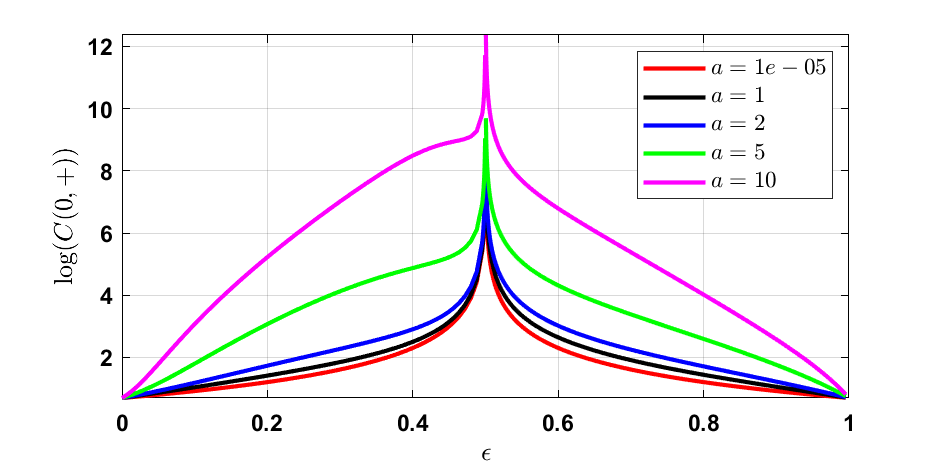
Figure 2: The conditional expectation of exit time $C(0,+)$ for a particle starting at the origin in an internal positive velocity state, for a drift alternating between $\mu=1/2$ on $[0,a(1-\epsilon)[$ and $-\mu$ on $[a(1-\epsilon),a[$, as a function of $\epsilon$.

5 Discussion and outlook

We have obtained a closed-form expression for the probability of exit and mean first- passage time at the origin of a run-and-tumble particle in any periodic force field whose values allow the particle to access any position on the positive real line. The particle is found to exit the system in finite time with probability $1$ if and only if the force field satisfies a condition expressed an an integral over its period.

We have calculated the average of the first-passage time at the origin, over the trajectories that exit the system in finite time. Periodicity has been used to obtain one of the boundary conditions. The results generalize the ones obtained in the presence of a constant subcritical drift. In particular, the mean exit time of a particle starting at the origin in positive velocity is strictly positive, and becomes large at the separation between the two regimes of almost-sure exit and non-zero survival probability, just as in the case of a constant drift. As noted in [23] in the case of almost-sure exit, the higher moments of the exit time can in principle be calculated iteratively, based on the Taylor expansion of the Laplace transform of the flow of particles through the origin.

The calculations become more tedious in the case of non-zero survival probability, however we can interpret the quantity $J(a)$ in a self-consistent way, in the limit where the period $a$ is short compared to the mean free path of the particle. Let us assume that the mean free path of the particle is large compared to $a$. It can be approximated by $N_{\pm}a$, where the neglected length in in $[-a,a]$ (during which the internal velocity state is $\pm v$). Moreover, let us look for an effective drift $\mu_{\mathrm{eff}}$ such that the length of a typical run is $\mu_{\mathrm{eff}}\pm v$ (depending on the internal velocity state of the particle). Integrating the equations of motion (Eqs (4,5)), we can approximate the duration of the average run $t_{\pm}$ in each of the two internal velocity states:

$$\begin{split}N_{\pm}a(\mu_{\mathrm{eff}}\pm v)^{-1}=\int_{0}^{N_{\pm}a}\frac{dx}{F(x)+v}.\end{split}$$ (108)

Dividing both sides by $N_{+}$ (resp. $N_{-}$) and using periodicity yields the system

$$a(\mu_{\mathrm{eff}}\pm v)^{-1}=\int_{0}^{N_{\pm}a}\frac{dx}{F(x)\pm v}.$$ (109)

The sum and difference of the above equations read

$$\begin{split}\frac{2a\mu_{\mathrm{eff}}}{v^{2}-\mu_{\mathrm{eff}}}=&\int_{0}^{a}\frac{2F(x)dx}{v^{2}-F(x)^{2}}\\ \frac{2av}{v^{2}-\mu_{\mathrm{eff}}}=&\int_{0}^{a}\frac{2vdx}{v^{2}-F(x)^{2}}.\end{split}$$ (110)

The effective drift $\mu_{\mathrm{eff}}$ follows as

$$\mu_{\mathrm{eff}}=\frac{v\int_{0}^{a}\frac{2F(x)dx}{v^{2}-F(x)^{2}}}{2\int_{0}^{a}\frac{2v}{v^{2}-F(x)^{2}}},$$ (111)

which has the same sign as the quantity $J(a)$. In the case of a fast-alternating force field, this effective drift coincide with the value identified in Eq. (61) in the limit of a short period interval $a$. The conditional mean first-passage time at the origin in this limit is $|\mu_{\mathrm{eff}}|^{-1}$, which generalizes the result obtained in [17] for a constant drift.

The model can be generalized in several ways. To make the model more realistic, one could take into account the nonzero duration of tumbles, and model the tumble time as an exponential random variable (in colonies of bacteria, tumble times and run times have the same order of magnitude [32]). Such a model has been solved in dimension $d$ for the survival probability of a run-and-tumble particle with an absorbing hyperplane and zero force field, if the particle starts on the hyperplane [33]. Quite remarkably, the result does not depend on the dimension.

One can consider models of RTPs with an absorbing hyperplane. This problem has been solved in presence of a constant drift in [17]. Technically, the evolution equation of the system becomes a coupled system of backward Fokker–Planck equations (one for every value of the projection of the internal velocity on the normal direction to the absorbing hyperplane).

Appendix A Evaluation of the functions $J$ and $\Xi_{\pm}$

Let $f$ be a periodic function of period $a$. The functions $J$ and $\Xi_{n}$ defined in Eqs (31,34) can be evaluated on the entire positive half line once the values are known on the interval $[0,a[$. Indeed, for $x$ in $[0,a[$ and a positive integer $N$:

$$\begin{split}J(x+Na)=&\sum_{k=0}^{N-1}\int_{ka}^{(k+1)a}dy\frac{2F(y)}{1-F(y)^{2}}+\int_{Na}^{x}dy\frac{2F(y)}{1-F(y)^{2}}\\ =&NJ(a)+J(x),\end{split}$$ (112)

Assuming $J(a)\neq 0$,

$$\begin{split}\Xi_{n}(x+Na)=&\left(\sum_{k=0}^{N-1}\int_{ka}^{(k+1)a}\frac{e^{nJ(x)}}{1-F(x)^{2}}dx\right)+\int_{Na}^{Na+x}\frac{e^{nJ(v)}}{1-F(v)^{2}}dv\\ =&\left(\sum_{k=0}^{N-1}e^{nkJ(a)}\Xi_{n}(a)\right)+e^{nNJ(a)}\Xi_{n}(x)\\ =&\frac{1-e^{nNJ(a)}}{1-e^{nJ(a)}}\Xi_{n}(a)+e^{nNJ(a)}\Xi_{n}(x),\\ &\qquad x\in[0,a],\qquad N\in\mathbb{N}^{\ast},\qquad n\in\{-1,+1\}.\end{split}$$ (113)

$$\begin{split}\int_{0}^{x+Na}\Xi^{\prime}_{m}(v)\Xi_{n}(v)dv=&\sum_{k=0}^{N-1}\int_{ka}^{(k+1)a}\Xi^{\prime}_{m}(v)\Xi_{n}(v)dv+\int_{Na}^{x+Na}\Xi^{\prime}_{m}(v)\Xi_{n}(v)dv\\ =&\sum_{k=0}^{N-1}\int_{0}^{a}\Xi^{\prime}_{m}(ka+v)\Xi_{n}(ka+v)dv+\int_{0}^{x}\Xi^{\prime}_{m}(Na+v)\Xi_{n}(Na+v)dv.\end{split}$$ (114)

By periodicity of the force field, $\Xi^{\prime}_{m}(ka+v)=e^{mJ(a)}\Xi^{\prime}_{m}(v)$, on the other hand $\Xi_{n}(ka+v)$ has been expressed in Eq. (113). Substituting yields

$$\begin{split}\int_{0}^{x+Na}\Xi^{\prime}_{m}(v)\Xi_{n}(v)dv=&\sum_{k=0}^{N-1}e^{mkJ(a)}\int_{0}^{a}\Xi^{\prime}_{m}(v)\Xi_{n}(ka+v)dv+e^{mNJ(a)}\int_{0}^{x}\Xi^{\prime}_{m}(v)\Xi_{n}(Na+v)dv\\ =&\sum_{k=0}^{N-1}e^{mkJ(a)}\int_{0}^{a}\Xi^{\prime}_{m}(v)\left[\frac{1-e^{nkJ(a)}}{1-e^{nJ(a)}}\Xi_{n}(a)+e^{nkJ(a)}\Xi_{m}(v)\right]dv\\ &+e^{mNJ(a)}\int_{0}^{x}\Xi^{\prime}_{m}(v)\left[\frac{1-e^{nNJ(a)}}{1-e^{nJ(a)}}\Xi_{n}(a)+e^{nNJ(a)}\Xi_{n}(v)\right]dv\\ =&\Xi_{m}(a)\Xi_{n}(a)\sum_{k=0}^{N-1}\frac{e^{mkJ(a)}(1-e^{nkJ(a)})}{1-e^{nJ(a)}}+\Xi_{m}(x)\Xi_{n}(a)e^{mNJ(a)}\frac{1-e^{nNJ(a)}}{1-e^{nJ(a)}}\\ +&\sum_{k=0}^{N-1}e^{(m+n)kJ(a)}\int_{0}^{a}\Xi^{\prime}_{m}(v)\Xi_{n}(v)dv+e^{(m+n)NJ(a)}\int_{0}^{x}\Xi^{\prime}_{m}(v)\Xi_{n}(v)dv.\\ \end{split}$$ (115)

In particular,

$$\begin{split}\int_{0}^{x+Na}\Xi^{\prime}_{-}(v)\Xi_{+}(v)dv=&\frac{\Xi_{-}(a)\Xi_{+}(a)}{1-e^{J(a)}}\left(-N+\frac{1-e^{-NJ(a)}}{1-e^{-J(a)}}\right)\\ +&\Xi_{-}(x)\Xi_{+}(a)e^{-NJ(a)}\frac{1-e^{NJ(a)}}{1-e^{J(a)}}\\ +&N\int_{0}^{a}\Xi^{\prime}_{-}(v)\Xi_{+}(v)dv+\int_{0}^{x}\Xi^{\prime}_{-}(v)\Xi_{+}(v)dv,\\ =&N\left[\int_{0}^{a}\Xi^{\prime}_{-}(v)\Xi_{+}(v)dv-\frac{\Xi_{-}(a)\Xi_{+}(a)}{1-e^{J(a)}}\right]\\ &+\frac{\Xi_{+}(a)}{1-e^{J(a)}}\left(\frac{\Xi_{-}(a)}{1-e^{-J(a)}}+\Xi_{-}(x)\right)+\int_{0}^{x}\Xi_{-}(v)\Xi_{+}(v)dv\\ &-\frac{\Xi_{+}(a)e^{-NJ(a)}}{1-e^{J(a)}}\left(\frac{\Xi_{-}(a)}{1-e^{-J(a)}}+\Xi_{-}(x)\right),\end{split}$$ (116)

where we have collected the terms of order $N$, $1$ and $e^{-NJ(a)}$. Moreover,

$$\begin{split}\int_{0}^{x+Na}\Xi^{\prime}_{+}(v)\Xi_{-}(v)dv=&\frac{\Xi_{+}(a)\Xi_{-}(a)}{1-e^{-J(a)}}\left(-N+\frac{1-e^{+NJ(a)}}{1-e^{+J(a)}}\right)\\ +&\Xi_{+}(x)\Xi_{-}(a)e^{+NJ(a)}\frac{1-e^{-NJ(a)}}{1-e^{-J(a)}}\\ +&N\int_{0}^{a}\Xi^{\prime}_{+}(v)\Xi_{-}(v)dv+\int_{0}^{x}\Xi^{\prime}_{+}(v)\Xi_{-}(v)dv\\ =&\frac{\Xi_{-}(a)e^{NJ(a)}}{1-e^{-J(a)}}\left(-\frac{\Xi_{+}(a)}{1-e^{J(a)}}+\Xi_{+}(x)\right)\\ &+N\left[\int_{0}^{a}\Xi^{\prime}_{+}(v)\Xi_{-}(v)dv-\frac{\Xi_{-}(a)\Xi_{+}(a)}{1-e^{-J(a)}}\right]\\ &+\frac{\Xi_{-}(a)}{1-e^{-J(a)}}\left(\frac{\Xi_{+}(a)}{1-e^{J(a)}}+\Xi_{+}(x)\right)+\int_{0}^{x}\Xi^{\prime}_{+}(v)\Xi_{-}(v)dv,\\ \end{split}$$ (117)

where we have collected the terms of order $e^{NJ(a)}$, $N$, and $1$.

Appendix B Evaluation of the functions $\varphi$ and $\psi$

Consider a nonnegative integer $N$, ad $x$ in $[0,a[$. To express the function $t$ at $x+Na$, we need to evaluate the integral

$$\varphi(Na+x)=e^{-J(x+Na)}\left(\sum_{k=0}^{N-1}\int_{ka}^{(k+1)a}dy\frac{e(y)F(y)-E(y)}{1-F(y)^{2}}e^{J(y)}+\int_{Na}^{Na+x}dy\frac{e(y)F(y)-E(y)}{1-F(y)^{2}}e^{J(y)}\right)$$ (118)

Let us assume $J(a)>0$. In this case,

$$\begin{split}e(y)=&e(0)\exp(-J(y)),\\ E(y)=&E(0)+2e(0)\Xi_{-}(y).\\ \end{split}$$ (119)

with $e(0)<0$ as in Eq. (43). As $f$ is $a$-periodic,

$$\begin{split}\varphi&(Na+x)=\\ &e^{-NJ(a)-J(x)}\left[\sum_{k=0}^{N-1}\int_{0}^{a}dy\left(\frac{F(y)}{1-F(y)^{2}}-\frac{E(0)+2e(0)\left[\frac{1-e^{-kJ(a)}}{1-e^{-J(a)}}\Xi_{-}(a)+e^{-kJ(a)}\Xi_{-}(y)\right]}{1-F(y)^{2}}e^{kJ(a)+J(y)}\right)\right.\\ &\left.+\int_{0}^{x}dy\left(\frac{F(y)}{1-F(y)^{2}}-\frac{E(0)+2e(0)\left[\frac{1-e^{-NJ(a)}}{1-e^{-J(a)}}\Xi_{-}(a)+e^{-NJ(a)}\Xi_{-}(y)\right]}{1-F(y)^{2}}e^{NJ(a)+J(y)}\right)\right]\\ =&e^{-NJ(a)-J(x)}\times N\left[\int_{0}^{a}dy\frac{F(y)}{1-F(y)^{2}}+\frac{2e(0)\Xi_{-}(a)}{1-e^{-J(a)}}\int_{0}^{a}dy\frac{e^{J(y)}}{1-F(y)^{2}}-2e(0)\int_{0}^{a}dy\frac{e^{J(y)}\Xi_{-}(y)}{1-F(y)^{2}}\right]\\ &-e^{-NJ(a)-J(x)}\times\int_{0}^{a}dy\left(E(0)+\frac{2e(0)}{1-e^{-J(a)}}\right)\frac{1-e^{NJ(a)}}{(1-F(y)^{2})(1-e^{J(a)})}e^{J(y)}\\ &+e^{-NJ(a)-J(x)}\left[\int_{0}^{x}dy\frac{F(y)}{1-F(y)^{2}}-\left(E(0)+2e(0)\frac{1-e^{-NJ(a)}}{1-e^{-J(a)}}\right)e^{NJ(a)}\int_{0}^{x}dy\frac{e^{J(y)}}{1-F(y)^{2}}\right.\\ &\left.-2e(0)\int_{0}^{x}dy\frac{e^{J(y)}\Xi_{-}(y)}{1-F(y)^{2}}\right].\end{split}$$ (120)

Let us reorganize the above expression by grouping the terms according to their dependence on $N$. The dominant term is of order $1$ in the large-$N$ limit:

$$\begin{split}\varphi(Na+x)=&\left[\frac{1}{(1-e^{J(a)})}\times\left(E(0)+\frac{2e(0)}{1-e^{-J(a)}}\right)\int_{0}^{a}dy\frac{e^{J(y)}}{(1-F(y)^{2})}\right]e^{-J(x)}\\ &-\left(E(0)+\frac{2e(0)}{1-e^{-J(a)}}\right)e^{-J(x)}\int_{0}^{x}\frac{e^{J(y)}}{1-F(y)^{2}}\\ &e^{-NJ(a)}e^{-J(x)}\times N\left[\int_{0}^{a}dy\frac{F(y)}{1-F(y)^{2}}+\frac{2e(0)\Xi_{-}(a)}{1-e^{-J(a)}}\int_{0}^{a}dy\frac{e^{J(y)}}{1-F(y)^{2}}-2e(0)\int_{0}^{a}dy\frac{e^{J(y)}\Xi_{-}(y)}{1-F(y)^{2}}\right]\\ &+e^{-NJ(a)}\left[-e^{-J(x)}\int_{0}^{a}\left(E(0)+\frac{2e(0)}{1-e^{-J(a)}}\right)\frac{1}{(1-F(y)^{2})(1-e^{J(a)})}e^{J(y)}\right.\\ &+\left.e^{-J(x)}\int_{0}^{x}dy\frac{F(y)-2e(0)e^{J(y)}\Xi_{-}(y)}{1-F(y)^{2}}\right]\\ =:&C_{1}e^{-J(x)}+C_{2}e^{-J(x)}\Xi_{-}(x)\\ &+C_{3}Ne^{-NJ(a)}e^{-J(x)}\\ &+e^{-NJ(a)}\left[C_{4}e^{-J(x)}+C_{5}e^{-J(x)}\int_{0}^{x}dy\frac{F(y)-2e(0)e^{J(y)}\Xi_{-}(y)}{1-F(y)^{2}}\right].\end{split}$$ (121)

We need to evaluate the following integral which the first term in the expression on $\psi(x+Na)$:

$$\begin{split}\int_{0}^{x+Na}dy\frac{\varphi(y)}{1-F(y)^{2}}=&\sum_{k=0}^{N-1}\int_{0}^{a}dy\frac{\varphi(ka+y)}{1-F(y)^{2}}+\int_{0}^{x}dy\frac{\varphi(Na+y)}{1-F(y)^{2}}\\ =&\sum_{k=0}^{N-1}\mathcal{I}_{k}(a)+\mathcal{I}_{N}(x),\\ \end{split}$$ (122)

with $\mathcal{I}_{N}(x)$ defined for any nonnegative integer $N$ and any $x$ in $[0,a]$ as:

$$\begin{split}\mathcal{I}_{N}(x)=&\int_{0}^{x}dy\frac{1}{1-F(y)^{2}}\left[C_{1}e^{-J(Na+y)}+C_{2}e^{-J(Na+y)}\Xi_{-}(Na+y)\right.\\ &+C_{3}Ne^{-NJ(a)}e^{-J(Na+y)}\\ &\left.+e^{-NJ(a)}\left(C_{4}e^{-J(Na+y)}+C_{5}e^{-J(Na+y)}\int_{0}^{Na+y}dz\frac{F(z)-2e(0)e^{J(z)}\Xi_{-}(z)}{1-F(z)^{2}}\right)\right]\\ =&C_{1}e^{-NJ(a)}\Xi_{-}(x)\\ &+C_{2}\left[e^{-NJ(a)}\frac{1-e^{-NJ(a)}}{1-e^{-J(a)}}\Xi_{-}(a)\Xi_{-}(x)+e^{-2NJ(a)}\int_{0}^{x}dy\frac{\Xi_{-}(y)}{1-F(y)^{2}}\right]\\ &+C_{3}Ne^{-2NJ(a)}\Xi_{-}(x)\\ &+C_{4}e^{-2NJ(a)}\Xi_{-}(x)\\ &+C_{5}e^{-NJ(a)}\int_{0}^{x}dy\frac{e^{-J(y)}}{1-F(y)^{2}}\int_{0}^{Na+y}dz\left[\frac{F(z)}{1-F(z)^{2}}-2e(0)\frac{e^{J(z)}\Xi_{-}(z)}{1-F(z)^{2}}\right].\end{split}$$ (123)

The terms proportional to $C_{5}$ can be evaluated using periodicity and integration by parts:

$$\begin{split}\int_{0}^{x}dy&\frac{e^{-J(y)}}{1-F(y)^{2}}\int_{0}^{Na+y}dz\left[\frac{F(z)}{1-F(z)^{2}}-2e(0)\frac{e^{J(z)}\Xi_{-}(z)}{1-F(z)^{2}}\right]\\ =&\Xi_{-}(x)\int_{0}^{Na+x}dz\left[\frac{F(z)}{1-F(z)^{2}}-2e(0)\frac{e^{J(z)}\Xi_{-}(z)}{1-F(z)^{2}}\right]\\ &-\int_{0}^{x}dy\Xi_{-}(y)\left[\frac{F(Na+y)}{1-F(Na+y)^{2}}-2e(0)\frac{e^{J(Na+y)}\Xi_{-}(Na+y)}{1-F(Na+y)^{2}}\right]\\ =&\Xi_{-}(x)\left[N\int_{0}^{a}dz\frac{F(z)}{1-F(z)^{2}}+\int_{0}^{x}dz\frac{F(z)}{1-F(z)^{2}}\right.\\ &\left.-2e(0)\sum_{k=0}^{N-1}e^{kJ(a)}\int_{0}^{a}dz\frac{e^{J(z)}\Xi_{-}(ka+z)}{1-F(z)^{2}}-2e(0)e^{NJ(a)}\int_{0}^{x}dz\frac{e^{J(z)}\Xi_{-}(Na+z)}{1-F(z)^{2}}dz\right]\\ &-\int_{0}^{x}dy\frac{\Xi_{-}(y)F(y)}{1-F(y)^{2}}+2e(0)e^{NJ(a)}\int_{0}^{x}dy\frac{e^{J(y)}\Xi_{-}(y)\Xi_{-}(Na+y)}{1-F(y)^{2}}\\ =&\Xi_{-}(x)\left[N\int_{0}^{a}dz\frac{F(z)}{1-F(z)^{2}}+\int_{0}^{x}dz\frac{F(z)}{1-F(z)^{2}}\right.\\ &\left.-2e(0)\sum_{k=0}^{N-1}e^{kJ(a)}\int_{0}^{a}dz\frac{e^{J(z)}}{1-F(z)^{2}}\left(\frac{1-e^{-kJ(a)}}{1-e^{-J(a)}}\Xi_{-}(a)+e^{-kJ(a)}\Xi_{-}(z)\right)\right.\\ &\left.-2e(0)e^{NJ(a)}\int_{0}^{x}dz\frac{e^{J(z)}}{1-F(z)^{2}}dz\left(\frac{1-e^{-NJ(a)}}{1-e^{-J(a)}}\Xi_{-}(a)+e^{-NJ(a)}\Xi_{-}(z)\right)\right]\\ &-\int_{0}^{x}dy\frac{\Xi_{-}(y)F(y)}{1-F(y)^{2}}+2e(0)e^{NJ(a)}\int_{0}^{x}dy\frac{e^{J(y)}\Xi_{-}(y)}{1-F(y)^{2}}\left(\frac{1-e^{-NJ(a)}}{1-e^{-J(a)}}\Xi_{-}(a)+e^{-NJ(a)}\Xi_{-}(y)\right)\\ =&\Xi_{-}(x)\left[N\int_{0}^{a}dz\frac{F(z)}{1-F(z)^{2}}+\int_{0}^{x}dz\frac{F(z)}{1-F(z)^{2}}\right.\\ &\left.-2e(0)\frac{\Xi_{-}(a)\Xi_{+}(a)}{1-e^{-J(a)}}\left(-N+\frac{1-e^{NJ(a)}}{1-e^{J(a)}}\right)-2Ne(0)\int_{0}^{a}dz\Xi^{\prime}_{+}(z)\Xi_{-}(z)\right.\\ &\left.-2e(0)\frac{e^{NJ(a)}-1}{1-e^{-J(a)}}\Xi_{+}(x)-2e(0)\int_{0}^{x}dz\Xi^{\prime}_{+}(z)\Xi_{-}(z)\right]\\ &-\int_{0}^{x}dy\frac{\Xi_{-}(y)F(y)}{1-F(y)^{2}}+2e(0)\Xi_{-}(a)\frac{e^{NJ(a)}-1}{1-e^{-J(a)}}\int_{0}^{x}dy\Xi^{\prime}_{+}(y)\Xi_{-}(y)+2e(0)\int_{0}^{x}dy\Xi^{\prime}_{+}(y)\left(\Xi_{-}(y)\right)^{2},\\ \end{split}$$ (124)

where we used the expression of $\Xi_{-}(ka+x)$ given in Eq. (113) and worked out geometric sums.

Rearranging terms according to their dependence on $N$ yields:

$$\begin{split}\int_{0}^{x}dy&\frac{e^{-J(y)}}{1-F(y)^{2}}\int_{0}^{Na+y}dz\left[\frac{F(z)}{1-F(z)^{2}}-2e(0)\frac{e^{J(z)}\Xi_{-}(z)}{1-F(z)^{2}}\right]\\ =&L(x)e^{NJ(a)}+M(x)N+U(x),\end{split}$$ (125)

with

$$\begin{split}L(x):=&2e(0)\frac{1}{1-e^{-J(a)}}\left[\frac{\Xi_{-}(a)\Xi_{+}(a)\Xi_{-}(x)}{1-e^{J(a)}}-\frac{1}{1-e^{-J(a)}}\Xi_{+}(x)^{2}-\Xi_{-}(a)\int_{0}^{x}dy\Xi^{\prime}_{+}(y)\Xi_{-}(y)\right],\\ M(x):=&\Xi_{-}(x)\int_{0}^{a}dz\frac{F(z)}{1-F(z)^{2}}+2e(0)\frac{\Xi_{-}(a)\Xi_{+}(a)\Xi_{-}(x)}{1-e^{J(a)}}-2e(0)\Xi_{-}(x)\int_{0}^{a}dy\Xi^{\prime}_{+}(y)\Xi_{-}(y),\\ U(x):=&\Xi_{-}(x)\left[\int_{0}^{x}dz\frac{F(z)}{1-F(z)^{2}}-2e(0)\frac{\Xi_{-}(a)\Xi_{+}(a)}{1-e^{-J(a)}}\left(+\frac{1}{1-e^{J(a)}}\right)\right.\\ &\left.+2e(0)\frac{1}{1-e^{-J(a)}}\Xi_{+}(x)-2e(0)\int_{0}^{x}dz\Xi^{\prime}_{+}(z)\Xi_{-}(z)\right]\\ &-\int_{0}^{x}dy\frac{\Xi_{-}(y)F(y)}{1-F(y)^{2}}-2e(0)\Xi_{-}(a)\frac{1}{1-e^{-J(a)}}\int_{0}^{x}dy\Xi^{\prime}_{+}(y)\Xi_{-}(y)+2e(0)\int_{0}^{x}dy\Xi^{\prime}_{+}(y)\left(\Xi_{-}(y)\right)^{2}.\\ \end{split}$$ (126)

Grouping the terms in the expression of $\mathcal{I}_{N}(x)$ according to their dependence on $N$ now yields:

$$\begin{split}\mathcal{I}_{N}(x)=&C_{5}L(x)\\ &+C_{5}M(x)Ne^{-NJ(a)}\\ &+C_{3}\Xi_{-}(x)Ne^{-2NJ(a)}\\ &+\left[C_{1}\Xi_{-}(x)+C_{2}\frac{\Xi_{-}(a)\Xi_{-}(x)}{1-e^{-J(a)}}+C_{5}U(x)\right]e^{-NJ(a)}\\ &+\left[-C_{2}\frac{\Xi_{-}(a)\Xi_{-}(x)}{1-e^{-J(a)}}+C_{2}\int_{0}^{x}dy\frac{\Xi_{-}(y)}{1-F(y)^{2}}+C_{4}\Xi_{-}(x)\right]e^{-2NJ(a)}\\ =:&\tau_{1}(x)+\tau_{2}(x)Ne^{-NJ(a)}+\tau_{3}(x)Ne^{-2NJ(a)}+\tau_{4}(x)e^{-NJ(a)}+\tau_{5}(x)e^{-2NJ(a)}.\\ \end{split}$$ (127)

The leading term at large $N$ in the sum of Eq. (122) is therefore $C_{5}L(x)N$. The sums in Eq. (122) can be calculated exactly, using the identity

$$\begin{split}\sum_{k=0}^{N-1}kx^{k}&=x\frac{d}{dx}\left(\sum_{k=0}^{N-1}x^{k}\right)\\ =&x\frac{d}{dx}\left(\frac{1-x^{N}}{1-x}\right)\\ =&\frac{x(1-x^{N})}{(1-x)^{2}}-N\frac{x^{N}}{1-x}=\frac{(N-1)^{N+1}-Nx^{N}+x}{(1-x)^{2}}.\end{split}$$ (128)

From Eqs (122,127), we obtain

$$\begin{split}\int_{0}^{x+Na}dy\frac{\varphi(y)}{1-F(y)^{2}}=&\sum_{k=0}^{N-1}\mathcal{I}_{k}(a)+\mathcal{I}_{N}(x)\\ =&N\tau_{1}(a)\\ &+\frac{(N-1)e^{-(N+1)J(a)}-Ne^{-NJ(a)}+e^{-J(a)}}{(1-e^{-J(a)})^{2}}\tau_{2}(x)\\ &+\frac{(N-1)e^{-2(N+1)J(a)}-Ne^{-2NJ(a)}+e^{-2J(a)}}{(1-e^{-2J(a)})^{2}}\tau_{3}(x)\\ &+\frac{1-e^{-NJ(a)}}{1-e^{-J(a)}}\tau_{4}(x)+\frac{1-e^{-2NJ(a)}}{1-e^{-2J(a)}}\tau_{5}(x)\\ &+\tau_{1}(x)+\tau_{2}(x)Ne^{-NJ(a)}+\tau_{3}(x)Ne^{-2NJ(a)}+\tau_{4}(x)e^{-NJ(a)}+\tau_{5}(x)e^{-2NJ(a)}\\ =&N\tau_{1}(a)\\ &+\frac{e^{-J(a)}}{(1-e^{J(a)})^{2}}\tau_{2}(x)+\frac{e^{-2J(a)}}{(1-e^{-2J(a)})^{2}}\tau_{3}(x)+\frac{1}{1-e^{-J(a)}}\tau_{4}(x)+\frac{1}{1-e^{-2J(a)}}\tau_{5}(x)\\ &-\frac{e^{-J(a)}}{1-e^{-J(a)}}\tau_{2}(x)Ne^{-NJ(a)}-\frac{e^{-2J(a)}}{1-e^{-2J(a)}}\tau_{3}(x)Ne^{-2NJ(a)}\\ &-\frac{e^{-J(a)}}{(1-e^{-J(a)})^{2}}\tau_{2}(x)e^{-NJ(a)}\\ &+\left(1-\frac{1}{1-e^{-J(a)}}\right)\tau_{4}(x)e^{-NJ(a)}\\ &+\left(1-\frac{1}{1-e^{-2J(a)}}\right)\tau_{2}(x)e^{-2NJ(a)}.\end{split}$$ (129)

The following integral in the expression $\psi(x+Na)$ is evaluated by taking similar calculational steps:

$$\begin{split}\int_{0}^{Na+x}dy&\frac{E(y)F(y)-e(y)}{1-F(y)^{2}}=\\ &\sum_{k=0}^{N-1}\int_{ka}^{(k+1)a}dy\frac{E(y)F(y)-e(y)}{1-F(y)^{2}}+\int_{Na}^{Na+x}dy\frac{E(y)F(y)-e(y)}{1-F(y)^{2}}\\ =&\sum_{k=0}^{N-1}\int_{0}^{a}dy\frac{[E(0)+2e(0)\Xi_{-}(ka+y)]F(y)-e(0)\exp(-J(ka+y))}{1-F(y)^{2}}\\ &+\int_{0}^{x}dy\frac{[E(0)+2e(0)\Xi_{-}(Na+y)]F(y)-e(0)\exp(-J(Na+y))}{1-F(y)^{2}}\\ =&\sum_{k=0}^{N-1}\int_{0}^{a}dy\frac{[E(0)+2e(0)\left(\frac{1-e^{-kJ(a)}}{1-e^{-J(a)}}\Xi_{-}(a)+e^{-kJ(a)}\Xi_{-}(x)\right)]F(y)-e(0)e^{-kJ(a)}e^{-J(y)}}{1-F(y)^{2}}\\ &+\int_{0}^{x}dy\frac{[E(0)+2e(0)\left(\frac{1-e^{-NJ(a)}}{1-e^{-J(a)}}\Xi_{-}(a)+e^{-NJ(a)}\Xi_{-}(x)\right)]F(y)-e(0)e^{-NJ(a)}e^{-J(y)}}{1-F(y)^{2}}\\ =&N\int_{0}^{a}dy\left(E(0)+\frac{2e(0)}{1-e^{-J(a)}}\Xi_{-}(a)\right)\frac{1}{1-F(y)^{2}}\\ &+\frac{1-e^{-NJ(a)}}{1-e^{-J(a)}}\left[-\frac{2e(0)\Xi_{-}(a)}{1-e^{-J(a)}}\int_{0}^{a}\frac{dy}{1-F(y)^{2}}\right.\\ &\left.+2e(0)\int_{0}^{a}dy\frac{\Xi_{-}(y)}{1-F(y)^{2}}-e(0)\int_{0}^{a}dy\frac{e^{-J(y)}}{1-F(y)^{2}}\right]\\ &+\int_{0}^{x}dy\left(E(0)+\frac{2e(0)}{1-e^{-J(a)}}\Xi_{-}(a)\right)\frac{1}{1-F(y)^{2}}\\ &+e^{-NJ(a)}\left[-\frac{2e(0)\Xi_{-}(a)}{1-e^{-J(a)}}\int_{0}^{a}\frac{dy}{1-F(y)^{2}}\right.\\ &\left.+2e(0)\int_{0}^{a}dy\frac{\Xi_{-}(y)}{1-F(y)^{2}}-e(0)\int_{0}^{a}dy\frac{e^{-J(y)}}{1-F(y)^{2}}\right].\\ \end{split}$$ (130)

From the value of $e(0)$ obtained in Eq. (43) in the case $J(a)>0$, and the boundary condition $E(0)=e(0)+1$, the coefficient of $N$ vanishes in the above expression. Indeed:

$$\begin{split}E(0)+\frac{2e(0)}{1-e^{-J(a)}}\Xi_{-}(a)=&e(0)\frac{1-e^{-J(a)}+2\Xi_{-}(a)}{1-e^{-J(a)}}+1\\ =&-1+1=0.\end{split}$$ (131)

Grouping the remaining terms according to their large-$N$ behavior yields

$$\begin{split}\int_{0}^{Na+x}dy&\frac{E(y)F(y)-e(y)}{1-F(y)^{2}}=\\ =&N\int_{0}^{a}dy\left(E(0)+\frac{2e(0)}{1-e^{-J(a)}}\Xi_{-}(a)\right)\frac{1}{1-F(y)^{2}}\\ &+\frac{1}{1-e^{-J(a)}}\left[-\frac{2e(0)\Xi_{-}(a)}{1-e^{-J(a)}}\int_{0}^{a}\frac{dy}{1-F(y)^{2}}\right.\\ &\left.+2e(0)\int_{0}^{a}dy\frac{\Xi_{-}(y)}{1-F(y)^{2}}-e(0)\int_{0}^{a}dy\frac{e^{-J(y)}}{1-F(y)^{2}}\right]\\ &+\left.\int_{0}^{x}dy\left(E(0)+\frac{2e(0)}{1-e^{-J(a)}}\Xi_{-}(a)\right)\frac{1}{1-F(y)^{2}}\right.\\ &+e^{-NJ(a)}\left[-\frac{1}{1-e^{-J(a)}}\left[-\frac{2e(0)\Xi_{-}(a)}{1-e^{-J(a)}}\int_{0}^{a}\frac{dy}{1-F(y)^{2}}\right.\right.\\ &\left.+2e(0)\int_{0}^{a}dy\frac{\Xi_{-}(y)}{1-F(y)^{2}}-e(0)\int_{0}^{a}dy\frac{e^{-J(y)}}{1-F(y)^{2}}\right]\\ &\left.-\frac{2e(0)\Xi_{-}(a)}{1-e^{-J(a)}}\int_{0}^{a}\frac{dy}{1-F(y)^{2}}+2e(0)\int_{0}^{a}dy\frac{\Xi_{-}(y)}{1-F(y)^{2}}-e(0)\int_{0}^{a}dy\frac{e^{-J(y)}}{1-F(y)^{2}}\right].\\ \end{split}$$ (132)

References

- [1] S. Redner, A guide to first-passage processes. Cambridge university press, 2001.
- [2] P. Patie, On some first passage time problems motivated by financial applications. PhD thesis, Universität Zürich, 2004.
- [3] A. E. Kyprianou, Introductory lectures on fluctuations of Lévy processes with applications. Springer Science & Business Media, 2006.
- [4] X. Duhalde, C. Foucart, and C. Ma, “On the hitting times of continuous-state branching processes with immigration,” Stochastic Processes and their Applications, vol. 124, no. 12, pp. 4182–4201, 2014.
- [5] C. Foucart and M. Vidmar, “Continuous-state branching processes with collisions: first passage times and duality,” Stochastic Processes and their Applications, vol. 167, p. 104230, 2024.
- [6] H. C. Berg and D. A. Brown, “Chemotaxis in escherichia coli analysed by three-dimensional tracking,” Nature, vol. 239, no. 5374, pp. 500–504, 1972.
- [7] H. C. Berg, E. coli in Motion. Springer Science & Business Media, 2008.
- [8] S. Ramaswamy, “The mechanics and statistics of active matter,” 2010.
- [9] M. E. Cates and J. Tailleur, “Motility-induced phase separation,” Annu. Rev. Condens. Matter Phys., vol. 6, no. 1, pp. 219–244, 2015.
- [10] H. G. Othmer, S. R. Dunbar, and W. Alt, “Models of dispersal in biological systems,” Journal of mathematical biology, vol. 26, no. 3, pp. 263–298, 1988.
- [11] K. Martens, L. Angelani, R. Di Leonardo, and L. Bocquet, “Probability distributions for the run-and-tumble bacterial dynamics: An analogy to the lorentz model,” The European Physical Journal E, vol. 35, pp. 1–6, 2012.
- [12] G. H. Weiss, “Some applications of persistent random walks and the telegrapher’s equation,” Physica A: Statistical Mechanics and its Applications, vol. 311, no. 3-4, pp. 381–410, 2002.
- [13] I. Santra, U. Basu, and S. Sabhapandit, “Run-and-tumble particles in two dimensions: Marginal position distributions,” Phys. Rev. E, vol. 101, p. 062120, Jun 2020.
- [14] P. Le Doussal, S. N. Majumdar, and G. Schehr, “Noncrossing run-and-tumble particles on a line,” Physical Review E, vol. 100, no. 1, p. 012113, 2019.
- [15] M. R. Evans and S. N. Majumdar, “Run and tumble particle under resetting: a renewal approach,” Journal of Physics A: Mathematical and Theoretical, vol. 51, no. 47, p. 475003, 2018.
- [16] I. Santra, U. Basu, and S. Sabhapandit, “Run-and-tumble particles in two dimensions under stochastic resetting conditions,” Journal of Statistical Mechanics: Theory and Experiment, vol. 2020, p. 113206, nov 2020.
- [17] B. De Bruyne, S. N. Majumdar, and G. Schehr, “Survival probability of a run-and-tumble particle in the presence of a drift,” Journal of Statistical Mechanics: Theory and Experiment, vol. 2021, no. 4, p. 043211, 2021.
- [18] P. Singh, S. Sabhapandit, and A. Kundu, “Run-and-tumble particle in inhomogeneous media in one dimension,” Journal of Statistical Mechanics: Theory and Experiment, vol. 2020, no. 8, p. 083207, 2020.
- [19] P. Singh, S. Santra, and A. Kundu, “Extremal statistics of a one-dimensional run and tumble particle with an absorbing wall,” Journal of Physics A: Mathematical and Theoretical, vol. 55, no. 46, p. 465004, 2022.
- [20] L. Angelani, “One-dimensional run-and-tumble motions with generic boundary conditions,” Journal of Physics A: Mathematical and Theoretical, vol. 56, no. 45, p. 455003, 2023.
- [21] K. Malakar, V. Jemseena, A. Kundu, K. V. Kumar, S. Sabhapandit, S. N. Majumdar, S. Redner, and A. Dhar, “Steady state, relaxation and first-passage properties of a run-and-tumble particle in one-dimension,” Journal of Statistical Mechanics: Theory and Experiment, vol. 2018, no. 4, p. 043215, 2018.
- [22] M. Guéneau, S. N. Majumdar, and G. Schehr, “Optimal mean first-passage time of a run-and-tumble particle in a class of one-dimensional confining potentials,” Europhysics Letters, vol. 145, no. 6, p. 61002, 2024.
- [23] M. Guéneau, S. N. Majumdar, and G. Schehr, “Run-and-tumble particle in one-dimensional potentials: mean first-passage time and applications,” arXiv preprint arXiv:2409.16951, 2024.
- [24] M. Guéneau and L. Touzo, “Relating absorbing and hard wall boundary conditions for a one-dimensional run-and-tumble particle,” Journal of Physics A: Mathematical and Theoretical, vol. 57, no. 22, p. 225005, 2024.
- [25] P. Le Doussal, S. N. Majumdar, and G. Schehr, “Velocity and diffusion constant of an active particle in a one-dimensional force field,” Europhysics Letters, vol. 130, no. 4, p. 40002, 2020.
- [26] S. K. Nath and S. Sabhapandit, “Survival probability and position distribution of a run and tumble particle in potential with an absorbing boundary,” arXiv preprint arXiv:2405.18988, 2024.
- [27] P. C. Bressloff, “Encounter-based model of a run-and-tumble particle ii: absorption at sticky boundaries,” Journal of Statistical Mechanics: Theory and Experiment, vol. 2023, no. 4, p. 043208, 2023.
- [28] C. Roberts and Z. Zhen, “Run-and-tumble motion in a linear ratchet potential: Analytic solution, power extraction, and first-passage properties,” Physical Review E, vol. 108, no. 1, p. 014139, 2023.
- [29] A. J. Bray, S. N. Majumdar, and G. Schehr, “Persistence and first-passage properties in nonequilibrium systems,” Advances in Physics, vol. 62, no. 3, pp. 225–361, 2013.
- [30] A. Dhar, A. Kundu, S. N. Majumdar, S. Sabhapandit, and G. Schehr, “Run-and-tumble particle in one-dimensional confining potentials: Steady-state, relaxation, and first-passage properties,” Physical Review E, vol. 99, no. 3, p. 032132, 2019.
- [31] J. R. Norris, Markov chains. No. 2, Cambridge university press, 1998.
- [32] H. C. Berg, E. coli in Motion. Springer, 2004.
- [33] F. Mori, P. Le Doussal, S. N. Majumdar, and G. Schehr, “Universal survival probability for a d-dimensional run-and-tumble particle,” Physical review letters, vol. 124, no. 9, p. 090603, 2020.