A Linear Differential Inclusion for Contraction Analysis to Known Trajectories

Abstract

Infinitesimal contraction analysis provides exponential convergence rates between arbitrary pairs of trajectories of a system by studying the system’s linearization. An essentially equivalent viewpoint arises through stability analysis of a linear differential inclusion (LDI) encompassing the incremental behavior of the system. In this note, we study contraction of a system to a particular known trajectory, deriving a new LDI characterizing the error between arbitrary trajectories and this known trajectory. As with classical contraction analysis, this new inclusion is constructed via first partial derivatives of the system’s vector field, and contraction rates are obtained with familiar tools: uniform bounding of the logarithmic norm and LMI-based Lyapunov conditions. Our LDI is guaranteed to outperform a usual contraction analysis in two special circumstances: i) when the bound on the logarithmic norm arises from an interval overapproximation of the Jacobian matrix, and ii) when the norm considered is the $\ell_{1}$ norm. Finally, we demonstrate how the proposed approach strictly improves an existing framework for ellipsoidal reachable set computation.

Contraction, nonlinear systems, stability

1 Introduction

Contraction theory provides powerful tools for analyzing nonlinear systems by studying their linearizations; see [1, 2, 3] for recent surveys on the rich history of contraction analysis in dynamical systems. Applications of contraction analysis include: analysis and design of systems with inputs [4] and networked systems [5, 6]; incremental stability in systems with Riemannian [7] or Finsler structures [8]; control design using control contraction metrics [9]; Lyapunov function design for monotone systems [10]; robustness analysis of implicit neural networks [11, 12]; robust stability with non-Euclidean norms [13]; and observer design with Riemannian metrics [14].

Consider the nonlinear system $\dot{x}=f(x)$ for differentiable $f:\mathbb{R}^{n}\to\mathbb{R}^{n}$. Let $\mathcal{J}=\{\frac{\partial f}{\partial x}(x):x\in\mathbb{R}^{n}\}$ be the set of all linearizations of the system. A key result from contraction theory is that if the logarithmic norm $\mu(\cdot)$ (induced by some norm $|\cdot|$ as defined below) of these linearizations is uniformly bounded by a constant $c\in\mathbb{R}$, that is, $\mu(J)\leq c$ for every $J\in\mathcal{J}$, then

$$|x(t)-x^{\prime}(t)|\leq e^{ct}|x(0)-x^{\prime}(0)|$$ (1)

for any two trajectories $x$ and $x^{\prime}$ (see, e.g., [2, Theorem 3.9]). In Section 2.2, we recall how the bound (1) equivalently arises through stability analysis of the linear differential inclusion (LDI) $\dot{\varepsilon}\in\overline{\operatorname{co}}(\mathcal{J})\varepsilon$, characterizing the error dynamics between two arbitrary trajectories of the system.

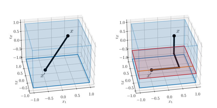
Figure 1: A visual comparison of existing approaches (left), and the proposed approach (right) in $\mathbb{R}^{3}$, with $X=[-1,1]^{3}$, $x^{\prime}=[-0.5\ -0.5\ -0.5]^{T}$, and $x=[0.5\ 0.5\ 0.5]^{T}$. Left: using the straight-line path requires $\mathcal{J}$ to include every possible Jacobian matrix $Df(x)$ for $x\in X$. Right: using the element-wise path requires $\mathcal{M}$ to include every possible mixed Jacobian matrix $M_{x^{\prime}}f(x,s)$ for $x\in X$ and $s\in[0,1]^{3}$ (see Definition 1). For a fixed $s\in[0,1]^{3}$, $M_{x^{\prime}}f(x,s)$ consists of the following three columns: $(M_{x^{\prime}}f(x,s))_{:,1}=(Df(-0.5+s_{1},-0.5,-0.5))_{:,1}$, $(M_{x^{\prime}}f(x,s))_{:,2}=(Df(0.5,-0.5+s_{2},-0.5))_{:,2}$, $(M_{x^{\prime}}f(x,s))_{:,3}=(Df(0.5,0.5,-0.5+s_{3}))_{:,3}$.

In this note, given a particular known trajectory $x^{\prime}$, we build a new linear differential inclusion $\dot{\varepsilon}\in\overline{\operatorname{co}}(\mathcal{M})\varepsilon$, bounding the error dynamics of the system between an arbitrary trajectory $x$ and the fixed trajectory $x^{\prime}$, which we subsequently use to study contraction to $x^{\prime}$. The key novelty of our approach is to consider an element-wise path between $x^{\prime}$ and $x$, rather than the straight line connecting them (see Figure 1), which potentially improves contraction estimates when $x^{\prime}$ is known. The set of matrices $\mathcal{M}$ used to construct this LDI is inspired by existing results in the interval analysis literature. A result similar to Corollary 1 was originally proposed in [15] to find solutions to the system of equations $f(x)=0$ and further used to define the mixed centered inclusion function [16, Section 2.4.4], which improves upon a class of Jacobian-based inclusion functions that over-approximates the range of a function using interval bounds of its Jacobian matrix.

One of the features of contraction theory is its generality in comparing any two trajectories of the system, rather than comparing to a known fixed trajectory. For instance, if $c<0$ in (1) (strongly contracting), it can be shown that every trajectory will converge to an a priori unknown unique equilibrium point [2, Theorem 3.9]. However, in many applications of contraction theory, the trajectory $x^{\prime}$ in (1) is fixed to a known trajectory of the system, motivating the setting of this work. For example, in reachable set computation [17, 18, 19], a single trajectory of the system is simulated and a full reachable tube around this trajectory is computed by expanding or contracting a norm ball using an upper bound of the logarithmic norm. For robustness analysis of implicit neural networks [11, 12], contraction theory adds robustness by analyzing a contraction condition around nominal data samples. Finally, contraction has been used to design feedback controllers for trajectory tracking [9], which fix $x^{\prime}$ to the trajectory to be tracked.

Another feature of contraction theory when $c<0$ is the verification of norm-based Lyapunov functions without explicitly computing the time derivative of $V$ [2, Thm. 3.9]. In particular, a negative uniform bound of the logarithmic norm of the Jacobian provides a sufficient condition verifying that $V(x)=|x-x^{\prime}|$ is a Lyapunov function when $x^{\prime}$ is fixed to an equilibrium of the system. As demonstrated in Corollary 2, the new LDI built in this paper retains this feature: a uniform bound of the logarithmic norm of the matrices in $\mathcal{M}$ provides the same sufficient condition, avoiding the need to explicitly compute and verify the time derivative condition on $V$.

The note is structured as follows. In Section 2, we recall how the usual contraction bound (1) equivalently arises through stability analysis of an LDI encompassing the incremental dynamics of the system. In Section 3, we build a similar LDI using our proposed mixed Jacobian operator in Definition 1, where we traverse an element-wise path resulting in a different set of matrices bounding the output of a function. In Section 4, we apply the LDI to study contraction to an a priori known trajectory $x^{\prime}$, where a uniform bound of the logarithmic norm of our new mixed Jacobian matrix set yields a contraction bound. Finally, in Section 5, we use interval analysis to bound the mixed Jacobian matrix, culminating in an improved algorithm for computing ellipsoidal reachable sets.

2 Preliminaries

2.1 Notation

Let $|\cdot|$ denote a norm on $\mathbb{R}^{n}$. For a matrix $A\in\mathbb{R}^{n\times n}$, let $\|A\|=\sup_{x\in\mathbb{R}^{n}:|x|=1}|Ax|$ denote the induced norm on $\mathbb{R}^{n\times n}$. Let $\mu(A)=\lim_{h\downarrow 0}\frac{\|I+hA\|-1}{h}$ denote the (induced) logarithmic norm, also called the matrix measure. For $x\in\mathbb{R}^{n}$, let $|x|_{1}=\sum_{i=1}^{n}|x_{i}|$ denote the $\ell_{1}$-norm, and $\mu_{1}$ be the induced logarithmic norm. For $x\in\mathbb{R}^{n}$ and positive definite $P\succ 0$, let $|x|_{2,P^{1/2}}=\sqrt{x^{T}Px}$ be the $P$-weighted $\ell_{2}$ norm on $\mathbb{R}^{n}$, $\mu_{2,P^{1/2}}$ be its induced logarithmic norm, and $\mathcal{B}_{r}^{P}(x^{\prime}):=\{x\in\mathbb{R}^{n}:|x-x^{\prime}|_{2,P^{1/2}}\leq r\}$ be the closed ball of radius $r$ about $x^{\prime}\in\mathbb{R}^{n}$. The following linear matrix inequality (LMI) provides a convex characterization of $\mu_{2,P^{1/2}}$,

$$\mu_{2,P^{1/2}}(M)\leq c\iff M^{T}P+PM\preceq 2cP.$$ (2)

Let $\mathbb{IR}$ denote the set of closed intervals of $\mathbb{R}$, of the form $\{a\in\mathbb{R}:\underline{a}\leq a\leq\overline{a},\ \underline{a},\overline{a}\in\mathbb{R}\cup\{\pm\infty\}\}$. An interval matrix $[\mathcal{S}]\in\mathbb{IR}^{m\times n}$ is a matrix of closed intervals in $\mathbb{R}$, i.e., $[\mathcal{S}]_{ij}\in\mathbb{IR}$. $[\mathcal{S}]$ is a subset of $\mathbb{R}^{m\times n}$ in the entrywise sense, so $A\in[\mathcal{S}]$ is $A_{ij}\in[\mathcal{S}]_{ij}$ for every $i=1,\dots,m$ and $j=1,\dots,n$. Given a set $\mathcal{S}\subseteq\mathbb{R}^{m\times n}$, there is a unique smallest interval $[\mathcal{S}]$ containing $\mathcal{S}$, i.e., $\bigcap_{[\mathcal{S}]\in\mathbb{IR}^{m\times n}:\mathcal{S}\subseteq[\mathcal{S}]}[\mathcal{S}]$. This is well defined since the closed intervals on $\mathbb{R}$ are closed to arbitrary intersection, and $[\mathcal{S}]$ is defined entrywise.

For any map $f$ and any subset $X$, let $f(X)=\{f(x):x\in X\}$ denote the set-valued image of $f$ over $X$. Let $\overline{\operatorname{co}}(X)=\operatorname{cl}(\operatorname{co}(X))$ denote the closed convex hull of $X$. Let $D^{+}$ denote the upper Dini derivative, i.e., $D^{+}f(t)=\limsup_{h\downarrow 0}\frac{f(t+h)-f(t)}{h}$ for a continuous map $f:\mathbb{R}\to\mathbb{R}^{n}$. For a differentiable map $f:\mathbb{R}^{n}\to\mathbb{R}^{m}$, let $Df:\mathbb{R}^{n}\to\mathbb{R}^{m\times n}$ denote the Jacobian map, such that $(Df(x))_{ij}=\frac{\partial f_{i}}{\partial x_{j}}(x)$.

We will make use of the following definitions:

• The system $\dot{x}=f(t,x)$ is contracting at rate $c\in\mathbb{R}$ if for any $t_{0}\in\mathbb{R}$, and any two trajectories $t\mapsto x(t)$ and $t\mapsto x^{\prime}(t)$ each defined on $[t_{0},\infty)$, for every $t\geq t_{0}$,

  $$|x(t)-x^{\prime}(t)|\leq e^{c(t-t_{0})}|x(t_{0})-x^{\prime}(t_{0})|.$$

• Given a known trajectory $t\mapsto x^{\prime}(t)$ defined on $[t_{0},\infty)$ for some $t_{0}\in\mathbb{R}$, the system $\dot{x}=f(t,x)$ is contracting to $x^{\prime}$ at rate $c\in\mathbb{R}$ if for any trajectory $t\mapsto x(t)$ defined on $[t_{0},\infty)$, for every $t\geq t_{0}$,

  $$|x(t)-x^{\prime}(t)|\leq e^{c(t-t_{0})}|x(t_{0})-x^{\prime}(t_{0})|,$$

2.2 Stability Analysis of LDIs for Contraction Analysis

In this section, we review approaches for stability analysis of LDIs and their connection to contraction analysis. A linear differential inclusion (LDI) is given by [20, p.52]

$$\dot{x}\in\Omega x,\quad x(t_{0})=x_{0},$$ (3)

where $\Omega\subseteq\mathbb{R}^{n\times n}$ is a set of matrices. Any $t\mapsto x(t)$ satisfying (3) is called a trajectory of the LDI.

Stability of the LDI (3) has been well studied in the context of robustness analysis of (time-varying) linear systems under uncertainties [21, 22]. In these settings, $\Omega$ is generally an a priori known polytope of possible parameters, and the goal is to ensure that every possible choice of $A\in\Omega$ leads to stable system behavior. The following lemma recalls a standard result whereby if the logarithmic norm of every matrix $M\in\Omega$ is uniformly bounded by $c$, then any trajectory $x(t)$ of the LDI (3) is norm bounded by a factor of $e^{ct}$.

Lemma 1.

Consider the LDI $\dot{x}\in\Omega x$ and some norm $|\cdot|$ on $\mathbb{R}^{n}$. If $\mu(M)\leq c$ for all $M\in\Omega$, then

$$|x(t)|\leq e^{ct}|x(t_{0})|,$$

for any trajectory $t\mapsto x(t)$ of the LDI.

Lemma 1 can be viewed as a corollary of Coppel’s inequalities; see, e.g., [23, Theorem 27, p. 34].

Lemma 1 and the linear matrix inequality (2) are the essential ingredients for quadratic stability analysis of LDIs, e.g., in [20, Ch. 4 and 5], where the convex criterion is used as a constraint in a semi-definite program. Next, we recall an inclusion obtained using the mean value theorem and ideas from convex analysis.

Proposition 1 ([20, p.55]).

Let $f:\mathbb{R}^{n}\to\mathbb{R}^{m}$ be differentiable and $X\subseteq\mathbb{R}^{n}$ be convex. If $\mathcal{J}\subseteq\mathbb{R}^{m\times n}$ satisfies

$$Df(X)\subseteq\mathcal{J},$$

then

$$f(x)-f(x^{\prime})\in\overline{\operatorname{co}}(\mathcal{J})(x-x^{\prime})$$ (4)

for every $x,x^{\prime}\in X$.

The proof is in [20, Section 4.3.1, p.55]; we provide it here for comparison with that of Theorem 1 in the next Section.

Proof.

Fix $\ell\in\mathbb{R}^{m}$ and $x,x^{\prime}\in X$. Consider the curve $\gamma:[0,1]\to X$, $\gamma(s)=sx+(1-s)x^{\prime}$. Since $\gamma$ is continuous on $[0,1]$ and differentiable on $(0,1)$, applying the mean value theorem, there exists $s^{\prime}\in(0,1)$ such that

$$\ell^{T}(f(\gamma(1))-f(\gamma(0)))=\ell^{T}Df(\gamma(s^{\prime}))(\gamma(1)-\gamma(0)).$$

Since $\gamma(s)\in X$ by convexity of $X$, $Df(\gamma(s^{\prime}))\in\mathcal{J}$. Thus,

$$\ell^{T}(f(x)-f(x^{\prime}))\leq\sup_{J\in\overline{\operatorname{co}}(\mathcal{J})}\ell^{T}J(x-x^{\prime}),$$

which implies that $f(x)-f(x^{\prime})$ belongs to every halfspace containing $\overline{\operatorname{co}}(\mathcal{J})(x-x^{\prime})$, since $\ell$ was arbitrary. But since $\overline{\operatorname{co}}(\mathcal{J})(x-x^{\prime})$ is closed and convex, it equals the the intersection of these halfspaces, leading to (4). ∎

Lemma 1 and Proposition 1 recover a standard result from infinitesimal contraction theory. Consider the system

$$\dot{x}=f(x),$$

for $x\in\mathbb{R}^{n}$, $f:\mathbb{R}^{n}\to\mathbb{R}^{n}$ continuously differentiable, and let $X\subseteq\mathbb{R}^{n}$ be a convex set. If $Df(X)\subseteq\mathcal{J}$, then Proposition 1 builds the following LDI,

$$\dot{\varepsilon}=f(x)-f(x^{\prime})\in\overline{\operatorname{co}}(\mathcal{J})(x-x^{\prime})=\overline{\operatorname{co}}(\mathcal{J})\varepsilon,$$

for any $x,x^{\prime}\in\mathbb{R}^{n}$, and $\varepsilon=x-x^{\prime}$. Let $\sup_{J\in\mathcal{J}}\mu(J)\leq c$. By convexity of $\mu$, we also have $\sup_{J\in\operatorname{co}(\mathcal{J})}\mu(J)\leq c$, and by continuity of $\mu$ we also have $\sup_{J\in\overline{\operatorname{co}}(\mathcal{J})}\mu(J)\leq c$. Applying Lemma 1, we therefore see that

$$\sup_{x\in X}\mu(Df(x))\leq c\implies|x(t)-x^{\prime}(t)|\leq e^{ct}|x_{0}-x^{\prime}_{0}|,$$

where $t\mapsto x(t)$, $t\mapsto x^{\prime}(t)$ are the trajectories from initial conditions $x_{0},x^{\prime}_{0}$ at time $0$. In other words, a uniform bound $c$ for the logarithmic norm $\mu(Df(x))$ implies that the system $\dot{x}=f(x)$ is contracting at rate $c$. In the contraction literature, this result has been proved in several other ways, including integrating along the line segment $\gamma$ connecting $x^{\prime}$ and $x$ [4, Lemma 1], [1, Lemma 2], verifying a Finsler-Lyapunov condition on the tangent bundle [8, 24], and using weak pairings compatible with the norm [13].

In the next section, we show how the LDI viewpoint allows for a modification when $x^{\prime}$ is fixed to a known trajectory.

3 The Mixed Jacobian Linear Inclusion for Differentiable Mappings

In this section, we build a new linear inclusion that characterizes the behavior of a general differentiable map $f:\mathbb{R}^{n}\to\mathbb{R}^{m}$ when comparing an arbitrary $x\in\mathbb{R}^{n}$ to a fixed $x^{\prime}\in\mathbb{R}^{n}$. As with the linear inclusion from Proposition 1, our inclusion is built using first-derivatives of the function $f$.

3.1 The Mixed Jacobian for the New Linear Inclusion

In order to define the linear inclusion, we first define a new differential operator constructing a matrix with a particular structure in its partial derivative evaluations.

Definition 1 (Mixed Jacobian matrix).

Given $x^{\prime}\in\mathbb{R}^{n}$, define the mixed Jacobian operator $M_{x^{\prime}}$, such that for differentiable $f:\mathbb{R}^{n}\to\mathbb{R}^{m}$, $M_{x^{\prime}}f:\mathbb{R}^{n}\times[0,1]^{n}\to\mathbb{R}^{m\times n}$ where

$$( M_{x^{\prime}}f(x,s))_{ij}$$

$$=\frac{\partial f_{i}}{\partial x_{j}}(x_{1},\dots,x_{j-1},s_{j}x_{j}+(1-s_{j})x^{\prime}_{j},x^{\prime}_{j+1},\dots,x^{\prime}_{n}).$$

The matrix $M_{x^{\prime}}f(x,s)$ is called the mixed Jacobian matrix of $f$ at $(x,s)$, since it mixes the inputs to the Jacobian between the point $x^{\prime}$ and $x$.

In the following Theorem, we present the first contribution of this work: a new linear inclusion bounding the behavior of a differentiable map $f$. As seen in its proof, the set of mixed Jacobian matrices between $x^{\prime}$ and $x$ characterizes the partial derivatives along an elementwise path between them.

Theorem 1.

Let $f:\mathbb{R}^{n}\to\mathbb{R}^{m}$ be differentiable, $X\subseteq\mathbb{R}^{n}$, and consider some fixed $x^{\prime}\in X$. If $\mathcal{M}\subseteq\mathbb{R}^{m\times n}$ satisfies

$$M_{x^{\prime}}f(X,[0,1]^{n})\subseteq\mathcal{M},$$

then

$$f(x)-f(x^{\prime})\in\overline{\operatorname{co}}(\mathcal{M})(x-x^{\prime})$$ (5)

for every $x\in X$.

Proof.

Fix $\ell\in\mathbb{R}^{m}$ and $x\in X$. For each $k=1,\dots,n$, consider the curve $\gamma_{k}:[0,1]\to\mathbb{R}^{n}$,

$$\gamma_{k}(s)=[x_{1}\cdots x_{k-1}\ sx_{k}+(1-s)x^{\prime}_{k}\ x^{\prime}_{k+1}\cdots x^{\prime}_{n}]^{T}.$$

Each curve $\gamma_{k}$ is continuous on $[0,1]$ and differentiable on $(0,1)$, thus using the mean value theorem there exists $s_{k}\in(0,1)$ such that

$$\ell^{T} (f(\gamma_{k}(1))-f(\gamma_{k}(0)))=\ell^{T}(Df(\gamma(s_{k}))(\gamma_{k}(1)-\gamma_{k}(0)))$$

$$=\ell^{T}\sum_{j=1}^{n}\frac{\partial f}{\partial x_{j}}(\gamma_{k}(s_{k}))((\gamma_{k}(1))_{j}-(\gamma_{k}(0))_{j}).$$

Note that $\gamma_{k}(1)=[x_{1}\cdots x_{k}\ x^{\prime}_{k+1}\cdots x^{\prime}_{n}]^{T}=\gamma_{k+1}(0)$ for every $k=1,\dots,n-1$. Thus, summing over $k=1,\dots,n$, the LHS is telescoping. Swapping the order of summation on the RHS, we see that

$$\ell^{T} (f(\gamma_{n}(1))-f(\gamma_{1}(0)))=\ell^{T}(f(x)-f(x^{\prime}))$$

$$=\ell^{T}\sum_{j=1}^{n}\sum_{k=1}^{n}\frac{\partial f}{\partial x_{j}}(\gamma_{k}(s_{k}))((\gamma_{k}(1))_{j}-(\gamma_{k}(0))_{j})$$

$$=\ell^{T}\sum_{j=1}^{n}\frac{\partial f}{\partial x_{j}}(\gamma_{j}(s_{j}))(x_{j}-x^{\prime}_{j}),$$ (6)

where (6) follows since $(\gamma_{k}(1))_{j}-(\gamma_{k}(0))_{j}=x_{j}-x_{j}=0$ if $j\leq k-1$, $(\gamma_{k}(1))_{j}-(\gamma_{k}(0))_{j}=x^{\prime}_{j}-x^{\prime}_{j}=0$ if $j\geq k+1$, and $(\gamma_{k}(1))_{j}-(\gamma_{k}(0))_{j}=x_{j}-x^{\prime}_{j}$ when $j=k$. Finally, since $\gamma_{j}(s_{j})=[x_{1}\cdots x_{j-1}\ s_{j}x_{j}+(1-s_{j})x^{\prime}_{j}\ x^{\prime}_{j+1}\cdots x^{\prime}_{n}]$,

$$\ell^{T}(f(x)-f(x^{\prime})) =\ell^{T}\sum_{j=1}^{n}(M_{x^{\prime}}f(x,s))_{:,j}(x_{j}-x^{\prime}_{j})$$

$$\leq\sup_{M\in\overline{\operatorname{co}}(\mathcal{M})}\ell^{T}M(x-x^{\prime}),$$

since $M_{x^{\prime}}f(x,s)\in\mathcal{M}$. Thus, $f(x)-f(x^{\prime})$ belongs to every halfspace containing $\overline{\operatorname{co}}(\mathcal{M})(x-x^{\prime})$, since $\ell$ was arbitrary. But since $\overline{\operatorname{co}}(\mathcal{M})(x-x^{\prime})$ is closed and convex, it equals the the intersection of these halfspaces, leading to (5). ∎

The key feature of the proof of Theorem 1 is the particular path constructed from $x^{\prime}$ to $x$. Instead of traversing the straight line segment as in Proposition 1, we construct a path which only changes along one coordinate at a time (see Figure 1 for a visualization). Repeated application of the mean value theorem on these $n$ different segments builds the vector $s\in[0,1]^{n}$, characterizing $n$ different points along the elementwise path. The mixed Jacobian matrix $M_{x^{\prime}}f(x,s)$ carries the corresponding Jacobian column at each of these $n$ points.

3.2 Interval Overapproximations of the (Mixed) Jacobian

In either Proposition 1 or Theorem 1, a natural question is how to build a matrix set $\mathcal{J}$ and $\mathcal{M}$ satisfying the stated assumptions. Analytically, it may be possible to write, in closed form, the true image of the Jacobian operator $Df(X)$ or the mixed Jacobian operator $M_{x^{\prime}}(X,[0,1]^{n})$. This approach is used in the next section for Examples 2 and 3.

For automated analysis, a closed form expression for the true images may be difficult to derive. Instead, a more tractable approach may be to construct a set overapproximating the true image. For instance, the approach developed in [25, 26] uses interval analysis [16] to obtain an interval matrix $[\mathcal{J}]$ overapproximating the set $Df(X)$. Interval analysis propagates interval overapproximations through functional building blocks to automatically bound each entry of the Jacobian matrix into their own intervals as $\frac{\partial f_{i}}{\partial x_{j}}(X)\subseteq[\mathcal{J}]_{ij}$. Analogously, one can also use interval analysis to compute an interval matrix $[\mathcal{M}]$ containing the image of the mixed Jacobian operator. The following Corollary shows how to build an interval matrix $[\mathcal{M}]$ containing the mixed Jacobian matrices, which coincides with the mixed Jacobian interval matrix from [15, 16]. Further, the smallest interval matrix $[\mathcal{M}]$ is always smaller than the smallest interval matrix $[\mathcal{J}]$ on an interval initial set.

Corollary 1 (Interval approximations).

Let $f:\mathbb{R}^{n}\to\mathbb{R}^{m}$ be differentiable, $X=X_{1}\times\cdots\times X_{n}\in\mathbb{IR}^{n}$ be an interval, and consider some fixed $x^{\prime}\in X$. The following statements hold:

1. An interval matrix $[\mathcal{J}]$ satisfies $Df(X)\subseteq[\mathcal{J}]$ if for every $i=1,\dots,m$ and $j=1,\dots,n$,

   $$\frac{\partial f_{i}}{\partial x_{j}}(X_{1},\dots,X_{j},X_{j+1},\dots,X_{n})\subseteq[\mathcal{J}]_{ij};$$ (7)

2. An interval matrix $[\mathcal{M}]$ satisfies $M_{x^{\prime}}f(X,[0,1]^{n})\subseteq[\mathcal{M}]$ if for every $i=1,\dots,m$ and $j=1,\dots,n$,

   $$\frac{\partial f_{i}}{\partial x_{j}}(X_{1},\dots,X_{j},x^{\prime}_{j+1},\dots,x^{\prime}_{n})\subseteq[\mathcal{M}]_{ij}.$$ (8)

Moreover, the smallest interval matrices $[\mathcal{J}]$ and $[\mathcal{M}]$ satisfying (7) and (8) respectively also satisfy $[\mathcal{M}]\subseteq[\mathcal{J}]$.

Proof.

The statement (i) is clear, as interval matrix inclusion is elementwise. Regarding statement (ii), since $X$ is an interval, any $x\in X$ and $s\in[0,1]^{n}$ satisfies that $[x_{1}\cdots x_{j-1}\ (1-s_{j})x_{j}+s_{j}x^{\prime}_{j}\ x^{\prime}_{j+1}\cdots x^{\prime}_{n}]^{T}\in X$ for every $j=1,\dots,n$. Thus, $[\mathcal{M}]$ satisfies $M_{x^{\prime}}(X,[0,1]^{n})\subseteq[\mathcal{M}]$. Lastly, $[\mathcal{J}]$ clearly satisfies (8) since $x^{\prime}_{j}\in X_{j}$ for every $j$, so if $[\mathcal{M}]$ is the smallest interval matrix satisfying (8), then $[\mathcal{M}]\subseteq[\mathcal{J}]$. ∎

The key improvement in using the mixed Jacobian operator is shown in (8), where for the $j$-th column, the last $j+1$ through $n$ inputs are fixed to $x^{\prime}_{j+1}$ through $x^{\prime}_{n}$, rather than the entire intervals $X_{j+1}$ through $X_{n}$ as (7). Obtaining interval matrices satisfying (7) or (8) given differentiable $f$ is automatic using interval analysis toolboxes such as immrax [27].

Remark 1 (Connection to interval analysis literature).

Our bound in Theorem 1 is inspired by known results in the interval analysis literature, and Corollary 1 (for interval matrices $[\mathcal{M}]$) is essentially equivalent to the result from [15]. The focus in [15] is in finding solutions to the system of equations $f(x)=0$, rather than analyzing the nonlinear dynamical system $\dot{x}=f(x)$. The interval matrix $[\mathcal{M}]$ has also been used to construct interval inclusion functions in [16] for robustness analysis of the map $f$.

Remark 2 (Interval overapproximations).

More generally, $[\mathcal{M}]\subseteq[\mathcal{J}]$ in Corollary 1 whenever an inclusion monotonic inclusion function [16, Section 2.4] of $\frac{\partial f_{i}}{\partial x_{j}}$ is used to obtain the entrywise bounds from (7) and (8). In particular, most interval methods build such inclusion functions through composition of inclusion monotonic building blocks.

4 Contraction Analysis to Known Trajectories

In this section, we apply the inclusion from Theorem 1 to study contraction of nonlinear systems to known trajectories. Consider the following time-varying nonlinear system

$$\dot{x}=f(t,x)=f_{t}(x),\quad x(t_{0})=x_{0},$$ (9)

where $f:\mathbb{R}\times\mathbb{R}^{n}\to\mathbb{R}^{n}$ is continuous, with continuous partial derivatives with respect to $x$, i.e., $(t,x)\mapsto\frac{\partial f}{\partial x}(t,x)$ is continuous. Let $f_{t}:\mathbb{R}^{n}\to\mathbb{R}^{n}$ denote $x\mapsto f_{t}(x)=f(t,x)$.

4.1 Contraction to a Known Trajectory

Mirroring the analysis from Section 2.2, the following Theorem uses a uniform bound of the logarithmic norm of the mixed Jacobian matrices to construct the usual contraction bound between arbitrary trajectories $x$ and the particular known trajectory $x^{\prime}$ of the system (9).

Theorem 2.

Let $|\cdot|$ be a norm with induced logarithmic norm $\mu$, and let $X\subseteq\mathbb{R}^{n}$ be a set. Consider the dynamical system $\dot{x}=f_{t}(x)$ from (9). Let $t\mapsto x^{\prime}(t)\in X$ be a known trajectory defined on $[t_{0},\infty)$. If for some $c\in\mathbb{R}$,

$$\sup_{t\in[t_{0},\infty),\,x\in X,\,s\in[0,1]^{n}}\mu(M_{x^{\prime}(t)}f_{t}(x,s))\leq c,$$

then the system is contracting to $x^{\prime}$ at rate $c$, i.e., for any trajectory $t\mapsto x(t)\in X$ defined on $[t_{0},\infty)$,

$$|x(t)-x^{\prime}(t)|\leq e^{c(t-t_{0})}|x(t_{0})-x^{\prime}(t_{0})|,$$

for every $t\geq t_{0}$.

Proof.

For every $t\geq t_{0}$, set $\mathcal{M}_{t}:=M_{x^{\prime}(t)}f(X,[0,1]^{n})$. Letting $\varepsilon=x-x^{\prime}$, we observe that

$$\dot{\varepsilon}(t)=\dot{x}(t)-\dot{x}^{\prime}(t)=f_{t}(x(t))-f_{t}(x^{\prime}(t)),$$

for any $t\geq t_{0}$ since $x$ and $x^{\prime}$ are trajectories. Applying Theorem 1 to the map $f_{t}:\mathbb{R}^{n}\to\mathbb{R}^{n}$, since $x(t),x^{\prime}(t)\in X$, for every $t\geq t_{0}$,

$$\dot{\varepsilon}(t)\in\overline{\operatorname{co}}(\mathcal{M}_{t})\varepsilon(t).$$ (10)

Fix $t\geq t_{0}$. Equation (10) implies that for every $\tau\in[t_{0},t]$,

$$\dot{\varepsilon}(\tau)\in\underbrace{\left(\textstyle\bigcup_{\tau^{\prime}\in[t_{0},t]}\overline{\operatorname{co}}(\mathcal{M}_{\tau^{\prime}})\right)}_{=:\mathcal{N}}\varepsilon(\tau).$$

Claim: $\sup_{\overline{M}\in\mathcal{N}}\mu(\overline{M})\leq c$. Indeed, fix $\overline{M}\in\mathcal{N}$; there exists $\tau\in[t_{0},t]$ such that $\overline{M}\in\overline{\operatorname{co}}(\mathcal{M}_{\tau})$. Let $\{M_{j}\}_{j=1}^{\infty}$ be a sequence satisfying $M_{j}\in\operatorname{co}(\mathcal{M}_{\tau})$ and $M_{j}\to\overline{M}$. Since $\mu$ is convex [2, Lemma 2.11], $\mu(M_{j})\leq c$ for every $j$ since $\sup_{M\in\mathcal{M}_{\tau}}\mu(M)\leq c$ by assumption. Since $\mu$ is continuous,

$$\mu(\overline{M})=\lim_{j\to\infty}\mu(M_{j})\leq\sup_{j\geq 1}\mu(M_{j})\leq c.$$

Applying Lemma 1 to the LDI $\dot{\varepsilon}=\mathcal{N}\varepsilon$, we arrive at

$$|\varepsilon(t)|\leq e^{c(t-t_{0})}|\varepsilon(t_{0})|.$$

But $t\geq t_{0}$ was arbitrary, completing the proof. ∎

The next Corollary considers the special case of a time-invariant nonlinear system where $x^{\prime}$ is fixed to an equilibrium.

Corollary 2 (Time-invariant exponential stability).

Consider the time-invariant system $\dot{x}=f(x)$ for continuously differentiable $f:\mathbb{R}^{n}\to\mathbb{R}^{n}$. Let $x^{\prime}\in\mathbb{R}^{n}$ such that $f(x^{\prime})=0$, $X\subseteq\mathbb{R}^{n}$ such that $x^{\prime}\in X$. If there exists a $c<0$ satisfying

$$\sup_{x\in X,s\in[0,1]}\mu(M_{x^{\prime}}f(x,s))\leq c<0,$$

then $x^{\prime}$ is a locally exponentially stable equilibrium point, whose basin of attraction includes any forward invariant subset $\mathcal{S}\subseteq X$ containing $x^{\prime}$, with Lyapunov function $V(x)=|x-x^{\prime}|$ satisfying $D^{+}V(x(t))\leq cV(x(t))$ along every trajectory $x$ starting in $\mathcal{S}$.

Proof.

Let $\mathcal{S}\subseteq X$ be a forward invariant subset containing $x^{\prime}$, and let $x(t)$ be any trajectory with initial condition $x_{0}\in\mathcal{S}$. Since $\mathcal{S}$ is forward invariant, $x(t)\in\mathcal{S}\subseteq X$. Since $f$ is time-invariant, $x^{\prime}(t)=x^{\prime}$ is a trajectory. Theorem 2 immediately implies that $V(x(t))\leq e^{c(t-t_{0})}V(x(t_{0}))$ for every $t\geq t_{0}\geq 0$. Thus, considering $x(t)$ and $x^{\prime}(t)$ as the initial conditions and bounding to $t+h$,

$$D^{+}V(x(t)) =\limsup_{h\downarrow 0}\frac{|x(t+h)-x^{\prime}(t+h)|-|x(t)-x^{\prime}(t)|}{h}$$

$$\leq\limsup_{h\downarrow 0}\frac{e^{ch}|x(t)-x^{\prime}(t)|-|x(t)-x^{\prime}(t)|}{h}$$

$$=c|x(t)-x^{\prime}(t)|=cV(x(t)),$$

completing the proof. ∎

Corollary 2 provides another framing of the contribution of this work: first partial derivatives of the vector field $f$ and tools from contraction analysis verify a norm-based Lyapunov condition for the system without explicitly computing the time derivative of $V$. In Examples 1 and 2, we use the mixed Jacobian formulation to verify a quadratic Lyapunov function for a non-contracting system, without explicitly computing $\dot{V}$.

Remark 3 (Comparison to classical contraction).

Theorem 2 retains many of the key features of classical contraction analysis, such as the forgetting of initial conditions when strongly contracting ($c<0$). The main drawback of our approach is that $x^{\prime}$ needs to be known beforehand—considering the set of all possible linearizations $\mathcal{J}$ guarantees the existence of $x^{\prime}$ without knowing it a priori. When $s=0$, $M_{x^{\prime}}f(x,0)=Df(x^{\prime})$, so the Jacobian at $x^{\prime}$ is included in the set $\mathcal{M}$ in Theorem 2. Fixing $x^{\prime}$ is therefore crucial for any benefit from Theorem 2, since letting $x^{\prime}$ vary arbitrarily in $X$ yields the following containment, $M_{X}(X,[0,1]^{n})\supseteq Df(X)$.

Remark 4 (Permuting state variables and varying bases).

Reordering the state variables will result in different element-wise paths taken from $x$ to $x^{\prime}$, generally yielding different mixed Jacobian matrices and potentially different contraction rate guarantees from Theorem 2. Generally, for any basis of $\mathbb{R}^{n}$, a similar path between $x$ and $x^{\prime}$ is constructed by traversing each basis vector direction individually, which computationally corresponds to the same elementwise path in state transformed coordinates.

4.2 Analytical Examples

In this subsection, we demonstrate the advantage of Theorem 2 with two analytical examples.

Example 1.

Consider the system

$$\dot{x}=f(x)=\begin{bmatrix}f_{1}(x)\\ f_{2}(x)\end{bmatrix}=\begin{bmatrix}-x_{1}-\tan^{-1}(x_{1})x_{2}\\ -x_{2}\end{bmatrix}.$$ (11)

This system has a globally asymptotically stable equilibrium at $x^{\prime}=0$, which we prove using Corollaries 1 and 2 with the condition (2) ($P=I$). First, we have

$$Df(x)=\begin{bmatrix}-1-\frac{x_{2}}{1+x_{1}^{2}}&-\tan^{-1}(x_{1})\\ 0&-1\end{bmatrix}.$$

For any interval $X_{1}\times X_{2}\subseteq\mathbb{R}^{2}$, we have

$$\frac{\partial f_{1}}{\partial x_{1}}(X_{1},0) =-1,$$

$$\frac{\partial f_{1}}{\partial x_{2}}(X_{1},X_{2}) =-\tan^{-1}(X_{1})\subseteq[-\pi/2,\pi/2],$$

and trivially $\frac{\partial f_{2}}{\partial x_{1}}(X_{1},0)=0$ and $\frac{\partial f_{2}}{\partial x_{2}}(X_{1},X_{2})=-1$. Therefore, for all $x$, $f(x)\in[\mathcal{M}]x$ where

$$[\mathcal{M}]=\begin{bmatrix}-1&[-\frac{\pi}{2},\frac{\pi}{2}]\\ 0&-1\end{bmatrix}=\operatorname{co}\{M_{+},M_{-}\},\ M_{\pm}=\begin{bmatrix}-1&\pm\frac{\pi}{2}\\ 0&-1\end{bmatrix}.$$

It is easy to check that $M_{+}+M_{+}^{T}\preceq 2cI$ and $M_{-}+M_{-}^{T}\preceq 2cI$ for $c=\left(\frac{\pi}{4}-1\right)<0$, proving that $V(x)=x^{T}x$ is a Lyapunov function with exponential decay rate $\left(\frac{\pi}{4}-1\right)$ by Corollary 2.

In contrast, since $Df(x)$ is triangular and $\frac{\partial f_{1}}{\partial x_{1}}(x)=-1-\frac{x_{2}}{1+x_{1}^{2}}$ can be positive, the system cannot be contracting with respect to any norm.

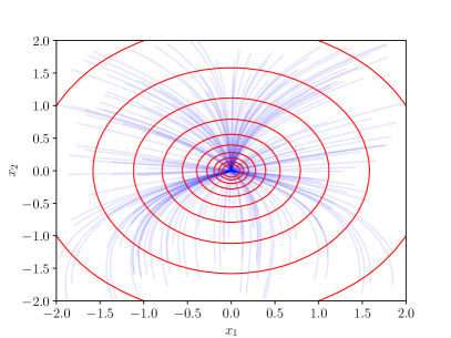
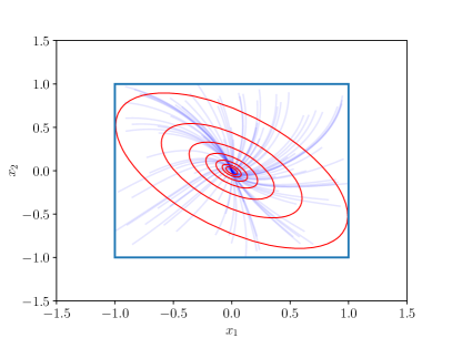
Figure 2: Left (Example 1): Level sets of the Lyapunov function $V(x)=x^{T}x$ from Example 1, verifying global asymptotic stability with exponential decay rate of $c=\frac{\pi}{4}-1$, are shown in red. Sample trajectories are shown in blue. Right (Example 2): Level sets of the local Lyapunov function $V(x)=x^{T}Px$, verifying local asymptotic stability with exponential decay rate of $c=-0.1$, are shown in red. The localizing domain $X=[-1,1]^{2}$ is pictured in light blue, and sample trajectories starting in $X$ are pictured in blue.

Example 2.

Consider the system

$$\dot{x}=f(x)=\begin{bmatrix}f_{1}(x)\\ f_{2}(x)\end{bmatrix}=\begin{bmatrix}-2x_{1}+\frac{1}{2}(x_{1}+x_{2})^{2}\\ -x_{1}+\frac{1}{2}x_{1}^{2}-2x_{2}\end{bmatrix},$$

whose Jacobian matrix is

$$Df(x)=\begin{bmatrix}-2+(x_{1}+x_{2})&1+(x_{1}+x_{2})\\ -1+x_{1}&-2\end{bmatrix}.$$

We verify the exponential stability of $x^{\prime}=0$ and find a region of attraction within the set $X=[-1,1]^{2}$. The mixed Jacobian matrix is

$$M_{x^{\prime}}f(x,s)=\begin{bmatrix}-2+s_{1}x_{1}&1+(x_{1}+s_{2}x_{2})\\ -1+s_{1}x_{1}&-2\end{bmatrix}.$$

First, note that $Df(\begin{bmatrix}1\\ 1\end{bmatrix})=\begin{bmatrix}0&3\\ 0&-2\end{bmatrix}$, so $\mu(Df(\begin{bmatrix}1\\ 1\end{bmatrix}))\geq 0$ for any logarithmic norm $\mu$. Noting that $s_{1}x_{1}\in[-1,1]$ and $(x_{1}+s_{2}x_{2})\in[-2,2]$, $M_{x^{\prime}}f([-1,1]^{2},[0,1]^{2})\subseteq\operatorname{co}\{M_{1},M_{2},M_{3},M_{4}\}$, with

$$M_{1} =\begin{bmatrix}-3&3\\ -2&-2\end{bmatrix},\quad M_{2}=\begin{bmatrix}-3&-1\\ -2&-2\end{bmatrix},$$

$$M_{3} =\begin{bmatrix}-1&3\\ 0&-2\end{bmatrix},\quad M_{4}=\begin{bmatrix}-1&-1\\ 0&-2\end{bmatrix}.$$

Using CVXPY, the following SDP is feasible for $c=-0.1$ and returns $P\approx\begin{bmatrix}1.154&0.747\\ 0.747&1.417\end{bmatrix}$:

$$\min_{P\succeq I}\ \operatorname{trace}(P)\quad\mathrm{s.t.}\quad M_{i}^{T}P+PM_{i}\preceq 2cP\ \forall i\in\{1,2,3,4\}.$$

Thus, $x^{\prime}$ is locally exponentially stable at rate $c=-0.1$, with Lyapunov function $V(x)=|x-x^{\prime}|_{2,P^{1/2}}=x^{T}Px$.

4.3 Contraction to Known Trajectories in the $\ell_{1}$-Norm

When comparing to a fixed trajectory $x^{\prime}$, there are potentially two sources of conservatism when overapproximating the logarithmic norm. When using the full set of possible Jacobian matrices $\mathcal{J}$, no information regarding the comparison point $x^{\prime}$ is used, whereas $\mathcal{M}$ from Theorem 1 uses this information, and in general $Df(x)\notin\mathcal{M}$. However, Theorem 1 requires a mean-value theorem application on $n$ different segments. Each column is built from a Jacobian evaluation at a different location, which means that a matrix $M\in\mathcal{M}$ may not be a Jacobian matrix of the system. To summarize, neither $\mathcal{M}\subseteq\mathcal{J}$ nor $\mathcal{J}\subseteq\mathcal{M}$ are generally true, and as a result, neither will necessarily give better contraction estimates.

In the case of the $\ell_{1}$-norm $|\cdot|_{1}$, however, the column-wise structure allows us to show that using $\mathcal{M}$ from Theorem 2 outperforms the full Jacobian technique that uses $\mathcal{J}$.

Theorem 3.

Let $f:\mathbb{R}^{n}\to\mathbb{R}^{n}$ be differentiable, $X\subseteq\mathbb{R}^{n}$ be an interval, and let $x^{\prime}\in X$. Then

$$\sup_{x\in X,\,s\in[0,1]^{n}}\mu_{1}\left(M_{x^{\prime}}f(x,s)\right)\leq\sup_{x\in X}\mu_{1}\left(Df(x)\right).$$

Proof.

The statement follows by swapping the $\sup$ with the $\max$ from the definition of the $\mu_{1}$ logarithmic norm [2, Table 2.1, p. 27]. Using the shorthand $x_{k:l}=x_{k},\dots,x_{l}$,

$$\sup_{x\in X,\,s\in[0,1]^{n}}\mu_{1}(M_{x^{\prime}}f(x,s))$$

$$=\sup_{x\in X,\,s\in[0,1]^{n}}\max_{j=1,\dots,n}\bigg{\{}M_{x^{\prime}}f(x,s)_{jj}+\sum_{i\neq j}|M_{x^{\prime}}f(x,s)_{ij}|\bigg{\}}$$

$$=\max_{j=1,\dots,n}\sup_{x\in X}\sup_{z_{j}\in\operatorname{co}(x_{j},x^{\prime}_{j})}\bigg{\{}\frac{\partial f_{j}}{\partial x_{j}}(x_{1:j-1},z_{j},x^{\prime}_{j+1:n})$$

$$\quad\quad+\sum_{i\neq j}\left|\frac{\partial f_{i}}{\partial x_{j}}(x_{1:j-1},z_{j},x^{\prime}_{j+1:n})\right|\bigg{\}}$$

$$\leq\max_{j=1,\dots,n}\sup_{x\in X}\bigg{\{}\frac{\partial f_{j}}{\partial x_{j}}(x)+\sum_{i\neq j}\left|\frac{\partial f_{i}}{\partial x_{j}}(x)\right|\bigg{\}}$$

$$=\sup_{x\in X}\max_{j=1,\dots,n}\bigg{\{}\frac{\partial f_{j}}{\partial x_{j}}(x)+\sum_{i\neq j}\left|\frac{\partial f_{i}}{\partial x_{j}}(x)\right|\bigg{\}}=\sup_{x\in X}\mu_{1}(Df(x)),$$

where the inequality holds since $(x_{1:j-1},z_{j},x^{\prime}_{j+1:n})\in X$. ∎

The following example demonstrates Theorem 3.

Example 3.

Consider the system

$$\dot{x}=\begin{bmatrix}f_{1}(x)\\ f_{2}(x)\end{bmatrix}=\begin{bmatrix}-x_{1}\\ -x_{2}-x_{1}x_{2}\end{bmatrix}.$$

We verify the stability of the equilibrium $x^{\prime}=0$ and find a region of attraction. The Jacobian matrix is

$$Df(x)=\begin{bmatrix}-1&0\\ -x_{2}&-1-x_{1}\end{bmatrix},$$

so $\mu_{1}(Df(x))=\max(-1+|x_{2}|,-1-x_{1})$, while $\mu_{1}(M_{x^{\prime}}f(x,s))=\max(-1+|x^{\prime}_{2}|,-1-x_{1})=\max(-1,-1-x_{1})$. On the set $X=\{x\in\mathbb{R}^{2}:x_{1}\geq 0,\ x_{2}\geq 0\}$,

$$\sup_{x\in X}\mu_{1}(Df(x))=+\infty,$$

and in particular, $\mu_{1}(Df(x))<0$ only on the set $\{x\in X:|x_{2}|<1\}$. In contrast, since $x_{1}\geq 0$ on $X$,

$$\sup_{x\in X,s\in[0,1]^{2}} \mu_{1}(M_{x^{\prime}}f(x,s))\leq\max(-1,-1)=-1.$$

$X$ is a forward invariant set by Nagumo’s theorem ($f(x_{1},0)=[-x_{1}\ 0]^{T}$, $f(0,x_{2})=[0\ -x_{2}]^{T}$). Thus, applying Corollary 2, the origin is an exponentially stable equilibrium with region of attraction $X$. In particular, $V(x)=|x|_{1}$ is a Lyapunov function satisfying $D^{+}V(x(t))\leq-V(x(t))$ along any trajectory $t\mapsto x(t)$ with initial condition in $X$. This is also directly verifiable since on the positive quadrant $X$, $V(x)=x_{1}+x_{2}$, so $\dot{V}=-x_{1}-x_{2}-x_{1}x_{2}\leq-(x_{1}+x_{2})=-V$.

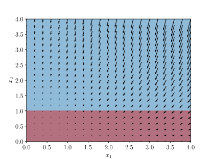
Figure 3: The phase portrait from Example 3 is pictured. The verified region of attraction $X$ is pictured in blue, and the set where $\mu(Df(x))<0$ is pictured in red. While the system is not necessarily infinitesimally $\ell_{1}$-contracting on the blue region $X$, Corollary 2 is able to verify that their $\ell_{1}$-distance to the origin is exponentially decreasing.

5 Application to Ellipsoidal Reachability

An application of contraction analysis is in computing overapproximating reachable sets in nonlinear systems through the following steps: (i) compute a nominal trajectory $x^{\prime}(t)$; (ii) bound the logarithmic norm for some region around $x^{\prime}(t)$; (iii) expand/contract norm balls using this rate [17]. Several variations of this simulation-guided approach have been proposed, but to our knowledge, each of the existing approaches bound the logarithmic norm for the entire Jacobian. One approach uses analytically derived bounds for the logarithmic norm and has been used in the study of switched systems [18] and in component-wise contraction techniques to improve scalability [19]. Another approach automatically computes upper bounds for the logarithmic norm using interval bounds for the Jacobian matrix [25, 26, 28].

From Corollary 1, we recall that the smallest interval matrix $[\mathcal{M}]$ containing $\mathcal{M}$ is a subset of the smallest interval matrix $[\mathcal{J}]$ containing $\mathcal{J}$. Thus, by replacing the interval Jacobian matrix used in [26] with the mixed Jacobian interval matrix from (8), we immediately obtain an improved automated approach to bound the logarithmic norm for reachability analysis. In this section, we provide a basic implementation of the simulation-guided reachability approach, comparing the interval Jacobian to the interval mixed Jacobian.

Algorithm 1 Ellipsoidal $|\cdot|_{2,P^{1/2}}$-norm reachability using mjacM

1:  Input: initial set $\mathcal{B}^{P_{0}}_{1}(x^{\prime}_{0})$, step horizon $\Delta t>0$, number of steps $N\in\mathbb{N}$

2:  $\mathcal{R}\leftarrow\{0\}\times\mathcal{B}^{P_{0}}_{1}(x^{\prime}_{0})$

3:  $x^{\prime}(t)\leftarrow\phi_{t}(x^{\prime}_{0})$ for $t\in[0,N\Delta t]$

4:  for $i=1,\dots,N$ do

5:     $[X_{0}]\leftarrow x^{\prime}(i\Delta t)+[-\sqrt{\operatorname{diag}(P^{-1}_{i-1})},\sqrt{\operatorname{diag}(P^{-1}_{i-1})}]$

6:     Integrate embedding system from $0$ to $\Delta t$, with initial condition $[X_{0}]$, obtaining $\{[X_{t}]\}_{t\in[0,\Delta t]}$

7:     $[\mathcal{M}_{t}]\leftarrow\texttt{mjacM}([X_{t}])$

8:     Obtain $\{M^{j}\}_{j}$ satisfying $\bigcup_{t\in[0,\Delta t]}[\mathcal{M}_{t}]\subseteq\operatorname{co}(\{M^{j}\}_{j})$

9:     $P_{i}\leftarrow\operatorname*{arg\,min}_{P}\log\det(P)$ s.t. $(M^{j})^{T}P+PM^{j}\preceq 2cP$ for all $j$ and $P_{i}\preceq P_{i-1}$, for smallest $c$ (line search)

10:     $\mathcal{R}\leftarrow\mathcal{R}\cup\bigcup_{t\in(0,\Delta t]}\{t+i\Delta t\}\times\mathcal{B}_{e^{ct}}^{P_{i}}(x^{\prime}(t))$

11:     $P_{i}\leftarrow e^{-c\Delta t}P_{i}$

12:  end for

13:  return  Reachable tube $\mathcal{R}$

Suppose an initial set is specified as the ellipsoid $\mathcal{B}_{1}^{P_{0}}(x^{\prime}_{0})$, and let $t\mapsto x^{\prime}(t)$ denote the fixed trajectory from initial condition $x^{\prime}(t_{0})=x^{\prime}_{0}$. The first step of Algorithm 1 is to compute an initial interval over-approximation of the reachable set. In the literature [25], this step has been done using e.g. Lipschitz bounds of the dynamics. Another approach is to use an inclusion function to build an embedding system whose trajectory bounds the behavior of the original system. We use the interval analysis toolbox immrax, which automates the construction of this embedding system, and refer to [27] for a description on how interval analysis constructs these embedding systems for interval reachability.

Since the initial set for Algorithm 1 is an ellipsoid, we overapproximate the ellipsoid with an interval as the initial condition of the embedding system. To do this, we note that

$$\operatornamewithlimits{max}_{x\in\mathbb{R}^{n}:x^{T}Px\leq 1}\ell^{T}x=\sqrt{\ell^{T}P^{-1}\ell},$$

for any $\ell\in\mathbb{R}^{n}$. Thus, taking $\ell\in\{\pm e_{i}\}_{i=1}^{n}$ yields that the smallest interval containing $\mathcal{B}_{1}^{P}(x^{\prime})$ is $[x^{\prime}-\sqrt{\operatorname{diag}(P^{-1})},x^{\prime}+\sqrt{\operatorname{diag}(P^{-1})}]$, where the $\sqrt{\cdot}$ is elementwise.

Given the initial condition $[X_{0}]$, the trajectory of the embedding system obtains an initial coarse interval reachable set $[X_{t}]$, satisfying $x(t)\in[X_{t}]$. The function immrax.mjacM then automatically computes the interval mixed Jacobian matrix $[\mathcal{M}_{t}]$ from Corollary 1 at each time $t$, using automatic differentiation. Once a finite set of corners $\{\mathcal{M}^{j}\}_{j}$ satisfying $\bigcup_{t}[\mathcal{M}_{t}]\subseteq\operatorname{co}(\{\mathcal{M}^{j}\})_{j}$ is chosen, we search for a feasible solution $(c,P)$ satisfying the following constraints,

$$M^{j}P+PM^{j}\preceq 2cP\ \ \forall j, \dagger$$ ()

$$P\preceq P_{0}. \star$$ ()

The condition ($\dagger$ ‣ 5) is the LMI (2) on every corner, implying $\mu_{2,P^{1/2}}(\bigcup_{t}[\mathcal{M}_{t}])\leq c$ by convexity of $\mu$. The condition ($\star$ ‣ 5) ensures the containment of the radius $1$ norm balls as $\mathcal{B}_{1}^{P}(x^{\prime}_{0})\supseteq\mathcal{B}^{P_{0}}_{1}(x^{\prime}_{0})$. Since the constraints are convex only for fixed $c$ or $P$, we settle for a line search over $c$, and a maximization of $\log\det(P)$ to minimize the radius of $\mathcal{B}_{1}^{P}(x^{\prime}_{0})$.

Once a feasible solution $(c,P)$ is found, Theorem 2 ensures that for any trajectory $t\mapsto x(t)$ with initial condition $x(t_{0})\in\mathcal{B}_{1}^{P}(x^{\prime}_{0})$, it follows that $x(t)\in\mathcal{B}^{P}_{e^{c(t-{t_{0}})}}(x^{\prime}(t))$ for every $t\geq t_{0}$. Finally, rescaling back to a radius $1$ ball allows this procedure to iterate to any desired horizon.

Figure 4: The reachable sets from Example 4, comparing $[\mathcal{J}]$ (top) and $[\mathcal{M}]$ (bottom) for varying sizes of initial sets (columns). The ellipsoidal projection onto the $q_{1}$-$q_{2}$ plane is plotted for every $t=0.5k$ (s). The known trajectory $t\mapsto x^{\prime}(t)$ is pictured in black, and several Monte Carlo simulations of the system are pictured in blue. As the initial set increases, overapproximating the logarithmic norm using $[\mathcal{J}]$ yields increasing positive contraction rates, while using $[\mathcal{M}]$ increases the contraction rate but remains negative. $[\mathcal{J}]$ fails for the initial set with radius $r=0.04$.

Example 4 (Robot arm).

We compare to the pure Jacobian-based method from [25], using the $4$-state robot arm model described in [29]

$$\dot{q}_{1} =z_{1},\quad\dot{q}_{2}=z_{2},$$

$$\dot{z}_{1} =\frac{-2mq_{2}z_{1}z_{2}-k_{p_{1}}q_{1}-k_{d_{1}}z_{1}}{mq_{2}^{2}+ML^{2}/3}+\frac{k_{p_{1}}u_{1}}{mq_{2}^{2}+ML^{2}/3},$$

$$\dot{z}_{2} =q_{2}z_{1}^{2}-\frac{k_{p_{2}}q_{2}}{m}-\frac{k_{d_{2}}z_{2}}{m}+\frac{k_{p_{2}}u_{2}}{m},$$

with $u_{1}=k_{p_{1}}$, $u_{2}=k_{p_{2}}$, $M=1$, $L=3$, $k_{p_{1}}=2$, $k_{p_{1}}=1$, $k_{d_{1}}=2$, $k_{d_{2}}=1$.

We run Algorithm 1 with hyperparameters $\Delta t=2$, $N=5$, with varying initial sets $\mathcal{B}_{r}^{P}(x^{\prime}_{0})$ with $P$ and $x^{\prime}_{0}$ from [25], and $r\in\{0.01,0.02,0.04\}$. We order the state variables into the following permutation $[z_{1}\ z_{2}\ q_{1}\ q_{2}]^{T}$ (see Remark 4). For the embedding system integration step at line (6), we use Euler integration with a step size of $h=0.001$. At line (8), we take the interval union of the $\frac{\Delta t}{h}=2000$ interval matrices computed during the integration step, i.e., the smallest interval matrix $[\mathcal{M}]$ containing all $2000$ of these matrices, and sparsely extract the $64$ corners of $[\mathcal{M}]$. There are only $64$ corners since the Jacobian matrix has only $6$ nonconstant elements.

6 Conclusion

In this note, we constructed a new linear differential inclusion bounding the behavior of nonlinear systems by traversing an element-wise path from $x^{\prime}$ to $x$ rather than the traditional straight-line path. When comparing to a known trajectory $x^{\prime}$, this approach provides potential improvement compared to bounding the full Jacobian matrix as in previous approaches. For instance, we demonstrated computational improvement for interval-based algorithms bounding the logarithmic norm for reachability analysis.

References

• [1] Z. Aminzare and E. D. Sontag, “Contraction methods for nonlinear systems: A brief introduction and some open problems,” in 53rd IEEE Conference on Decision and Control, pp. 3835–3847, IEEE, 2014.
• [2] F. Bullo, Contraction Theory for Dynamical Systems. Kindle Direct Publishing, 1.1 ed., 2023.
• [3] A. Davydov and F. Bullo, “Perspectives on contractivity in control, optimization, and learning,” IEEE Control Systems Letters, vol. 8, pp. 2087–2098, 2024.
• [4] E. D. Sontag, “Contractive systems with inputs,” in Perspectives in Mathematical System Theory, Control, and Signal Processing: A Festschrift in Honor of Yutaka Yamamoto on the Occasion of his 60th Birthday, pp. 217–228, Springer, 2010.
• [5] P. DeLellis, M. di Bernardo, and G. Russo, “On quad, lipschitz, and contracting vector fields for consensus and synchronization of networks,” IEEE Transactions on Circuits and Systems I: Regular Papers, vol. 58, no. 3, pp. 576–583, 2010.
• [6] G. Russo, M. Di Bernardo, and E. D. Sontag, “A contraction approach to the hierarchical analysis and design of networked systems,” IEEE Transactions on Automatic Control, vol. 58, no. 5, pp. 1328–1331, 2012.
• [7] W. Lohmiller and J.-J. E. Slotine, “On contraction analysis for non-linear systems,” Automatica, vol. 34, no. 6, pp. 683–696, 1998.
• [8] F. Forni and R. Sepulchre, “A differential lyapunov framework for contraction analysis,” IEEE transactions on automatic control, vol. 59, no. 3, pp. 614–628, 2013.
• [9] I. R. Manchester and J.-J. E. Slotine, “Control contraction metrics: Convex and intrinsic criteria for nonlinear feedback design,” IEEE Transactions on Automatic Control, vol. 62, no. 6, pp. 3046–3053, 2017.
• [10] S. Coogan, “A contractive approach to separable lyapunov functions for monotone systems,” Automatica, vol. 106, pp. 349–357, 2019.
• [11] S. Jafarpour, A. Davydov, A. Proskurnikov, and F. Bullo, “Robust implicit networks via non-euclidean contractions,” in Advances in Neural Information Processing Systems (M. Ranzato, A. Beygelzimer, Y. Dauphin, P. Liang, and J. W. Vaughan, eds.), vol. 34, pp. 9857–9868, Curran Associates, Inc., 2021.
• [12] S. Jafarpour, M. Abate, A. Davydov, F. Bullo, and S. Coogan, “Robustness certificates for implicit neural networks: A mixed monotone contractive approach,” in Proceedings of The 4th Annual Learning for Dynamics and Control Conference, vol. 168 of Proceedings of Machine Learning Research, pp. 917–930, PMLR, 23–24 Jun 2022.
• [13] A. Davydov, S. Jafarpour, and F. Bullo, “Non-euclidean contraction theory for robust nonlinear stability,” IEEE Transactions on Automatic Control, vol. 67, no. 12, pp. 6667–6681, 2022.
• [14] R. G. Sanfelice and L. Praly, “Convergence of nonlinear observers on $\mathbb{R}^{n}$ with a riemannian metric (part i),” IEEE Transactions on Automatic Control, vol. 57, no. 7, pp. 1709–1722, 2012.
• [15] E. Hansen, “On solving systems of equations using interval arithmetic,” Mathematics of Computation, vol. 22, no. 102, pp. 374–384, 1968.
• [16] L. Jaulin, M. Kieffer, O. Didrit, and E. Walter, Applied Interval Analysis. Springer, 1st edition. ed., 2001.
• [17] J. Maidens and M. Arcak, “Reachability analysis of nonlinear systems using matrix measures,” IEEE Transactions on Automatic Control, vol. 60, no. 1, pp. 265–270, 2014.
• [18] J. Maidens and M. Arcak, “Trajectory-based reachability analysis of switched nonlinear systems using matrix measures,” in 53rd IEEE Conference on Decision and Control, pp. 6358–6364, IEEE, 2014.
• [19] M. Arcak and J. Maidens, “Simulation-based reachability analysis for nonlinear systems using componentwise contraction properties,” Principles of Modeling: Essays Dedicated to Edward A. Lee on the Occasion of His 60th Birthday, pp. 61–76, 2018.
• [20] S. Boyd, L. E. Ghaoui, E. Feron, and V. Balakrishnan, Linear Matrix Inequalities in System and Control Theory. SIAM, 1994.
• [21] A. Molchanov and Y. Pyatnitskiy, “Criteria of asymptotic stability of differential and difference inclusions encountered in control theory,” Systems & Control Letters, vol. 13, no. 1, pp. 59–64, 1989.
• [22] T. Hu and F. Blanchini, “Non-conservative matrix inequality conditions for stability/stabilizability of linear differential inclusions,” Automatica, vol. 46, no. 1, pp. 190–196, 2010.
• [23] C. Desoer and M. Vidyasagar, Feedback systems: Input-output properties. Society for Industrial and Applied Mathematics, 1975.
• [24] D. Wu and G.-R. Duan, “Further geometric and lyapunov characterizations of incrementally stable systems on finsler manifolds,” IEEE Transactions on Automatic Control, vol. 67, no. 10, pp. 5614–5621, 2022.
• [25] C. Fan, J. Kapinski, X. Jin, and S. Mitra, “Locally optimal reach set over-approximation for nonlinear systems,” in Proceedings of the 13th International Conference on Embedded Software, pp. 1–10, 2016.
• [26] C. Fan, J. Kapinski, X. Jin, and S. Mitra, “Simulation-driven reachability using matrix measures,” ACM Transactions on Embedded Computing Systems (TECS), vol. 17, no. 1, pp. 1–28, 2017.
• [27] A. Harapanahalli, S. Jafarpour, and S. Coogan, “immrax: A parallelizable and differentiable toolbox for interval analysis and mixed monotone reachability in JAX,” IFAC-PapersOnLine, vol. 58, no. 11, pp. 75–80, 2024. 8th IFAC Conference on Analysis and Design of Hybrid Systems ADHS 2024.
• [28] C. Fan, Automatic simulation-driven reachability using matrix measures. PhD thesis, University of Illinois at Urbana-Champaign, 2016.
• [29] D. Angeli, E. Sontag, and Y. Wang, “A characterization of integral input-to-state stability,” IEEE Transactions on Automatic Control, vol. 45, no. 6, pp. 1082–1097, 2000.