Quantization of Sondheimer oscillations of conductivity in thin cadmium crystals

Abstract

Decades ago, Sondheimer discovered that the electric conductivity of metallic crystals hosting ballistic electrons oscillates with magnetic field. These oscillations, periodic in magnetic field and the period proportional to the sample thickness, have been understood in a semi-classical framework. Here, we present a study of longitudinal and transverse conductivity in cadmium single crystals with thickness varying between 12.6 to 475 $\mu$m. When the magnetic field is sufficiently large or the sample sufficiently thick, the amplitude of oscillation falls off as $B^{-4}$ as previously reported. In contrast, the ten first oscillations follow a $B^{-2.5}e^{-B/B_{0}}$ field dependence and their amplitude is set by the quantum of conductance, the sample thickness, the magnetic length and the Fermi surface geometry. We demonstrate that they are beyond the semi-classical picture, as the exponential prefactor indicates quantum tunneling between distinct quantum states. We draw a picture of these quantum oscillations, in which the linear dispersion of the semi-Dirac band in the cadmium plays a crucial role. The oscillations arise by the intersection between the lowest Landau tube and flat toroids on the Fermi surface induced by confinement. Positive and negative corrections to semi-classical magneto-conductance can occur by alternation between destructive and constructive interference in phase-coherent helical states. The quantum limit of Sondheimer oscillations emerges as another manifestation of Aharanov-Bohm flux quantization.

I Introduction

Confinement of electrons to small spatial dimensions is known to affect electric transport properties [1, 2, 3, 4]. One size effect observed when the thickness of the sample becomes shorter than the bulk mean free path was discovered by Sondheimer [5]. These are oscillations of conductivity, periodic in magnetic field, sometimes dubbed magneto-morphic. Common explanations of Sondheimer oscillations (SO) do not invoke Landau quantification. In contrast, Shubnikov-de Haas oscillations, which are periodic in the inverse of the magnetic field [6], are known to arise because of commensurability in momentum space between the Landau tubes and the extremal areas of the Fermi surface. Sondheimer oscillations are understood to arise due to commensurability between the orbit of the charged carriers in real space and sample thickness. They are thus classified as a semi-classical phenomenon [7].

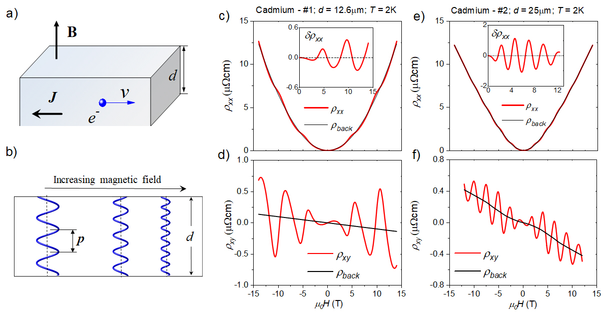
Figure 1: Sondheimer oscillations and their extraction in two thin cadmium crystals. (a) The set-up. Electrons in a metallic solid carry a current in presence of a magnetic field perpendicular to the current. (b) Front view of the electron movement. (c) The field dependence of longitudinal resistivity, $\rho_{xx}$, in 12.6$\mu m$ sample. The red curve is the experimental data and the black line is the oscillatory background. The insert shows the oscillating part after subtracting the background. (d) The Hall resistivity of 12.6$\mu$m sample. (e) The field dependence of longitudinal resistivity, $\rho_{xx}$, in 25$\mu$m sample. The red curve is the experimental data and the black line is the oscillatory background. The insert shows the oscillating part after subtracting the background. (f) The Hall resistivity of 25$\mu$m sample.

Consider a magnetic field perpendicular to an electric current, generating an electric field (Fig. 1a). Because of the Fermi velocity of mobile electrons, there is a Lorentz force on each electron, giving rise to a helical trajectory (Fig. 1b) whose axis is along the magnetic field. With increasing magnetic field, the radius of each turn of the helix decreases. Concomitantly, the distance between these turns (i.e. the size of the helix pitch, $p$) is reduced. At particular values of magnetic field, separated by a fixed period, the thickness ($d$) of the sample becomes an integer number of helix pitches. In ballistic samples, where the mean-free-path limited by disorder is significantly longer than $d$, this leads to oscillations in conductivity, detected by numerous experiments in the second half of the last century [8, 9, 10, 11, 12, 13, 14, 15, 16]. More recently, two studies have been devoted to Sondheimer oscillations in the Weyl semi-metal WP₂ [17] and in graphite [18].

The periodicity of the oscillations can be quantified thanks to a simple expression put forward by Harrison [19] for velocity:

$$v_{z}=\frac{\hbar}{2\pi m^{*}}\frac{\partial A}{\partial k_{z}}$$ (1)

Here, $v_{z}$ and $k_{z}$ represent the Fermi velocity and the wavevector along the magnetic field. $A$ is the cross-section of the Fermi surface in the momentum space perpendicular to the magnetic field. The time for an electron to travel across the thickness is $\tau_{1}=d/v_{z}$. One revolution of the helix takes a time equal to $\tau_{2}=\frac{2\pi m^{\star}}{eB}$. The $\tau_{1}/\tau_{2}$ ratio increases linearly with magnetic field and periodically becomes an integer. At these specific fields, the thickness is an integer number of helical revolutions. The period, $\Delta B$, is therefore given by [3, 8, 20, 7, 17]:

$$\Delta Bd=\frac{\hbar}{e}\frac{\partial A}{\partial k_{z}}.$$ (2)

Sample	$d\times w\times l$ ($\mu$m3)	$\Delta B_{MR}$ (T)	$\Delta B_{Hall}$ (T)	$\rho_{0}$ (n$\Omega$cm)	$\overline{s}=\sqrt{w\times d}$ ($\mu$m )	$\ell_{0}$ ($\mu$m)	$\mu$ (m2/Vs)
$\#$1	12.6 $\times$ 24 $\times$ 70	4.66	4.66	7.37	19.7	29	3.2
$\#$2	25 $\times$ 23 $\times$ 49	2.33	2.4	6.23	23.9	34	5
$\#$3	97.5 $\times$ 160 $\times$ 298	0.58	0.58	2.9	124	80	15
$\#$4	200 $\times$ 170 $\times$ 410	0.27	0.28	1.42	180	160	25
$\#$5	475 $\times$ 362 $\times$ 420	0.12	0.12	1.45	414	155	28

Table 1: Samples used in this study. In all crystals used in this study, the field was oriented along the [0001] axis. $\Delta B_{MR}$ $\Delta B_{Hall}$ represent the oscillation period in the magnetoresistance and the Hall resistivity. $\rho_{0}$ is zero-field resistivity at 2 K. The carrier mean free path $\ell_{0}$ was calculated using $\rho_{0}=\frac{3\pi}{2}\frac{h}{e^{2}}(\left\langle k_{F}\right\rangle^{2}l_{0})^{-1}$, where $\left\langle k_{F}\right\rangle=\frac{n}{3\pi^{2}}$ is the average Fermi wave vector extracted from the carrier density, $n$. In the thickest samples, $\ell_{0}$ is limited by defect scattering and is about 150 $\mu$m. In thinner samples, where $\overline{s}$ is shorter than this, one finds $\ell_{0}\simeq\overline{s}$ and boundary scattering limits the zero-field mean-free-path.

In general, $\partial A/\partial k_{z}$ is not constant as a function of $k_{z}$. Therefore, the existence of a specific periodicity implies a singular value prevailing over the others. An extremum occurs when $\partial^{2}A/\partial k_{z}^{2}\sim 0$ [17, 7]. Semi-classic theory has linked the field dependence of oscillations to the curvature of the Fermi surface [3]. Hurd [7] enumerated four different types. A first type, expected in a spherical or an ellipsoidal Fermi surface, has an amplitude falling off as $B^{-4}$. This is the behavior reported in cadmium and zinc single crystal [8, 11, 12, 13, 21, 22, 23, 24, 25, 26]. A second type, associated with an inflection point, is expected to fall off as $B^{-2.5}$ [27, 7] and has been reported in aluminum single crystals [9, 10]. A third type, expected in a discontinuous or truncated Fermi surface, gives a $B^{-3}$ field dependence. The last type of oscillation associated with a ‘monochromatic’ Fermi surface is expected to fall off as $B^{-2}$ [28, 3, 7].

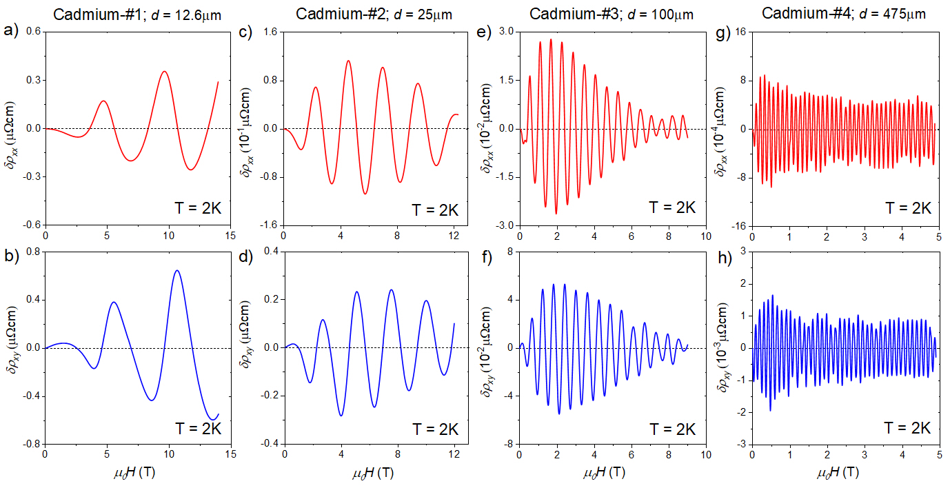
Figure 2: The evolution of Sondheimer oscillations with thickness. (a),(b) The amplitude of SO for longitudinal and transverse resistivity in 12.6 $\mu$m sample, respectively. As the field increasing, the amplitude of oscillation increases. (c),(d) The amplitude of SO for longitudinal and transverse resistivity in 25 $\mu$m sample, respectively. (e),(f) The amplitude of SO for longitudinal and transverse conductivity in 100 $\mu$m sample, respectively. (g),(f) The amplitude of SO for longitudinal and transverse conductivity in 475 $\mu$m sample, respectively.

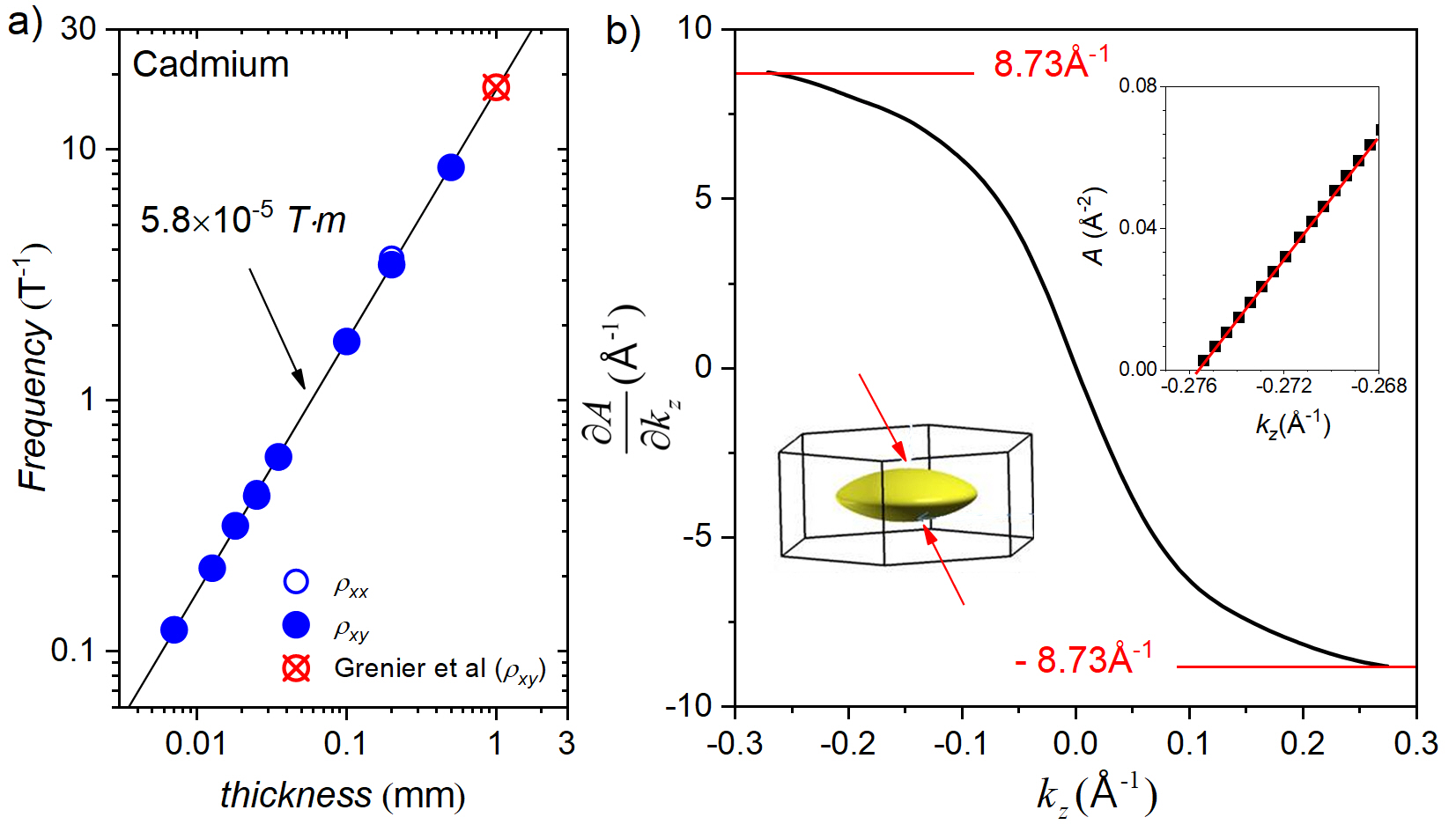
Figure 3: Thickness dependence of oscillation frequency and the Fermi surface topology. (a) Oscillation frequency as a function of thickness. The solid line represents a linear variation with a slope corresponding to: $\Delta B\cdot d=0.058$ T$\cdot$mm, where $\Delta B$ is the period (the inverse of frequency) and $d$ is thickness. We have also included the data point reported by Grenier et al.[8] on a 1.02 mm thick sample. Inserting this $\Delta Bd$ in Equation 2 yields $\frac{\partial A}{\partial k_{z}}=8.76$ Å^-1. (b) The computed $\frac{\partial A}{\partial k_{z}}$ for the non-elliptical electron-like pocket of the Fermi surface of cadmium is shown in the inset. $\frac{\partial A}{\partial k_{z}}=0$ at the equator (where $k_{z}=0$ and $k_{r}=0.742~{}$Å^-1). At the two poles (where $k_{r}=0$ and $k_{z}=\pm 0.275~{}$Å^-1), $\frac{\partial A}{\partial k_{z}}=\pm 8.73$ Å^-1. The disagreement between the experimentally measured and the computed $\frac{\hbar}{e}\times\frac{\partial A}{\partial k_{z}}$ is less than a percent. The lower inset shows the Fermi surface pocket. The upper inset is a plot of $A$ vs. $k_{z}$ near a pole. It is perfectly linear over at least 0.012 Å^-1.

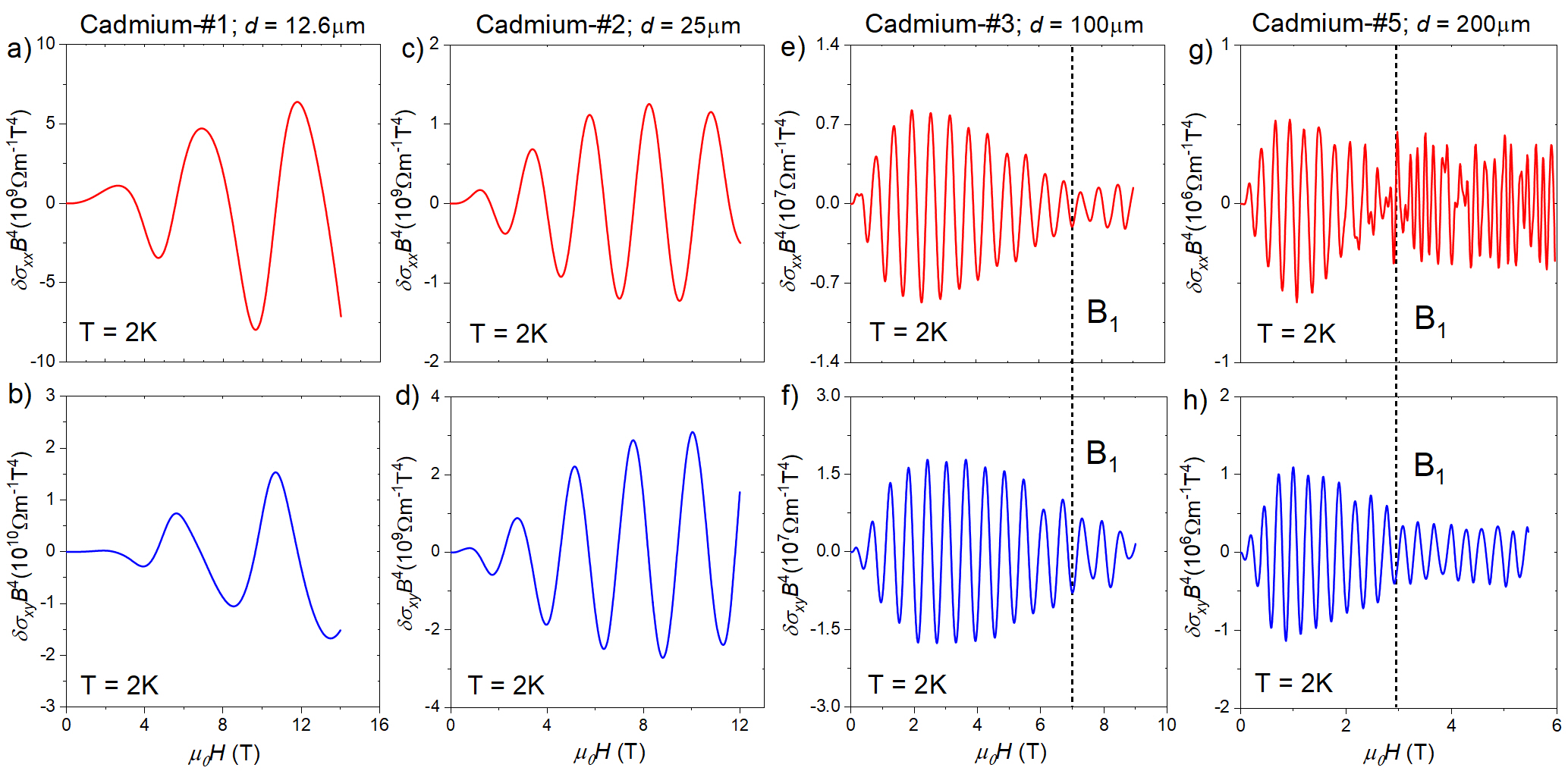
Figure 4: Failure of $B^{-4}$ field dependence. (a),(b) Multiplying longitudinal and transverse conductivity of 12.6 $\mu$m sample by $B^{4}$ does not generate oscillations with constant amplitude. (c),(d) Same observation for the 25 $\mu$m sample. (e),(f) Same for 100 $\mu$m sample, respectively. Note, however, the regime change above 7.1 T. (g),(h) In the 200 $\mu$m sample, when the field exceeds 2.9 T, the amplitude of $\delta\sigma_{xx}B^{4}$ oscillations becomes constant.

Here, we study longitudinal and Hall resistivity of cadmium single crystals with varying thicknesses ($d$), ranging from 12.6 to 475 $\mu$m. Employing focused ion beam (FIB) technology [29] to etch the samples, we have ensured plane and parallel surfaces. Our extensive study on five different samples with a forty-fold variation of thickness leads to solid conclusions regarding the period, the amplitude and the field dependence of oscillations.

The period of oscillations, $\Delta B$, agrees with what was reported by Grenier et al. [8] for a thicker sample. On the other hand, the amplitude of oscillations in thin samples, follows $\delta\sigma\propto B^{-2.5}e^{-B/3\Delta B}$. This is a field dependence, which has never been proposed or observed before. Only when the samples become sufficiently thick, the field dependence becomes $\sigma\propto B^{-4}$ as previously reported. The crossover between the two regimes of field dependence occurs at $\sim 10$ oscillations.

In section II, we present our extensive data and show in detail what leads to the empirical expression of $B^{-2.5}e^{-B/B_{0}}$ as the best fit to the amplitude of oscillations as a function of magnetic field. Then, we show that, normalized by the square of the inverse of the thickness, all curves of conductivity oscillations collapse on top of each other, a forty-fold variation in thickness not withstanding. The result constitutes a rare case of conductivity quantization in three dimensions.

In section III, we contrast our experimental observation of this distinct type of conductivity oscillations with the semi-classical picture and demonstrate that a quantum mechanical treatment is necessary. Recalling that the Larmor radius of semi-classical orbits can never fall below the magnetic length, we argue that a classical-quantum crossover in unavoidable for thin samples at low magnetic field. In absence of a quantum theory, we sketch a rudimentary picture, in which confinement sculpts steps and flat toroids on the Fermi surface. Oscillations arise by successive intersections between the lowest Landau tube and the flat toroids. This picture, drawn in reciprocal space, leads to an expression for the period of oscillations identical to the semi-classical one. In contrast to the latter, however, it allows for constructive and destructive interferences between phase coherent helical states and therefore positive and negative corrections to semiclassical magnetoconductivity. We propose that the exponential prefactor is caused by quantum tunneling between the Fermi Sea and the helical states and identify a promising candidate as the relevant tunneling action. Our picture confirms Chambers’ conjecture [3] regarding a role played by the phase of the electronic wave-function. Most probably, this role is crucial in the quantum regime. A rigorous theoretical account of our results remains a challenge to theory.

II Results

II.1 Samples

The crystal growth and the fabrication of the samples with FIB are discussed in detail in the supplement (Note 1) [30]. Table 1 lists the samples used in this study. Their thickness was varied by a factor of 40. In the thickest samples, the zero-field resistivity at 2 K, was found to be as low as $\sim 1.5$ n$\Omega$cm, implying a mean free path as long as $\sim$150 $\mu$m. This corresponds to the mean free path set by the distance between defects. In samples thinner than 150 $\mu$m, the residual resistivity increases because of the ballistic limit on the mean-free-path. In this regime, the mean-free-path extracted from the zero-field conductivity is comparable to the geometric average of thickness and width of the sample.

II.2 Extracting the oscillating component of the conductivity

Fig.1c and 1d show the data for our thinnest samples, with a thickness of $12.6~{}\mu$m. As seen in Fig.1c, longitudinal resistivity is dominated by a large background. Cadmium is a compensated metal, with a finite overlap between the conduction and the valence bands and an equal density of holes and electrons. Like other elemental semi-metals, such as bismuth [31] and antimony [32], it hosts a large orbital magnetoresistance, which, thanks to perfect compensation, does not saturate even in the high field limit ($\mu B\gg 1$) [33]. On top of this background, one can detect oscillations. The inset shows the oscillating signal extracted by using a quadratic fit to the monotonic background. Two oscillations and the beginning of the third one are clearly visible.

Fig.1d shows the Hall resistivity of the same sample. Here, one can see that field-periodic oscillations dominate the response, which is not surprising given the almost perfect compensation between the density of electrons and holes. The slope of the red solid line implies a finite non-oscillating Hall resistivity. This small residual Hall resistivity indicates a slightly larger mobility for electrons compared to holes.

Fig.1e and Fig.1f show similar data for a twice thicker ($d=25~{}\mu$m) sample. There are twice more oscillations in the same field window and the frequency of oscillations become twice faster. The amplitude of oscillations is also reduced. The shape of oscillations is close to sinusoidal, but the evolution of the amplitude with magnetic field is complex.

Raw data for two thicker samples are shown in the supplement (supplementary notes 2) [30]. They confirm features seen in the thinnest samples.

II.3 Period of oscillations

Fig.2 displays the evolution of the signal in four Cd single crystals with $d$ ranging from 12.5 to 475 $\mu$m. Note the change in the units of vertical and horizontal axes. The absolute amplitude of oscillations and their period both enhance with thinning. Since oscillations are squeezed in thicker samples, the field axis is limited to a lower bound to make them visible. More than one frequency may be present in the thickest ($d=475~{}\mu$m) sample. Here, we will focus on the main one.

The evolution of the main frequency as a function of the thickness is shown in Figure 3a. One can see that our data for $10~{}\mu$m $<d<500~{}\mu$m is in excellent agreement with what was found by Grenier et al. [8] on a sample with $d=1020~{}\mu$m. The red solid line represents a linear relation between thickness and frequency. The product of period and thickness is constant ($\Delta B\cdot d=$ 0.058 T$\cdot$mm) even when $d$ varies by two orders of magnitude. Inserting this in Equation 2 leads to $\frac{\partial A}{\partial k_{z}}$ = 8.76 Å^-1. This is to be compared with what is calculated by ab initio theory $\frac{\partial A}{\partial k_{z}}$=8.73 Å^-1 [34] (See Fig. 3b). The agreement is remarkable. It is noteworthy that the semi-Dirac nature of the band giving rise to the electron-like pocket renders $\frac{\partial A}{\partial k_{z}}$ constant over a significant portion of the Fermi surface near the poles (See the inset of Fig.3b). This will play a crucial role in our analysis.

II.4 Amplitude of oscillations

To compare the amplitude of oscillations with theoretical expectations, we inverted the measured resistivity tensor and quantified the conductivity tensor. Fig.4 displays $\delta\sigma_{xx}B^{4}$ and $\delta\sigma_{xy}B^{4}$ as a function of magnetic field in four samples. By plotting the data in this way one can see that the postulated $\propto B^{-4}$ field dependence does not hold and $\sigma_{ij}B^{4}$ oscillation peaks do not keep a fixed amplitude.

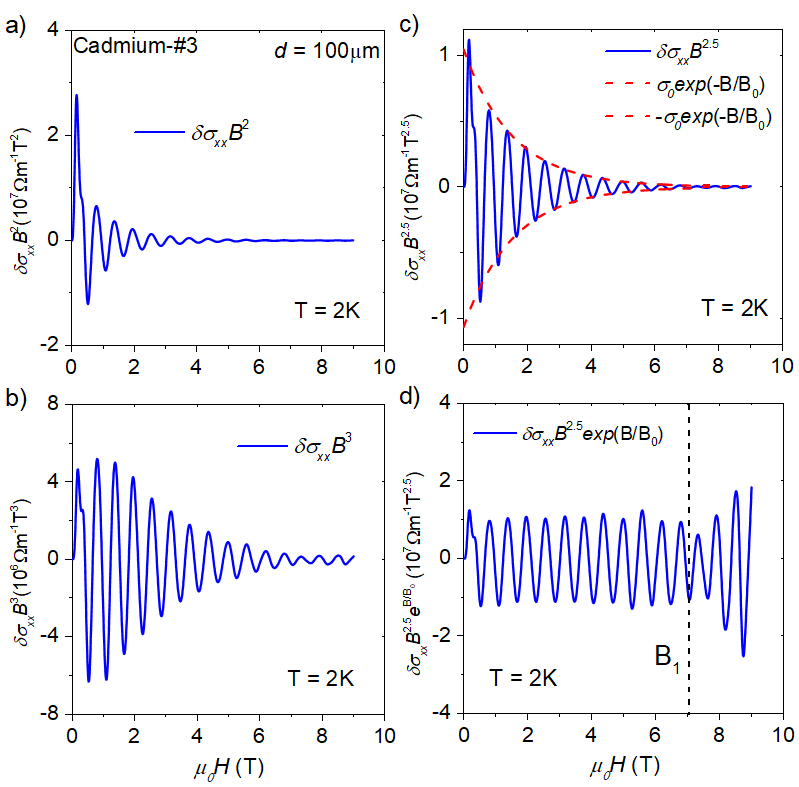
Figure 5: Oscillation falls off as $B^{-2.5}$$e^{B/B_{0}}$. (a) Longitudinal conductivity multiples the $B^{2}$ without an equal amplitude oscillations occurred. (b) Longitudinal conductivity multiples the $B^{3}$ without an equal amplitude oscillations occurred. (c) When conductivity is multiplied by $B^{2.5}$, the result decays exponentially (indicated by the red line). Additionally, an exponential term in the result from the $B^{2.5}$ case produces sinusoidal oscillations (d).

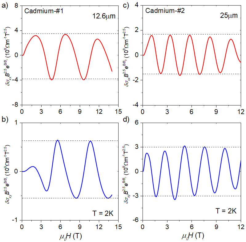
Figure 6: $B^{-2.5}$$e^{-B/B_{0}}$ dependence of the amplitude in thinner samples. (a) The longitudinal conductivity of the 12.6 $\mu$m sample multiplied by $B^{2.5}e^{B/B_{0}}$. Sinusoidal oscillations are observed with a period of 5.14 T. Here, the $B_{0}$ equals 15.2 T. (b) The same result is obtained for Hall conductivity. $B_{0}$ is approximately 16.3 T. (c), (d) Using the same method for 25 $\mu$m sample, sinusoidal oscillations are observed with a period of approximately 2.42 T. $B_{0}$ is 6.8 T and 7.2 T for longitudinal and transverse conductivity.

To empirically explore possible fits to the field dependence of the amplitude of conductivity oscillations, we multiplied the longitudinal conductivity by various powers of the magnetic field. Fig.5 shows the data for the 100 $\mu$m sample. Plots of $\delta\sigma_{xx}B^{\alpha}$ (with $\alpha$ = 2, 2.5 and 3) are shown. None of them are satisfactory. Upon closer examination, we found that $\delta\sigma_{xx}B^{\alpha}$ becomes non-monotonic when $\alpha>2.5$, but is monotonic when $\alpha<2.5$. Moreover, when $\alpha=2.5$, $\delta\sigma_{xx}B^{2.5}$ displays an exponential decay (see Fig.5c, indicated by the red line). This led us to try $\propto B^{-2.5}e^{-B/B_{0}}$ (see Fig.5d) with $B_{0}=1.8$ T. Required for dimensional reasons, $B_{0}$ is a parameter indispensable for ensuring an almost perfect sinusoidal behavior. The deviation from this behavior seen at high fields (Fig.5d) is also meaningful.

We tried this $\propto B^{-2.5}e^{-B/B_{0}}$ fit on data obtained for other samples ($d<100~{}\mu$m). As illustrated in Fig.6, in samples with a thickness of 12.6 and 25 $\mu$m, oscillations of conductivity (both longitudinal and transverse) are $\propto B^{-2.5}e^{-B/B_{0}}$ up to the highest magnetic field (B $<$ 14 T). The few oscillations are almost perfectly sinusoidal with no deviation occurring at high magnetic field. In the 200 and 475 $\mu$m samples, conductivities follow $\propto B^{-2.5}e^{-B/B_{0}}$ below a threshold field, which we call $B_{1}$. Above $B_{1}$, both conductivities follow $\propto B^{-4}$ (See the supplementary note 3 [30]).

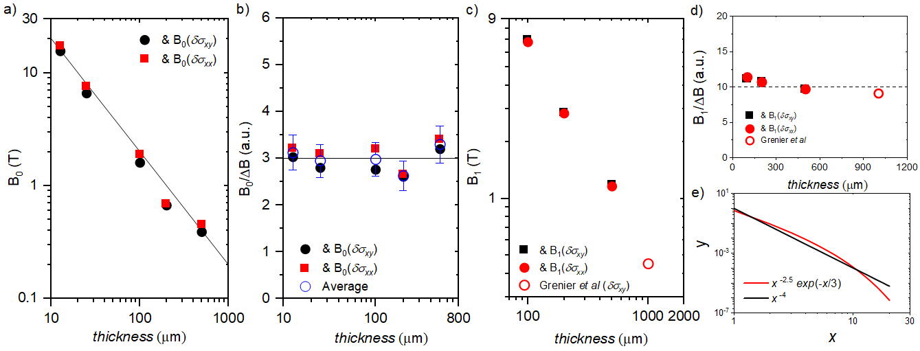
Figure 7: Thickness dependence of $B_{0}$ and $B_{1}$. (a) $B_{0}$ is proportional to the inverse of the thickness. (b) In all samples, $B_{0}$ is about 3 times $\Delta B$. (c) $B_{1}$ is in different samples. It decreases with increasing $t$ increases. The data for $d$ = 1.02 mm is taken from Ref. [8]. (d) The ratio of $B_{1}/\Delta B$ is close to 10 in all samples. (e) A comparison of $g(x)=x^{-4}$ and $f(x)=$exp$(-x/3)x^{-2.5}$. The two functions cross each other at $x^{\star}\simeq 10.5$.

The thickness dependence of $B_{0}$ is shown in Fig.7a. We found that $B_{0}\propto d^{-1}$. As mentioned above, the period of oscillations is also proportional to the inverse of the thickness. As a result, and as can be seen in Fig.7b, the ratio of $B_{0}$ to $\Delta B$ is constant. Even more striking is the fact that in five samples studied, the ratio is close to three: $\frac{B_{0}}{\Delta B}\sim 3$. Thus, $B_{0}$ is not an additional parameter, but is simply three times $\Delta B$. To summarize our results, the field dependence of the amplitude of oscillations has two regimes:

$$\delta\sigma\propto\left\{\begin{array}[]{lr}B^{-2.5}e^{-B/3\Delta B},&B<B_{1}.\\ B^{-4},&B>B_{1}.\end{array}\right.$$ (3)

Let us now turn our attention to the significance of $B_{1}$.

II.5 Boundary between the two regimes

As the sample becomes thicker, the $B_{1}$ threshold field increases. This ensures consistency between our data and what was reported in the previous study of Sondheimer oscillations in cadmium, which was performed on a 1 mm thick sample [8] and concluded that the amplitude of oscillations follows $B^{-4}$. Interestingly, the authors found a deviation from this behavior in their data below $\sim 0.3$ T (See Fig.13 in ref. [8]), in agreement with what is found here.

As seen in Fig. 7c, which shows the thickness dependence of $B_{1}$, the latter is proportional to the inverse of the thickness. The plot includes a data point for $d=1.02$ mm [8] with $B_{1}$ = 0.3 T. Fig. 7d shows that for all samples, $\frac{B_{1}}{\Delta B}\simeq 10$. For more details on the boundary between the two regimes, see the supplementary note 3 [30].

Insight to this is offered by considering the two functions, $g$ and $f$ of $x=B/\Delta B$. With $g(x)=x^{-4}$ and $f(x)=$exp$(-x/3)x^{-2.5}$, one can see that they cross each other at $x^{\star}\simeq 10.5$. In other words, $f>g$ when $x<x^{\star}$ and $f<g$ when $x>x^{\star}$. This means that the $B_{1}=10\Delta B$ is not an independent parameter, but a maker of domination between two competing field dependencies. $\Delta B$ is the unique field scale.

Thus, $\sigma_{ij}\propto B^{-2.5}e^{-B/3\Delta B}\cos(B/\Delta B)$ field dependence, which holds in thinner samples, coexists with the $\sigma_{ij}\propto B^{-4}\cos(B/\Delta B)$ field dependence. The latter dominates in thicker samples and large magnetic field, just because it decays slower at larger fields.

Let us now turn our attention to the thickness dependence.

II.6 Thickness dependence and the quantization of the amplitude

Fig.8 demonstrates that there is a straightforward thickness dependence in the case of the new oscillations observed here. Their amplitude in all cadmium samples studied here can be scaled to collapse on top of each other.

The dimensionless horizontal axis in Fig.8 is the magnetic field multiplied by $\frac{ed}{\hbar}\frac{\partial A}{\partial k_{z}}$. The fact that all curves share the same periodicity implies that the period is described by Equation 2. The vertical axis is the oscillating conductivity divided by the quantum electric conductance $G_{0}=\frac{2e^{2}}{h}$, by exp$(-\frac{B}{3\Delta B})\ell_{B}^{5}$ and then by $d^{-2}$. The curves, expressed in units of Å^-4, superpose. This implies that oscillations are proportional to the inverse of the square of the thickness (See the supplementary note 3 [30] for more plots and details).

Thus, not only the period of the oscillations, but also the amplitude of the first ten oscillations is set by the thickness and the Fermi surface geometry. This scaling implies that the amplitude can be written as:

$$\sigma_{osc}=G_{0}d^{-2}e^{-B/B_{0}}\ell_{B}^{5}k_{s}^{4}$$ (4)

Here, $\ell_{B}=\sqrt{\frac{\hbar}{eB}}$ is the magnetic length. The parameter $k_{s}$ is a length scale in the momentum space. It is set by the Fermi surface geometry. It depends neither on the thickness, nor on the magnetic length. A quantitative account of our result would explain the experimentally observed $k_{s}^{4}\simeq 10$Å^-4.

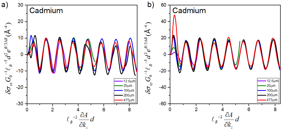
Figure 8: Quantized amplitude of the oscillations (a) Oscillations of normalized conductivity as a function of normalized field. Curves for all samples fall on top of each other. The vertical axis in conductivity divided by the quantum of conductance ($G_{0}=\frac{2e^{2}}{h}$) and multiplied by $\ell_{B}^{-5}d^{2}e^{B/3\Delta B}$. This normalized quantity has the inverse of the length to the power of 4 as its dimension. The horizontal axis is linear in magnetic field. It represents $\ell_{B}^{-2}\times\frac{\partial A}{\partial k_{z}}\times d$. (b) Same for the Hall conductivity data. All curves fall on top of each other and the normalized amplitude is twice larger.

III Discussion

In the previous section, we presented an extensive analysis of our data, which led us to the empirical expression given by Eq. 4. In this section, we will show that this result requires a treatment beyond the semiclassical picture.

III.1 Comparison with semi-classical expectation

It is instructive to compare this expression with what was obtained by Chambers in his semi-classical treatment [3]. Equation 4.41 in ref. [3] can be rewritten as :

$$\sigma_{osc}^{C}=\frac{1}{4}G_{0}k_{F}^{4}\ell_{B}^{8}d^{-3}\beta^{-2}e^{-d/\ell}$$ (5)

Here, $\ell$ is the mean free path and $\beta$ is a length scale in Å, which quantifies the variation of the phase near the extremal point. $k_{F}$ is the relevant radius of the Fermi surface.

Comparing the experimental Eq. 4 with Eq. 5 is instructive. The first striking feature is the two very different exponential functions. The presence of $e^{-d/\ell}$ in Eq. 5 implies a dependence on the thickness and mean free path which does not match what is found by experiment. Note, however, that if one assumes that in ballistic regime $\ell$ is equal to $d$, this exponential becomes a mere numerical prefactor. A more important difference is the presence of $e^{-B/B_{0}}$ in Eq. 4 and its absence in Eq. 5. The presence of this term is a strong signature of a purely quantum origin. Indeed, it is reminiscent of the canonical expression for tunneling between distinct quantum states, which has the form of $e^{-s/\hbar}$ where $s$ is the tunneling action [35]. In the next section, we will come back to this term.

The other differences are less drastic. The two equations become similar if $\beta^{2}\propto\ell_{B}^{3}d$. The presence of $\beta$ in equation 5 suggests that in any scenario for these oscillations, the phase and its variation in reciprocal space play a role.

Let us try an attempt in drawing a quantum picture.

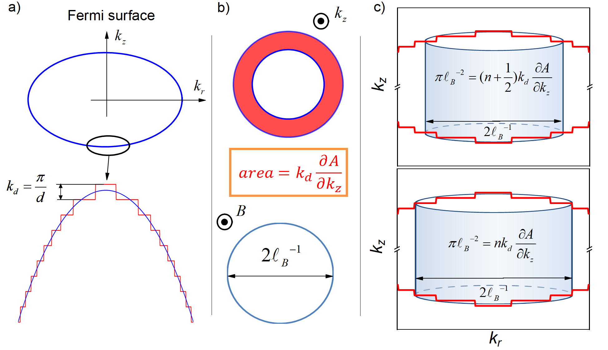
Figure 9: Steps in momentum space induced by confinement in real space. (a) Finite thickness $d$ distorts a Fermi surface. Confinement of electrons in real space modifies a smooth Fermi surface and induces steps with a height of $k_{d}=\frac{\pi}{d}$ along $k_{z}$ (red line) emerge, provided that the disorder is sufficiently small to make the wave-vector well-defined at the scale of $d^{-1}$. (b) Projected along the $k_{z}$ orientation, each step on the Fermi surface generates a flat toroid. It consists of electronic states sharing identical $k_{z}$. The area of each flat ring is $k_{d}\partial A/\partial k_{z}$. The inverse of magnetic length, $\ell_{B}^{-1}$, can become commensurate with these flat rings.(c) When the area of the lowest Landau tube (in blue) is the area of the flat ring times a half-integer (top), the electronic states (in red) condensing to the Landau level share a common $k_{z}$. When it is an integer times the area of the flat ring (bottom), these electronic states (in red) have two out-of-plane wave vectors, which differ by 2 $k_{d}$.

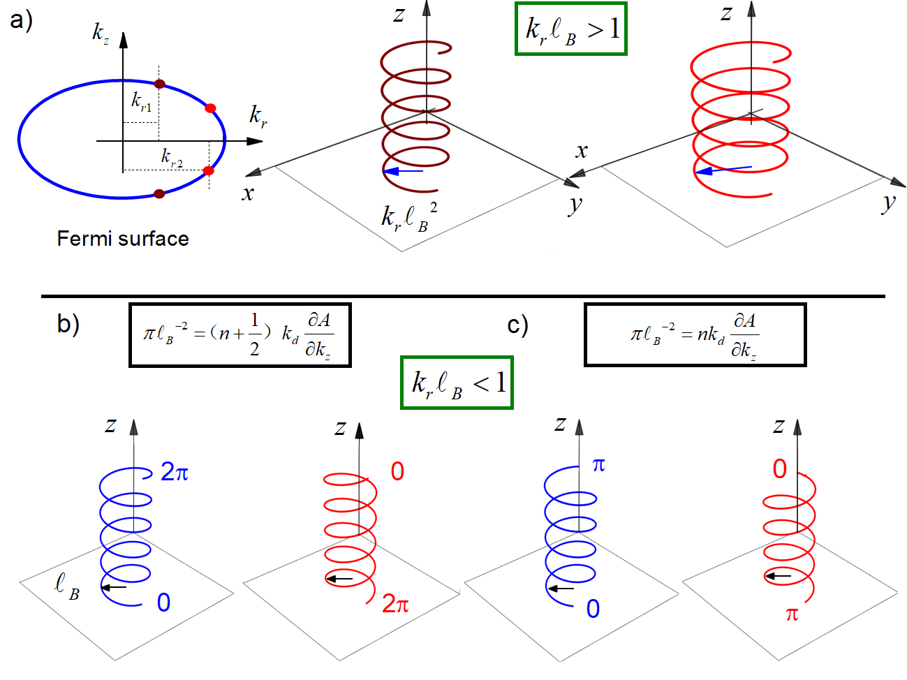
Figure 10: Helical states. (a) In the classical regime, the radius of each turn of the helical trajectory of electrons is equal to the Larmor radius. Therefore, it is different for different electrons as a function of their radial wave-vector. It is shorter for electrons closer to the pole (in brown) than those further (in red). Since this radius cannot become shorter than the magnetic length, this picture breaks down when $k_{r}\ell_{B}<1$. This is the quantum regime shown in the lower panels, b and c. (b) When the magnetic field is equal to a half-integer times the product of $\frac{\hbar}{e}$ and $k_{d}\partial A/\partial k_{z}$, the upward and the downward propagating helical states have the same phase at the start and the end of their trajectories. The interference is expected to be constructive. (c) When the magnetic field is equal to an integer time the product of $\frac{\hbar}{e}$ and $k_{d}\partial A/\partial k_{z}$, there is $\pi$ phase shift. The interference is expected to be destructive.

III.2 A Fermi surface sculpted by spatial confinement

Confinement of electrons in real space has implications for the energy spectrum in reciprocal space, a fact established by research on quantum dots [36]. In a metallic sample of finite size, the Fermi surface ceases to be smooth. This is illustrated in Fig.9a. A finite thickness of $d$ along the $z$ direction in real space implies steps on the Fermi surface along $k_{z}$ with a height of $k_{d}=\frac{\pi}{d}$. For $k$ to remain a good quantum number at such a short scales in reciprocal space, electronic waves are to remain well-defined in real space over a length exceeding $d$. The defect limited mean free path is as long as $\sim 150\mu$m (See table 1). Therefore, at least for our thinner samples, this criterion is easily met.

Since energy and particle number are both conserved, such a reorganization of electronic states has consequences for their in-plane wave-vector. They change to keep the total volume of the Fermi surface and the total energy identical to those in an infinite sample. As illustrated in Fig.9b, each step on the Fermi surface generates a flat toroid, with an area proportional to $k_{d}\times\partial A/\partial k_{z}$. When the thickness changes from 12.5 to 100 $\mu$m, $k_{d}$ varies between $2\pi/(1.2\times 10^{5})\simeq 5\times 10^{-5}$ Å^-1 to $2\pi/(1\times 10^{6})\simeq 6\times 10^{-6}$Å^-1. We saw above, $k_{d}\times\partial A/\partial k_{z}$ does not display any detectable change even when $k_{z}$ deviates from its maximum by $0.01$Å^-1. Therefore, the $k_{d}\times\partial A/\partial k_{z}$ product, i.e. the area of each flat toroid, is constant in our range of interest ($\sim 10k_{d}$). Note that this would have not been the case in absence of linear dispersion along the out-of-plane orientation.

With a magnetic field along the $z$-axis, Landau quantization will emerge. The expression for lowest Landau level is [37]:

$$\Psi_{0}=\frac{1}{\sqrt{2\pi}\ell_{B}}{\rm{exp}}[-\frac{r^{2}}{4\ell_{B}^{2}}]$$ (6)

Here, $r=\sqrt{x^{2}+y^{2}}$ and $\ell_{B}$ is the magnetic length. This wave-function replaces the zero-field Bloch waves as the in-plane spatial distribution of the electronic states, when $\ell_{B}^{-2}\approx k_{d}\partial A/\partial k_{z}$ (Fig. 9b).

In this picture, each oscillation corresponds to an intersection between the lowest landau tube and a flat toroid. Each oscillation is an alternation between two situations depicted in Fig. 9c. The Landau tube can reside in the middle of a flat toroid, which corresponds to:

$$\pi\ell_{B}^{-2}=(n+\frac{1}{2})k_{d}\frac{\partial A}{\partial k_{z}}$$ (7)

In this case, the electronic states, which condense to the lowest Landau level all share an identical $k_{z}$.

When the Landau tube is at the boundary between two neighboring toroids, one has:

$$\pi\ell_{B}^{-2}=nk_{d}\frac{\partial A}{\partial k_{z}}$$ (8)

In this case, two neighboring flat toroids with slightly different out-of-plane wave-vectors ($\delta k_{z}=2k_{d}$) are involved.

The period of oscillations given by equations 7 and 8 is:

$$\delta(\ell_{B}^{-2})=d^{-1}\frac{\partial A}{\partial k_{z}}$$ (9)

This is identical to the semiclassical expression (Eq. 2). Thus, invoking a commensurability in momentum space in the present picture leads to a conclusion identical to the one obtained by invoking a real space commensurability [3].

The present picture, which links Sondheimer oscillations to Landau quantization, is compatible with our finding that they disappear when $T>8$K and $k_{B}T>\hbar\omega_{c}$ (See supplementary note 4 [30]). This quantized version of Sondheimer oscillations appears as a mirror image of Shubnikov-de Haas (or de Haas-van Alphen) oscillations [6]. Both occur by intersections between the Landau tubes and the Fermi surface. In one case, oscillations arise when the $n$th Landau tube intersects the extremal cross section of the Fermi surface. In the other, oscillations arise because the lowest Landau tube intersects the $n$th flat toroid of the Fermi surface. This inversion transforms a periodicity in $B^{-1}$ to a periodicity in $B$.

III.3 Quantum-classical crossover

The semi-classical picture of Sondheimer oscillations, which was recalled in the introduction, does not invoke Landau quantization. There, the Lorentz force generates helical trajectories in the real space. Oscillations arise because of the commensurability between the helix pitch and the sample thickness. Now, the radius of each helix turn is equal to the Larmor radius of electrons, set by the compensation between the Lorentz force and the centripetal force: $R=\frac{p_{\perp}}{eB}$. Here, $p_{\perp}=\hbar k_{r}$ is the in-plane momentum of the electron. Since electrons on the Fermi surface have different in-plane momenta, their Larmor radius is not identical. Let us express the latter as a function of the magnetic length:

$$R=\ell_{B}^{2}k_{r}$$ (10)

As illustrated in Fig. 10a, at a given magnetic field, electronic helical trajectories have different radii (but the same pitch). The smaller, the radial wave-vector of an electron, the shorter would be its Larmor radius. But, this picture cannot remain indefinitely valid. Since the Larmor radius cannot become shorter than the magnetic length, the classical picture is expected to break down for states so close to the pole, such that $k_{r}\ell_{B}<1$. The quantum picture, drawn in the previous section is relevant for these states, because of this lower boundary to the helix radius set by the magnetic length. In the quantum regime, the helical trajectories in real space are quantized. They consist of one-dimensional states, which are localized in the plane but have finite kinetic energy in the perpendicular orientation. These quantum helices share the same pitch (and hence the same periodicity) of their classical counterpart. In contrast, they share identical radii ($\ell_{B}$) too.

The generic field dependence of the classical Sondheimer oscillations is $\propto B^{-4}$ (See equation 5). Bulk magnetoconductivity follows $B^{-2}$. The additional exponent (of -2) is due to field-induced shift in the relative weight of the electronic states. Those with smaller $k_{r}$ have a shorter Larmor radius. Because of the replacement of $\ell_{B}^{2}k_{r}$ with $\ell_{B}$, one expects the quantum version of oscillations to have a milder decay with magnetic field and in equation 4, it is indeed $\propto B^{-2.5}$.

As seen in the supplementary note 3, the high-field oscillations do not display a scaling as perfect as the one seen for low-field (quantized) oscillations. However, our data confirms that the thickness dependence of the two types of oscillations is different, as implied by the contrast between Eq. 5 and Eq. 4. The quantized oscillations dominate at low field and thin crystals as a consequence of their milder decay with field and thickness.

III.4 Quantum corrections and tunneling

A rigorous account of transport in the quantum regime is missing. Let us, however, show that the quantum scenario can lead to a sinusoidal oscillation between positive and negative corrections to magneto-conductivity as well as to an exponential term.

As seen in Fig. 8, the oscillations consist of an alternation between positive and negative corrections to the total magnetoconductance. When the magnetic field times thickness is an integer (half-integer) times $\frac{\hbar}{e}\partial A/\partial k_{z}$, i.e. when Equation 8 (7) holds, the correction is positive (negative). This indicates a succession of constructive and destructive interference between phase coherent quantum states.

Electronic states with $k_{r}<\ell_{B}^{-1}$ acquire $\Psi_{0}$ as their in-plane wave-function, while remaining Bloch waves along the magnetic field. The combination gives rise to helical states with a well-defined amplitude and phase. When the commensurability is half-integer, all these electronic states share an identical $k_{z}=m\times k_{d}$, where $m$ is an integer. The phase shift between the bottom and the top boundaries is $2\pi\times m$. In real space, there are two helices each associated with one orientation of $k_{z}$ (Fig. 10b). In contrast, when the commensurability is integer, the existence of two slightly different out-of-plane wave-vectors ($k_{z1}=m\times k_{d}$ and $k_{z2}=(m-2)\times k_{d}$ ) leads to $k_{z}=(m-1)\times k_{d}$ and a phase shift between the bottom and the top boundaries equal to $m\times\pi$. In this case, each helical state has a phase shift of $\pi$ between its two extremities (Fig. 10c). The contrast between the two configurations provides a route towards alternating constructive and destructive interference as the source of positive and negative corrections to magneto-conductivity.

Quantum tunneling is the most plausible source of $e^{-B/B_{0}}$ term in the expression for in-plane conductivity. The helical states constructed from the electronic states with $k_{r}<\ell_{B}^{-1}$ are distinct from the Fermi sea (the remaining electrons for which $k_{r}>\ell_{B}^{-1}$) and harboring unquantized helices. Tunneling is poorly understood for dimensions larger than one [35, 38]. In general, however, it leads to a probability of $e^{-s/\hbar}$, where $s$ is the tunneling action [35]. Experimentally, we find that that $B_{0}\simeq 3\Delta B$. In the tunneling scenario, this would lead to a tunneling action of:

$$s\simeq e\frac{B}{k_{d}\partial A/\partial k_{z}}$$ (11)

Thus, the relevant action would be the product of the charge of the electron (the particles of the Fermi Sea) and the magnetic flux in a flat toroid (the fundamental bricks of the quantized helical states).

IV Conclusion

In summary, we showed that in thin single crystals of cadmium hosting ballistic electrons, magnetomorphic (known as Sondheimer) oscillations display a field dependence never encountered before. They consist of a succession of negative and positive corrections to the total magnetoconductance. Their amplitude is set by the quantum of conductance multiplied by a coefficient, which depends uniquely on the sample thickness and the Fermi surface geometry. We argued that to explain this experimental observation, one needs to go beyond the available semi-classical theories and formulate a quantum theory taking into account the formation of steps and flat toroids on the Fermi surface and their interplay with Landau quantization. We argued that the classical theory of Sondheimer oscillations is expected to break down when the Larmor radius becomes as short as the magnetic length, which is the case for states with a small radial wave-vector.

The semi-Dirac dispersion of the conduction band [34] plays a key role in this physics. It generates a well-defined length scale of $\partial A/\partial k_{z}$ in reciprocal space over a significant slice of $k_{z}$. Quantum effects associated with the lowest Landau level emerge when $\ell_{B}^{2}d^{-1}\partial A/\partial k_{z}\simeq 1$. This is to be contrasted with the so-called extreme quantum limit, which requires $\ell_{B}k_{F}\simeq 1$, and is encountered in dilute metals [39, 40, 41, 42].

Finally, let us note that the quantum limit of Sondheimer oscillations is yet another manifestation of an Aharaonv-Bohm (AB) flux through a closed path [43]. Such a universality is known given the relevance of AB physics to Altshuler, Aranov, and Spivak oscillations [44, 45] and to the Quantum Hall Effect [46], following Laughlin’s argument [47]. In all these cases, flux quantization occurs even in absence of a simple well-defined loop in real space.

V Acknowledgments

We thank Benoît Fauqué and Alaska Subedi for discussions. This work is part of a Cai Yuanpei Franco-Chinese collaboration program (No. 51258NK). In China, it was supported by the National Science Foundation of China (Grant No. 12474043, 12004123 and 51861135104), the National Key Research and Development Program of China (Grant No. 2022YFA1403500), and the Fundamental Research Funds for the Central Universities (Grant no. 2019kfyXMBZ071). X. L. was supported by the National Key Research and Development Program of China (Grant No.2023YFA1609600) and the National Science Foundation of China (Grant No. 12304065). We also acknowledge a grant from the Île de France region.

Supplementary Materials for “Quantization of Sondheimer oscillations of conductivity in thin cadmium crystals”

Note 1. Materials and Methods.

Sample growth. Cd single crystals were grown by the vapor-phase transport method. A quartz tube with appropriate amounts of starting material Cd (99.9997%) was kept at the growth temperature for two weeks in a two-zone furnace. Shiny plate-like crystals were produced in a temperature gradient of 300 –200^∘C.

Fabrication of the samples. The production method followed previous works [17]. First, the crystallographic orientation of the bulk crystal was determined using X-ray diffraction. Subsequently, the crystal was securely affixed to a SEM stub in the desired orientation. The critical step was to employ a focused beam of Ga ions to meticulously carve a rectangular slab, a lamella, from the crystal. This process unfolds in three stages.

Initially, a high current of 50 nA was used to create two gaps within the crystal. These gaps were separated by a section of the crystal, approximately $\sim$25 $\mu$m thick and 150 $\mu$m long. Following this, a smaller current of 15 nA was applied to smoothen the crystal section, resulting in moderately flat sidewalls. The lamella remained attached to the parent crystal through two beams at its top.

Afterwards, with a precise 7 nA current both sides of the lamella were fine cut, ensuring parallel sidewalls and a high level of smoothness. The obtained flakes were then carefully transferred to an alumina substrate. It is crucial to note that a very thin layer of “Araldite” epoxy adhesive must be applied to the substrate beforehand. Once positioned atop the epoxy adhesive, capillary forces naturally shaped the epoxy around the lamella, extending smoothly to each of its top surfaces without covering them.

After allowing the epoxy adhesive to dry naturally, the substrate was taken to a sputtering machine. There, a brief RF etching process was performed, depositing a 300 nm layer of Au onto the lamella. To further refine the device, the Scios 2 system was utilized. Initially, the Au layer covering the active part of the device was removed using an acceleration voltage of 5 kV and an ion current of 2 nA. Subsequently, the overall device shape, including the contact positions, was precisely cut out at 0.3 nA and 30 kV. Finally, the Au layer away from the device was severed, ensuring a current flow exclusively through the device. With these steps completed, the device become ready for measurement.

Note 2. Magneto-morphic oscillations in samples with the thickness between 100$\mu$m to 475$\mu$m .

Fig. S1 shows magneto-morphic oscillations of longitudinal and transverse electrical resistivity in the $d$ = 100 $\mu$m-thick cadmium single crystal at 2 K. Due to the quadratic dependence of orbital magnetoresistance on the magnetic field, the longitudinal resistivity was dominated by a large background. The Sondheimer oscillations are clearly visible in the Hall signal, where the background is smaller as a result of compensation between electrons and holes.

By inverting the measured resistivity tensor, we quantified the conductivity tensor, using $\sigma_{ij}=\frac{-\rho_{ij}}{\rho_{ii}^{2}+\rho_{ij}^{2}}$. As a result, when the field is less than $B_{1}$, the longitudinal and transverse conductivity fall off as $B^{-2.5}$$e^{-B/3\Delta B}$, as shown in Fig.S1c and d. When the field is greater than $B_{1}$, the amplitude decay follows $B^{-4}$.

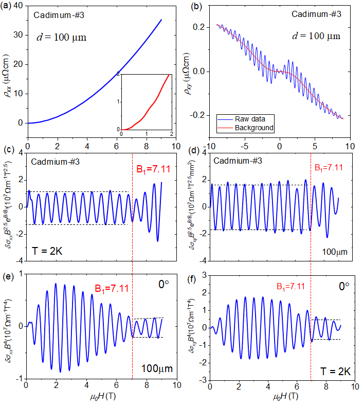
Figure S1: Magneto-morphic oscillations in 100$\mu m$ sample. (a) Longitudinal resistivity at 2 K. (b) Transverse resistivity at 2K. (c),(d) Longitudinal and transverse conductivity fall off $\propto B^{-2.5}e^{-B/B_{0}}$ when the field is less than $B_{1}$ in the 100 $\mu m$ sample. (e),(f) Longitudinal and transverse conductivity fall off $\propto B^{-4}e^{-B/B_{0}}$ when the field is greater than $B_{1}$.

Furthermore, longitudinal and transverse electrical resistivity of the $d$ = 200 $\mu$m cadmium micro-ribbons at 2 K is shown in Fig.S2. Oscillations are observed in the Hall signal with period about $\sim$ 0.28 T. When the field is less than $B_{1}$, the amplitude of oscillation fall off as $\propto B^{-2.5}e^{-B/3\Delta B}$ shown in Fig.S2e and f.

Longitudinal and transverse electrical resistivity of the $d=$ 475$\mu$m cadmium sample are also shown in Fig.S3. The evident magneto-morphic oscillations is observed in the Hall signals with period about $\sim$ 0.12 T. When the field is less than $B_{1}$, the amplitude of oscillation fall off as $\propto B^{-2.5}e^{-B/3\Delta B}$ as shown in Fig.S3.

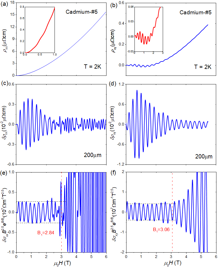
Figure S2: Magneto-morphic oscillations in the 200 $\mu$m sample. (a) Longitudinal resistivity at 2 K. (b) Transverse resistivity at 2 K. Oscillations at low field are shown in the insert. (c),(d) The amplitude of SO for longitudinal and transverse resistivity in 200 $\mu$m sample. (e) The longitudinal conductivity fall off as $\propto B^{-2.5}e^{-B/3\Delta B}$ when the field is less than $B_{1}$. (f) Transverse conductivity fellow as $\propto B^{-2.5}e^{-B/3\Delta B}$ when the field is less than $B_{1}$.

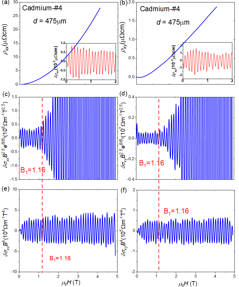
Figure S3: Magneto-morphic oscillations in 475$\mu$m sample. (a) Longitudinal resistivity at 2K. (b) Transverse resistivity at 2K. The evident magneto-morphic oscillations is observed in the low field as shown in insert. (c),(d) Longitudinal and transverse conductivity fall off as $\propto B^{-2.5}e^{-B/3\Delta B}$ when the field is less than $B_{1}$. (e),(f) Longitudinal and transverse conductivity fall off as $\propto B^{-4}$ when the field is greater than $B_{1}$.

Note 3. The field and thickness dependence of oscillations in the two regimes

As the sample becomes thicker, the $B_{1}$ threshold field separating the two types of amplitude field dependence shifts downward. We subtracted the amplitude of oscillations in both two regions. They are shown in Fig.S4. When the field is less than $B_{1}$, the oscillation fall off as $B^{-2.5}e^{-3B/\Delta B}$. The longitudinal and the transverse conductivity are shown in Fig.S4a and c, respectively. However, when the field is greater than $B_{1}$, the oscillations decay by $B^{-4}$. A similar behavior was observed for longitudinal and transverse conductivity, as seen in Fig.S4b and d.

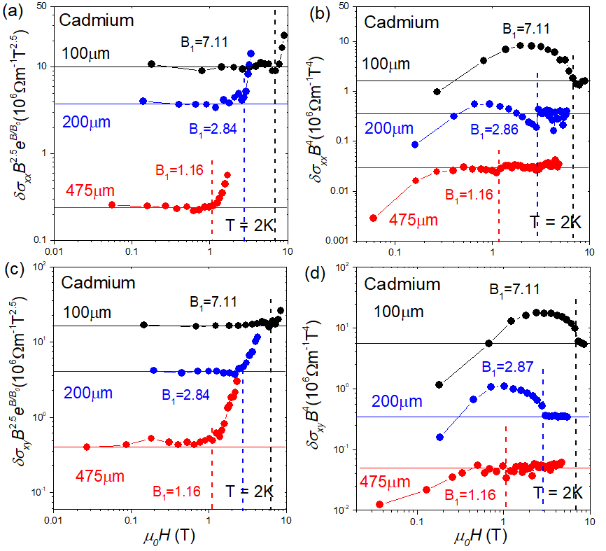
Figure S4: The field dependence of oscillation amplitude. (a), (b) For longitudinal conductivity, when the field is less than $B_{1}$, the SO oscillation can be expressed as $\delta\sigma_{xx}\propto B^{-2.5}e^{-B/B_{0}}$. At the higher field, the SO oscillation is dominated by the $B^{-4}$. (c), (d) In Hall conductivity, the same result is obtained.

When the field is less than $B_{1}$, the amplitude falls off as $\propto B^{-2.5}e^{B/3\Delta B}$. Multiplying the amplitude of oscillations by $d^{2}$ and plotting $\delta\sigma_{ij}B^{2.5}d^{2}$ leads to Fig.S5. All curves fall on top of each other.

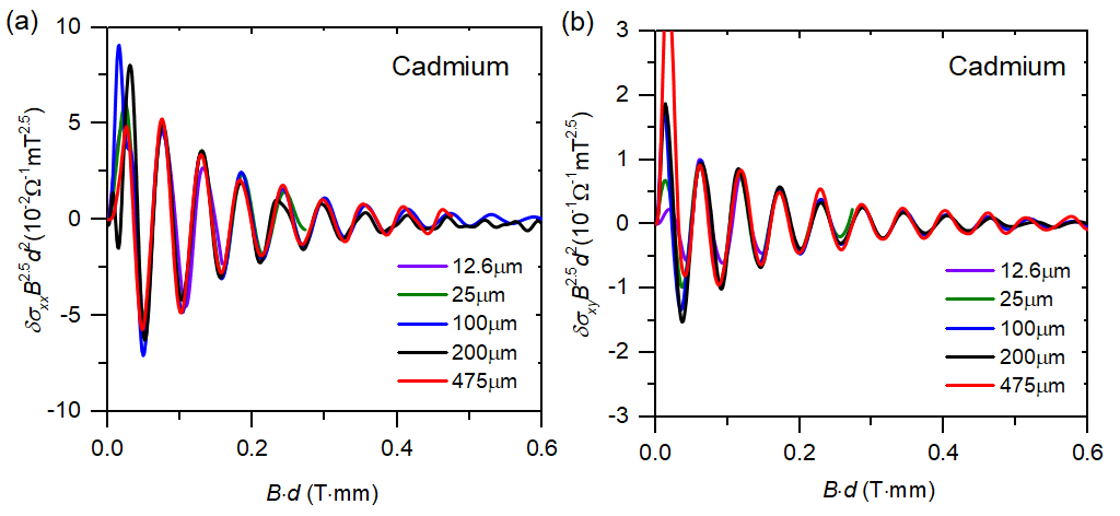
Figure S5: Scaling of the low-field ($B<B_{1}$) oscillations with thickness. (a) Amplitude of $\sigma_{xx}$ oscillation multiplied by $d^{2}$ as a function of the product of field and thickness. All curves collapse. (b) Same or the Hall conductivity $\sigma_{xy}$.

When the field is larger than $B_{1}$, the amplitude falls off as $\propto B^{-4}$. Multiplying the amplitude of oscillations by $d^{3}$ and plotting $\delta\sigma_{ij}G_{0}^{-1}\ell_{B}^{-8}d^{3}$ leads to Fig.S6. The scaling is not as good as in the case of low-field ($B<B_{1}$) oscillations. Nevertheless, we found that $d^{-3}$ is a much better scaling than $d^{-2}$ and $d^{-4}$.

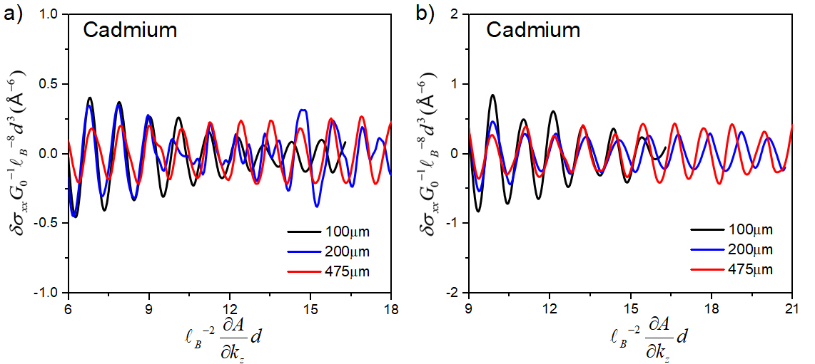
Figure S6: Variation of high-field oscillations with field and with thickness. (a) The vertical axis in conductivity divided by the quantum of conductance $G_{0}$ and multiplied by $\ell_{B}^{-8}\times d^{3}$. The horizontal axis is linear in magnetic field. (b) Same for the Hall conductivity $\sigma_{xy}$.

Note 4. The temperature dependence of the oscillations in 25 $\mu$m sample.

We investigated the temperature dependence of resistivity in the 25 $\mu$m cadmium sample. As shown in Fig.S7, magneto-morphic oscillations in longitudinal and Hall resistivity weaken with warming. The evolution of $\delta\sigma_{xy}B^{2.5}e^{B/B_{0}}$ with temperature is show in Fig.S7c. Oscillations remain sinusoidal at different temperatures. As seen in Fig.S7d, the amplitude of the oscillations decrease linearly with rising temperature and they disappear totally when $T\simeq$ 8.5 K.

Taking the computed in-plane mass of the electron pocket $m_{\perp}=0.8m_{0}$ [34], one finds that the cyclotron energy at 10 T is about 7 K. Thus, the disappearance of these oscillations is concomitant with the $k_{B}T\sim\hbar\omega_{c}$ boundary.

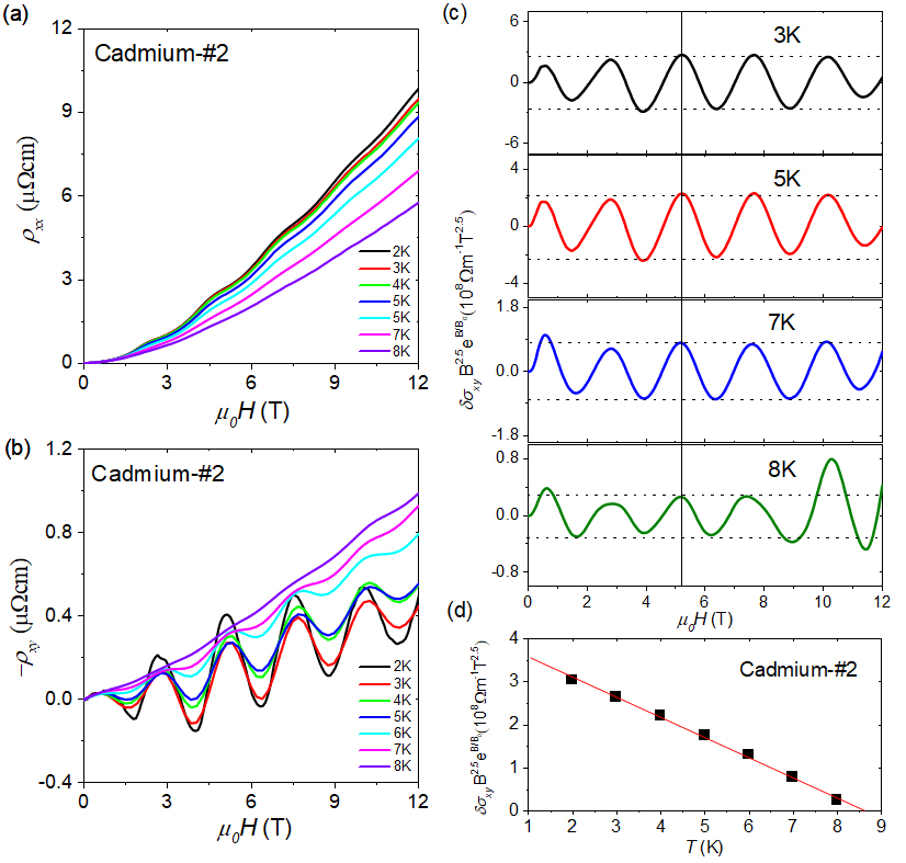
Figure S7: Temperature dependence of magneto-morphic oscillation in 25 $\mu$m sample. (a) Temperature dependence of longitudinal resistivity $\rho_{xx}$ in 25 $\mu$m sample. (b) Temperature dependence of transverse resistivity $\rho_{xy}$ in 25 $\mu$m sample. (c) Temperature dependence of $\delta\sigma_{xy}B^{2.5}e^{B/B_{0}}$ in 25 $\mu$m sample. A sinusoidal oscillation is obtained in different temperatures. (d) The amplitude of the third oscillation marked by the black line in (c) as a function of temperature.

References

- Sondheimer [1952] E. H. Sondheimer, The mean free path of electrons in metals, Advances in Physics 1, 1 (1952).
- Brändli and Olsen [1969] G. Brändli and J. Olsen, Size effects in electron transport in metals, Materials Science and Engineering 4, 61 (1969).
- Chambers [1971] R. Chambers, The physics of metals. 1. Electrons, edited by J. Ziman, vol. 1 (Cambridge University Press, 1971).
- Trivedi and Ashcroft [1988] N. Trivedi and N. W. Ashcroft, Quantum size effects in transport properties of metallic films, Phys. Rev. B 38, 12298 (1988).
- Sondheimer [1950] E. H. Sondheimer, The influence of a transverse magnetic field on the conductivity of thin metallic films, Phys. Rev. 80, 401 (1950).
- Shoenberg [1984] D. Shoenberg, Magnetic Oscillations in Metals, Cambridge Monographs on Physics (Cambridge University Press, 1984).
- Hurd [2012] C. Hurd, The Hall effect in metals and alloys (Springer Science & Business Media, 2012).
- Grenier et al. [1966] C. G. Grenier, K. R. Efferson, and J. M. Reynolds, Magnetic field dependence of the size effect in the transport coefficients of a cadmium single crystal at liquid-helium temperatures, Phys. Rev. 143, 406 (1966).
- Alstadheim and Risnes [1968] T. Alstadheim and R. Risnes, Sondheimer oscillations in aluminium single crystals, Philosophical Magazine 18, 885 (1968).
- Sato [1979] H. Sato, Sondheimer oscillation in aluminium single crystals, physica status solidi (b) 94, 309 (1979).
- Hambourger and Marcus [1973] P. D. Hambourger and J. A. Marcus, Size-dependent oscillatory magnetoresistance in cadmium, Phys. Rev. B 8, 5567 (1973).
- Mackey et al. [1970a] H. J. Mackey, J. R. Sybert, and R. D. Hight, Magnetomorphic oscillations in the electrical conductivity of cadmium cylinders, Phys. Rev. B 1, 2385 (1970a).
- Mackey et al. [1970b] H. J. Mackey, J. R. Sybert, and W. M. Waller, Observations of magnetomorphic oscillations in Zn and Cd by a modified field-modulation technique, Phys. Rev. B 1, 3979 (1970b).
- Trodahl [1971] H. J. Trodahl, The Sondheimer size effect in indium single crystals, Journal of Physics C: Solid State Physics 4, 1764 (1971).
- Sakamoto [1976] I. Sakamoto, Galvanomagnetic size effect in copper, Journal of the Physical Society of Japan 41, 1317 (1976).
- Munarin et al. [1968] J. A. Munarin, J. A. Marcus, and P. E. Bloomfield, Size-dependent oscillatory magnetoresistance effect in gallium, Phys. Rev. 172, 718 (1968).
- Van Delft et al. [2021] M. R. Van Delft, Y. Wang, C. Putzke, J. Oswald, G. Varnavides, C. A. Garcia, C. Guo, H. Schmid, V. Süss, H. Borrmann, et al., Sondheimer oscillations as a probe of non-ohmic flow in crystals, Nature communications 12, 4799 (2021).
- Taen et al. [2023] T. Taen, A. Kiswandhi, and T. Osada, Magnetic-field periodic quantum Sondheimer oscillations in thin-film graphite, Phys. Rev. B 108, 235411 (2023).
- Harrison [1960] W. A. Harrison, Electronic structure of polyvalent metals, Phys. Rev. 118, 1190 (1960).
- Tellier [1989] C. Tellier, A two-band model for the galvanomagnetic properties of thin semimetal films, Journal of materials science 24, 2309 (1989).
- Katyal and Gerritsen [1969] O. P. Katyal and A. N. Gerritsen, Investigation of Hall resistivity and magnetoresistance of cadmium and cadmium-zinc crystals, Phys. Rev. 178, 1037 (1969).
- Hambourger et al. [1967] P. Hambourger, J. Marcus, and J. Munarin, Size dependent oscillatory magnetoresistance in cadmium, Physics Letters A 25, 461 (1967).
- Zebouni et al. [1963a] N. H. Zebouni, R. E. Hamburg, and H. J. Mackey, Magnetomorphic oscillations in the Hall effect and magnetoresistance in cadmium, Phys. Rev. Lett. 11, 260 (1963a).
- Tsui and Stark [1966] D. C. Tsui and R. W. Stark, de Haas-van Alphen effect, magnetic breakdown, and the Fermi surface of cadmium, Phys. Rev. Lett. 16, 19 (1966).
- Zebouni et al. [1963b] N. H. Zebouni, R. E. Hamburg, and H. J. Mackey, Magnetomorphic oscillations in the Hall effect and magnetoresistance in cadmium, Phys. Rev. Lett. 11, 260 (1963b).
- Mackey et al. [1967] H. J. Mackey, J. R. Sybert, and J. T. Fielder, Effect of sample geometry on magnetomorphic oscillations in the hall effect in cadmium at liquid-helium temperatures, Phys. Rev. 157, 578 (1967).
- Gurevich [1959] V. Gurevich, Oscillations in the conductivity of metallic films in magnetic field, Sov. Phys. JETP 35, 464 (1959).
- Chambers [1969] R. Chambers, Transport properties: surface and size effects, The Physics of Metals 1 (1969).
- Moll [2018] P. J. Moll, Focused ion beam microstructuring of quantum matter, Annual Review of Condensed Matter Physics 9, 147 (2018).
- SM [2024] See the Supplemental Material (2024).
- Zhu et al. [2018] Z. Zhu, B. Fauqué, K. Behnia, and Y. Fuseya, Magnetoresistance and valley degree of freedom in bulk bismuth, Journal of Physics: Condensed Matter 30, 313001 (2018).
- Fauqué et al. [2018] B. Fauqué, X. Yang, W. Tabis, M. Shen, Z. Zhu, C. Proust, Y. Fuseya, and K. Behnia, Magnetoresistance of semimetals: The case of antimony, Phys. Rev. Mater. 2, 114201 (2018).
- Pippard [1989] A. Pippard, Magnetoresistance in Metals, Cambridge Studies in Low Temperature Physics (Cambridge University Press, 1989).
- Subedi and Behnia [2024] A. Subedi and K. Behnia, Semi-dirac fermions in hexagonal close-packed cadmium (2024), arXiv:2411.11585 [cond-mat.mtrl-sci] .
- Wilkinson [1986] M. Wilkinson, Tunnelling between tori in phase space, Physica D: Nonlinear Phenomena 21, 341 (1986).
- Alivisatos [1996] A. P. Alivisatos, Semiconductor clusters, nanocrystals, and quantum dots, Science 271, 933 (1996).
- Yoshioka [2002] D. Yoshioka, The Quantum Hall Effect, Physics and astronomy online library (Springer, 2002).
- Creagh [1998] S. C. Creagh, Tunnelling in two dimensions, in Tunneling in Complex Systems (World Scientific, 1998) pp. 35–100.
- Fauqué et al. [2013] B. Fauqué, D. LeBoeuf, B. Vignolle, M. Nardone, C. Proust, and K. Behnia, Two phase transitions induced by a magnetic field in graphite, Phys. Rev. Lett. 110, 266601 (2013).
- Zhu et al. [2017] Z. Zhu, J. Wang, H. Zuo, B. Fauqué, R. D. McDonald, Y. Fuseya, and K. Behnia, Emptying Dirac valleys in bismuth using high magnetic fields, Nature Communications 8, 15297 (2017).
- Galeski et al. [2022] S. Galeski, H. F. Legg, R. Wawrzyńczak, T. Förster, S. Zherlitsyn, D. Gorbunov, M. Uhlarz, P. M. Lozano, Q. Li, G. D. Gu, C. Felser, J. Wosnitza, T. Meng, and J. Gooth, Signatures of a magnetic-field-induced lifshitz transition in the ultra-quantum limit of the topological semimetal , Nature Communications 13, 7418 (2022).
- Pan and Shindou [2019] Z. Pan and R. Shindou, Ground-state atlas of a three-dimensional semimetal in the quantum limit, Phys. Rev. B 100, 165124 (2019).
- Aharonov and Bohm [1959] Y. Aharonov and D. Bohm, Significance of electromagnetic potentials in the quantum theory, Phys. Rev. 115, 485 (1959).
- Al’tshuler et al. [1981] B. L. Al’tshuler, A. G. Aronov, and B. Z. Spivak, The aaronov-bohm effect in disordered conductors, JETP Letters 33, 94 (1981).
- Pannetier et al. [1984] B. Pannetier, J. Chaussy, R. Rammal, and P. Gandit, Magnetic flux quantization in the weak-localization regime of a nonsuperconducting metal, Phys. Rev. Lett. 53, 718 (1984).
- Douçot [2011] B. Douçot, Introduction to the theory of the integer quantum Hall effect, Comptes Rendus Physique 12, 323 (2011), quantum Hall Effect and Metrology.
- Laughlin [1981] R. B. Laughlin, Quantized Hall conductivity in two dimensions, Phys. Rev. B 23, 5632 (1981).