Universal solution to the Schrieffer-Wolff Transformation Generator

Abstract

The Schrieffer-Wolff transformation (SWT) is an important perturbative method in quantum mechanics used to simplify Hamiltonians by decoupling low- and high-energy subspaces. Existing methods for implementing the SWT often lack general applicability to arbitrary perturbative systems or fail to provide a closed-form solution for the SWT generator. In this article, we present a systematic and unified framework for the SWT that addresses these shortcomings. Specifically, we derive a closed-form solution for the SWT generator that is universally applicable to any system that satisfies the conditions required to be perturbatively treated. Furthermore, we extend this solution to time-dependent systems with periodic perturbations, covering all frequency regimes. The effectiveness of this approach is then demonstrated by applying it to analyze the dispersive shift of an anharmonic resonator coupled to a two-level system with time-dependent coupling.

I Introduction

The Schrieffer-Wolff transformation (SWT) is a widely utilized perturbation theory approach for simplifying the analysis of complex quantum systems. Unlike traditional time-independent perturbation theory, which focuses on computing corrections to the energy levels of a system, the SWT transforms the original Hamiltonian into an effective low-energy Hamiltonian by eliminating interactions between disparate energy subspaces. This makes the SWT particularly advantageous for studying problems in condensed matter physics Villarreal et al. (2022); Kale et al. (2022); Voleti et al. (2021); Hu et al. (2023); Manning-Coe and Bradlyn (2023); Kolley and Kolley (1990); Hörmann and Schmidt (2023); Lovtsov and Yu. Yushankhai (1991); Sun et al. (2021); Weisse et al. (2024), quantum optics Allard and Weick (2023); Jäger et al. (2022); Solgun et al. (2019); Pelegrí et al. (2024); Shani et al. (2022), quantum information sciences Kawakami et al. (2023); Hetényi et al. (2022); Mutter and Burkard (2021); Ansari (2019); Mutter and Burkard (2020); Benito et al. (2019); Wang et al. (2021); Liu et al. (2022); Zhang (2023); Cayao et al. (2020); Bosco et al. (2021); Bosco and Loss (2022); Del Vecchio and Moutanabbir (2023); Haq et al. (2022); Dey and Schliemann (2024a); Zhang et al. (2022); Marécat et al. (2023); Seedhouse et al. (2021); Hillmann and Quijandría (2022); Kowalski and Bauman (2022); Fang et al. (2023); Dey and Schliemann (2024b); Consani and Warburton (2020); Wang et al. (2023a) as well as several other fields Kessler (2012); von Witte et al. (2024); Massarelli et al. (2022); Starkov et al. (2023); Aramthottil et al. (2022), where the primary interest lies in understanding the low-energy behavior of the studied systems.

One of the key reasons for employing the SWT over other methods of perturbation theory is its ability to retain the operator structure of the Hamiltonian, thereby providing a more physical understanding of how perturbations affect the system. This contrasts with traditional approaches that mainly yield shifts to the original energy levels. It is also well known that upon second order, the SWT returns the results obtained by regular perturbation theory approaches. Additionally, slight alterations of the generally accepted SWT Magesan and Gambetta (2020), seem to suggest that this equivalence could be extended to higher orders for a variety of systems.

The implementation of the SWT has been approached through a variety of methods Kehrein and Mielke (1996); Salomaa (1988); Lee et al. (2017); Malekakhlagh et al. (2020); Tzen Ong and Jones (2011); Wurtz et al. (2020); Thomas et al. (2009); Li et al. (2022), most of which aim to construct a generator for the unitary transformation that decouples the high-energy and low-energy subspaces of a given Hamiltonian. These methods can broadly be categorized into two classes: operator-level approaches and matrix-element-based approaches. In the operator approach, originally introduced by Schrieffer and Wolff Schrieffer and Wolff (1966), the generator is typically found by solving an operator equation that relates the unperturbed Hamiltonian to the perturbation. This method preserves the operator structure, thus offering valuable physical insights. However, this often relies on heuristic assumptions that make it difficult to generalize: this is especially true for infinite-dimensional systems where determining the generator can be particularly challenging.

In contrast, matrix-element-based approaches systematically sum over the interactions between the states of the system, providing a more procedural and straightforward path to deriving the effective Hamiltonian. However, these approaches sacrifice some of the intuitive understanding provided by the operator methods, as the focus shifts from the operator-level dynamics to the energy levels. Moreover, matrix-element methods encounter significant difficulties when dealing with infinite-dimensional Hilbert spaces, as they inherently require truncation of these spaces, which compromises their ability to accurately capture the system’s dynamics.

Despite the extensive literature on the SWT, most existing methods fail to provide a close-form solution that is applicable to any system. Rather, they tend to offer reformulations that simplify the process of finding the generator in specific cases, without addressing the need for a universally applicable solution. One notable exception is the work presented in Kim et al. (2021), where the authors offer a general solution to the SWT generator that is applicable to a broad class of systems. However, their approach is limited to time independent systems with either purely bosonic or purely fermionic Hilbert spaces and does not account for interactions between finite and infinite-dimensional subspaces.

The primary objective of this article is to overcome the limitations of current SWT implementations by presenting a universal solution for the SWT generator that can be applied to any perturbative system. To achieve this, we propose a unified framework that integrates the operator and matrix-element approaches into a cohesive methodology. This approach enables the construction of effective Hamiltonians while preserving operator-level insights, eliminating the need for heuristic assumptions or truncation of the total Hilbert space. Additionally, we extend the this solution to time-dependent systems, offering a universal formalism applicable to a wide range of scenarios encountered in the study of quantum systems.

II Framework

II.1 The Schrieffer-Wolff Transformation

In this section we provide an introduction to the most widely accepted description of the SWT Winkler (2003). Due to the large amount of literature covering the topic, we here provide only those details required to understand our main results.

Consider a system described by a Hamiltonian $\mathcal{H}$ that can be partitioned into two parts

$$\mathcal{H}=\sum_{i=0}\mathcal{H}^{(i)}+\sum_{j=1}V^{(j)},$$ (1)

where $\mathcal{H}^{(0)}$ represents the unperturbed Hamiltonian of the system, whose solutions are known. Therefore, $\mathcal{H}^{(0)}$ is assumed to have a spectrum of eigenstates $\{\ket{n}\}$, associated with energies $\{E_{n}\}$, which are here assumed to contain a low-energy susbpace (spanned by states $\{\ket{L}\}$) and a high-energy subspace (spanned by $\{|H\rangle\}$). These are then coupled to eachother via the perturbative interaction terms $V^{(j)}$ of order $j$. The remaining $\mathcal{H}^{(i)}$ terms in Eq. (1) can then be interpreted as the diagonal blocks defining the preturbative dynamics of order $i$, within the $\{\ket{L}\}$ and $\{\ket{H}\}$ subspaces. The objective of the standard SWT is to construct an effective Hamiltonian $\mathcal{H}_{\text{eff}}$ that acts only within the low-energy subspace, encapsulating the influence of the high-energy states without explicitly involving them.

The transformation is constructed via a unitary operator $U=e^{-S}$, where $S$ is an anti-Hermitian operator, $S^{\dagger}=-S$, chosen to eliminate the coupling between the $\{|L\rangle\}$ and $\{|H\rangle\}$ subspaces to desired order in the perturbation $\sum_{j}V^{(j)}$. The transformed Hamiltonian is expressed as

$$\mathcal{H}_{\text{eff}}=U\mathcal{H}U^{\dagger}=e^{-S}\mathcal{H}e^{S}.$$ (2)

Using the Baker-Campbell-Haussdorf formula we expand the exponential as the series

$$\mathcal{H}_{\text{eff}}=\mathcal{H}+[\mathcal{H},S]+\frac{1}{2}[[\mathcal{H},S],S]+\cdots.$$ (3)

As stated, the goal is to then choose $S$ such that the block off-diagonal coupling between the the $\{|L\rangle\}$ and $\{|H\rangle\}$ subspaces vanishes up to desired order. It is then necessary to split the unitary generator into its perturbation series $S=\sum_{j=1}S^{(j)}$. With this we perform a second order transformation by writing

$$\mathcal{H}_{\text{eff}}\approx \sum_{i=0}^{2}\mathcal{H}^{(i)}+\sum_{j=1}^{2}V^{(j)}+$$

$$+[\mathcal{H}^{(0)},S^{(1)}]+[\mathcal{H}^{(0)},S^{(2)}]+[\mathcal{H}^{(1)},S^{(1)}]+$$

$$+[V^{(1)},S^{(1)}]+\frac{1}{2}[[\mathcal{H}^{(0)},S^{(1)}],S^{(1)}].$$ (4)

Equation (4) provides the necessary conditions for a block-diagonalization of $\mathcal{H}$ up to second order. These are then usually established in two mathematically equivalent ways. The first is to work on a operator level and solve the operator equations

$$[\mathcal{H}^{(0)},S^{(1)}] =-V^{(1)}\equiv P^{(1)},$$ (5)

$$[\mathcal{H}^{(0)},S^{(2)}] =-V^{(2)}-[\mathcal{H}^{(1)},S^{(1)}]\equiv P^{(2)}.$$ (6)

These equations are often solved via heuristic approaches by first guessing the form of $S^{(j)}$ based on the form of the perturbation $P^{(j)}$. This method allows us to retain the operator character of the SWT approach; however, for complicated perturbations, guessing the correct form of $S^{(j)}$ is often too difficult of a task.

The second method usually adapted for solving for $S^{(j)}$ is to relate it to the inverse energy difference between the low and high-energy states, effectively capturing the perturbative nature of the interaction. This is often achieved by considering the matrix elements $\bra{L}S^{(j)}\ket{H}$ of $S^{(j)}$. Explicitly, for a small perturbation of order $j$, $S^{(j)}$ is computed as

$$\bra{L}S^{(j)}\ket{H}=\frac{\bra{L}P^{(j)}\ket{H}}{E_{L}-E_{H}},$$ (7)

where $\bra{L}P^{(j)}\ket{H}$ represents the matrix elements of the perturbation of order $j$ coupling the low-energy state $\ket{L}$ to the high-energy state $\ket{H}$, while $E_{H}$, $E_{L}$ are the corresponding unperturbed energies. This approach for solving for $S^{(j)}$ is often employed when treating complex Hamiltonians, as it allows for a closed formalism to establish the matrix elements of $S^{(j)}$. However, this methodology has two main issues: firstly, this approach loses the operator character of the SWT approach, limiting us to work with matrix elements and energy corrections of the effective Hamiltonian. Furthermore, this technique is especially problematic when treating infinite dimensional Hilbert spaces, as this approach requires an inherent truncation of the inifinite dimensional subspace.

III Universal Solution to the $S$ Generator

In this section, we derive a universal expression for the $S$ generator that is independent of the Hamiltonian’s complexity and dimensionality of the system’s Hilbert space, without requiring any dimensional truncation. For the sake of clarity, we restrict our analysis to a class of Hamiltonian systems whose total Hilbert space $\mathds{H}$ can be decomposed as $\mathds{H}=\mathds{H}_{f}\otimes\mathds{H}_{b}$, where $\mathds{H}_{f}$ is a finite-dimensional Hilbert space of dimension $d_{f}$, and $\mathds{H}_{b}$ is a bosonic subspace with an associated number operator $N\equiv a^{\dagger}a$. A derivation including multiple bosonic Hilbert spaces is provided in Appendix A. The unperturbed time evolution of these systems is governed by a Hamiltonian $\mathcal{H}^{(0)}$, which we express in the general form

$$\mathcal{H}^{(0)}=\sum_{\mu=0}^{d_{f}-1}f_{\mu}(N)\sigma_{\mu\mu},$$ (8)

where $\sigma_{\mu\nu}\equiv|\mu\rangle\langle\nu|$ represents the projectors onto the eigenspace with eigenstates $\{|\mu\rangle\}$ of the finite-dimensional subspace of the system. The term $f_{\mu}(N)$ is a general function of the number operator $N$. This formulation allows us to describe any diagonal Hamiltonian that may include anharmonicities of arbitrary order, as well as systems for which the unperturbed energies are not separable into finite and infinite components (such as systems describing dispersive interactions Ban (2011); Shen et al. (2022); Guo et al. (2022)).

To clarify Eq. (8), consider the simple Rabi model, for which the unperturbed Hamiltonian is given by $\mathcal{H}^{(0)}=\hbar\Omega a^{\dagger}a+\hbar\frac{\Omega_{z}}{2}\sigma_{z}$. In this model, the finite subspace eigenstates are represented by the computational basis $\{|\mu\rangle\}_{\mu\in\{0,1\}}$, leading us to identify

$$f_{\mu}(N)=\begin{cases}\hbar\Omega a^{\dagger}a+\hbar\frac{\Omega_{z}}{2}&\text{for }\mu=0,\\ \hbar\Omega a^{\dagger}a-\hbar\frac{\Omega_{z}}{2}&\text{for }\mu=1.\end{cases}$$ (9)

Furthermore, we postulate that any general hermitian (antihermitian) operator $\mathcal{O}$, acting on the same total Hilbert space as $\mathcal{H}^{(0)}$, can be reformulated as

$$\mathcal{O}=\sum_{\mu\nu=0}^{d_{f}-1}\sum_{\Delta\geq 0}g_{\mu\nu}^{(\Delta)}(N)a^{\Delta}\sigma_{\mu\nu}\pm\text{h.c.},$$ (10)

where the index $\Delta$ labels the subspace within the bosonic Hilbert space on which the term $g_{\mu\nu}^{(\Delta)}(N)a^{\Delta}$ acts. Extending this to the Rabi model example, we have an interaction term $V=g(a^{\dagger}+a)\sigma_{x}$. Expressing this perturbation in the form of Eq. (10), we identify $\Delta\in\{1\}$, and thus

$$g^{(1)}_{\mu\nu}(N)=\begin{cases}g&\text{for }\mu\neq\nu,\\ 0&\text{for }\mu=\nu.\end{cases}$$ (11)

From the expression $\left[H^{(0)},S^{(j)}\right]=P^{(j)}$, where $P^{(j)}$ is a perturbation of order $j$ represented by an hermitian operator (see Sec. II.1), and using the commutation relation $a^{\Delta}f(N)=f(N+\Delta)a^{\Delta}$, we arrive at a general expression for the anti-hermitian generator $S^{(j)}$

$$s_{\mu\nu}^{(\Delta)}(N)=-\frac{1}{\omega_{\mu\nu}^{(\Delta)}}g_{\mu\nu}^{(\Delta)}(N),$$ (12)

where $s_{\mu\nu}^{(\Delta)}(N)$ ($g_{\mu\nu}^{(\Delta)}(N)$) implicity contains the information of the pertubation order of $S^{(j)}$ ($P^{(j)}$) and where

$$\omega_{\mu\nu}^{(\Delta)}\equiv f_{\nu}(N+\Delta)-f_{\mu}(N).$$ (13)

Equation (12) represents the main result of this letter, as it provides a systematic method to compute the generator for any perturbative unitary transformation without resorting to heuristic approaches or requiring any truncation of the total Hilbert space. To highlight the significance of this result, note that Eq. (12) can be used to recover the solution to all the different methods proposed in Kehrein and Mielke (1996); Salomaa (1988); Lee et al. (2017); Malekakhlagh et al. (2020); Tzen Ong and Jones (2011); Wurtz et al. (2020); Thomas et al. (2009); Schrieffer and Wolff (1966); Kim et al. (2021); Li et al. (2022) as a specific application to the studied systems.

It is also important to emphasize that Eq. (12) applies to perturbative approaches that extend beyond the conventional SWT. As discussed in Sec. II.1, the traditional SWT can only block-diagonalize two subspaces. When three or more subspaces are present, the conventional SWT generally cannot achieve block-diagonalization of the effective Hamiltonian. However, modifications of the SWT have been proposed in the literature to achieve multi-block diagonalization as well as full diagonalization of effective Hamiltonians Magesan and Gambetta (2020). In these cases, modifications to the SWT involve introducing new defining equations for the perturbative orders $S^{(j)}$ of $S$. In our formulation, such defining equations are represented by the operators $P^{(j)}$, which we have kept general throughout the derivation. Therefore, Eq. (12) is applicable to any implementation of the SWT, provided the defining equations for $S^{(j)}$ are properly established.

As a last remark, note that Eq. (13) can be undersdood as encoding the transition frequencies between the states coupled by the perturbation $P^{(j)}$. In this regard, it is important to highlight that the expression for $\omega_{\mu\nu}^{\Delta}$ provides a clear connection between the insights presented in Landi (2024) and those in Malekakhlagh et al. (2020). In particular note that in the absence of anharmonicities (i.e. $f_{\mu}(N)=c_{0}+c_{1}N$, for $c_{i}$ being a constant factor), Eq. (13) takes on the role of the eigenvalues of the $g_{\mu\nu}^{\Delta}(N)a^{\Delta}\sigma_{\mu\nu}$ eigenoperator.

III.1 Time Dependence

In many cases, the Schrieffer-Wolff (SW) transformation is applied to systems with time-dependent perturbations Wysokiński et al. (2021); Sentef et al. (2020); Malekakhlagh et al. (2022); Goldin and Avishai (2000); Murakami et al. (2021); Wang et al. (2024); Bukov et al. (2016); Romhányi et al. (2015); Petrescu et al. (2023). In such scenarios, the generator $S$ becomes time-dependent, denoted as $S(t)$. Consequently, the SWT takes the form of a time-dependent unitary rotation

$$\mathcal{H}_{\text{eff}}(t)=e^{-S(t)}\mathcal{H}(t)e^{S(t)}+i\hbar\frac{\partial e^{-S(t)}}{\partial t}e^{S(t)}.$$ (14)

Compared to Eq. (2), this equation introduces a new term involving the time derivative of the unitary transformation. This term can be expanded as Romhányi et al. (2015)

$$\frac{\partial e^{-S(t)}}{\partial t}e^{S(t)}=-\sum_{l=0}^{\infty}\frac{1}{(l+1)!}\left[\frac{\partial S(t)}{\partial t},S(t)\right]^{(l)}.$$ (15)

Two distinct cases emerge depending on the nature of the time dependence of $S^{(j)}(t)$. The first case occurs when the rate of change $\frac{\partial S^{(j)}(t)}{\partial t}$ is of higher perturbative order than $S^{(j)}(t)$. In such cases, Eq. (12) remains largely unmodified, except that $s_{\mu\nu}^{(\Delta)}(N)$ and $g_{\mu\nu}^{(\Delta)}(N)$ become time-dependent, i.e., $s_{\mu\nu}^{(\Delta)}(N)\to s_{\mu\nu}^{(\Delta)}(N,t)$ and $g_{\mu\nu}^{(\Delta)}(N)\to g_{\mu\nu}^{(\Delta)}(N,t)$. However, for many systems of interest, this may not be the case. In such systems, the defining equation for the generator, Eq. (12), becomes the first-order inhomogeneous differential equation

$$s_{\mu\nu}^{(\Delta)}(N,t)=-\frac{1}{\omega_{\mu\nu}^{(\Delta)}}\left[g_{\mu\nu}^{(\Delta)}(N,t)+i\hbar\frac{\partial s_{\mu\nu}^{(\Delta)}(N,t)}{\partial t}\right].$$ (16)

For periodic time-dependent perturbations, $g_{\mu\nu}^{(\Delta)}(N,t)$ can be expanded as the Fourier series

$$g_{\mu\nu}^{(\Delta)}(N,t)\equiv g_{k}(N,t)=\sum_{n=-\infty}^{\infty}g_{k}^{n}(N)e^{in\Omega_{k}t},$$ (17)

where $\Omega_{k}$ is the fundamental frequency of the perturbation. Note that from here on, the indices $\mu,\nu$ and $\Delta$ will be contracted to the index $k$ to preserve clarity of the expressions. By ensuring that Eq. (14) preserves the system’s macromotion Wang et al. (2024), the solution to Eq. (16) is given by

$$s_{k}(N,t)=-\sum_{n=-\infty}^{\infty}\frac{g_{k}^{(n)}(N)e^{in\Omega_{k}t}}{\omega_{k}-n\hbar\Omega_{k}}.$$ (18)

The above equation constitutes the second main result of this paper. Similar to Eq. (12), the computation of Eq. (18) provides a systematic method for handling perturbations in time-periodically driven systems. Furthermore, with Eq. (18) we gain additional insights regarding the treatment of perturbative time dependent interactions. For time independent SWTs the only requirement is to ensure the perturbation to be much smaller than the energy difference of the coupled states (see Eq. (7)). However, Eq. (18) indicates that for periodic perturbations, whose Fourier series contains no static component, the above mentioned requirement changes to $|g^{(n)}_{k}|\ll|\omega_{k}-n\hbar\Omega_{k}|$.

Considering the limit of a fastly oscillating drive (i.e. $|n\hbar\Omega_{k}|\gg|\omega_{k}|$ $\forall n\neq 0$), we simplify Eq. (18) as

$$s_{k}(N,t) \to-\frac{g_{k}^{(n=0)}}{\omega_{k}}+\sum_{\underset{n\neq 0}{n=-\infty}}^{\infty}\frac{g_{k}^{(n)}(N)e^{in\Omega_{k}t}}{n\hbar\Omega_{k}}$$ (19)

$$=-\frac{g_{k}^{(n=0)}}{\omega_{k}}-\frac{i}{\hbar}\int_{0}^{t}g_{k}(N,\tau)d\tau,$$ (20)

and thus, if the driving term contains no static components (i.e. $g_{k}^{(n=0)}=0$), the above expression can be simplified as

$$S^{(j)}(t)=-\frac{i}{\hbar}\int_{0}^{t}P^{(j)}(\tau)d\tau.$$ (21)

This represents a significant simplification of Eq. (18), as it eliminates the need to compute the frequencies $\omega_{\mu\nu}^{(\Delta)}$ and only requires knowledge of the form of $P^{(j)}(t)$.

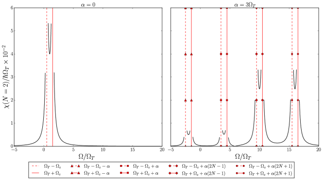
Figure 1: Dispersive shift $\chi(N)$ as function of $\Omega$. Panel 1: Without anharmonicity (i.e. $\alpha=0$), we identify the two poles of Eq. (30) with a dashed and a solid line. Between these we note the presence of a single plateau which denotes the resolution for the absorption peaks of the selected transitions. Panel 2: A strong anharmonicity, $\alpha=3\Omega_{T}$, separates the poles of Eq. (30) giving rise to seven separate plateaus, whose boundaries are represented by the marked lines in the plot. Common parameters: $g=0.05\Omega_{T}$, $N=2$ and $\Omega_{z}=\frac{1}{2}\Omega_{T}$, which puts us well within the dispersive regime conditions for almost all values of $\Omega$. Whenever that was not the case, we omitted to plot those lines.

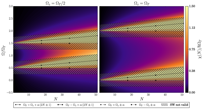
Figure 2: Dispersive shift $\chi(N)$ as function of $N$ and $\Omega$ with a small anharmonicity of $\alpha=0.003\Omega_{T}$ and $g=0.05\Omega_{T}$. The primary goal of these plots is to examine the effect of varying $N$ and the Zeeman splitting. Panel 1: $\Omega_{z}=\Omega_{T}/2$. Panel 2: $\Omega_{z}=\Omega_{T}$. The solid lines indicate the positions of the divergences which depend on $N$, while the two divergences that remain constant across all $N$ values are represented by dashed lines. The key difference between the two panels is that the separation between divergences is determined by $2\Omega_{z}$. Additionally, the plot shows that as $N$ increases, the value of $\chi(N)$ on the plateau between the divergences also rises, with a more pronounced increase occurring as $\Omega_{z}$ decreases.

IV Dispersive shift in anharmonic, time dependent systems

In this section, we apply the methods developed in the earlier sections to analyze a system composed of a two-level system (TLS) with frequency $\Omega_{z}$, coupled to an anharmonic resonator with frequency $\Omega_{T}$, characterized by an anharmonicity $\alpha$. The interaction between these two systems is mediated by a periodic, time-dependent coupling with frequency $\Omega$. The unperturbed Hamiltonian $\mathcal{H}^{(0)}$ and the perturbation $V(t)$ are given by

$$H_{0}=\hbar\Omega_{T}a^{\dagger}a+\hbar\alpha\left(a^{\dagger}a\right)^{2}+\frac{\hbar\Omega_{z}}{2}\sigma_{z},$$ (22)

$$V(t)=g\left(e^{i\Omega t}a+e^{-i\Omega t}a^{\dagger}\right)\sigma_{x}.$$ (23)

Similar systems have been extensively studied in the literature Xu et al. (2024); Rudin and Reinecke (2001); Xiao et al. (2022); Wang et al. (2023b). However, the inclusion of anharmonic effects combined with the lack of a systematic perturbative approach would either require a suitable ansatz for $S$, expensive computations, or otherwise a Hilbert space truncation to tackle the problem analytically Petrescu et al. (2023); Li et al. (2022); Itoko et al. (2024); Malekakhlagh and Magesan (2022). Additionally, the model described by Eqs. (22),(23) incorporates all the necessary components to make full use of the theoretical framework developed in this article, such as an anharmonicity, an interaction between finite and infinite-dimensional systems, as well as the influence of periodic time-dependent driving. Therefore, the primary purpose of analyzing this system is to demonstrate the applicability of the presented methods, rather than to uncover new physics in this class of systems.

Here, we focus on the dispersive shift $\chi(N)$ (for $N\equiv a^{\dagger}a$) of the anharmonic resonator, which arises from its coupling with the TLS in the dispersive regime $g\ll\omega_{\mu\nu}^{\Delta}-\hbar\Omega,\forall{~{}\mu,\nu,\Delta}$. The dispersive shift $\chi(N)$ represents the resolution in the energy gap between the energy of the $\ket{0}$ and $\ket{n}$ states of the resonator, conditioned on the state of the TLS. In similar systems, $\chi(N)$ plays a crucial role in dispersive readout processes, as a larger dispersive shift enables more precise and reliable determination of the system’s state.

To begin our analysis, we rewrite Eq. (22) and Eq. (23) in the form of Eq. (8) and Eq. (10) respectively. We thus identify

$$f_{\mu}(N)=\begin{cases}\hbar\Omega_{T}a^{\dagger}a+\hbar\alpha\left(a^{\dagger}a\right)^{2}+\frac{\hbar\Omega_{z}}{2}&\text{for }\mu=0,\\ \hbar\Omega_{T}a^{\dagger}a+\hbar\alpha\left(a^{\dagger}a\right)^{2}-\frac{\hbar\Omega_{z}}{2}&\text{for }\mu=1.\end{cases}$$ (24)

and because $\Delta\in\{1\}$

$$g^{(1)}_{\mu\nu}(N)=\begin{cases}ge^{i\Omega t}&\text{for }\mu\neq\nu,\\ 0&\text{for }\mu=\nu.\end{cases}.$$ (25)

We then use Eq. (18) to establish $S(t)$, such that $\left[\mathcal{H}^{(0)},S(t)\right]=-V(t)+i\hbar\frac{\partial S(t)}{\partial t}$. With this we then find the effective Hamiltonian to second order

$$\mathcal{H}_{\text{eff}}=\mathcal{H}^{(0)}+\frac{1}{2}\left[V(t),S(t)\right]=\mathcal{H}^{(0)}+\frac{g^{2}}{2}\mathcal{H}^{\text{corr.}}$$ (26)

Here

$$\mathcal{H}^{\text{corr.}}\equiv -\sum_{\mu\neq\nu}\left(\frac{1}{\omega_{\mu\nu}^{(1)}-\hbar\Omega}-\frac{1}{\omega_{\nu\mu}^{(-1)}+\hbar\Omega}\right)\sigma_{\mu\mu}+\left(-\frac{1}{\omega^{(-1)}_{01}+\hbar\Omega}+\frac{1}{\omega^{(1)}_{10}-\hbar\Omega}+\frac{1}{\omega^{(-1)}_{10}+\hbar\Omega}-\frac{1}{\omega^{(1)}_{01}-\hbar\Omega}\right)a^{\dagger}a\sigma_{z}+$$

$$+\left[e^{2i\Omega t}\left(\frac{1}{\omega^{(1)}_{10}-\hbar\Omega}-\frac{1}{\omega^{(1)}_{01}-\hbar\Omega}\right)a^{2}+e^{-2i\Omega t}\left(\frac{1}{\omega^{(-1)}_{10}+\hbar\Omega}-\frac{1}{\omega^{(-1)}_{01}+\hbar\Omega}\right)\left(a^{\dagger}\right)^{2}\right]\sigma_{z},$$ (27)

where

$$\frac{\omega_{\mu\nu}^{(\pm 1)}}{\hbar}=(-1)^{\nu}\Omega_{z}\pm\Omega_{T}\pm\alpha\left(2N\mp 1\right),\quad\mu\neq\nu.$$ (28)

As mentioned, the dispersive shift $\chi(N)$ is interpreted as the resolution in the energy gap between the energy of the $\ket{0}$ and $\ket{n}$ energy state of the resonator given an energy state of the TLS

$$\chi(N)=\left|\left(\varepsilon_{n,0}-\varepsilon_{0,0}\right)-\left(\varepsilon_{n,1}-\varepsilon_{0,1}\right)\right|,$$ (29)

where $\varepsilon_{n,s}$ is the energy of the $\ket{n,s}$ state of the total system. With Eq. (26) we recover the expression for the dispersive shift using Eq. (29)

$$\chi(N)= \frac{g^{2}}{2\hbar}\left|\frac{-2N-1}{\alpha+2\alpha N+\Omega_{T}-\Omega_{z}-\Omega}+\frac{2N+1}{\alpha-2\alpha N-\Omega_{T}+\Omega_{z}+\Omega}+\frac{2N+1}{-\alpha+2\alpha N+\Omega_{T}+\Omega_{z}-\Omega}+\right.$$

$$+\frac{2N+1}{\alpha+2\alpha N+\Omega_{T}+\Omega_{z}-\Omega}+\frac{1}{\alpha-\Omega_{T}-\Omega_{z}+\Omega}+\frac{1}{\alpha+\Omega_{T}-\Omega_{z}-\Omega}+$$

$$\left.-\frac{1}{\alpha-\Omega_{T}+\Omega_{z}+\Omega}+\frac{1}{\Omega-\alpha-\Omega_{T}-\Omega_{z}}\right|.$$ (30)

From Eq. (30) we notice eight distinct divergence values for $\Omega$, four of which are linearly dependent on the number operator $N$. This dependence on $N$ is strictly contingent on the anharmonicity of Eq. (22) and will play a role in controlling the dispersive shift $\chi(N)$. In the limit of zero anharmonicity (i.e. $\alpha=0$), the eight poles contract into two unique divergences for $\Omega$. These can be observed in Panel 1 of Fig. 1 where we show the dispersive shift as a function of the driving frequency $\Omega$ for $\alpha=0$ and $N=2$. Here the two divergences enclose a single non-zero valued plateau for $\chi(N)$ which defines the distance between the absorption peaks of the $\ket{n=2,0}\rightleftharpoons\ket{n=0,0}$ and $\ket{n=2,1}\rightleftharpoons\ket{n=0,1}$ transitions. Furthermore, in Panel 2 of Fig. 1 we plot $\chi(N)$ for $\alpha=3\Omega_{T}$ and $N=2$. The non zero anharmonicity of the system now splits the poles of the dispersive shift as a function of $\Omega$, thus leading to the formation of seven separate plateaus of $\chi(N)$. As previously mentioned, this splitting effect is strictly dependent on the system’s anharmonicity being non-zero.

It is important to note that the effective Hamiltonian has been derived without a truncation of the bosonic subspace, which allows us to know which divergences, and corresponding plateaus, in $\chi(N)$ along the $\Omega$ domain linearly depend on the mode number $N$. From Eq. (30) we also see the effects of the Zeeman splitting of the TLS in determining the broadness of the plateaus of $\chi(N)$. In particular we find four of the plateaus to have a broadness of $2\Omega_{z}$, while the remaining have broadness $2\Omega_{z}+2\alpha$ (as shown in Fig. (1)). Together with modifying the broadness of the plateaus, the Zeeman splitting of the TLS also plays a role in their height. By inspection of Eq. (30), we can extract that the height of all the plateaus is inversely proportional to $\Omega_{z}$, while the height of the plateaus in between N-dependent divergences is proportional to $N$.

In Fig. 2 we show these features by plotting $\chi(N)$ as a function of the driving frequency $\Omega$ and $N$ for two different values of $\Omega_{z}$. We have chosen a small anharmonicity for simplicity, which results in the collapse of the divergences to only four distinct lines, shown with dashed and solid lines. First, in both Panels we see the effect of the linear dependence on $N$ of the plateaus boundaries, which are represented by the poles of Eq. (30). Moreover, we can see the linear increase in $N$ and the decrease in $\Omega_{z}$ of the height of the plateau.

V Summary

In summary this article introduces a novel, systematic approach to the SWT, a perturbation theory extensively used in quantum mechanics to simplify the study of Hamiltonians by decoupling low and high-energy subspaces. This new methodology offers a general solution for constructing effective Hamiltonians without the need for heuristic assumptions or the truncation of Hilbert spaces, making it applicable to both finite, infinite-dimensional systems and their combinations. The framework is also extended to accommodate time-dependent systems, for which we derived a solution for time-periodic perturbations.

To exemplify the utility of the approach, we have applied it here to the case of a TLS coupled via a time-periodic term to an anharmonic resonator. We have extracted the N-dependent dispersive shift, demonstrating the power of the treatment to get analytical insight.

We hope that this integrated method, combining previously established techniques found in the literature, will prove to be a highly versatile and effective tool for the study of otherwise complicated quantum mechanical systems. Additionally, exploiting the modular nature of the presented solutions, we implemented these results in a systematic software library Leander Reascos (2024). This software takes advantage of the presented general solution to be superior both in applicability and easeness of use to existing libraries Day et al. (2024)

VI Acknowledgements

We acknowledge useful discussions with Maximilian Rimbach-Russ. FGD and MB acknowledge funding from the Emmy Noether Programme of the German Research Foundation (DFG) under grant no. BE 7683/1-1.

Appendix A Multiple bosonic subspaces

In this section, we derive a general expression for the $S$ generator for the scenarios in which the system’s total Hilbert space can be decomposed as $\mathds{H}=\bigotimes_{j=0}^{M-1}\mathds{H}_{j}\otimes\mathds{H}_{f}$, where $\mathds{H}_{j}$ are bosonic Hilbert spaces, while $\mathds{H}_{f}$ is a finite Hilbert space of dimensionality $d_{f}$. Following on the steps of Sec. III, we express the unperturbed Hamiltonian $\mathcal{H}^{(0)}$ for these systems as

$$\mathcal{H}^{(0)}=\sum_{\mu=0}^{d_{f}-1}f_{\mu}(\boldsymbol{\mathrm{N}})\sigma_{\mu\mu},$$ (31)

where $\sigma_{\mu\nu}\equiv|\mu\rangle\langle\nu|$ represents the projectors onto the eigenspace with eigenstates $\{|\mu\rangle\}$ of the finite-dimensional subspace of the system. The term $f_{\mu}(\boldsymbol{\mathrm{N}})$ is instead a general function of the number operators $\boldsymbol{\mathrm{N}}=(N_{0},N_{1},...,N_{M})$ of the bosonic subspaces comprising $\mathds{H}$.

On the other hand, we here postulate that any general hermitian (antihermitian) operator $\mathcal{O}$ acting on $\mathds{H}$ can be reformulated as

$$\mathcal{O}=\sum_{\mu\nu=0}^{d_{f}-1}\sum_{\boldsymbol{\mathrm{\Delta}}}g_{\mu\nu}^{(\boldsymbol{\mathrm{\Delta}})}(\boldsymbol{\mathrm{N}})\boldsymbol{\mathrm{a}}^{\boldsymbol{\mathrm{\Delta}}}\sigma_{\mu\nu}\pm\text{h.c.},$$ (32)

where we introduced the shorthand notation

$$\boldsymbol{\mathrm{a}}^{\boldsymbol{\mathrm{\Delta}}}\equiv\bigotimes_{j=0}^{M-1}a_{j}^{\Delta_{j}}$$ (33)

for $\Delta_{j}\geq 0$ being the label for the subspace within the $j$-th bosonic Hilbert space on which the factor $a_{j}^{\Delta_{j}}$ acts.

From the expression $\left[H^{(0)},S^{(j)}\right]=P^{(j)}$, where $P^{(j)}$ is a perturbation of order $j$ represented by an hermitian operator (see Sec. II.1), and using the commutation relation $\boldsymbol{\mathrm{a}}^{\boldsymbol{\mathrm{\Delta}}}f(\boldsymbol{\mathrm{N}})=f(\boldsymbol{\mathrm{N}}+\boldsymbol{\mathrm{\Delta}})\boldsymbol{\mathrm{a}}^{\boldsymbol{\mathrm{\Delta}}}$, we arrive at a general expression for the anti-hermitian generator $S^{(j)}$

$$s_{\mu\nu}^{(\boldsymbol{\mathrm{\Delta}})}(\boldsymbol{\mathrm{N}})=-\frac{1}{\omega_{\mu\nu}^{(\boldsymbol{\mathrm{\Delta}})}}g_{\mu\nu}^{(\boldsymbol{\mathrm{\Delta}})}(\boldsymbol{\mathrm{N}}),$$ (34)

where

$$\omega_{\mu\nu}^{\boldsymbol{\mathrm{\Delta}}}=f_{\nu}(\boldsymbol{\mathrm{N}}+\boldsymbol{\mathrm{\Delta}})-f_{\mu}(\boldsymbol{\mathrm{N}}).$$ (35)

References

- Villarreal et al. (2022) J. Villarreal, J. Juan, P. Jasen, and J. Ardenghi, Journal of Magnetism and Magnetic Materials 562, 169726 (2022).
- Kale et al. (2022) A. Kale, J. H. Huhn, M. Xu, L. H. Kendrick, M. Lebrat, C. Chiu, G. Ji, F. Grusdt, A. Bohrdt, and M. Greiner, Phys. Rev. A 106, 012428 (2022).
- Voleti et al. (2021) S. Voleti, A. Haldar, and A. Paramekanti, Phys. Rev. B 104, 174431 (2021).
- Hu et al. (2023) H. Hu, B. A. Bernevig, and A. M. Tsvelik, Phys. Rev. Lett. 131, 026502 (2023).
- Manning-Coe and Bradlyn (2023) D. Manning-Coe and B. Bradlyn, Phys. Rev. B 108, 165136 (2023).
- Kolley and Kolley (1990) E. Kolley and W. Kolley, physica status solidi (b) 157, 399–409 (1990).
- Hörmann and Schmidt (2023) M. Hörmann and K. P. Schmidt, SciPost Phys. 15, 097 (2023).
- Lovtsov and Yu. Yushankhai (1991) S. V. Lovtsov and V. Yu. Yushankhai, physica status solidi (b) 166, 209–217 (1991).
- Sun et al. (2021) M. Sun, A. V. Parafilo, K. H. Villegas, V. M. Kovalev, and I. G. Savenko, New Journal of Physics 23, 023023 (2021).
- Weisse et al. (2024) A. Weisse, R. Gerstner, and J. Sirker, Operator growth in disordered spin chains: Indications for the absence of many-body localization (2024), arXiv:2401.08031 [cond-mat.dis-nn] .
- Allard and Weick (2023) T. F. Allard and G. Weick, Phys. Rev. B 108, 245417 (2023).
- Jäger et al. (2022) S. B. Jäger, T. Schmit, G. Morigi, M. J. Holland, and R. Betzholz, Phys. Rev. Lett. 129, 063601 (2022).
- Solgun et al. (2019) F. Solgun, D. P. DiVincenzo, and J. M. Gambetta, IEEE Transactions on Microwave Theory and Techniques 67, 928 (2019).
- Pelegrí et al. (2024) G. Pelegrí, S. Flannigan, and A. J. Daley, Phys. Rev. B 109, 235412 (2024).
- Shani et al. (2022) I. Shani, E. G. Dalla Torre, and M. Stern, Phys. Rev. A 105, 022617 (2022).
- Kawakami et al. (2023) E. Kawakami, J. Chen, M. Benito, and D. Konstantinov, Phys. Rev. Appl. 20, 054022 (2023).
- Hetényi et al. (2022) B. Hetényi, S. Bosco, and D. Loss, Phys. Rev. Lett. 129, 116805 (2022).
- Mutter and Burkard (2021) P. M. Mutter and G. Burkard, Phys. Rev. B 104, 195421 (2021).
- Ansari (2019) M. H. Ansari, Phys. Rev. B 100, 024509 (2019).
- Mutter and Burkard (2020) P. M. Mutter and G. Burkard, Phys. Rev. B 102, 205412 (2020).
- Benito et al. (2019) M. Benito, J. R. Petta, and G. Burkard, Phys. Rev. B 100, 081412 (2019).
- Wang et al. (2021) Z. Wang, E. Marcellina, A. R. Hamilton, J. H. Cullen, S. Rogge, J. Salfi, and D. Culcer, npj Quantum Information 7, 10.1038/s41534-021-00386-2 (2021).
- Liu et al. (2022) Y. Liu, J.-X. Xiong, Z. Wang, W.-L. Ma, S. Guan, J.-W. Luo, and S.-S. Li, Phys. Rev. B 105, 075313 (2022).
- Zhang (2023) Z. Zhang, Annals of Physics 457, 169395 (2023).
- Cayao et al. (2020) J. Cayao, M. Benito, and G. Burkard, Phys. Rev. B 101, 195438 (2020).
- Bosco et al. (2021) S. Bosco, B. Hetényi, and D. Loss, PRX Quantum 2, 010348 (2021).
- Bosco and Loss (2022) S. Bosco and D. Loss, Phys. Rev. Appl. 18, 044038 (2022).
- Del Vecchio and Moutanabbir (2023) P. Del Vecchio and O. Moutanabbir, Phys. Rev. B 107, L161406 (2023).
- Haq et al. (2022) R. U. Haq, B. Iqbal, M. Illahi, B. Ahmad, and Nazama, Schrieffer-wolff transformation on ibm quantum computer (2022), arXiv:2208.04746 [quant-ph] .
- Dey and Schliemann (2024a) B. Dey and J. Schliemann, Phys. Rev. B 109, 155419 (2024a).
- Zhang et al. (2022) Z. Zhang, Y. Yang, X. Xu, and Y. Li, Phys. Rev. Res. 4, 043023 (2022).
- Marécat et al. (2023) Q. Marécat, B. Senjean, and M. Saubanère, Phys. Rev. B 107, 155110 (2023).
- Seedhouse et al. (2021) A. E. Seedhouse, I. Hansen, A. Laucht, C. H. Yang, A. S. Dzurak, and A. Saraiva, Phys. Rev. B 104, 235411 (2021).
- Hillmann and Quijandría (2022) T. Hillmann and F. Quijandría, Phys. Rev. Appl. 17, 064018 (2022).
- Kowalski and Bauman (2022) K. Kowalski and N. P. Bauman, Applied Sciences 13, 539 (2022).
- Fang et al. (2023) Y. Fang, P. Philippopoulos, D. Culcer, W. A. Coish, and S. Chesi, Materials for Quantum Technology 3, 012003 (2023).
- Dey and Schliemann (2024b) B. Dey and J. Schliemann, Role of anisotropic confining potential and elliptical driving in dynamics of a ge hole qubit (2024b), arXiv:2409.03471 [cond-mat.mes-hall] .
- Consani and Warburton (2020) G. Consani and P. A. Warburton, New Journal of Physics 22, 053040 (2020).
- Wang et al. (2023a) D.-W. Wang, C. Zhao, J. Yang, Y.-T. Yan, and L. Zhou, Phys. Rev. A 107, 053701 (2023a).
- Kessler (2012) E. M. Kessler, Phys. Rev. A 86, 012126 (2012).
- von Witte et al. (2024) G. von Witte, S. Kozerke, and M. Ernst, Two-electron two-nucleus effective hamiltonian and the spin diffusion barrier (2024), arXiv:2407.10319 [physics.chem-ph] .
- Massarelli et al. (2022) G. Massarelli, I. Khait, and A. Paramekanti, Phys. Rev. B 106, 144434 (2022).
- Starkov et al. (2023) G. A. Starkov, M. V. Fistul, and I. M. Eremin, Phys. Rev. B 108, 235417 (2023).
- Aramthottil et al. (2022) A. S. Aramthottil, U. Bhattacharya, D. González-Cuadra, M. Lewenstein, L. Barbiero, and J. Zakrzewski, Phys. Rev. B 106, L041101 (2022).
- Magesan and Gambetta (2020) E. Magesan and J. M. Gambetta, Phys. Rev. A 101, 052308 (2020).
- Kehrein and Mielke (1996) S. K. Kehrein and A. Mielke, Annals of Physics 252, 1–32 (1996).
- Salomaa (1988) M. M. Salomaa, Phys. Rev. B 37, 9312 (1988).
- Lee et al. (2017) S.-S. B. Lee, J. von Delft, and A. Weichselbaum, Phys. Rev. B 96, 245106 (2017).
- Malekakhlagh et al. (2020) M. Malekakhlagh, E. Magesan, and D. C. McKay, Phys. Rev. A 102, 042605 (2020).
- Tzen Ong and Jones (2011) T. Tzen Ong and B. A. Jones, EPL (Europhysics Letters) 93, 57004 (2011).
- Wurtz et al. (2020) J. Wurtz, P. W. Claeys, and A. Polkovnikov, Phys. Rev. B 101, 014302 (2020).
- Thomas et al. (2009) C. Thomas, A. S. da Rosa Simões, C. Lacroix, J. Iglesias, and B. Coqblin, Physica B: Condensed Matter 404, 3008–3010 (2009).
- Li et al. (2022) B. Li, T. Calarco, and F. Motzoi, PRX Quantum 3, 030313 (2022).
- Schrieffer and Wolff (1966) J. R. Schrieffer and P. A. Wolff, Phys. Rev. 149, 491 (1966).
- Kim et al. (2021) D.-H. Kim, S.-Y. Lee, Y. Jo, D. Y. Kim, Z. Kim, and T. Jeong, Entropy 23, 1260 (2021).
- Winkler (2003) R. Winkler, Spin-orbit coupling effects in two-dimensional electron and hole systems, Springer tracts in modern physics (Springer, Berlin, 2003).
- Ban (2011) M. Ban, Journal of Modern Optics 58, 640 (2011), https://doi.org/10.1080/09500340.2011.563326 .
- Shen et al. (2022) L.-T. Shen, C.-Q. Tang, Z. Shi, H. Wu, Z.-B. Yang, and S.-B. Zheng, Phys. Rev. A 106, 023705 (2022).
- Guo et al. (2022) Y.-T. Guo, F. Zou, J.-F. Huang, and J.-Q. Liao, Phys. Rev. A 105, 013705 (2022).
- Landi (2024) G. T. Landi, Eigenoperator approach to schrieffer-wolff perturbation theory and dispersive interactions (2024), arXiv:2409.10656 [quant-ph] .
- Wysokiński et al. (2021) M. M. Wysokiński, M. Płodzień, and M. Trif, Phys. Rev. B 104, L041402 (2021).
- Sentef et al. (2020) M. A. Sentef, J. Li, F. Künzel, and M. Eckstein, Phys. Rev. Res. 2, 033033 (2020).
- Malekakhlagh et al. (2022) M. Malekakhlagh, E. Magesan, and L. C. G. Govia, Phys. Rev. A 106, 052601 (2022).
- Goldin and Avishai (2000) Y. Goldin and Y. Avishai, Phys. Rev. B 61, 16750 (2000).
- Murakami et al. (2021) Y. Murakami, S. Takayoshi, A. Koga, and P. Werner, Phys. Rev. B 103, 035110 (2021).
- Wang et al. (2024) X. Wang, F. P. M. Méndez-Córdoba, D. Jaksch, and F. Schlawin, Floquet schrieffer-wolff transform based on sylvester equations (2024), arXiv:2407.08405 [quant-ph] .
- Bukov et al. (2016) M. Bukov, M. Kolodrubetz, and A. Polkovnikov, Phys. Rev. Lett. 116, 125301 (2016).
- Romhányi et al. (2015) J. Romhányi, G. Burkard, and A. Pályi, Phys. Rev. B 92, 054422 (2015).
- Petrescu et al. (2023) A. Petrescu, C. Le Calonnec, C. Leroux, A. Di Paolo, P. Mundada, S. Sussman, A. Vrajitoarea, A. A. Houck, and A. Blais, Phys. Rev. Appl. 19, 044003 (2023).
- Xu et al. (2024) Y. Xu, F.-X. Sun, Q. He, H. Pu, and W. Zhang, Phys. Rev. A 110, 023702 (2024).
- Rudin and Reinecke (2001) S. Rudin and T. L. Reinecke, Phys. Rev. B 63, 075308 (2001).
- Xiao et al. (2022) Z. Xiao, E. Doucet, T. Noh, L. Ranzani, R. Simmonds, L. Govia, and A. Kamal, Phys. Rev. Appl. 18, 024009 (2022).
- Wang et al. (2023b) Y. Wang, Z. You, and H. Ian, AVS Quantum Science 5, 036201 (2023b), https://pubs.aip.org/avs/aqs/article-pdf/doi/10.1116/5.0159488/18113922/036201_1_5.0159488.pdf .
- Itoko et al. (2024) T. Itoko, M. Malekakhlagh, N. Kanazawa, and M. Takita, Phys. Rev. Appl. 21, 034018 (2024).
- Malekakhlagh and Magesan (2022) M. Malekakhlagh and E. Magesan, Phys. Rev. A 105, 012602 (2022).
- Leander Reascos (2024) G. F. D. Leander Reascos, Monica Benito, In preparation (2024).
- Day et al. (2024) I. A. Day, S. Miles, H. K. Kerstens, D. Varjas, and A. R. Akhmerov, Pymablock: an algorithm and a package for quasi-degenerate perturbation theory (2024), arXiv:2404.03728 [quant-ph] .