Quantum Fisher information of a cosmic qubit undergoing non-Markovian de Sitter evolution

Abstract

We revisit the problem of thermalization process for an Unruh-DeWitt (UDW) detector in de Sitter space. We derive the full dynamics of the detector in the context of open quantum system, neither using Markovian or RWA approximations. We utilize quantum Fisher information (QFI) for Hubble parameter estimation, as a process function to distinguish the thermalization paths in detector Hilbert space, determined by its local properties, e.g., detector energy gap and its initial state preparation, or global spacetime geometry. We find that the non-Markovian contribution in general reduces the QFI comparing with Markovian approximated solution. Regarding to arbitrary initial states, the late-time QFI would converge to an asymptotic value. In particular, we are interested in the background field in the one parameter family of $\alpha$-vacua in de Sitter space. We show that for general $\alpha$-vacuum choices, the asymptotic values of converged QFI are significantly suppressed, comparing to previous known results for Bunch-Davies vacuum.

1 Introduction

The quantum field theory in de Sitter space is a recurrent concern over several decades. This is partially because of that de Sitter space is an analytically tractable curved solution of Einstein equation with maximal symmetry. Also, it plays a key role in modern cosmology as that the exponentially expanding de Sitter patch predicts the evolution of universe during cosmic inflation and at far future when dark energy dominates. However, the exact behavior of quantum fields in de Sitter space appears to be very exclusive DS1 . For example, even neglecting issues of back-reaction, the QFT in de Sitter becomes catastrophic from the view of local observers, e.g., the usual S-matrix intuition of local quantum field theory seems to fail dS1 .

An important tool for unveiling the properties of quantum fields within specific spacetime geometry is Unruh-DeWitt (UDW) detector UDW1 ; UDW2 , which is a microscopic two-level quantum system (qubit) coupled locally to fluctuating backgrounds. From a detector-field-interaction perspective, the response function for an UDW detector represents the rate of quantum transition occurring per unit proper time, determined by the quantum fields propagators w.r.t. interested spacetime geometry UDW3 . For example, for an accelerated UDW detector in flat spacetime, the periodic correlation functions in Rindler geometry lead to celebrated Unruh radiation locally perceived by the detector UDW4 . Outside a static black hole, with respect to a Hartle-Hawking vacuum UDW5 , the detector would be excited to an equilibrium with Planck-distributed spectrum, referred as Hawking effect UDW6 . Back to de Sitter story, it was shown dS12-1 that a comoving UDW detector will perceive radiation with a thermal spectrum of temperature $T_{H}=H/2\pi$, where $H$ denotes the Hubble parameter. This so-called Gibbons-Hawking effect is quite universal for various kinds of quantum fields. Even for a massless scalar dS12-2 , its infrared divergent propagator only leads to an irrelevant contribution which is insensitive to the total detector response.

Essentially, what detector-field method has given is a local manifestation of so-called thermalization theorem in curved spacetime UDW7 . The method determines the detector equilibrium with background fields which is an unique thermalization end, whose thermal nature can be justified by the detailed-balance condition or the Kubo-Martin-Schwinger (KMS) condition of response function UDW8 . However, this approach cannot capture the full dynamics of the detector, i.e., we cannot know about how the off-diagonal terms (coherence) of detector density matrix evolve during thermalization process. Indeed, arriving at same equilibrium characterized by specific temperature does not means UDW9 that the detector should evolve along the same thermalization path in Hilbert space.

To fully explore the dynamical nature of quantum fields in general curved spacetimes, in recent years, an alternative perspective of open quantum system was intensively used, especially for determining the complete dynamics of UDW detectors in various backgrounds Open1-1 ; Open1-2 ; Open1-3 ; Open1-4 ; Open1-5 . In this context, UDW detector is viewed as a local open system, while background quantum fluctuations play the role of environment inducing dissipation and decoherence. The method is particularly powerful for tracking the long-time process of UDW detector, such as its thermalization undergone Hawking-Unruh or Gibbons-Hawking effects.

Once knowing the dynamics of a detector, the pressing problem is naturally to find some process functions to characterize time-evolution details of open process. Beyond response functions, many important feature functions have been proposed, such as the time-dependent entropic uncertainty bound Open2 ; Open3 , geometric phase of the detector Open4 ; Open5 , as well as the quantum coherence, a critical resource for the non-equilibrium entropy production of the UDW detector during thermalization Open6 .

In this paper, we revisit the dynamics of an UDW detector in de Sitter space within open quantum system context. Accompanying many previous studies Open1-3 ; dS12 ; dS13 ; dS14 , we take further steps based on following considerations:

Firstly, to obtain a resolvable semigroup master equations of the UDW detector, several assumptions are always made Open1 , i.e., (1) Born approximation assuming a weak coupling between system and environment, (2) Markov approximation for memoryless evolution of system leading a time-local master equation, and (3) rotating wave approximation (RWA) neglecting all rapidly oscillating terms near system resonance. However, it has been argued in many ways that these assumptions may only be allowed within a quite restricted parameter space dS15-1 , and even worse the key Markov approximation turns out to be very drastic for early-time dynamics of an UDW detector dS15-2 ; dS15-3 . Thus, to fully explore the dynamics of UDW detector at both early-time and late-time, the non-Markovian contribution of its open process must be taken into account.

Secondly, the QFT in de Sitter itself is complicated by the existence of infinite vacua consistent with CPT invariance, labeled by a superselection parameter $\alpha$ dS2 ; dS3 . Of this vacua family, the well-known Bunch-Davies vacuum (with $\alpha\rightarrow-\infty$) uniquely extrapolates to the Minkowski vacuum in the limit of vanishing cosmological constant, while other vacua can formally be realized as squeezed states over the Bunch-Davies one. Understanding whether interacting field theory in any $\alpha$-vacua is a consistent theory dS4 ; dS5 ; dS6 ; dS7 and how can this provide a better understanding of new physics at Planck-scale of early universe dS8 ; dS9 ; dS8+ or even in holographic scenarios dS10 ; dS11 are still a matter of debate. Thus, accompanying previous studies of UDW detector model in Bunch-Davies vacuum, we would like to extend the analysis to a model within general $\alpha$-vacua.

In this study, we investigate a comoving UDW detector in the $(3+1)$-dimensional de Sitter spacetime, modeled by a two-level system that interacts weakly with massless scalar fields. The structure of the paper is as follows:

In Section 2.1, we induce the master equation of detector. While most previous analysis relying on Markov approximation to simplify the calculation, we appeal neither Markov or RWA approximations. The solution of the equation and its dynamical features for de Sitter backgrounds are analyzed in Section 2.3, with a consideration of delicate choice of $\alpha-$vacua for the background correlation functions given in Section 2.2. Our work extends earlier studies dS15-2 ; dS15-3 of non-Markovian evolution of an uniformly accelerating qubit in flat spacetime, but differs in that the detailed calculations of the residues of the inverse Laplace-transformed density matrix elements in de Sitter space. This improvement is required to avoid the solutions diverge logarithmically and match the initial conditions as $\tau\rightarrow 0^{+}$.

Once obtaining the non-Markovian dynamics of the detector with respect to de Sitter $\alpha-$vacua, in Section 3, we use quantum Fisher information (QFI) as a process function to distinguish thermalization paths of the comoving UDW detector, undergoing the Gibbons-Hawking radiation from the cosmological horizon. This is because as an operational measure on the distinguishability of quantum states, QFI can discriminate parameterized states $\rho(X)$ and $\rho(X+\delta X)$ with infinitesimal change of parameter $X$ (summarized in Section 3.1). Intensive works have been made on utilizing QFI to probe extremely sensitive quantum gravity effects Open8-1 ; Open8-2 ; Open8-3 or spacetime structure Open8-4 ; Open8-6 ; Open8-7 .

In Section 3.2, we argue that with $H$ as a parameter chosen to be metrologically estimated, given the explicit dynamics of comoving UDW detector, the related time-evolving QFI $\mathcal{F}_{Q}(H)$ can distinguish the non-Markovian dynamics from those inherited from Markov approximation. We find that after a sufficient long time, the $\mathcal{F}_{Q}(H)$ approaches an asymptotic value Open8-5 , which is irrelevant with detector initial state preparation. However, with varying Hubble parameter or de Sitter vacuum-choices, the asymptotic value of QFI and the ways detector approaching it would be modified.

Throughout the paper, we use units with $G=c=\hbar=k_{B}=1$.

2 The non-Markovian evolution in de Sitter space

2.1 Model setting

The UDW detector is modeled by an idealized point particle with two internal energy levels, described by a $2\times 2$ Hamiltonian

$$H_{S}=\frac{\omega}{2}(\vec{n}\cdot\vec{\sigma}),$$ (1)

where $\sigma_{i}$ are the Pauli matrices, $\vec{n}$ is a unit vector, and $\omega$ is the energy gap of the two level system.

For the detector moving along a particular trajectory $x(\tau)$ in the given spacetime $\mathcal{M}$, we consider it weakly interacts with some massless scalar fields $\phi_{\alpha}(x)$ through the Hamiltonian

$$H_{I}(\tau)=g\sum_{i=1}^{3}\sigma^{i}(\tau)\otimes\Phi_{i}(\tau),$$ (2)

where $\Phi_{i}(\tau)=\sum_{\alpha}\chi_{i}^{\alpha}\phi_{\alpha}(x(\tau))$ are linear combinations of field operators, $g$ is a small coupling and $\sigma^{i}(\tau)$ is generated by a time translations $\mathcal{U}_{\tau}$ as $\sigma^{i}(\tau)\equiv\mathcal{U}_{\tau}[\sigma^{i}]=e^{iH_{S}\tau}\sigma^{i}e^{-iH_{S}\tau}$.

In the interaction picture, the evolution of the density matrix $\rho_{\text{tot}}$ of combined system is governed by

$$\dot{\rho}_{\text{tot}}(\tau)=-i[H_{I}(\tau),\rho_{\text{tot}}(\tau)].$$ (3)

In the weak coupling regime, the Born’s approximation can be employed

$$\rho_{\text{tot}}(\tau)\approx\rho(\tau)\otimes\rho_{\Phi},$$ (4)

where $\rho(\tau)=\mathrm{Tr}_{\mathrm{B}}\left[\rho_{\text{tot}}\right]$ is the reduced density matrix of the detector, while $\rho_{\Phi}$ is the state of background fields. In order to simplify the treatment and write down the explicit expressions for the time-evolved state of an UDW detector, we further assume that $[H_{\Phi},\rho_{\Phi}]=0$ as well as $\langle\phi_{\alpha}(x)\rangle=0$, thus the correlation functions of $\phi_{\alpha}$ takes the form

$$\left\langle\phi_{\alpha}(x(\tau))\phi_{\beta}(x(s))\right\rangle=\delta_{\alpha\beta}\Delta^{+}(\tau-s),$$ (5)

where $\Delta^{+}(\tau-s)=\langle 0|{\phi}[x(\tau)]{\phi}[x(s)]|0\rangle$ is standard Wightman function for a single field, and $\Delta^{-}(\tau)\equiv\Delta^{+}(\tau)^{*}$ is also defined for later use.

Under these assumptions, the evolution of the detector density matrix $\rho(\tau)$ is reduced to an integro-differential master equation Open1 ; dS15-2

$$\dot{\rho}(\tau)=g^{2}\sum_{i=1}^{3}\int_{0}^{\tau}ds\,[\sigma^{i}(s)\rho(s),\sigma^{i}(\tau)]\Delta^{+}(\tau-s)+h.c.$$ (6)

One may note that during the derivation of (6), neither Markov approximation or RWA approximation have been employed. The evolution equation (6) is indeed non-Markovian, in the sense that $\dot{\rho}(\tau)$ depends on the history $\rho(s)$ for all $s\leq\tau$, instead of depending on $\rho(\tau)$ alone. Moreover, it is worth to be emphasized that the non-Markovian master equation (6) is accurate to $O(g^{4})$ order Master1 , guaranteed in the limitation of Born’s approximation.

Before proceeding, we employ an alternative basis to simplify the master equation. Introducing three complex vectors $\vec{\xi}^{(\mu)}$ with $\mu=0,\pm 1$, so that

$$\vec{\xi}^{(0)}\equiv\vec{n},\quad\vec{\xi}^{(\mu)}\cdot\vec{\xi}_{(\nu)}^{*}=\delta^{\mu}_{\nu},\quad\vec{\xi}^{(\mu)}\times\vec{\xi}^{(\nu)}=i\sum_{\gamma=0,\pm}\epsilon^{\mu\nu\gamma}\;\vec{\xi}_{(\gamma)}^{*},$$ (7)

where $\vec{\xi}_{(\mu)}^{*}=\vec{\xi}^{(-\mu)}$, and $\epsilon^{\alpha\beta\gamma}$ is completely anti-symmetric with $\epsilon^{1,0,-1}=1$. It is straightforward to verify that these vectors form a complete basis

$$\sum_{\mu=0,\pm}(\vec{\xi}^{*}_{(\mu)})^{i}(\vec{\xi}^{(\mu)})_{j}=\delta^{ij},$$ (8)

by which the original Pauli matrices $\sigma^{i}$ can be projected to $\sigma^{(\mu)}\equiv\vec{\xi}^{(\mu)}\cdot\vec{\sigma}$, evolving under time translation operator as

$$\sigma^{(\mu)}(\tau)=\mathcal{U}_{\tau}[\sigma^{(\mu)}]=e^{iH_{S}\tau}\left(\vec{\xi}^{(\mu)}\cdot\vec{\sigma}\right)e^{-iH_{S}\tau}=e^{i\mu\omega\tau}\sigma^{(\mu)}.$$ (9)

In terms of $\sigma^{(\mu)}$, the non-Markovian master equation (6) can now be recasted into

$$\dot{\rho}(\tau)=g^{2}\sum_{\mu=0,\pm}\int_{0}^{\tau}ds\,[\sigma^{{\dagger}}_{(\mu)}\rho(s),\sigma^{(\mu)}]\Delta^{+}(\tau-s)e^{i\mu\omega(\tau-s)}+h.c.$$ (10)

For a single detector (qubit), its density matrix can be decomposed in a Bloch-like form

$$\rho(\tau)=\frac{1}{2}\left(1+\sum_{\mu=0,\pm}v_{(\mu)}(\tau)\sigma^{(\mu)}\right).$$ (11)

Benefited from the fact that $\sigma^{(\mu)}$ are eigenvectors of $\mathcal{U}_{\tau}$ which also commutes with (6), the time evolution of coefficients $v_{(\mu)}(\tau)$ in new basis now decouples Open1-1 . For instance, without loss of generality, we can choose $\vec{n}=\hat{z}$ in (1), which gives $\vec{\xi}^{(0)}=\hat{z}$ and $\vec{\xi}^{(\pm)}=\frac{1}{\sqrt{2}}(\hat{x}\pm i\hat{y})$. Then the decomposition (11) is explicitly given as

$$\rho=\frac{1}{2}\begin{bmatrix}1+v_{(0)}&&\sqrt{2}v_{(+)}\\ \sqrt{2}v_{(-)}&&1-v_{(0)}\end{bmatrix},$$ (12)

where $v_{(0)}=\rho_{11}-\rho_{00}$ determines the time-evolution of diagonal elements, and $v_{(\pm)}$ determines the time-evolution of off-diagonal elements of detector qubit.

We are now in a position to explicitly solve the non-Markovian master equation (10). Noting that (10) admits a form of a convolution, we employ a Laplace transformation and obtain

$$z\tilde{\rho}(z)-\rho(0)=g^{2}\sum_{\mu=0,\pm}[\sigma^{{\dagger}}_{(\mu)}\tilde{\rho}(z),\sigma^{(\mu)}]\tilde{\Delta}^{+}(z-i\mu\omega)+h.c.$$ (13)

where $\tilde{\Delta}^{+}$ is the Laplace-transformed Wightman function, and the Laplace-transformed density matrix $\tilde{\rho}(z)$ from (12) admits a similar Bloch-decomposition

$$\tilde{\rho}(z)=\frac{1}{2}\left(\frac{1}{z}+\sum_{\mu=0,\pm}\tilde{v}_{(\mu)}(z)\sigma^{(\mu)}\right).$$ (14)

The time-evolution of the coefficients $\tilde{v}_{(\mu)}$ can be given explicitly (for details see Appendix A)

$$\left\{\begin{aligned} \tilde{v}_{(0)}(z)&=\frac{\left.v_{(0)}\right|_{\tau=0}+2g^{2}M(z)/z}{z+2g^{2}N_{(0)}(z)},\\ \tilde{v}_{(\pm)}(z)&=\frac{\left.v_{(\pm)}\right|_{\tau=0}}{z+2g^{2}N_{(\pm)}(z)},\end{aligned}\right.$$ (15)

where the functions $M(z)$, $N_{(\mu)}(z)$ are defined by

$$M(z)\equiv \tilde{\Delta}^{+}(z+i\omega)-\tilde{\Delta}^{-}(z+i\omega)+\tilde{\Delta}^{-}(z-i\omega)-\tilde{\Delta}^{+}(z-i\omega),$$ (16)

$$N_{(0)}(z)\equiv \tilde{\Delta}^{+}(z+i\omega)+\tilde{\Delta}^{-}(z+i\omega)+\tilde{\Delta}^{+}(z-i\omega)+\tilde{\Delta}^{-}(z-i\omega),$$

$$N_{(\pm)}(z)\equiv \tilde{\Delta}^{+}(z\mp i\omega)+\tilde{\Delta}^{-}(z\mp i\omega)+\tilde{\Delta}^{+}(z)+\tilde{\Delta}^{-}(z).$$

Except been written in a more efficient basis, we can check that the results (15) are consistent with those were given in dS15-2 .

Taking inverse Laplace transformation on $\tilde{v}_{(\mu)}(z)$, we recover the coefficients $v_{(\mu)}$ as

$$v_{(\mu)}(\tau)=\frac{1}{2\pi i}\int_{c-i\infty}^{c+i\infty}\mathrm{d}p\,\tilde{v}_{(\mu)}(z)e^{z\tau},$$ (17)

where $c$ is a real constant larger than the real part of all the singularities of integrand Toolbox . Obviously, the time-evolving coefficients $v_{(\mu)}(\tau)$ should depend on the specific correlation functions $\Delta^{\pm}(\tau)$.

2.2 Correlation functions of scalar fields within $\alpha$-vacua

We consider the comoving UDW detector (qubit) interacting with a massless scalar field in expanding de Sitter space. The time evolution is investigated along the direction of planar coordinates, in terms of which the spacetime line-element is

$${d}s^{2}=-\mathrm{d}\tau^{2}+e^{2H\tau}\mathrm{~{}d}\mathbf{x}^{2}=\frac{1}{H^{2}\eta^{2}}\left(-\mathrm{d}\eta^{2}+\mathrm{d}\mathbf{x}^{2}\right),$$ (18)

where $H>0$ is the Hubble parameter, and the conformal time $\eta$ related to comoving time $\tau$ by $\eta=-e^{-H\tau}/H$, which represents a flat slicing of spacetime.

As explained in the introduction, we aim to resolve the time-evolution of UDW detector respecting general de Sitter-invariant vacua of a real scalar field. Within these so-called $\alpha$-vacua, the scalar Wightman function $\Delta^{+}(x,y;\alpha)=\langle\alpha|{\phi}(x){\phi}(y)|\alpha\rangle$ are related to the ones in Bunch-Davies vacuum $\Delta^{+}(x,y)=\langle\text{BD}|{\phi}(x){\phi}(y)|\text{BD}\rangle$ like dS8 ; dS10 ; dS12 :

$$\Delta^{+}(x,y;\alpha)=\frac{1}{1-e^{2\alpha}}\left[\Delta^{+}(x,y)+e^{2\alpha}\Delta^{+}(y,x)+e^{\alpha}(\Delta^{+}(x,y_{A})+\Delta^{+}(x_{A},y))\right],$$ (19)

where $x_{A}$ is the antipodal point of $x$, and the parameter $\alpha$ in $\Delta^{+}(x,y;\alpha)$ labels Wightman functions with respect to different $\alpha-$vacua choice. As $\alpha\rightarrow{-\infty}$, the vacua $|\alpha\rangle$ approaches to Bunch-Davies one $|\text{BD}\rangle$, thus leading $\Delta^{+}(x,y;\alpha)$ reduce to $\Delta^{+}(x,y)$.

For a comoving detector parameterized by its own proper-time, we have Wightman functions in Bunch-Davies vacuum UDW3

$$\left\{\begin{aligned} \Delta^{+}(x(\tau),x(s))=-\frac{H^{2}}{16\pi^{2}\sinh^{2}\left(\frac{H(\tau-s)-i\epsilon}{2}\right)},\\ \Delta^{+}(x_{A}(\tau),x(s))=\frac{H^{2}}{16\pi^{2}\cosh^{2}\left(\frac{H(\tau-s)-i\epsilon}{2}\right)},\\ \Delta^{+}(x(\tau),x_{A}(s))=\frac{H^{2}}{16\pi^{2}\cosh^{2}\left(\frac{H(\tau-s)+i\epsilon}{2}\right)},\end{aligned}\right.$$ (20)

where the parameter $\epsilon$ regularize the divergence at $\tau\rightarrow 0$ with a cutoff scale $\epsilon^{\prime}=\epsilon H$.

Applying a Laplace transformation on $\Delta^{+}(x(\tau),x(0);\alpha)$, we obtain

$$\tilde{\Delta}^{\pm}(z;\alpha)=\frac{1}{1-e^{2\alpha}}\left[E_{(\pm)}(z)+e^{2\alpha}E_{(\mp)}(z)+2e^{\alpha}F(z)\right],$$ (21)

where

$$F(z)\equiv \int_{0}^{\infty}\mathrm{d}\tau\,\left(\frac{\Delta^{+}(x_{A}(\tau),x(0))+\Delta^{+}(x(\tau),x_{A}(0))}{2}\right)e^{-z\tau},$$ (22)

$$E_{(\pm)}(z)\equiv \int_{0}^{\infty}\mathrm{d}\tau\,\Delta^{+}(x(\pm\tau),x(0))e^{-z\tau},$$

which can be explicitly integrated out as (for details see Appendix B)

$$E_{(\pm)}(z)=\frac{H}{8\pi^{2}}\left(\pm\coth{\frac{i\epsilon}{2}}+2z\sum_{n=0}^{\infty}\frac{e^{\pm in\epsilon}}{z+nH}-1\right),$$ (23)

$$F(z)=\frac{H}{8\pi^{2}}\left(2z\sum_{n=0}^{\infty}\frac{(-1)^{n}\cos{n\epsilon}}{z+nH}-1\right).$$

Substituting these back into (21), we obtain the Laplace-transformed correlation functions $\tilde{\Delta}^{\pm}(z;\alpha)$ as

$$\tilde{\Delta}^{\pm}(z;\alpha)=\frac{H}{8\pi^{2}}\left(-\sum_{n=0}^{\infty}\frac{[\coth{\alpha}+(-1)^{n}\operatorname{csch}{\alpha}]\cos{n\epsilon}\mp i\sin{n\epsilon}}{(1+nH/z)/2}-\frac{(1+e^{\alpha})^{2}}{1-e^{2\alpha}}\pm\coth{\frac{i\epsilon}{2}}\right).$$ (24)

We observe that the functions have infinite simple poles at $z_{n}=-nH$ for $n\in\mathbb{Z}^{+}$, with residues like

$$\mathfrak{Res}\left[\tilde{\Delta}^{\pm}(z;\alpha),z_{n}\right]=\frac{H^{2}}{4\pi}\left(n\left[\coth{\alpha}+(-1)^{n}\operatorname{csch}{\alpha}\right]\cos{n\epsilon}\mp in\sin{n\epsilon}\right).$$ (25)

With the help from (25), we can determine the pole structures of the functions $M(z;\alpha)$ and $N_{(\mu)}(z;\alpha)$ respecting different $\alpha-$vacua. For instance, we start with $N_{(0)}(z;\alpha)$ defined by (16) as

$$\begin{aligned} N_{(0)}(z;\alpha)\equiv\tilde{\Delta}^{+}(z+i\omega;\alpha)+\tilde{\Delta}^{-}(z+i\omega;\alpha)+\tilde{\Delta}^{-}(z-i\omega;\alpha)+\tilde{\Delta}^{+}(z-i\omega;\alpha)\end{aligned}.$$ (26)

They have infinite simple poles located at $z_{n}^{\pm}=-Hn\pm i\omega$ for $n\in\mathbb{Z}^{+}$, with corresponding residues

$$\begin{aligned} \mathfrak{Res}\left[N_{(0)}(z;\alpha),z_{n}^{\pm}\right]=\frac{H^{2}n[\coth{\alpha}+(-1)^{n}\operatorname{csch}{\alpha}]\cos{n\epsilon}}{2\pi^{2}}\end{aligned}.$$ (27)

By looking at the functions

$$M(z;\alpha)=\tilde{\Delta}^{+}(z+i\omega;\alpha)-\tilde{\Delta}^{-}(z+i\omega;\alpha)+\tilde{\Delta}^{-}(z-i\omega;\alpha)-\tilde{\Delta}^{+}(z-i\omega;\alpha),$$ (28)

one can tell that they have poles located at $z_{n}^{\pm}$, whose residues can be given as

$$\mathfrak{Res}\left[M(z;\alpha),z_{n}^{\pm}\right]=\pm\frac{iH^{2}n\sin{n\epsilon}}{2\pi^{2}}.$$ (29)

The functions $N_{(\pm)}(z;\alpha)$ have poles at both $z_{n}$ and $z_{n}^{\pm}$, with residues:

$$\mathfrak{Res}\left[N_{(\pm)}(z;\alpha),z_{n}\right]=\mathfrak{Res}\left[N_{(\pm)}(z;\alpha),z_{n}^{\pm}\right]=\frac{H^{2}n[\coth{\alpha}+(-1)^{n}\operatorname{csch}{\alpha}]\cos{n\epsilon}}{2\pi^{2}}.$$ (30)

Collecting above results, we eventually obtain

$$\left\{\begin{aligned} M(z;\alpha)&=\sum_{n=1}^{\infty}\mathfrak{M}_{n}\left(\frac{1}{z+nH-i\omega}-\frac{1}{z+nH+i\omega}\right)+\text{regular},\\ N_{(0)}(z;\alpha)&=\sum_{n=1}^{\infty}\mathfrak{N}_{n}\left(\frac{1}{z+nH-i\omega}+\frac{1}{z+nH+i\omega}\right)+\text{regular},\\ N_{(\pm)}(z;\alpha)&=\sum_{n=1}^{\infty}\mathfrak{N}_{n}\left(\frac{1}{z+nH}+\frac{1}{z+nH\mp i\omega}\right)+\text{regular},\end{aligned}\right.$$ (31)

where the ’regular’ parts are holomorphic in $\mathbb{C}$, and two coefficient functions

$$\mathfrak{M}_{n}=\frac{iH^{2}n\sin{n\epsilon}}{2\pi^{2}},~{}~{}~{}~{}~{}~{}~{}\mathfrak{N}_{n}=\frac{H^{2}n\cos{n\epsilon}\left[(-1)^{n}\operatorname{csch}{\alpha}+\cosh{\alpha}\right]}{2\pi^{2}\sinh{\alpha}}$$ (32)

are introduced to simplify the expression.

2.3 Dynamics of an UDW detector in de Sitter Space

To resolve the non-Markovian dynamics of the comoving UDW detector, we need substitute (31) into (15), then evaluate the inverse Laplace transformation (17), where the coefficient functions $v_{(\mu)}(\tau;\alpha)$ give the time-evolution of detector density matrix through (11). Determined by the pole structure of $M(z;\alpha)$ and $N_{(\mu)}(z;\alpha)$ (with $\mu=0,\pm$), we could recognize the singularities of $\tilde{v}_{(\mu)}(z;\alpha)$ are discrete, therefore express (17) as a sum of residues

$$v_{(\mu)}(\tau;\alpha)=\frac{1}{2\pi i}\int_{c-i\infty}^{c+i\infty}\mathrm{d}z\,\tilde{v}_{(\mu)}(z;\alpha)e^{z\tau}=\sum_{k}\mathfrak{Res}\left[\tilde{v}_{(\mu)}(z;\alpha)e^{z\tau},z_{(\mu),k}\right],$$ (33)

where $\{z_{(\mu),k}\}_{k=1}^{\infty}$ denote the poles of functions $\tilde{v}_{(\mu)}(z;\alpha)$. As shown in (15) that the evolution of coefficients $v_{(\mu)}$ decouples, we treat the diagonal part $v_{(0)}$ and the off-diagonal part $v_{(\pm)}$ (e.g., of the detector density matrix (12)) separately.

2.3.1 The diagonal part

We first determine the pole structure of $\tilde{v}_{(0)}(z;\alpha)$, which is now given as

$$\tilde{v}_{(0)}(z;\alpha)=\frac{\left.v_{(0)}\right|_{\tau=0}+2g^{2}M(z;\alpha)/z}{z+2g^{2}N_{(0)}(z;\alpha)}.$$ (34)

Markovian poles—Since $M(z;\alpha)$ and $N_{(0)}(z;\alpha)$ are analytic at $z=0$, we can find two poles of the function $\tilde{v}_{(0)}(z;\alpha)$ located at $z_{(0),1}=0$ and $z_{(0),2}$, where the later one is determined by the equation

$$z_{(0),2}+2g^{2}N_{(0)}\left(z_{(0),2};\alpha\right)=0$$ (35)

around the point $z=0$. We call $z_{(0),1}=0$ and $z_{(0),2}$ Markovian poles as depicted in Fig.1.

The residue at $z_{(0),1}=0$ is easy to determine as

$$\mathfrak{Res}\left[\tilde{v}_{(0)}(z;\alpha),z_{(0),1}\right]=\frac{M(0;\alpha)}{N_{(0)}(0;\alpha)}.$$ (36)

The residue at $z_{(0),2}$ is more subtle. Based on complex analysis, the result is

$$\mathfrak{Res}\left[\tilde{v}_{(0)}(z;\alpha),z_{(0),2}\right]=\frac{v_{(0)}|_{\tau=0}+2g^{2}M\left(z_{(0),2};\alpha\right)/z_{(0),2}}{1+2g^{2}N^{\prime}_{(0)}\left(z_{(0),2};\alpha\right)}.$$ (37)

where “$\,{}^{\prime}\,$” indicates a derivative with respect to complex variable $z$. Since the the numerator contains contributions of the form $g^{2}/z_{(0),2}$, we have to expand $z_{(0),2}$ to $\mathcal{O}(g^{6})$ to guarantee that the result is accurate to $\mathcal{O}(g^{4})$. From (35), we have the expansion

$$z_{(0),2}\approx-2g^{2}N_{(0)}(0;\alpha)\left(1-2g^{2}N^{\prime}_{(0)}(0;\alpha)\right)+\mathcal{O}(g^{6}).$$ (38)

Combining with (37), we obtain

$$\mathfrak{Res}\left[\tilde{v}_{(0)}(z;\alpha),z_{(0),2}\right]=[1-2g^{2}N^{\prime}_{(0)}(0;\alpha)]v_{(0)}(0;\alpha)+2g^{2}M^{\prime}(0;\alpha)-\frac{M(0;\alpha)}{N_{(0)}(0;\alpha)}+\mathcal{O}(g^{4}),$$ (39)

where $v_{(0)}(0;\alpha)=v_{(0)}|_{\tau=0}$ is the initial value of the coefficient. It is worth noting that our evaluation (39) differs from those in dS15-2 where second and third terms are missing for an accelerating UDW qubit. However, these additional terms are necessary for matching the detector state $\rho(\tau)$ with the initial condition as $\tau\rightarrow 0^{+}$ in de Sitter scenario.

Non-Markovian poles—Since $g$ is small, the only remaining place for $\tilde{v}_{(0)}(z;\alpha)$ to be singular is the neighborhood of $z_{n}^{\pm}=-nH\pm i\omega$, where $M(z;\alpha)$ and $N_{(0)}(z;\alpha)$ are divergent. Therefore, we anticipate that additional sets of (infinite) poles $z_{(0),n}^{\pm}$ near $z_{n}^{\pm}$ should exist, which we call non-Markovian poles based on the insights dS15-2 that their contributions can be ignored for the Markov-approximated master equation of an accelerating UDW qubit.

From (31), we know that in a neighborhood of $z_{n}^{\pm}$,

$$M(z;\alpha)=\pm\frac{\mathfrak{M}_{n}}{z-z_{n}^{\pm}}+f_{M}(z),~{}~{}~{}~{}N_{(0)}(z;\alpha)=\frac{\mathfrak{N}_{n}}{z-z_{n}^{\pm}}+f_{N_{(0)}}(z),$$ (40)

where $f_{M}(z)$ and $f_{N_{(0)}}(z)$ are analytic near $z^{\pm}_{n}$, whose details need not be worried about as they only generate $\mathcal{O}(g^{4})$ contributions in the final results.

The non-Markovian poles $z_{(0),n}^{\pm}$ are determined from

$$z_{(0),n}^{\pm}+2g^{2}N_{(0)}\left(z_{(0),n}^{\pm};\alpha\right)=0,$$ (41)

which can be resolved by the decomposition (40), leading to

$$z_{(0),n}^{\pm}-z_{n}^{\pm}=-\frac{2g^{2}~{}\mathfrak{N}_{n}}{z_{n}^{\pm}+2g^{2}~{}f_{N_{0}}(z_{n}^{\pm})}.$$ (42)

Ignoring higher order contributions in $g$, we obtain (depicted by red points in Fig.1)

$$z_{(0),n}^{\pm}=-nH\pm i\omega+\frac{2g^{2}\mathfrak{N}_{n}}{nH\mp i\omega}+\mathcal{O}(g^{4}).$$ (43)

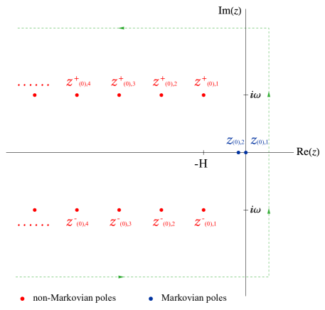
Figure 1: The pole structure of the Laplace-transformed diagonal coefficient $\tilde{v}_{(0)}(z;\alpha)$, where two blue points represent Markovian poles $z_{(0),1}$ and $z_{(0),2}$, and two infinite sets of red points label the non-Markovian poles $z_{(0),n}^{+}$ and $z_{(0),n}^{-}$ ($n\in\mathbb{Z}^{+}$).

Once the non-Markovian poles $z_{(0),n}^{\pm}$ are specified, the residues of coefficient functions $\tilde{v}_{(0)}(z;\alpha)$ at these poles can be calculated from

$$\mathfrak{Res}\left[\tilde{v}_{(0)}(z;\alpha),z_{(0),n}^{\pm}\right]=\frac{\left.v_{(0)}\right|_{\tau=0}+2g^{2}M\left(z_{(0),n}^{\pm};\alpha\right)/z_{(0),n}^{\pm}}{1+2g^{2}N^{\prime}_{(0)}\left(z_{(0),n}^{\pm};\alpha\right)}.$$ (44)

Substituting the straightforwardly calculated results

$$2g^{2}N_{(0)}^{\prime}\left(z_{(0),n}^{\pm};\alpha\right) =-\frac{(nH\mp i\omega)^{2}}{2g^{2}\mathfrak{N}_{n}}+\mathcal{O}(g^{2}),$$ (45)

$$2g^{2}M\left(z_{(0),n}^{\pm};\alpha\right)/z_{(0),n}^{\pm} =\mp\frac{\mathfrak{M}_{n}}{\mathfrak{N}_{n}}+\mathcal{O}(g^{2})$$

into (44), we eventually obtain the desired residue of $\tilde{v}_{(0)}(z;\alpha)$ at non-Markovian poles as

$$\mathfrak{Res}\left[\tilde{v}_{(0)}(z;\alpha),z_{(0),n}^{\pm}\right]=\frac{2g^{2}\left[\pm\mathfrak{M}_{n}-\mathfrak{N}_{n}v_{(0)}(0;\alpha)\right]}{(nH\mp i\omega)^{2}}+\mathcal{O}(g^{4}).$$ (46)

In summary, we find functions $\tilde{v}_{(0)}(z;\alpha)$ have two Markovian poles located at $z_{(0),1}$ and $z_{(0),2}$, and two infinite sequences of non-Markovian poles located at $z_{(0),n}^{+}$ and $z_{(0),n}^{-}$ for $n>0$, respectively. Figure 1 shows the distribution of these poles on the complex plane.

After determining the complete pole structure of the Laplace-transformed diagonal coefficient $\tilde{v}_{(0)}(z;\alpha)$, as well as the corresponding residues, we are in a position to evaluate the inverse Laplace transformation (33), which explicitly gives the diagonal part of an comoving UDW detector state (12) as

$$v_{(0)}(\tau;\alpha)=\gamma_{(0)}\left(e^{-\Gamma_{(0)}\tau}-1\right)+v_{(0)}(0;\alpha)e^{-\Gamma_{(0)}\tau}$$ (47)

$$+2g^{2}\left\{\left[M^{\prime}(0;\alpha)-N^{\prime}_{(0)}(0;\alpha)v_{(0)}(0;\alpha)\right]e^{-\Gamma_{(0)}\tau}+\mathfrak{Re}\left[\sum_{n=1}^{\infty}\frac{2\left[\mathfrak{M}_{n}-\mathfrak{N}_{n}v_{(0)}(0;\alpha)\right]e^{(i\omega-nH)\tau}}{(nH-i\omega)^{2}}\right]\right\},$$

where $\mathcal{O}(g^{4})$ contributions have been ignored, $\mathfrak{Re}$ takes the real part of variable, and two important functions $\gamma_{(0)}$ and $\Gamma_{(0)}$ are defined by (for details see Appendix C)

$$\left\{\begin{aligned} \gamma_{(0)}&\equiv-\frac{M(0;\alpha)}{N_{(0)}(0;\alpha)}=-\frac{\sinh{\alpha}\sinh{\left(\frac{\pi\omega}{H}\right)}}{1+\cosh{\alpha}\cosh{\left(\frac{\pi\omega}{H}\right)}}+\mathcal{O}(\epsilon\log{\epsilon}),\\ \Gamma_{(0)}&\equiv 2g^{2}N_{(0)}(0;\alpha)=-\frac{g^{2}\omega}{\pi}\left[\frac{\sinh{\alpha}\sinh{\left(\frac{\pi\omega}{H}\right)}}{1+\cosh{\alpha}\cosh{\left(\frac{\pi\omega}{H}\right)}}\right]^{-1}+\mathcal{O}(g^{2}\epsilon\log{\epsilon}).\end{aligned}\right.$$ (48)

Be aware that the first line of (47) is attributed to the contribution of the residues of Markovian poles, therefore it solves the Markov-approximated evolution equation, while the second line of (47) is the non-Markovian correction.

Before proceeding further, we would like to revise the necessity of additional terms in (39) by showing that the condition

$$\lim_{\tau\rightarrow 0^{+}}v_{(0)}(\tau)=v_{(0)}(0),$$ (49)

is now fulfilled by (47). Noting that the Markovian contribution (i.e. the first line of (47)) automatically satisfies the condition (49), we thus need to prove the following identities at $\tau=0$

$$M^{\prime}(0;\alpha)-N^{\prime}_{(0)}(0;\alpha)v_{(0)}(0;\alpha)+2\;\mathfrak{Re}\left[\sum_{n=1}^{\infty}\frac{\mathfrak{M}_{n}-\mathfrak{N}_{n}v_{(0)}(0;\alpha)}{(nH-i\omega)^{2}}\right]=0.$$ (50)

Constructing the integrals:

$$\chi_{M}(r)\equiv\frac{1}{2\pi i}\oint_{C_{r}}\frac{M(z;\alpha)}{z^{2}}\,\mathrm{d}z,~{}~{}~{}~{}~{}~{}~{}~{}\chi_{N_{(0)}}(r)\equiv\frac{1}{2\pi i}\oint_{C_{r}}\frac{N_{(0)}(z;\alpha)}{z^{2}}\,\mathrm{d}z,$$ (51)

where $C_{r}$ is the circle centered at $z=0$ with radius $r$. Based on the growth behavior of $M(z;\alpha)$ and $N_{(0)}(z;\alpha)$ as $|z|\rightarrow\infty$, one can check that

$$\lim_{r\rightarrow\infty}\chi_{M}(r)=\lim_{r\rightarrow\infty}\chi_{N_{(0)}}(r)=0.$$ (52)

Using the residue theorem, we have

$$M^{\prime}(0;\alpha)+\mathfrak{Re}\left[\sum_{n=1}^{\infty}\frac{2\;\mathfrak{M}_{n}}{(nH-i\omega)^{2}}\right]=0,~{}~{}~{}~{}~{}N^{\prime}_{(0)}(0;\alpha)+\mathfrak{Re}\left[\sum_{n=1}^{\infty}\frac{2\;\mathfrak{N}_{n}}{(nH-i\omega)^{2}}\right]=0,$$ (53)

respectively, which completes the proof.

By the end of this section, we would like to show that (47) can be further simplified by noticing the fact that the inhomogeneous contributions from $\mathfrak{M}_{n}$ and $M^{\prime}(0;\alpha)$ are negligible. To see this, we separate out the contribution of $\mathfrak{M}_{n}$ from (47), which can be attributed to an estimator

$$\mathfrak{E}(\tau)\equiv\mathfrak{Re}\left[\sum_{n>0}\frac{4\;\mathfrak{M}_{n}e^{(i\omega-nH)\tau}}{(nH-i\omega)^{2}}\right]=\mathfrak{Re}\left[\sum_{n>0}\frac{2iH^{2}n\sin{n\epsilon}}{\pi^{2}(nH-i\omega)^{2}}e^{(i\omega-nH)\tau}\right].$$ (54)

Since $\sin{n\epsilon}\sim\mathcal{O}(\epsilon)$ as $\epsilon\rightarrow 0$, it’s not hard to prove that for $\tau\in[0,\infty)$, we have $\mathfrak{E}(\tau)\sim\mathcal{O}(\epsilon\log{\epsilon})$ (for details see Appendix D). Since we have $M^{\prime}(0;\alpha)=-\mathfrak{E}(0)/2\sim\mathcal{O}(\epsilon\log{\epsilon})$ as a special case, we justify our claim.

Based on above analysis, we introduce the non-Markovian contribution functions $S_{(0)}(\tau;\alpha)$ as

$$S_{(0)}(\tau;\alpha)\equiv\mathfrak{Re}\left[\sum_{n=1}^{\infty}\frac{4\;\mathfrak{N}_{n}e^{(i\omega-nH)\tau}}{(nH-i\omega)^{2}}\right],$$ (55)

which allow us to write $v_{(0)}(\tau;\alpha)$ (47) in a concise way

$$v_{(0)}(\tau;\alpha) \equiv v_{(0)}^{\text{Markovian}}+v_{(0)}^{\text{non-Markovian}}$$ (56)

$$= \gamma_{(0)}\left(e^{-\Gamma_{(0)}\tau}-1\right)+v_{(0)}(0;\alpha)e^{-\Gamma_{(0)}\tau}$$

$$~{}~{}~{}~{}~{}~{}~{}~{}~{}~{}~{}~{}~{}~{}~{}~{}~{}~{}-g^{2}\bigg{[}S_{(0)}(0;\alpha)e^{-\Gamma_{(0)}\tau}-S_{(0)}(\tau;\alpha)\bigg{]}v_{(0)}(0;\alpha),$$

where by comparing with (47), we know the first line still respects the Markov-approximated master equation, i.e., the time-evolution governed by the diagonal-decay-rate $\Gamma_{(0)}$, while the functions $S_{(0)}(\tau;\alpha)$ solely determine all non-Markovian contributions.

Within de Sitter context, the non-Markovian contribution functions $S_{(0)}(\tau;\alpha)$ can be given explicitly as

$$S_{(0)}(\tau;\alpha) = -\mathfrak{Re}\left\{\frac{e^{-i\omega\tau}}{\pi^{2}\sinh{\alpha}}\left[2\phi\left(-e^{-H\tau},\frac{i\omega}{H}\right)\right.\right.$$ (57)

$$~{}~{}~{}~{}~{}~{}~{}~{}~{}~{}~{}~{}~{}~{}\left.\left.+\cosh{\alpha}\left(\phi\left(e^{-H\tau-i\epsilon},\frac{i\omega}{H}\right)+\phi\left(e^{-H\tau+i\epsilon},\frac{i\omega}{H}\right)\right)\right]\right\},$$

where

$$\phi(z,x)\equiv\sum_{n=1}^{\infty}\frac{nz^{n}}{(x+n)^{2}}=\Phi(z,1,x)-x\,\Phi(z,2,x).$$ (58)

with $\Phi$ is the Lerch’s Transcendent NIST .

2.3.2 The off-diagonal part

From the definition, we know that $v_{(\pm)}(\tau)^{*}=v_{(\mp)}(\tau)$. Therefore, it is sufficient for us to study the poles structure of $\tilde{v}_{(+)}(z;\alpha)$, which can be read from (15) as

$$\tilde{v}_{(+)}(z;\alpha)=\frac{\left.v_{(+)}\right|_{\tau=0}}{z+2g^{2}N_{(+)}(z;\alpha)}.$$ (59)

Similar pole structure like $\tilde{v}_{(0)}(z;\alpha)$, consisting of Markovian and non-Markovian types, can be found and have been plotted in Figure 2. There is a Markovian pole $z_{(+)}$ determined by $z_{(+)}+2g^{2}N_{(+)}\left(z_{(+)};\alpha\right)=0$, whose solution around the origin in leading order is $z_{(+)}\sim-2g^{2}N_{+}(0;\alpha)$. Two infinite sequences of non-Markovian poles are located at $z_{(+),n}^{0}\sim-nH$ and $z_{(+),n}^{+}\sim-nH+i\omega$, which are in the neighborhood of the poles of $N_{(+)}(z;\alpha)$ itself. Their precise value are also determined by the equation $z+2g^{2}N_{+}(z;\alpha)=0$.

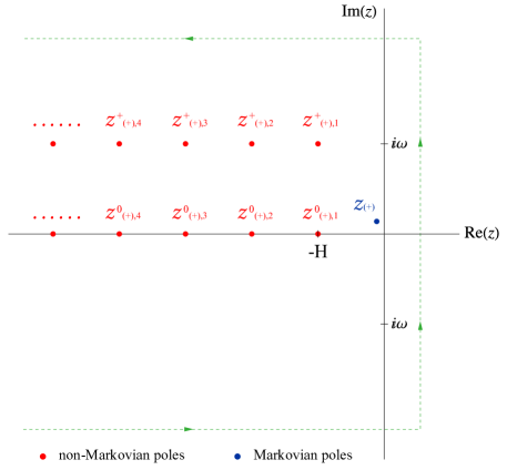
Figure 2: The pole structure of the Laplace-transformed non-diagonal coefficient $\tilde{v}_{(+)}(z;\alpha)$, where one blue point represent Markovian poles $z_{(+)}$, and two infinite sets of red points label the non-Markovian poles $z_{(+),n}^{0}$ and $z_{(+),n}^{+}$ ($n\in\mathbb{Z}^{+}$).

The corresponding residues at these poles are calculated as

$$\left\{\begin{aligned} \mathfrak{Res}\left[\tilde{v}_{(+)}(z;\alpha),z_{(+)}\right]&=\left[1-2g^{2}N_{(+)}^{\prime}(0;\alpha)\right]v_{(+)}(0;\alpha)+\mathcal{O}(g^{4}),\\ \mathfrak{Res}\left[\tilde{v}_{(+)}(z;\alpha),z_{(+),n}^{0}\right]&=-\frac{2g^{2}\;\mathfrak{N}_{n}\;v_{(+)}(0;\alpha)}{n^{2}H^{2}}+\mathcal{O}(g^{4}),\\ \mathfrak{Res}\left[\tilde{v}_{(+)}(z;\alpha),z_{(+),n}^{+}\right]&=-\frac{2g^{2}\;\mathfrak{N}_{n}\;v_{(+)}(0;\alpha)}{(nH-i\omega)^{2}}+\mathcal{O}(g^{4}).\end{aligned}\right.$$ (60)

Summing up all contributions from (60) and using (33), we obtain the off-diagonal part of detector state as (neglecting $\mathcal{O}(g^{4})$ contributions)

$$v_{(\pm)}(\tau;\alpha) \equiv v_{(\pm)}^{\text{Markovian}}+v_{(\pm)}^{\text{non-Markovian}}$$ (61)

$$= v_{(\pm)}(0;\alpha)e^{-\Gamma_{(\pm)}\tau}-g^{2}\bigg{[}S_{(\pm)}(0;\alpha)e^{-\Gamma_{(\pm)}\tau}-S_{(\pm)}(\tau;\alpha)\bigg{]}v_{(\pm)}(0;\alpha).$$

where $\Gamma_{(\pm)}\equiv 2g^{2}N_{(\pm)}(0;\alpha)$ and non-Markovian contribution functions $S_{(\pm)}(\tau;\alpha)$ are defined as

$$S_{\pm}(\tau;\alpha)\equiv-\sum_{n=1}^{\infty}\mathfrak{N}_{n}\left(\frac{1}{n^{2}H^{2}}+\frac{e^{\pm i\omega\tau}}{(nH\mp i\omega)^{2}}\right)e^{-nH\tau}.$$ (62)

Like the structure of (56), the functions $S_{\pm}(\tau;\alpha)$ solely determine all non-Markovian contributions in non-diagonal part of detector state, while the first term of (61) is a part of solution for Markov-approximated master equation.

The functions $S_{(\pm)}(\tau;\alpha)$ and $\Gamma_{(\pm)}$ can be explicitly evaluated as

$$S_{\pm}(\tau;\alpha) =-\frac{1}{\pi^{2}\sinh{\alpha}}\left\{\frac{\cosh{\alpha}}{2}\left[e^{\pm i\omega\tau}\left(\phi\left(e^{-H\tau+i\epsilon},\mp\frac{i\omega}{H}\right)+\phi\left(e^{-H\tau-i\epsilon},\mp\frac{i\omega}{H}\right)\right)\right.\right.$$ (63)

$$- \left.\log\left(2e^{-H\tau}(\cosh{H\tau}-\cos{\epsilon})\right)\bigg{]}+\left[e^{\pm i\omega t}\phi\left(-e^{-H\tau},\mp\frac{i\omega}{H}\right)-\log{\left(1+e^{-H\tau}\right)}\right]\right\},$$

$$\Gamma_{(\pm)} =\frac{\mp i\omega g^{2}}{2\pi^{2}\sinh{\alpha}}\left\{2\cosh{\alpha}\left[\log{(e^{\gamma}\epsilon)}+\psi\left(\mp\frac{i\omega}{H}\right)\right]+\psi\left(\mp\frac{i\omega}{2H}\right)-\psi\left(\frac{H\mp i\omega}{2H}\right)\right\},$$

where $\psi(z)$ is the Digamma function, $\gamma$ is the Euler gamma constant, and all contributions of order $\mathcal{O}(\epsilon\log{\epsilon})$ have been neglected.

We should emphasize that the genuine off-diagonal-decay-rate for detector evolution is the real part of function $\Gamma_{(\pm)}$, which admits a decomposition as

$$\Gamma_{(\pm)}=\left(\frac{\Gamma_{(0)}}{2}-\frac{g^{2}H}{2\pi^{2}}\coth{\frac{\alpha}{2}}\right)\mp\frac{i\Delta\omega}{2},$$ (64)

The so-called Lamb-shifted frequency $\Delta\omega$ can be read from (63):

$$\Delta\omega=\frac{g^{2}\omega}{\pi^{2}\sinh{\alpha}}\left\{2\cosh{\alpha}\left[\log{(e^{\gamma}\epsilon)}+\mathfrak{Re}\;\psi\left(\frac{i\omega}{H}\right)\right]+\mathfrak{Re}\left[\psi\left(\frac{i\omega}{2H}\right)-\psi\left(\frac{{H}+i\omega}{2H}\right)\right]\right\},$$ (65)

which is logarithmic divergent as $\epsilon\rightarrow 0^{+}$.

Moreover, it is interesting to note that $\Gamma_{(0)}$ is of the same order with genuine off-diagonal-decay-rate (the real part in (64)), therefore, we may use $\Gamma_{(0)}$ to encode the collective Markovian-decay-rate for the de Sitter evolution of a comoving UDW detector.

2.4 Markovian v.s. non-Markovian dynamics

We summarize the obtained coefficient functions in Bloch decomposition (12), given by (56) and (61), as

$$\left\{\begin{aligned} v_{(0)}(\tau)&=\gamma_{(0)}\left(e^{-\Gamma_{(0)}\tau}-1\right)+v_{(0)}(0)e^{-\Gamma_{(0)}\tau}-g^{2}\bigg{[}S_{(0)}(0)e^{-\Gamma_{(0)}\tau}-S_{(0)}(\tau)\bigg{]}v_{(0)}(0),\\ v_{(\pm)}(\tau)&=v_{(\pm)}(0)e^{-\Gamma_{(\pm)}\tau}-g^{2}\bigg{[}S_{(\pm)}(0)e^{-\Gamma_{(\pm)}\tau}-S_{(\pm)}(\tau)\bigg{]}v_{(\pm)}(0).\end{aligned}\right.$$ (66)

Before employing quantum Fisher information as a quantitative probe, at present stage, we investigate some qualitative differences between the Markovian and non-Markovian dynamics in the time-evolution (66) of the comoving detector.

Whenever the typical time scale of the environment is much smaller than that of the detector, we can assume the detector undergo a Markovian evolution. By the formulation of (66), this means that we can neglect all terms including non-Markovian contribution functions $S_{(\mu)}$, leading to

$$\left\{\begin{aligned} v_{(0)}(\tau)&=\gamma_{(0)}\left(e^{-\Gamma_{(0)}\tau}-1\right)+v_{(0)}(0)e^{-\Gamma_{(0)}\tau},\\ v_{(\pm)}(\tau)&=v_{(\pm)}(0)e^{-\Gamma_{(\pm)}\tau}.\end{aligned}\right.$$ (67)

The solution satisfies a local Gorini-Kossakowski-Sudarshan-Lindblad (GKSL) master equation Open1 , which is a completely positive and trace-preserving (CPTP) map recasted from (6) via Markov approximation. It is important to note that after sufficient long time, the decay rates $\Gamma_{(\mu)}$ drive the Bloch vector to asymptotic values. The UDW detector thus reach a unique asymptotic state

$$\rho(\tau\rightarrow{\infty})=\frac{1}{2}\begin{bmatrix}1-\gamma_{(0)}&&0\\ 0&&1+\gamma_{(0)}\end{bmatrix}\equiv\frac{e^{-H_{\text{detector }}/T_{\mathrm{eff}}}}{\operatorname{Tr}\left[e^{-H_{\text{detector }}/T_{\mathrm{eff}}}\right]}.$$ (68)

which has a Gibbs form with an effective temperature $T_{\mathrm{eff}}$, and is irrelevant to detector initial states. In the context of black hole background or for an accelerating detector, (68) indicates an inevitable thermalization UDW8 of the UDW detector ending at the equilibrium with Hawking-Unruh temperature Open1-1 ; Open1-2 . However, the de Sitter story is more involved. By substituting the coefficients (48) into (68), we obtain

$$\rho(\tau\rightarrow{\infty})=\frac{1}{2}\begin{bmatrix}\frac{1+\cosh\left(\alpha+\frac{\pi\omega}{H}\right)}{1+\cosh{\alpha}\cosh{\left(\frac{\pi\omega}{H}\right)}}&&0\\ 0&&\frac{1+\cosh\left(\alpha-\frac{\pi\omega}{H}\right)}{1+\cosh{\alpha}\cosh{\left(\frac{\pi\omega}{H}\right)}}\end{bmatrix}+\mathcal{O}(\epsilon\log{\epsilon}),$$ (69)

which means that a comoving UDW detector must approach a thermal state at Gibbons-Hawking temperature $T_{\mathrm{eff}}\equiv T_{GH}=H/2\pi$, once it is asymptotically equilibrium with background fields respecting Bunch-Davies vacuum Open1-3 . However, for general $\alpha-$vacua, even in the equilibrium state (69), we cannot conclude that the detector state is thermal in nature since it fails to satisfy detailed balance condition dS4 . Nevertheless, in a unified perspective from quantum thermodynamics, we can say that the equilibrium state (69) is a result of so-called zeroth law of quantum thermodynamics characterized by a relative entropic formulation Feng1 .

From a general open dynamics (66), we can observe that the non-Markovian contributions become more significant at early time, which means $H\tau\lesssim 1$ for de Sitter context. However, during late-time evolution with $H\tau\gg 1$, the non-Markovian contributions can be absorbed into initial state preparation of detector, i.e., every general solution (66) looks like a Markov-type solution for sufficient large $\tau$, except it has altered initial state different from the one for explicit Markovian solution (67).

This claim can be checked by investigating the explicit solutions (56) and (61). The real parts of the non-Markovian poles satisfy

$$\mathfrak{Re}\left[z\right]\sim-nH+\mathcal{O}(g^{2}),\quad n>0.$$ (70)

At late time $H\tau\gg 1$, the non-Markovian contribution scales as $S_{(\mu)}(\tau)\sim\mathcal{O}(e^{-H\tau})$ for $\mu=0,\pm$, which gives

$$\left\{\begin{aligned} v_{(0)}(\tau;\alpha)&=\gamma_{(0)}\left(e^{-\Gamma_{(0)}\tau}-1\right)+\left(\left[1-g^{2}S_{(0)}(0;\alpha)\right]\left.v_{(0)}\right|_{\tau=0}\right)e^{-\Gamma_{(0)}\tau}+g^{2}\mathcal{O}(e^{-H\tau}),\\ v_{(\pm)}(\tau;\alpha)&=\left(\left[1-g^{2}S_{(0)}(0;\alpha)\right]\left.v_{(\pm)}\right|_{\tau=0}\right)e^{-\Gamma_{(\pm)}\tau}+g^{2}\mathcal{O}(e^{-H\tau}).\end{aligned}\right.$$ (71)

If we regard

$$\left.v^{\prime}_{(0)}\right|_{\tau=0} \equiv\left[1-g^{2}S_{(0)}(0;\alpha)\right]\left.v_{(0)}\right|_{\tau=0},$$ (72)

$$\left.v^{\prime}_{(\pm)}\right|_{\tau=0} \equiv\left[1-g^{2}S_{(0)}(0;\alpha)\right]\left.v_{(\pm)}\right|_{\tau=0}.$$

as shifted initial conditions, (71) are in the same form as the Markovian solution (67). Therefore, we refer the detector density matrix corresponding to (71) as a shifted-Markovian solution with altered initial conditions $v_{(0)}^{\prime}(0)$ and $v_{(\pm)}^{\prime}(0)$. Since $\mathfrak{Re}\left[S_{(\mu)}(0)\right]>0$ by positivity, one notes that $|v_{(\mu)}^{\prime}(0)|<|v_{(\mu)}(0)|$, which is useful for numerical analysis.

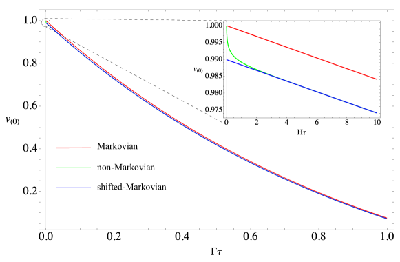
Figure 3: The early- and late-time behaviors of $v_{(0)}(\tau)$ for Markovian, non-Markovian and Shifted Markovian solutions. The detector evolution starts from $\rho(0)=|1\rangle\langle 1|$, with $g=0.1$, $\omega=1$, $H=2\pi$, and the background are chosen as in Bunch-Davies vacuum, i.e., $\alpha\rightarrow-\infty$.

In Figure 3, we illustrate the evolution of the diagonal part of detector density matrix, say $v_{(0)}=\rho_{11}-\rho_{00}$, undergone either Markovian or non-Markovian evolutions. One can observe that the difference between two types of dynamics mainly appears at early time of the detector evolution (depicted in the inset of Fig. 3). As time growing, the non-Markovian contributions decay rapidly for $H\tau\lesssim 1$, and approaches the Shifted Markovian solution for $H\tau\gg 1$, which decays exponentially for large $\tau$.

Finally, we would like to further investigate that how the spacetime geometry (Hubble parameter $H$) and vacuum-choices (superselection parameter $\alpha$) would invoke the difference between Markovian, non-Markovian and Shifted Markovian solutions for the UDW detector. In Figure 4(a), the early-time behavior of $v_{(0)}$ within chosen Bunch-Davies vacuum has been estimated for specific values of Hubble parameter ($H=2\pi,5\pi,15\pi$). We observe that with growing Hubble parameter, the difference between Markovian, non-Markovian and shifted-Markovian solutions decreases. With in mind that the comoving detector in de Sitter should be immersed in a Gibbons-Hawking radiation at temperature $T_{GH}=H/2\pi$, we suggest that the initial difference between three dynamics has been smoothed out by a hotter environment bath.

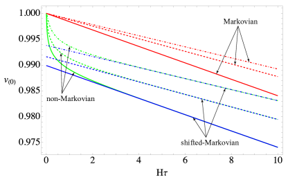
(a) $H=2\pi\ \text{(solid)},5\pi\ \text{(dashed)},15\pi\ \text{(dash-dotted)}$

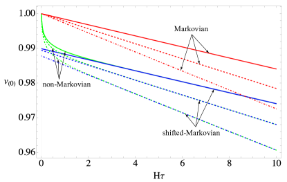
(b) $\alpha=-\infty\ \text{(solid)},-2\ \text{(dashed)},-1\ \text{(dash-dotted)}$

Figure 4: The early-time behavior of $v_{(0)}(\tau)$ for Markovian, non-Markovian and shifted-Markovian solutions. The detector starts from initial state $\rho(0)=|1\rangle\langle 1|$, with $g=0.1$, $\omega=1$. In (a), Hubble parameter is valued as $H=2\pi$ (solid lines), $5\pi$ (dashed lines), and $15\pi$ (dash-dotted lines), which Bunch-Davies vacuum has been chosen, i.e., $\alpha\rightarrow-\infty$. With larger Hubble parameter or Gibbons-Hawking temperature, the difference between three solutions decreases. In (b), the calculation is made with fixed Hubble parameter $H=2\pi$ but for different de Sitter vacua, e.g., $\alpha=-\infty$ (solid lines), $-2$ (dashed lines), and $-1$ (dash-dotted lines). With larger deviation from Bunch-Davies vacuum, the difference between three solutions increases.

In Figure 4(b), similar calculation of $v_{(0)}$ has been taken with fixed Hubble parameter $H=2\pi$ but for general de Sitter $\alpha-$vacua. We note that with larger deviation from Bunch-Davies choice ($\alpha=-\infty$), the initial difference between Markovian and shifted-Markovian solutions increases significantly. In other word, within non-Bunch-Davies vacua in de Sitter, the non-Markovianity of detector evolution is enhanced. Nevertheless, this may not be so surprising if we admire the suggested role played by general $\alpha-$vacua in quantum gravity context dS8+ . That is the superselection parameter $\alpha$ can somehow be related to a minimal-length $e^{\alpha}\sim H/\Lambda$ where fundamental new physics may emerge. Certainly, the Markovian approximation should not be reliable anymore in such extreme case NonM1 .

3 Quantum Fisher information of a comoving UDW detector

As aforementioned, to fully describe the thermalization process of the comoving UDW detector, we need employ some efficient process functions. We choose quantum Fisher information, a crucial concept in quantum metrology and information geometry QFI1-4 ; QFI1-5 . The aim of this section is to explore the QFI of detector’s non-Markovian evolution given by (12) and (66), while the Hubble parameter $H$ serves as the parameter to be optimally estimated. We concern that how the non-Markovian contribution and the influence from general de Sitter vacuum-choices can be recognized from QFI, especially from its early-time behavior as implied by the results of Section 2.4. Within a metrological task on estimating spacetime geometry Open8-5 , QFI bounds the maximal precision of any estimator. Therefore, it is also interesting to investigate that how to effectively enhance the QFI by designing an UDW detector, e.g., carefully selection of its initial state, level spacing, etc. Finally, as the equilibrium state (68) depends solely on Gibbons-Hawking temperature and vacuum-choices $\alpha$, we would naturally expect that asymptotic behavior of QFI should manifest the thermal nature of de Sitter space.

3.1 Definitions and properties

Quantum Fisher information (QFI) is related to the parameter estimating problem in quantum metrology QFI1-1 ; QFI1-2 ; QFI1-3 . Classically, for a $F$-valued random variable $R_{X}:\Omega\rightarrow F$ that depends on a real parameter $X\in\mathbb{R}$, the parameter estimating problem discusses the estimation of $X$ through measuring $R_{X}$. An estimator for sample size $N$ is a map $\hat{X}:F^{N}\rightarrow\mathbb{R}$, which estimates $X$ based on the results of measuring $R_{X}$ for $N$ times. The estimator is unbiased if $E[\hat{X}]=X$. For the random variable $R_{X}$, the classical Fisher information is defined as

$$\mathcal{F}_{C}(X)\equiv\int\mathrm{d}s\,p(s;X)\left(\frac{\partial\log{p(s;X)}}{\partial X}\right)^{2}.$$ (73)

For an unbiased estimator $\hat{X}$ with sample size $N$, the Cramér-Rao bound

$$\mathrm{Var}(\hat{X})\geq\frac{1}{N\mathcal{F}_{C}(X)},$$ (74)

relates $\mathcal{F}_{C}(X)$ to the variance of the estimator $\hat{X}$. As a result, the classical Fisher information $\mathcal{F}_{C}(X)$ essentially represents the amount of information about $X$ that one may extract through measuring $R_{X}$.

In quantum regime, instead of random variables $R_{X}$, one deal with quantum states $\rho_{X}$. Measuring any observable $\hat{A}$ over the Hilbert space $\mathcal{H}$ generates a parameter dependent random variable $A_{X}$, for which the variance is bounded by (74). Defining operator $L$ over the Hilbert space for which the condition

$$\partial_{X}\rho=\frac{1}{2}\{L,\rho\},$$ (75)

is satisfied. The QFI is defined as

$$\mathcal{F}_{Q}(X)\equiv\mathrm{Tr}[\rho L^{2}].$$ (76)

In terms of eigenvectors and eigenvalues of the density matrix $\rho(X)$, we have QFI1-2 ; QFI1-3

$$\mathcal{F}_{Q}(X)=\sum_{i}\frac{(\partial_{X}\lambda_{i})^{2}}{\lambda_{i}}+\sum_{i,j}\frac{2(\lambda_{i}-\lambda_{j})^{2}}{\lambda_{i}+\lambda_{j}}|\langle\psi_{i},\partial_{X}\psi_{j}\rangle|^{2}.$$ (77)

For any observable $\hat{A}$, we have $\mathcal{F}_{C}(X,A)\leq\mathcal{F}_{Q}(X)$. Therefore, for the quantum estimation problem we have

$$\mathrm{Var}(\hat{X})\geq\frac{1}{N\mathcal{F}_{Q}(X)}.$$ (78)

That is, similar to the role of $\mathcal{F}_{C}(X)$ in classical measurements, $\mathcal{F}_{Q}(X)$ qualifies the amounts of information that we can extract about $X$ by measuring quantum states $\rho_{X}$.

For general Hilbert space, (77) is rather complicated for calculation. However, for $\mathrm{dim}\,\mathcal{H}=2$, the qubit density matrix admits a Bloch decomposition, therefore the related QFI can be given explicitly (e.g., from (11)) as

$$\mathcal{F}_{Q}(X)=\sum_{\mu=0,\pm}\left\{\left[\partial_{X}{v}_{(\mu)}\right]^{2}+\frac{\left({v}_{(\mu)}\partial_{X}{v}_{(\mu)}\right)^{2}}{1-|\vec{v}|^{2}}\right\},$$ (79)

which is more convenient for numerical purposes.

For our aim, we wish to estimate Hubble parameter $H$ which characterizes de Sitter geometry. For a comoving UDW detector undergoes general non-Markovian dynamics, the related QFI $\mathcal{F}_{Q}(H;\alpha)$ can be numerically estimated by substituting (66) into (79), where superselection parameter $\alpha$ labeling different de Sitter vacua.

3.2 QFI for the detector in de Sitter Space

3.2.1 Early-time analysis

We begin by analyzing the early-time behavior of $\mathcal{F}_{Q}(H;\alpha)$. As the natural dimensionless time scale in the short time regime is $H\tau$, we plot $\mathcal{F}_{Q}(H;\alpha)$ with respect to $H\tau$ in Figure 5, where the detector initial state has been set to $\rho(0)=|1\rangle\langle 1|$. We compare the early-time behaviors of QFI related to non-Markovian and Markovian solutions respectively.

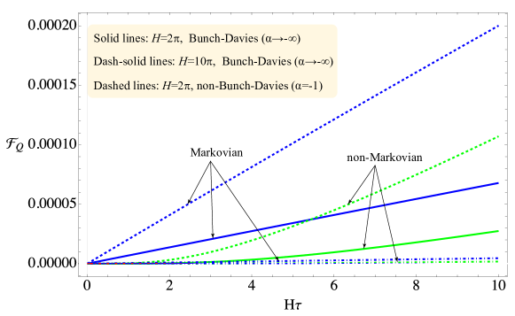
Figure 5: Early-time behavior of $\mathcal{F}_{Q}(H;\alpha)$ for Markovian and non-Markovian solutions. The detector initial condition is $\rho(0)=|1\rangle\langle 1|$, with $g=0.1$, $\omega=1$. For the detector undergoing non-Markovian dynamics, the cooler environment bath and larger deviation from Bunch-Davies vacuum lead to a larger $\mathcal{F}_{Q}(H;\alpha)$ for Hubble parameter estimation.

Firstly, we observe that $\mathcal{F}_{Q}(H;\alpha)$ grows linearly for Markovian solutions, while the growth for non-Markovian solutions is much slower. In particular, we have $\mathcal{F}_{Q}(H;\alpha)\approx 0$ for non-Markovian solutions when $H\tau\lesssim 1$. This is rather general due to the early-time behavior of the correlation function $\Delta^{\pm}(\tau)$. For simplicity we take $\alpha=-\infty$, set $\epsilon^{\prime}:=\epsilon/H$ to be the cutoff with a length/time scale, we have

$$\Delta^{+}(\tau)|_{\alpha=-\infty}=-\frac{H^{2}}{16\pi^{2}\sinh^{2}\big{(}H(\tau-i\epsilon^{\prime})/2\big{)}}=-\frac{1}{4\pi^{2}(\tau-i\epsilon^{\prime})^{2}}(1+O(H^{2}\tau^{2})).$$ (80)

which indicates that for $H\tau\ll 1$, the particle can not distinguish the background from the one in Minkowskian case. Therefore, the exact evolution of the detector at very early time is independent of $H$, and one can not tell any useful information of $H$ from $\rho(\tau)$, i.e., $\mathcal{F}_{Q}(H)$ is almost vanishing. It agrees with the results of non-Markovian solutions. However, when the Markov approximation is performed, the information at early time is lost and we only see a linear growth of $\mathcal{F}_{Q}(H)$. This shows that the Markovian approximation is not reliable at the early-time era of the evolution.

Secondly, we observe that although the QFI related to non-Markovian dynamics is always smaller than that related to Markovian solution, the deviation between them depends on the Hubble parameter $H$ and vacuum-choices $\alpha$. In particular, for larger Hubble parameter $H$ (or higher Gibbons-Hawking temperature $T_{GB}$), the difference between non-Markovian $\mathcal{F}_{Q}(H;\alpha)$ and the one related to Markovian solution degrades, manifesting our previous observation in Figure 4(a) that the different dynamics behave similarly within a hotter environment. On the other hand, for the background field in non-Bunch-Davies vacua, the difference between non-Markovian and Markovian dynamics can be recognized more easily, since the deviation between the related $\mathcal{F}_{Q}(H;\alpha)$ significantly increases as $\alpha\rightarrow 0$. This also validates the result we observed in Figure 4(b).

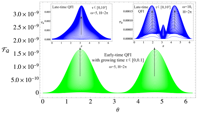
Figure 6: The early and late time behaviors of $\mathcal{F}_{Q}(H;\alpha)$ for arbitrary detector initial states $\rho(0)=|\psi_{\theta}\rangle\langle\psi_{\theta}|$ with $g=0.1$, $H=2\pi$, and $\alpha=-\infty$. Each curves (green or blue) are plotted at specific proper time $\tau$. Along the arrow lines, the time $\tau$ increases monotonously.

From a metrological perspective, we are interested in reaching an optimal measurement accuracy of physical parameter, which is quantified by extreme values of QFI. From Figure 5, for the detector undergoing non-Markovian dynamics, we observe that the cooler environment bath and larger deviation from Bunch-Davies vacuum could lead to a larger $\mathcal{F}_{Q}(H;\alpha)$ for Hubble parameter estimation. Nevertheless, beside its monotonously increasing at early time, to determine the extreme values of $\mathcal{F}_{Q}(H;\alpha)$, we still have to investigate the late-time behavior of QFI for arbitrary initial detector states (say, $|\psi_{\theta}\rangle=\cos{\frac{\theta}{2}}|1\rangle+\sin{\frac{\theta}{2}}|0\rangle$).

For arbitrary detector initial states $\rho(0)=|\psi_{\theta}\rangle\langle\psi_{\theta}|$, we depict both early- and late-time behaviors of $\mathcal{F}_{Q}(H;-\infty)$ in Figure 6. The green curves indicate the early-time QFI which is periodic with $\theta$, and exhibit maximal values for $\theta=(n+1/2)\pi$ ($n\in\mathbb{N}$). Numerically, we confirm that this is a robust and stable pattern for varying $\omega$ or $H$. On the other hand, things get involved at late-time regions. we note that different patterns of QFI curves may exist by tuning $\omega$ and $H$. For example, the left inset of Figure 6 shows a single maximum of QFI curves located for the detector initial state prepared with $\theta=n\pi$, while the right inset with larger $\omega$ shows two maxima of QFI exist.

To end this subsection, we emphasize another important observation from Figure 6. When $\tau$ is sufficiently large, one can recognize that the QFI curves (blue curves in two insets) become intensive and eventually condense to a defined boundary. This means that after sufficient long time, $\mathcal{F}_{Q}(H;\alpha)$ for arbitrary $\omega$ and $H$ would approach asymptotically to a fixed value. This indeed justifies that the comoving UDW detector in de Sitter should approach an unique equilibrium state, which corresponds to a fixed QFI.

3.2.2 Late-time analysis

In this section we further explore the late-time behavior of $\mathcal{F}_{Q}(H;\alpha)$. Since it exhibit an unique asymptotic value for sufficiently late time, we are interested in how the detector approach this thermalization end, as demonstrated by the time-evolution of $\mathcal{F}_{Q}(H;\alpha)$. In other word, the core issue of this section is to use $\mathcal{F}_{Q}(H;\alpha)$ for distinguishing various thermalization paths in detector Hilbert space to an unique end.

We start by working with a detector in Bunch-Davies vacuum. For fixed Hubble parameter, the related QFI $\mathcal{F}_{Q}(H;-\infty)$ is determined by the delicate design of detector, i.e., energy spacing $\omega$ and initial state preparation $\theta$. In Figure 7, we show the behaviors of $\mathcal{F}_{Q}(H;-\infty)$ for various choices of $\omega$ and $\theta$, while the time evolution under non-Markovian (Markovian) dynamics is depicted by solid (dashed) lines. The sub-figures in Figure 7 corresponds to specific designed energy spacing $\omega=0.25,1,3,6,10,15$, while the colored $\mathcal{F}_{Q}(H;-\infty)$ curves in each sub-figure determined by different initial states $\theta=0,\pi/4,\pi/2,3\pi/4,\pi$. In this sense, we can say that QFI distinguishes the different thermalization paths of the detector.

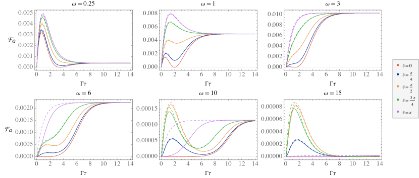
Figure 7: Late-time behavior of $\mathcal{F}_{Q}(H;-\infty)$ for Markovian (dashed lines) and non-Markovian (solid lines) solutions. The numerical analysis is performed for $g=0.1$, $H=2\pi$, with various detector energy spacing ($\omega=0.25,1,3,6,10,15$) and initial states ($\theta=0,\pi/4,\pi/2,3\pi/4,\pi$).

It is obvious that after sufficient long time, the detector QFI under either dynamics will converge to an unique end, which is irrelevant with the initial state preparation $\theta$, and manifests the zeroth law of quantum thermodynamics for the detector thermalization in de Sitter. For fixed Hubble parameter, the specific value of the converging end depends on the detector energy gap $\omega$. One can see that for extremal small or large $\omega$, the QFI $\mathcal{F}_{Q}(H;-\infty)$ asymptotically converges to zero. This can be confirmed from the detector equilibrium state (69) at long-time limit. With Bunch-Davies choice $\alpha=-\infty$, it gives

$$\rho^{BD}_{\text{asym}}{=}\frac{1}{2}\begin{bmatrix}1-\tanh\left(\frac{\pi\omega}{H}\right)&&0\\ 0&&1+\tanh\left(\frac{\pi\omega}{H}\right)\end{bmatrix}.$$ (81)

For extremely small $\omega$, we have a $H$-independent asymptotic state $\rho^{BD}_{\text{asym}}\approx\mathbb{I}/2$, leading to a vanishing QFI for Hubble parameter estimation. On the other hand, for large $\omega$, the density matrix approaches $\rho^{BD}_{\text{asym}}\approx|0\rangle\langle 0|/2$, which is again independent of $H$. In conclusion, the maximal asymptotic QFI can only be achieved for fine-tuned detector energy gap $\omega$, which leads to a final state (81) that acquires most $H$-dependence.

Moreover, we observe from Figure 7 that during the time evolution the QFI related to non-Markovian dynamics is always smaller than the case of Markovian evolution. Recall from section 2.4 that the non-Markovian dynamics resembles a shifted-Markovian solution in late-time regime, therefore the shift of detector initial condition always reduces the coherence of the density matrix.

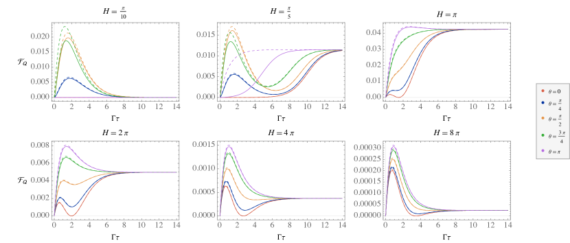
Figure 8: Late-time behavior of $\mathcal{F}_{Q}(H;-\infty)$ for Markovian and non-Markovian solutions. The estimation has been taken under $g=0.1$, $\omega=1$, for various Hubble parameter values (with $H=0.1\pi,0.2\pi,\pi,2\pi,4\pi,8\pi$) and initial states (with $\theta=0,\pi/4,\pi/2,3\pi/4,\pi$).

We now move to the case of the detector with fixed energy gap but estimating varying Hubble parameter. Intuitively, with optimal measurement, it could be easier to measure a large parameter. However, as shown in Figure 8, one can observe that for a large Hubble parameter, the related asymptotic QFI may approach to zero, exhibiting a similar pattern of time evolution just as those shown in Figure 7. This may not be surprised since the Hubble parameter and detector energy gap are always combined as ${\omega}/{H}$ in (81). Nevertheless, with noticing the two-fold role of Hubble parameter, i.e., a parameter to be estimated metrologically as well as determining a Gibbons-Hawking bath, we have a more physical interpretation on the vanishing asymptotic QFI for large $H$, as it means a hotter de Sitter bath disturbing any optimal quantum measurement on the Hubble parameter.

We would like to explore that how the de Sitter vacuum-choices would affect the time-evolution of the QFI for Hubble parameter estimation. The numerical estimation of time evolving $\mathcal{F}_{Q}(H;\alpha)$ is shown in Figure 9. Similar to Bunch-Davies choice, for general $\alpha-$vacua, the QFI $\mathcal{F}_{Q}(H;\alpha)$ undergoing Non-Markovian dynamics keep lower than its Markovian counterpart. Moreover, we observe that for fixed Hubble parameter and detector energy gap, the more deviation of de Sitter vacuum from Bunch-Davies choice, the lower asymptotically converging end of $\mathcal{F}_{Q}(H;\alpha)$ one can obtain. Such suppression can be attributed to the emerging $\alpha-$dependence in the detector equilibrium state (69) for the choices of non-Bunch-Davies vacuum of de Sitter field theory. As $\alpha$ approaches $0^{-}$, we have $\gamma_{(0)}\rightarrow 0$, giving a $H$-independent equilibrium state $\rho^{non-BD}_{\text{asym}}\approx\mathbb{I}/2$, leading to a vanishing asymptotic QFI.

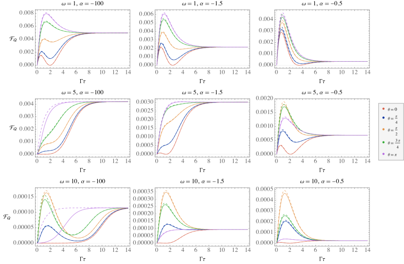
Figure 9: Late-time behavior of $\mathcal{F}_{Q}(H;\alpha)$ for Markovian (dashed lines) and non-Markovian (solid lines) solutions. The estimation has been taken under $g=0.1$, $H=2\pi$, for various de Sitter vacuum-choices ($\alpha=-100,-1.5,-0.5$), detector energy gap (with $\omega=1,5,10$) and initial states (with $\theta=0,\pi/4,\pi/2,3\pi/4,\pi$).

Like in Bunch-Davies case, we can prove the vanishingness of asymptotic $\mathcal{F}_{Q}(H;\alpha)$ also at the limits of extremely small/large detector energy gap. For $\omega\rightarrow 0$, we still obtain the $H$-independent equilibrium state $\rho^{non-BD}_{\text{asym}}\approx\mathbb{I}/2$, giving vanishing $\mathcal{F}_{Q}(H;\alpha)$. For large $\omega$, we obtain

$$\lim_{\omega\rightarrow\infty}\gamma_{(0)}=\lim_{\omega\rightarrow\infty}-\frac{\sinh{\alpha}\sinh{\left(\frac{\pi\omega}{H}\right)}}{1+\cosh{\alpha}\cosh{\left(\frac{\pi\omega}{H}\right)}}=-\tanh{\alpha},$$ (82)

which turns the detector equilibrium state (69) into

$$\rho^{non-BD}_{\text{asym}}=\frac{1}{2}\begin{bmatrix}1+\tanh{\alpha}&&0\\ 0&&1-\tanh{\alpha}\end{bmatrix}.$$ (83)

This is an asymptotic state independent of the Hubble parameter, leading to vanishing QFI.

We end this section with an interpretation of (83). For the detector initially at ground state, it requires amount of energy $\Delta E=\hbar\omega$ to be excited to higher level. For Bunch-Davies vacuum, we know that the detector eventually arrives the equilibrium state $\rho^{BD}_{\text{asym}}\approx|0\rangle\langle 0|/2$ once $\omega\rightarrow\infty$. This is reasonable since the de Sitter thermal bath at finite-temperature $T_{BD}=H/2\pi$ can not provide enough energy to excite the detector. However, for general $\alpha$-vacua, (83) indicates that the detector can be excited from ground state $|0\rangle$ even when an infinite excitation energy $\Delta E\gg 0$ is required. The only possibility this can happen is that the background field states $|\alpha\rangle$ should have infinite energy dS4 ; alpha-1 . Historically, this phenomenon caused years’ debate on the pathological nature of $\alpha-$states in a realistic cosmology alpha-2 . Nevertheless, it is interesting to note that such argued pathology has never been diagnosed by QFI as we did.

4 Conclusions

In this work, we have resolved the non-Markovian dynamics of a comoving UDW detector in de Sitter space. In terms of quantum Fisher information of Hubble parameter estimation, we found that the non-Markovian contribution is very robust and stable at early time. At late time, we shown that the non-Markovian effect in general reduces the QFI, which converges to an asymptotic value independent on detector’s initial state preparation. Moreover, we are particularly interested in the influence of de Sitter $\alpha$-vacuum choices on detector dynamics, manifested by related QFI. For general $\alpha$-vacua, we found that the asymptotic values of QFI can significantly be suppressed, comparing to the case of Bunch-Davies vacuum.

The method adopted in the paper can be generalized to other important spacetime geometries, such as black hole Open1-5 or FRW universe. The related QFI is then anticipated to play a similar role on characterizing detector dynamics, as well as specific features of quantum fields in curved background. On the other hand, once be generalized to multi-parameters $X_{i}$ estimation, the related QFI matrix $\mathcal{F}_{ij}$ can be identified as a metric in state space, from a information geometric perspective. It is related to many important concepts in quantum thermodynamics QFI1-4 ; QFI1-5 , e.g., relative entropy as $\mathcal{F}_{ij}=\partial^{2}D(\mathbf{X}|\mathbf{X}^{\prime})/\partial X_{i}\partial X_{j}$. We expect that such link can be manifested in future through a discussion on the quantum thermodynamics of UDW detector Feng1 in de Sitter space.

Appendix A Solving the Laplace-transformed master equation

In Section 2.1, we obtained the Laplace-transformed non-Markovian master equation (13)

$$z\tilde{\rho}(z)-\rho(0)=g^{2}\sum_{\mu=0,\pm}\int_{0}^{\tau}ds\,[\sigma^{(\mu)}\tilde{\rho}(z),\sigma^{{\dagger}}_{(\mu)}]\tilde{\Delta}^{+}(z+i\mu\omega)+h.c.$$ (84)

From the decomposition $\rho=\frac{1}{2}(1+\sum_{\mu}v_{(\mu)}\sigma^{(\mu)})$, we have

$$\tilde{\rho}=\frac{1}{2}\left(\frac{1}{z}+\sum_{\mu}\tilde{v}_{(\mu)}\sigma^{(\mu)}\right).$$ (85)

which further gives

$$\left[\sigma^{(\mu)}\tilde{\rho}(z),\sigma^{{\dagger}}_{(\mu)}\right]=\frac{1}{2}\left(\frac{1}{z}[\sigma^{(\mu)},\sigma^{{\dagger}}_{(\mu)}]+\sum_{\nu}\tilde{v}_{(\nu)}[\sigma^{(\mu)}\sigma^{(\nu)},\sigma^{{\dagger}}_{(\mu)}]\right).$$ (86)

Using (7), we know that

$$\left[\sigma^{(\mu)},\sigma^{(\nu)}\right]=-2\sum_{\gamma}\epsilon^{\mu\nu\gamma}\sigma^{{\dagger}}_{\gamma},~{}~{}~{}~{}~{}~{}\left\{\sigma^{(\mu)},\sigma^{{\dagger}}_{(\nu)}\right\}=2\delta^{\mu}_{\,\nu}$$ (87)

which leads

$$\left[\sigma^{(\mu)}\tilde{\rho}(z),\sigma^{{\dagger}}_{(\mu)}\right]=\frac{\mu\sigma^{(0)}}{z}-\sum_{\nu\neq\mu}\tilde{v}_{(\nu)}\sigma^{(\nu)}.$$ (88)

Substituting it back in the Laplace-transformed Master equation (86), one obtains

$$z\tilde{\rho}(z)-\rho(0)=g^{2}\left(M(z)\sigma^{(0)}/z-\sum_{\nu=0,\pm}N_{(\nu)}(z)\tilde{v}_{(\nu)}\sigma^{(\nu)}\right),$$ (89)

where

$$N_{(\nu)}(z)\equiv\sum_{\mu\neq\nu}[\tilde{\Delta}^{+}(z+i\mu\omega)+\tilde{\Delta}^{-}(z+i\mu\omega)],$$ (90)

$$M(z)\equiv\tilde{\Delta}^{+}(z+i\omega)+\tilde{\Delta}^{-}(z-i\omega)-\tilde{\Delta}^{+}(z-i\omega)-\tilde{\Delta}^{-}(z+i\omega).$$

Noticing that

$$z\tilde{\rho}-\rho(0)=\sum_{\mu=0,\pm}\frac{1}{2}\left[z\tilde{v}_{(\mu)}-v_{(\mu)}(0)\right]\sigma^{(\mu)},$$ (91)

and comparing its coefficients before $\sigma^{(\mu)}$ with (89), we obtain the solutions (15).

Appendix B Laplace transform of the correlation functions

In Section 2.2 we defined the functions $E_{(\pm)}(z)$ and $F(z)$. We start from calculation of $E_{(+)}(z)$:

$$E_{(+)}(z)=-\int_{0}^{\infty}\mathrm{d}\tau\,\frac{e^{-z\tau}}{16\pi^{2}\sinh^{2}((H\tau-i\epsilon)/2)}.$$ (92)

Applying integration by parts to the denominator, we obtain

$$E_{(+)}(z)=\frac{H}{8\pi^{2}}\left(\coth{\frac{i\epsilon}{2}}+\int_{0}^{\infty}\,\mathrm{d}\tau\,ze^{-z\tau}\coth{\frac{H\tau-i\epsilon}{2}}\right).$$ (93)

Changing the integration variable to $u\equiv e^{-H\tau}$, and expanding $\coth{\frac{H\tau-i\epsilon}{2}}$ as a power series in $u$, we get

$$E_{(+)}(z)=\frac{H}{8\pi^{2}}\left(\pm\coth{\frac{i\epsilon}{2}}+2z\sum_{n=0}^{\infty}\frac{e^{\pm in\epsilon}}{z+nH}-1\right),$$ (94)

from which $E^{-}(p)$ can also be determined by the substitution $\epsilon\rightarrow-\epsilon$.

In a similar way, we evaluate $F(z)$ as

$$F(z)=\frac{H}{8\pi^{2}}\left(2z\sum_{n=0}^{\infty}\frac{(-1)^{n}\cos{n\epsilon}}{z+nH}-1\right).$$ (95)

It is worth mentioning that although (94) contains linearly divergent terms $\pm\coth{\frac{i\epsilon}{2}}$, they are always canceled when we evaluate $M(z)$ and $N_{(\mu)}(z)$. On the other hand, the $e^{\pm in\epsilon}$ factors protect the convergence of (17) in an intricate way, and are therefore more important. To make sure that we do everything correctly, we keep $\epsilon$ to be small but finite throughout all calculation, and only neglect contributions that are guaranteed to be small in the final results $\rho(t)$. In fact, $\epsilon$ is naturally related to the cutoff of the background fields through $\Lambda/H\sim 1/\epsilon$, which is expected to be a small and positive value.

Appendix C Calculation of the constants $\gamma_{(0)}$ and $\Gamma_{(\mu)}$

In this Appendix we aim to calculate the coefficient functions (48) and (63), defined by

$$\gamma_{(0)}=-\frac{M(0)}{N_{0}(0)},~{}~{}~{}~{}~{}~{}\Gamma_{(\mu)}=2g^{2}N_{(\mu)}(0),~{}~{}~{}~{}~{}\mu=0,\pm$$ (96)

From (16), we know that

$$M(0;\alpha) =\tilde{\Delta}^{+}(i\omega;\alpha)+\tilde{\Delta}^{-}(-i\omega;\alpha)-\tilde{\Delta}^{+}(-i\omega;\alpha)-\tilde{\Delta}^{-}(i\omega;\alpha),$$ (97)

$$N_{(0)}(0;\alpha) =\tilde{\Delta}^{+}(i\omega;\alpha)+\tilde{\Delta}^{-}(-i\omega;\alpha)+\tilde{\Delta}^{+}(-i\omega;\alpha)+\tilde{\Delta}^{-}(i\omega;\alpha),$$

$$N_{(\pm)}(0;\alpha) =\tilde{\Delta}^{+}(\mp i\omega;\alpha)+\tilde{\Delta}^{-}(\mp i\omega;\alpha)+\tilde{\Delta}^{+}(0;\alpha)+\tilde{\Delta}^{-}(0;\alpha)$$

Introducing the Fourier-transformed Wightman function $\mathcal{G}(\omega)\equiv\int\mathrm{d}\tau\,e^{i\omega\tau}\Delta^{+}(\tau)$, above coefficient functions can be recasted into

$$M(0;\alpha) =\mathcal{G}(-\omega)-\mathcal{G}(\omega),$$ (98)

$$N_{(0)}(0;\alpha) =\mathcal{G}(-\omega)+\mathcal{G}(\omega),$$

$$\mathfrak{Re}\left[N_{(\pm)}(0;\alpha)\right] =\mathcal{G}(0)+\frac{\mathcal{G}(-\omega)+\mathcal{G}(\omega)}{2}.$$

The derivation of $\mathcal{G}(\omega)$ in de Sitter space is standard and straightforwardly dS12-2 ; dS10 , by which the coefficient functions become

$$M(0;\alpha) =-\frac{\omega}{2\pi}+\mathcal{O}(\epsilon\log{\epsilon}),$$ (99)

$$N_{(0)}(0;\alpha) =-\left(\frac{\omega}{2\pi}\right)\frac{1+\cosh{\alpha}\cosh{\left(\frac{\pi\omega}{H}\right)}}{\sinh{\alpha}\sinh{\left(\frac{\pi\omega}{H}\right)}}+\mathcal{O}(\epsilon\log{\epsilon}),$$

where the $\mathcal{O}(\epsilon\log{\epsilon})$ term can be estimated through the condition

$$\sum_{n>0}\frac{|\sin{n\epsilon}|}{n^{2}}\sim\mathcal{O}(\epsilon\log{\epsilon}),$$ (100)

which would be proved later in Appendix D. Substituting (99) into (96), we obtain

$$\gamma_{(0)} =-\frac{\sinh{\alpha}\sinh{\left(\frac{\pi\omega}{H}\right)}}{1+\cosh{\alpha}\cosh{\left(\frac{\pi\omega}{H}\right)}}+\mathcal{O}(\epsilon\log{\epsilon}),$$ (101)

$$\Gamma_{(0)} =-\left(\frac{g^{2}\omega}{\pi}\right)\frac{1+\cosh{\alpha}\cosh{\left(\frac{\pi\omega}{H}\right)}}{\sinh{\alpha}\sinh{\left(\frac{\pi\omega}{H}\right)}}+\mathcal{O}(g^{2}\epsilon\log{\epsilon}).$$

which is (48) as we expected.

To calculate $\Gamma_{(\pm)}$, while its real part is easy to get as $\mathfrak{Re}\left[\Gamma_{(\pm)}\right]=2g^{2}\mathfrak{Re}\left[N_{(\pm)}(0;\alpha)\right]$, we need a bit more effort to derive its imaginary part. Based on (97), (21) and (23), we have

$$N_{(\pm)}(0;\alpha)=\pm\frac{i\omega}{2\pi^{2}}\left(\coth{\alpha}\sum_{n=0}^{\infty}\frac{\cos{n\epsilon}}{nH\mp i\omega}+\operatorname{csch}{\alpha}\sum_{n=0}^{\infty}\frac{(-1)^{n}\cos{n\epsilon}}{nH\mp i\omega}\right).$$ (102)

Noting that

$$\sum_{n=0}^{\infty}\frac{\cos{n\epsilon}}{nH\mp i\omega}=-\frac{1}{H}\left(\log{\epsilon}+\psi\left(\mp\frac{i\omega}{H}\right)+\gamma\right)+\mathcal{O}(\epsilon\log{\epsilon}),$$ (103)

and

$$\sum_{n=0}^{\infty}\frac{(-1)^{n}\cos{n\epsilon}}{nH-i\omega}=-\frac{1}{2H}\left(\psi\left(\frac{i\omega}{2H}\right)-\psi\left(1+\frac{i\omega}{2H}\right)\right)+\mathcal{O}(\epsilon\log{\epsilon}),$$ (104)

we eventually obtain (63).

Appendix D Calculation of the inhomogeneous non-Markovian contributions

In section 2.3.1, we considered the non-Markovian inhomogeneous contribution controlled by the estimator (54), which is

$$\mathfrak{E}(\tau)=\frac{i}{\pi^{2}}\sum_{n>0}n\sin{n\epsilon}\left(\frac{e^{i\omega\tau-nH\tau}}{(n-i\omega/H)^{2}}-\frac{e^{-i\omega\tau-nH\tau}}{(n+i\omega/H)^{2}}\right),$$ (105)

Setting $H=1$ for simplicity and expanding $e^{i\omega\tau}$, we get:

$$\mathfrak{E}(\tau)=-\frac{2}{\pi^{2}}\sum_{n>0}\sin{n\epsilon}\left(\frac{2n^{2}\omega e^{-n\tau}\cos{\omega\tau}+(n^{2}-\omega^{2})ne^{-n\tau}\sin{\omega\tau}}{(n^{2}+\omega^{2})^{2}}\right).$$ (106)

For $\tau\in[0,\infty)$ and $|\sin{\omega\tau}|\leq\omega\tau$, the following inequality holds

$$|ne^{-n\tau}\sin{\omega\tau}|\leq n\omega\tau e^{-n\tau}\leq\omega.$$ (107)

which with a little bit of algebra, gives

$$|\mathfrak{E}(\tau)|\leq\frac{8\omega}{\pi^{2}}\sum_{n>0}\frac{|\sin{n\epsilon}|}{n^{2}}$$ (108)

For given positive number $N>1$, we have

$$\left|\mathfrak{E}(\tau)\right|\leq\frac{8\omega}{\pi^{2}}\left(\sum_{n=1}^{N}\frac{|\sin{n\epsilon}|}{n^{2}}+\sum_{n=N+1}^{\infty}\frac{1}{n^{2}}\right).$$ (109)

Using the fact that $|\sin{n\epsilon}|<n\epsilon$ for $n>0$, we must have

$$|\mathfrak{E}(\tau)|\leq\frac{8\omega}{\pi^{2}}\left(\epsilon(1+\log{N})+\frac{1}{N}\right).$$ (110)

Choosing $N=\lceil 1/\epsilon\rceil$, we eventually have

$$|\mathfrak{E}(\tau)|\leq\frac{8\omega\epsilon\left(3-\log{\epsilon}\right)}{\pi^{2}},$$ (111)

which justifies our assertion that $f(\tau)\sim O(\epsilon\log{\epsilon})$ used in Section 2.3.1.

References

- (1) D. Anninos, De Sitter musings, Int. J. Mod. Phys. A 27, 1230013 (2012).
- (2) E. Witten, Quantum Gravity In De Sitter Space, arXiv:hep-th/0106109.
- (3) W. G. Unruh, Notes on black-hole evaporation, Phys. Rev. D 14, 870 (1976).
- (4) B. S. DeWitt, Quantum gravity: the new synthesis, in General Relativity: An Einstein Centenary Survey, edited by S.W. Hawking and W. Israel (Cambridge University Press, Cambridge, 1979), pp. 680.
- (5) N. D. Birrell and P. C. W. Davies, Quantum fields in curved space, Cambridge University Press (1982).
- (6) L. C. B. Crispino, A. Higuchi and G. E. A. Matsas, The Unruh effect and its applications, Rev. Mod. Phys. 80, 787 (2008).
- (7) P. Candelas, Vacuum polarization in Schwarzschild spacetime, Phys. Rev. D 21, 2185 (1980).
- (8) S. W. Hawking, Particle creation by black holes, Commun. Math. Phys. 43, 199 (1975).
- (9) G. W. Gibbons and S. W. Hawking, Cosmological event horizons, thermodynamics, and particle creation, Phys. Rev. D 15, 2738 (1977).
- (10) B. Garbrecht and T. Prokopec, Unruh response functions for scalar fields in de Sitter space, Class. Quant. Grav. 21, 4993 (2004).
- (11) G. L. Sewell, Quantum fields on manifolds: PCT and gravitationally induced thermal states, Ann. Phys. 141, 201 (1982).
- (12) S. Takagi, Vacuum Noise and Stress Induced by Uniform Acceleration, Prog. Theor. Phys. Suppl. 88, 1 (1986).
- (13) J. Arrechea, C. Barceló, L. J. Garay, and G. García-Moreno, Inversion of statistics and thermalization in the Unruh effect, Phys. Rev. D 104, 065004 (2021).
- (14) F. Benatti and R. Floreanini, Entanglement generation in uniformly accelerating atoms: reexamination of the Unruh effect, Phys. Rev. A 70, 012112 (2004).
- (15) H. Yu and J. Zhang, Understanding Hawking radiation in the framework of open quantum systems, Phys. Rev. D 77, 024031 (2008).
- (16) H. Yu, Open quantum system approach to Gibbons-Hawking effect of de Sitter space-time, Phys. Rev. Lett. 106, 061101 (2011).
- (17) G. Kaplanek and C.P. Burgess, Hot accelerated qubits: decoherence, thermalization, secular growth and reliable late-time predictions, J. High Energy Phys. 03 (2020) 008.
- (18) G. Kaplanek and C.P. Burgess, Qubits on the horizon: decoherence and thermalization near black holes, J. High Energy Phys. 01 (2021) 098.
- (19) J. Feng, Y. -Z. Zhang, M. D. Gould, and H. Fan, Uncertainty relation in Schwarzschild spacetime, Phys. Lett. B 743, 198 (2015).
- (20) L. Jia, Z. Tian, and J. Jing, Entropic uncertainty relation in de Sitter space, Ann. Phys. 353, 37 (2015).
- (21) J. Hu and H. Yu, Geometric phase outside a Schwarzschild black hole and the Hawking effect, J. High Energy Phys. 09 (2012) 062.
- (22) Z. Tian and J. Jing, Geometric phase of two-level atoms and thermal nature of de Sitter spacetime, J. High Energy Phys. 04 (2013) 109.
- (23) J. Feng, J.-J. Zhang, and Y. Zhou, Thermality of the Unruh effect with intermediate statistics, Europhys. Lett. 137, 60001 (2022).
- (24) S.-W. Han, Z. Ouyang, Z. Hu, and J. Feng, Relative entropy formulation of thermalization process in a Schwarzschild spacetime, to appear.
- (25) M. Fukuma, S. Sugishita, and Y. Sakatani, Master equation for the Unruh-DeWitt detector and the universal relaxation time in de Sitter space, Phys. Rev. D 89, 064024 (2014).
- (26) G. Kaplanek and C.P. Burgess, Hot cosmic qubits: late-time de Sitter evolution and critical slowing down, J. High Energ. Phys 02 (2020) 053.
- (27) C.P. Burgess, R. Holman, G. Kaplanek, J. Marting and V. Vennin, Minimal decoherence from inflation, J. Cosmol. Astropart. 07 (2023) 022.
- (28) H. P. Breuer and F. Petruccione, The Theory of Open Quantum Systems (Oxford University Press 2002).
- (29) G. Kaplanek and E. Tjoa, Effective master equations for two accelerated qubits, Phys. Rev. A 107, 012208 (2023).
- (30) D. Moustos and C. Anastopoulos, Non-Markovian time evolution of an accelerated qubit, Phys. Rev. D 95, 025020 (2017).
- (31) D. Moustos, Asymptotic states of accelerated detectors and universality of the Unruh effect, Phys. Rev. D 98, 065006 (2018).
- (32) E. Mottola, Particle creation in de Sitter space, Phys. Rev. D 31, 754 (1985).
- (33) B. Allen, Vacuum states in de Sitter space, Phys. Rev. D 32, 3136 (1985).
- (34) M. B. Einhorn and F. Larsen, Interacting quantum field theory in de Sitter vacua, Phys. Rev. D 67, 024001 (2003).
- (35) K. Goldstein and D. A. Lowe, A note on -vacua and interacting field theory in de Sitter space, Nucl. Phys. B 669, 325 (2003).
- (36) H. Collins, R. Holman, and M. R. Martin, The fate of the alpha-vacuum, Phys. Rev. D 68, 124012 (2003).
- (37) J. de Boer, V. Jejjala, and D. Minic, -states in de Sitter space, Phys. Rev. D 71, 044013 (2005).
- (38) U. H. Danielsson, Inflation, holography, and the choice of vacuum in de Sitter space, J. High Energy Phys. 07 (2002) 040.
- (39) U. H. Danielsson, Note on inflation and trans-Planckian physics, Phys. Rev. D 66, 023511 (2002).
- (40) K. Goldstein and D. A. Lowe, Quantum initial conditions for inflation and canonical invariance, Phys. Rev. D 69, 023507 (2004).
- (41) R. Bousso, A. Maloney and A. Strominger, Conformal vacua and entropy in de Sitter space, Phys. Rev. D 65, 104039 (2002).
- (42) U. Danielsson, The quantum swampland, J. High Energy Phys. 04, 095 (2019).
- (43) M. Aspachs, G. Adesso, and I. Fuentes, Optimal Quantum Estimation of the Unruh-Hawking Effect, Phys. Rev. Lett. 105, 151301 (2010).
- (44) Z. Tian, J. Wang, H. Fan, and J. Jing, Relativistic Quantum Metrology in Open System Dynamics, Sci. Rep. 5, 7946 (2015).
- (45) J. Feng and J.-J. Zhang, Quantum fisher information as a probe for Unruh thermality, Phys. Lett. B 827, 136992 (2022).
- (46) J. Wang, Z. Tian, J. Jing, and H. Fan, Parameter estimation for an expanding universe, Nucl. Phys. B 892, 390 (2015).
- (47) H. Du and R. B. Mann, Fisher information as a probe of spacetime structure: Relativistic quantum metrology in (A)dS, J. High Energ. Phys 05 (2021) 112.
- (48) E. Pattersona and R. B. Mann, Fisher information of a black hole spacetime, J. High Energ. Phys. 06 (2023) 214.
- (49) X. Huang, J. Feng, Y.Z. Zhang, and H. Fan, Quantum estimation in an expanding spacetime, Ann. Phys. 397, 336 (2018).
- (50) E. B. Davies, Markovian Master Equations, Commun. Math. Phys. 39, 91 (1974).
- (51) J. Feng, X. Huang, Y.-Z. Zhang, and H. Fan, Bell inequalities violation within non-Bunch-Davies states, Phys. Lett. B 786, 403 (2018).
- (52) F. W. J. Olver, D. W. Lozier, R. F. Boisvert, and C. W. Clark, NIST Handbook of Mathematical Functions (Cambridge University Press 2010), pp. 612.
- (53) C. W. Helstrom, Quantum detection and estimation theory, J. Stat. Phys. 1, 231 (1969).
- (54) S. L. Braunstein and C. M. Caves, Statistical distance and the geometry of quantum states, Phys. Rev. Lett. 72, 3439 (1994).
- (55) M. G. A. Paris, Quantum estimation for quantum technology, Int. J. Quantum Inf. 7, 125 (2009).
- (56) G. B. Arfken and H. J. Weber, Mathematical Methods for Physicists, 6th Edition (Academic Press 2005).
- (57) S.-W. Han, Z. Ouyang, Z. Hu, and J. Feng, Relative entropy formulation of thermalization process in a Schwarzschild spacetime, to appear.
- (58) H. P. Breuer, E. Laine, J. Piilo, and B. Vacchini, Non-Markovian dynamics in open quantum systems, Rev. Mod. Phys. 88, 021002 (2016).
- (59) J. S. Sidhu and P. Kok, Geometric perspective on quantum parameter estimation, AVS Quantum Sci. 2, 014701 (2020).
- (60) J. Lambert and E. S. Sørensen, From classical to quantum information geometry: a guide for physicists, New J. Phys. 25, 081201 (2023).
- (61) N. Kaloper, M. Kleban, A. Lawrence, S. Shenker and L. Susskind, Initial conditions for inflation, J. High Energy Phys. 11, 037 (2002).
- (62) U. Danielsson, On the consistency of de Sitter vacua, J. High Energy Phys. 12, 025 (2012).