Harris Dispersion Relation and Bernstein Modes in Dense Magnetized Quantum Plasmas

Abstract

The Bernstein wave is a well-known electrostatic eigen-mode in magnetized plasmas, and it is of broad connection to multiple disciplines, such as controlled nuclear fusions and astrophysics. In this work, we extend the Bernstein mode from classical to quantum plasmas by means of the quantum kinetic theory in a self-consistent manner, and especially the quantum version of the Harris dispersion relation is derived. The studied quantum effects appear in the form of pseudo-differential operators (ΨDO) in the formula, which are exactly solved using numerical methods. Furthermore, by utilizing the magnetized equilibrium Wigner function, Landau quantization and finite temperature effects are rigorously contained. It is found that behaviours of the quantum Bernstein wave departure significantly from its classical counterpart, especially when $\hbar\omega_{\mathrm{c}}$ is of the same order of the Fermi energy.

I Introduction

Bernstein modes are electrostatic eigen-modes of a magnetized plasma, first discovered by I.B. Bernstein in 1958 [1]. Some authors [2, 3, 4] refer to a Bernstein mode as a “magnetoplasmon”, since the electrostatic eigen-mode of a unmagnetized plasma, i.e., the Langmuir wave, is often referred to as a “plasmon”. Bernstein modes has drawn wide interest from multiple academic discipline. For example, electron or ion Bernstein modes serve as an effective heating mechanism in magnetic confined fusion researches [5, 6, 7, 8]. In solid-state physics, magnetoplasmons in a 2D electron gas are a very important topic related to semiconductor devices and quantum Hall effect [9, 10, 11]. Further more, Bernstein modes are also of interest in the fields of space plasmas [12, 13, 14, 15] and strong coupling plasmas [16, 17, 18].

The main objective of this paper is to extend the linear analysis of Bernstein modes from classical plasmas to quantum plasmas. In this context, quantum plasma refers to a plasma where the electron density is sufficiently high that the thermal de Broglie wavelength of electrons becomes comparable to the average distance between them, or where the energy of a plasmon is comparable to the thermal/Fermi energy. Quantum plasmas are ubiquitous in the universe, for example, white dwarfs and other old or dead stars contain a significant amount of quantum plasmas. Some models used to explain certain high-energy astrophysical phenomena (such as X- or $\gamma$-ray bursts) also involve quantum plasmas, and magnetic field often plays an important role in these models. On earth, some high-energy-density experiments can produce quantum plasma [19, 20, 21, 22, 23], and electrons in metals and electronic devices can be treated as one-component quantum plasmas to some extent.

The linear properties of classical Bernstein modes and instabilities have been thoroughly studied long time ago by many authors. For example, Tataronis and Crawford [24] calculated the Bernstein instabilities triggered by ring distribution and spherical shell distribution, and they also studied oblique modes [25]. However, there have been few studies on the Bernstein mode in quantum plasmas. To the best of our knowledge, Eliasson and Shukla [26] were the first to study the quantum Bernstein modes in a zero-temperature degenerate plasma, but the finite temperature and quantum diffraction effects are neglected in their work. Iqbal etc. [27] introduced the quantum diffraction effect by adding a Bohm potential term into the Vlasov equation to study Bernstein modes. This methodology, although employed by some other authors as well [28], has not yet been verified [29, 30]. And, they obtained a Friedel-like oscillatory dispersion relation, attributed to the cylindrical distribution function they employed. The realistic distribution function of a magnetized quantum plasma should include the effect of Landau quantization [31], which is also not addressed in previous works on Bernstein modes.

The most self-consistent statistical model used to describe quantum plasmas is the quantum kinetic theory, which reduces to the Wigner equation in the collisionless limit. The linearization of the Wigner equation corresponding to the so-called random phase approxiamtion (RPA) scheme in many-body quantum physics. Relevant works using the same method are reviewed in, e.g., Refs. [32, 33].

In this paper, we study the Bernstein modes by means of the linearized Wigner-Poisson system of equations. In Section II, a general quantum Harris dispersion relation involving a pseudo-differential operator ($\Psi$DO) in velocity space is derived. This $\Psi$DO reflects the non-locality of quantum mechanics, which reduces to the partial differential operator in the classical limit. In Section III, we introduce an exact Wigner distribution function that incorporates Landau quantization and explain how it reduces to the non-magnetic distribution function (Maxwellian/Fermi-Dirac) in the case of weak magnetic fields. In Section IV, by means of the quantum Harris dispersion in conjunction with the Landau quantized Wigner equilibrium function, the exact quantum Bernstein modes are solved.

II Quantum Harris dispersion relation

Generally, motion of electrons in a quantum plasma obey the electromagnetic quantum kinetic equation (the Wigner equation) [34]:

$$\partial_{t}f+\left\{\frac{\boldsymbol{p}}{m}-\frac{e}{2mc}\vartheta^{+}\left[\boldsymbol{A}\right]\right\}\cdot\partial_{\boldsymbol{x}}f+\frac{\mathrm{i}e}{\hbar}\vartheta^{-}\left[\phi\right]f$$ (1)

$$+\frac{\mathrm{i}e}{\hbar mc}\left\{\boldsymbol{p}\cdot\vartheta^{-}\left[\boldsymbol{A}\right]-\frac{e}{2c}\vartheta^{-}\left[\left|\boldsymbol{A}\right|^{2}\right]\right\}f=0,$$

where $\boldsymbol{p}=m\boldsymbol{v}+e\boldsymbol{A}/m$ is the canonical momentum, and the $\Psi$DO $\vartheta^{\pm}$ is defined as

$$\vartheta^{\pm}\left[\phi\left(\boldsymbol{x}\right)\right]\equiv \phi\left(\boldsymbol{x}+\frac{\mathrm{i}\hbar}{2}\partial_{\boldsymbol{p}}\right)\pm\phi\left(\boldsymbol{x}-\frac{\mathrm{i}\hbar}{2}\partial_{\boldsymbol{p}}\right)$$ (2)

$$= 2\begin{Bmatrix}\cos\\ -\mathrm{i}\sin\end{Bmatrix}\left(\frac{\hbar}{2}\partial_{\boldsymbol{x}}\cdot\partial_{\boldsymbol{p}}\right)\phi\left(\boldsymbol{x}\right).$$

Apply an external magnetic field $\boldsymbol{B}_{0}=\boldsymbol{\nabla}\times\boldsymbol{A}_{0}$ along $z$-axis, the last term in Eq. (1) reduce to the classical Lorentz force term, and the brace in front of $\partial_{\boldsymbol{x}}$ reduces to velocity $\boldsymbol{v}$. In an electrostatic system, the magnetic perturbation $\delta\boldsymbol{B}$ is ignored. Then we have

$$\partial_{t}f+\boldsymbol{v}\cdot\partial_{\boldsymbol{x}}f+\frac{\mathrm{i}e}{\hbar}\vartheta^{-}\left[\phi\right]f+\frac{e}{mc}\boldsymbol{v}\times\boldsymbol{B}_{0}\cdot\partial_{\boldsymbol{v}}f=0,$$ (3)

and it is evident that a uniform static magnetic field behaves identically in a quantum plasma as it does in a classical plasma. After linearization to $f$ and $\phi$, we obtain

$$\left[\mathrm{i}\left(\omega-\boldsymbol{k}\cdot\boldsymbol{v}\right)+\omega_{\mathrm{c}}\partial_{\varphi}\right] \delta f=\delta\phi\frac{e}{\hbar\omega_{\mathrm{c}}}2\sinh\left(\frac{\hbar\boldsymbol{k}\cdot\partial_{\boldsymbol{v}}}{2m}\right)f_{0},$$ (4)

in the space-time Fourier space, where $\omega_{\mathrm{c}}\equiv eB_{0}/m$ is the gyro-frequency of electrons, and $\varphi$ the gyro-angle in the cylindrical coordinate system defined by $\boldsymbol{v}=\left(v_{x},v_{y},v_{z}\right)\equiv\left(v_{\perp}\cos\varphi,v_{\perp}\sin\varphi,v_{\parallel}\right)$.

Integrate over both sides of Eq. (4), and cancel the perturbed electrostatic potential by means of the Poisson’s equation

$$\delta\phi=\frac{4\pi e^{2}}{k^{2}}\int\delta f\mathrm{\mathrm{d}}^{3}v,$$ (5)

we thus obtain

$$1+\frac{4\pi e^{2}}{\hbar k^{2}\omega_{\mathrm{c}}}\iiint\mathrm{\mathrm{d}}v_{\parallel}v_{\perp}\mathrm{\mathrm{d}}v_{\perp}\mathrm{\mathrm{d}}\varphi\mathrm{e}^{\mathrm{i}\left(\alpha\varphi+\beta\sin\varphi\right)}$$ (6)

$$\times\int^{\varphi}\mathrm{e}^{-\mathrm{i}\left(\varphi^{\prime}\alpha+\beta\sin\varphi^{\prime}\right)}2\sinh\left(\frac{\hbar\boldsymbol{k}\cdot\partial_{\boldsymbol{v}}}{2m}\right)f_{\text{0}}\mathrm{\mathrm{d}}\varphi^{\prime}=0,$$

where

$$\alpha=\frac{k_{\parallel}v_{\parallel}-\omega}{\omega_{\mathrm{c}}},\quad\beta=\frac{k_{\perp}v_{\perp}}{\omega_{\mathrm{c}}}.$$ (7)

Noticing that

$$\boldsymbol{k}\cdot\partial_{\boldsymbol{v}}=k_{\parallel}\partial_{v_{\parallel}}+k_{\perp}\cos\varphi\partial_{v_{\perp}}-\frac{\sin\varphi}{v_{\perp}}\partial_{\varphi}.$$ (8)

Assume the plasma is gyrotropic, then $\partial_{\varphi}=0$. After some straightforward calculations, we finally obtain

$$\varepsilon\left(\omega,\boldsymbol{k}\right)\equiv 1-\frac{\omega_{\mathrm{p}}^{2}}{k^{2}}\sum_{n,\ell\in\mathbb{Z}}\int\frac{\mathcal{B}_{n\ell}\left[F_{0}\right]}{\alpha+n}\mathrm{\mathrm{d}}v_{\parallel}=0,$$ (9)

where we use the uppercase letter $F=f/n_{0}$ to denote the normalized distribution, $\omega_{\mathrm{p}}=\sqrt{4\pi e^{2}n_{0}/m}$ is the plasma frequency, and

$$\mathcal{B}_{n\ell}\left[F_{0}\right]\equiv \frac{2m}{\hbar\omega_{\mathrm{c}}}\int\mathcal{Q}_{\ell}\left(\partial_{v_{\parallel}},\partial_{v_{\perp}}\right)F_{0}$$ (10)

$$\times J_{n+\ell}\left(\frac{k_{\perp}v_{\perp}}{\omega_{\mathrm{c}}}\right)J_{n}\left(\frac{k_{\perp}v_{\perp}}{\omega_{\mathrm{c}}}\right)2\pi v_{\perp}\mathrm{\mathrm{d}}v_{\perp},$$

with the ΨDO defined by

$$\mathcal{Q}_{\ell}\left(\partial_{v_{\parallel}},\partial_{v_{\perp}}\right) =\frac{1}{2}\left[\mathrm{e}^{\kappa_{\parallel}\partial_{v_{\parallel}}}-\left(-1\right)^{\ell}\mathrm{e}^{-\kappa_{\parallel}\partial_{v_{\parallel}}}\right]I_{\ell}\left(\kappa_{\perp}\partial_{v_{\perp}}\right)$$ (11)

$$=\begin{cases}\sinh\left(\kappa_{\parallel}\partial_{v_{\parallel}}\right)I_{\ell}\left(\kappa_{\perp}\partial_{v_{\perp}}\right),&\ell\text{ is even,}\\ \cosh\left(\kappa_{\parallel}\partial_{v_{\parallel}}\right)I_{\ell}\left(\kappa_{\perp}\partial_{v_{\perp}}\right),&\ell\text{ is odd},\end{cases}$$

where $\kappa_{\perp/\parallel}\equiv\hbar k_{\perp/\parallel}/2m$, and $I_{\ell}\left(x\right)=\mathrm{i}^{-\ell}J_{\ell}\left(\mathrm{i}x\right)$ is the modified Bessel function of order $\ell$. In addition, the two exponential parallel ΨDO terms are displacement operators on opposite directions, hence

$$\mathcal{Q}_{\ell}\left[F\right]= \frac{1}{2}I_{\ell}\left(\kappa_{\perp}\partial_{v_{\perp}}\right)$$ (12)

$$\times\left[F\left(v_{\parallel}+\kappa_{\parallel},v_{\perp}\right)-\left(-1\right)^{\ell}F\left(v_{\parallel}-\kappa_{\parallel},v_{\perp}\right)\right].$$

In the classical limit, i.e., $\frac{\hbar\boldsymbol{k}}{m}\cdot\partial_{\boldsymbol{v}}\ll 1$, using

$$I_{\ell}\left(x\right)\simeq\frac{1}{\ell!}\left(\frac{x}{2}\right)^{\ell},$$ (13)

as $x\rightarrow 0$, the lowest order $\ell=0$ is

$$\mathcal{B}_{n0}= \frac{2m}{\hbar}\int 2\pi v_{\perp}\mathrm{\mathrm{d}}v_{\perp}J_{n}^{2}\left(\beta\right)\sinh\left(\kappa_{\parallel}\partial_{v_{\parallel}}\right)I_{0}\left(\kappa_{\perp}\partial_{v_{\perp}}\right)$$ (14)

$$= \int 2\pi v_{\perp}\mathrm{\mathrm{d}}v_{\perp}J_{n}^{2}\left(\frac{k_{\perp}v_{\perp}}{\omega_{\mathrm{c}}}\right)\partial_{v_{\parallel}}+\mathcal{O}\left(\hbar\right)$$

and the second least order $\ell=\pm 1$ is

$$\mathcal{B}_{n1}+\mathcal{B}_{n,-1}= \frac{2m}{\hbar}\int 2\pi v_{\perp}\mathrm{\mathrm{d}}v_{\perp}\cosh\left(\kappa_{\parallel}\partial_{v_{\parallel}}\right)I_{1}\left(\kappa_{\perp}\partial_{v_{\perp}}\right)$$ (15)

$$\times J_{n}\left(\beta\right)\left[J_{n+1}\left(\beta\right)+J_{n-1}\left(\beta\right)\right]$$

$$= \int 2\pi v_{\perp}\mathrm{\mathrm{d}}v_{\perp}J_{n}^{2}\left(\frac{k_{\perp}v_{\perp}}{\omega_{\mathrm{c}}}\right)\frac{n\omega_{\mathrm{c}}}{v_{\perp}}\partial_{v_{\perp}}+\mathcal{O}\left(\hbar\right)$$

where we have used the identity $J_{n+1}\left(x\right)+J_{n-1}(x)=2nJ_{n}(x)/x$. Combining Eq. (14) and Eq. (15), we have

$$\varepsilon_{c}\left(\omega,\boldsymbol{k}\right)\equiv 1+\frac{\omega_{\mathrm{p}}^{2}}{k^{2}}\sum_{n\in\mathbb{Z}}\iint 2\pi v_{\perp}\mathrm{\mathrm{d}}v_{\perp}\mathrm{\mathrm{d}}v_{\parallel}$$ (16)

$$\times \frac{J_{n}^{2}\left(k_{\perp}v_{\perp}/\omega_{\mathrm{c}}\right)}{\omega-k_{\parallel}v_{\parallel}-n\omega_{\mathrm{c}}}\left(k_{\parallel}\partial_{v_{\parallel}}+\frac{n\omega_{\mathrm{c}}}{v_{\perp}}\partial_{v_{\perp}}\right)F_{0}=0,$$

which is exactly the well-known Harris dispersion relation of classical plasmas [35, 36]. Hence, we may refer to Eq. (9) as the quantum Harris dispersion relation, which is one of the core result of this paper.

The indices of $\mathcal{B}_{n\ell}$ range from $-\infty$ to $\infty$, alternatively, we can define a matrix $\bar{\mathcal{B}}_{n\ell}$ with non-negative indices:

$$\bar{\mathcal{B}}_{n\ell}=\begin{cases}\mathcal{B}_{00},&n=\ell=0,\\ \mathcal{B}_{n0}+\mathcal{B}_{-n0},&n\neq 0,\ell=0,\\ 2\left(\mathcal{B}_{n,\ell}+\mathcal{B}_{n,-\ell}\right),&\text{otherwise.}\end{cases}$$ (17)

We refer to $\bar{\mathcal{B}}_{n\ell}$ as the quantum Bernstein matrix (QBM), which is a matrix functional of the distribution function $f_{0}$. Then, Eq. (9) becomes

$$\varepsilon\left(\omega,\boldsymbol{k}\right)= 1+\frac{\omega_{\mathrm{p}}^{2}}{k^{2}}\sum_{n,\ell\in\mathbb{Z}^{+}}\int\mathrm{\mathrm{d}}v_{\parallel}\frac{\bar{\mathcal{B}}_{n\ell}\left[F_{0}\right]}{\left(\omega-k_{\parallel}v_{\parallel}\right)^{2}-n^{2}\omega_{\mathrm{c}}^{2}}$$ (18)

$$\times\begin{cases}\left(\omega-k_{\parallel}v_{\parallel}\right)\omega_{\mathrm{c}},&\ell\text{ is even,}\\ n\omega_{\mathrm{c}}^{2},&\ell\text{ is odd}.\end{cases}$$

Noting that the Bessel perpendicular ΨDO in Eq. (11) can be formulated as (see Appendix A for details)

$$\begin{aligned} I_{\ell}\left(\kappa\partial_{v}\right)F=&\frac{\left(-\right)^{\ell}}{\pi}\int_{0}^{\pi}F\left(v-\kappa\cos\varphi\right)\cos\left(\ell\varphi\right)\mathrm{\mathrm{d}}\varphi\end{aligned}.$$ (19)

With the aid of this formula, we can easily solve the quantum Harris dispersion relation Eq. (9) numerically, order by order.

III Equilibrium Wigner distribution function in a Magnetic field

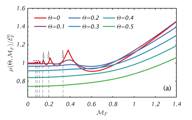
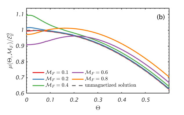
Figure 1: Relations between the chemical potential $\mu$ and (a) degeneracy $\Theta$, (b) magnetize quantum factor $\mathcal{M}_{F}$.

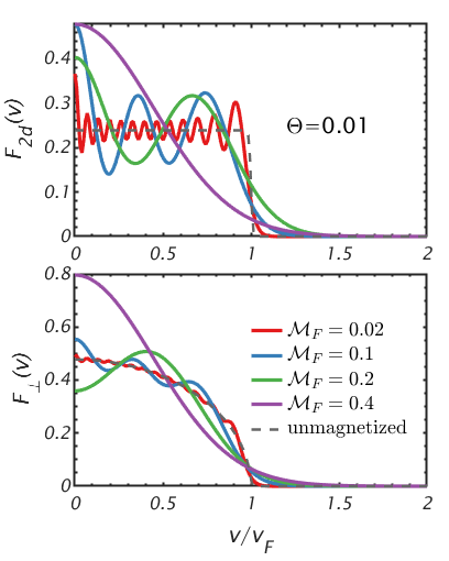
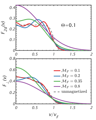
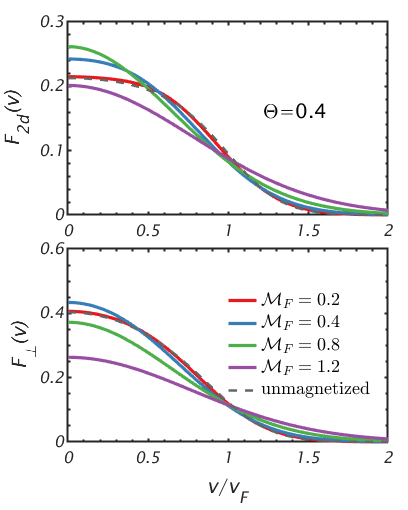
Figure 2: Equilibrium Wigner function in a magnetic field.

If the magnetic field is strong enough such that $\hbar\omega_{\mathrm{c}}$ is comparable, or even much larger than the thermal or Fermi energy. The energy of an electron is quantized into a series of Landau levels. In such case, the equilibrium Wigner function should be (see Appendix B for details)

$$f_{B}\left(\boldsymbol{v}\right) =\mathcal{A}\sum_{n=0}^{\infty}\frac{\left(-\right)^{n}{\displaystyle 2\mathrm{e}^{-\frac{mv_{\perp}^{2}}{\hbar\omega_{\mathrm{c}}}}L_{n}\left(\frac{2mv_{\perp}^{2}}{\hbar\omega_{\mathrm{c}}}\right)}}{1+{\displaystyle\mathrm{e}^{\beta\left[\frac{m}{2}v_{\parallel}^{2}+\hbar\omega_{\mathrm{c}}\left(n+\frac{1}{2}\right)-\mu\right]}}},$$ (20)

where $L_{n}\left(x\right)$ is the Laguerre function of $n$th order. The constant

$$\mathcal{A}=2\left(\frac{m}{2\pi\hbar}\right)^{3}=\frac{3n_{0}}{4\pi v_{\mathrm{F}}^{3}}$$ (21)

appears here to convert the dimensionality of the Wigner function into the density in the $x$-$v$ phase space, and the factor 2 stands for fermions. Some authors prefer to alter the velocity differential from $\mathrm{\mathrm{d}}v$ to $\mathrm{\mathrm{d}}p/\left(2\pi\hbar\right)$ to achieve this.

In high-temperature limit, i.e., $\beta\rightarrow 0$,

$$f_{B}\left(\boldsymbol{v}\right)\simeq \mathcal{A}\mathrm{e}^{-\beta\left(\frac{m}{2}v_{\parallel}^{2}-\mu+\frac{\hbar\omega_{\mathrm{c}}}{2}\right)}\mathrm{e}^{-\frac{mv_{\perp}^{2}}{\hbar\omega_{\mathrm{c}}}}\mathrm{e}^{-\beta\frac{\hbar\omega_{\mathrm{c}}}{2}}$$ (22)

$$\times\sum_{n=0}^{\infty}\left(-\mathrm{e}^{-\beta\hbar\omega_{\mathrm{c}}}\right)^{n}{\displaystyle L_{n}\left(\frac{2mv_{\perp}^{2}}{\hbar\omega_{\mathrm{c}}}\right)}$$

$$= \frac{\mathcal{A}\mathrm{e}^{\beta\mu}}{\cosh\mathcal{M}_{T}}\exp\left[-\frac{\beta m}{2}\left(v_{\parallel}^{2}+v_{\perp}^{2}\frac{\tanh\mathcal{M}_{T}}{\mathcal{M}_{T}}\right)\right],$$

where we have used the identity

$$\sum_{n=0}^{\infty}t^{n}L_{n}\left(x\right)=\frac{\mathrm{e}^{xt/\left(1-t\right)}}{1-t},$$ (23)

and

$$\mathcal{M}_{T}\equiv\frac{1}{2}\beta\hbar\omega_{\mathrm{c}}$$ (24)

is the ratio between magnetic field and temperature. Eq. (22) is identical to the zero-order Wigner-Kirkwood expansion in a strong magnetic field, firstly derived by Alastuey and Jancovici in Ref. [37]. And noting that it reduces to Maxwellian distribution when $\mathcal{M}_{T}\rightarrow 0$. By normalizing the frequency of our system to $\omega_{\mathrm{c}}$ and velocity to the Fermi velocity $v_{\mathrm{F}}$, it is found that the quantum effect is characterized by another dimensionless parameter,

$$\mathcal{M}_{F}\equiv\frac{\hbar\omega_{\mathrm{c}}}{2\mathcal{E}_{\mathrm{F}}^{0}}=\Theta\mathcal{M}_{T},$$ (25)

where $\mathcal{E}_{\mathrm{F}}^{0}=\hbar^{2}\left(3\pi^{2}n_{0}\right)^{2/3}/2m$ is the Fermi energy at zero magnetic field. Hence, $\mathcal{M}_{F}$ denotes the ratio between the lowest Landau level energy and the unmagnetized Fermi energy. As $\mathcal{M}_{F}\rightarrow 0$, the system also reduces to classical.

In low-temperature limit, i.e., $\beta\rightarrow\infty$,

$$f_{B}\left(\boldsymbol{v}\right)\simeq\mathcal{A}\sum_{n=0}^{N}\left(-\right)^{n}{\displaystyle 2\mathrm{e}^{-\frac{mv_{\perp}^{2}}{\hbar\omega_{\mathrm{c}}}}L_{n}\left(\frac{2mv_{\perp}^{2}}{\hbar\omega_{\mathrm{c}}}\right)},$$ (26)

where

$$N=\left\lfloor\frac{1}{\hbar\omega_{\mathrm{c}}}\left(\mathcal{E}_{\mathrm{F}}^{0}-\frac{1}{2}mv_{\parallel}^{2}\right)-\frac{1}{2}\right\rfloor$$ (27)

is the largest Landau quantum number that lies under the Fermi surface. From Eq. (23) we have

$$2\mathrm{e}^{-x/2}\sum_{n=0}^{\infty}\left(-1\right)^{n}L_{n}\left(x\right)=1,$$ (28)

and since now $\hbar\omega_{\mathrm{c}}\ll\mathcal{E}_{\mathrm{F}}$, namely, $N\gg 1$, one can deduce that

$$2\mathrm{e}^{-x/2}\sum_{n=0}^{N}\left(-1\right)^{n}L_{n}\left(x\right)\simeq\theta\left(x-\sqrt{2N}\right),$$ (29)

then Eq. (20) reduces to Fermi-Dirac distribution:

$$f_{0}\left(v_{\parallel},v_{\perp}\right)=\frac{\mathcal{A}}{1+\mathrm{e}^{\beta\frac{m}{2}\left(v_{\parallel}^{2}+v_{\perp}^{2}\right)-\beta\mu}}.$$ (30)

In the study of Bernstein waves, the dimension parallel to the magnetic field is usually irrelevant, which means we can integrate over $v_{\parallel}$ in advance. We define the normalized parallel and perpendicular Fermi-Dirac function here:

$$F_{\parallel}\left(v_{\parallel}\right)= n_{0}^{-1}\int_{0}^{\infty}2\pi v_{\perp}\mathrm{\mathrm{d}}v_{\perp}f_{0}\left(v_{\parallel},v_{\perp}\right)$$ (31)

$$= -\frac{3}{2m\beta v_{\mathrm{F}}^{3}}\mathrm{Li}_{1}\left[-\mathrm{e}^{\beta\left(\mu-\frac{m}{2}v_{\perp}^{2}\right)}\right]$$

$$= \frac{3}{2m\beta v_{\mathrm{F}}^{3}}\ln\left[1+\mathrm{e}^{\beta\left(\mu-\frac{m}{2}v_{\parallel}^{2}\right)}\right],$$

and

$$F_{\perp}\left(v_{\perp}\right)= n_{0}^{-1}\int_{-\infty}^{\infty}\mathrm{\mathrm{d}}v_{\parallel}f_{0}\left(v_{\parallel},v_{\perp}\right)$$ (32)

$$= -\sqrt{\frac{2\pi}{m\beta}}\mathrm{Li}_{\frac{1}{2}}\left[-\mathrm{e}^{\beta\left(\mu-\frac{m}{2}v_{\perp}^{2}\right)}\right],$$

where $\mathrm{Li}_{n}$ is the $n$-th order polylogarithm function . In the zero-temperature limit ($\beta\rightarrow\infty$), they become

$$F_{\parallel}^{0}\left(v_{\parallel}\right)=\frac{3}{4v_{\mathrm{F}}}\left(\frac{\mu}{\mathcal{E}_{\mathrm{F}}^{0}}-\frac{v_{\parallel}^{2}}{v_{\mathrm{F}}^{2}}\right),$$ (33)

and

$$F_{\perp}^{0}\left(v_{\perp}\right)=\frac{3}{\pi v_{\mathrm{F}}^{2}}\sqrt{\frac{\mu}{\mathcal{E}_{\mathrm{F}}^{0}}-\frac{v_{\perp}^{2}}{v_{\mathrm{F}}^{2}}},$$ (34)

since [38]

$$\mathrm{Li}_{s}\left(\pm\mathrm{e}^{x}\right)\overset{x\rightarrow\infty}{\sim}-\frac{x^{s}}{\Gamma\left(s+1\right)}.$$ (35)

Similarly, from Eq. (20) we have

$$F_{B\perp}\left(v_{\perp}\right)= n_{0}^{-1}\int_{-\infty}^{\infty}\frac{\mathrm{\mathrm{d}}v_{\parallel}}{2\pi\hbar/m}f_{B}\left(v_{\parallel},v_{\perp}\right)$$ (36)

$$= -\mathrm{e}^{-\frac{mv_{\perp}^{2}}{\hbar\omega_{\mathrm{c}}}}\sum_{n=0}^{\infty}\left(-\right)^{n}L_{n}\left(\frac{2mv_{\perp}^{2}}{\hbar\omega_{\mathrm{c}}}\right)$$

$$\times\sqrt{\frac{\Theta}{\pi}}\mathrm{Li}_{\frac{1}{2}}\left\{-\mathrm{e}^{\beta\left[\mu-\hbar\omega_{\mathrm{c}}\left(n+\frac{1}{2}\right)\right]}\right\},$$

and in zero-temperature limit, it is

$$F_{B\perp}^{0}\left(v_{\perp}\right)= n_{0}^{-1}\int_{-\infty}^{\infty}f_{B}\left(v_{\parallel},v_{\perp}\right)\mathrm{\mathrm{d}}v_{\parallel}$$ (37)

$$= -2\sqrt{2}\mathrm{e}^{-\frac{mv_{\perp}^{2}}{\hbar\omega_{\mathrm{c}}}}\sum_{n=0}^{\infty}\left(-\right)^{n}L_{n}\left(\frac{2mv_{\perp}^{2}}{\hbar\omega_{\mathrm{c}}}\right)$$

$$\times\sqrt{\frac{\mu}{\mathcal{E}_{\mathrm{F}}^{0}}-\mathcal{M}_{F}\left(2n+1\right)}.$$

Noticing that, if the Fermi energy (or, more generally, the chemical potential) does not vary with $\mathcal{M}_{F}$, then the lowest Landau state has an energy higher than the Fermi energy when $\mathcal{M}_{F}>1$, which is unphysical. Hence, we must assume $\mu=\mu\left(\Theta,\mathcal{M}_{F}\right)$ and $\mathcal{E}_{\mathrm{F}}=\mathcal{E}_{\mathrm{F}}\left(\mathcal{M}_{F}\right)\equiv\mu\left(0,\mathcal{M}_{F}\right)$. One can determine $\mu$ by solving the equation

$$\frac{3}{4}\mathcal{M}_{F}\sqrt{\frac{\pi}{\Theta}}\sum_{n=0}^{\infty}\mathrm{Li}_{\frac{1}{2}}\left\{-\mathrm{e}^{\left[\frac{\mu}{\mathcal{E}_{\mathrm{F}}^{0}}-\mathcal{M}_{F}\left(2n+1\right)\right]/\Theta}\right\}=1,$$ (38)

given $\Theta$ and $\mathcal{M}_{F}$, or simply

$$3\mathcal{M}_{F}\sum_{n=0}^{N}\sqrt{\frac{\mathcal{E}_{\mathrm{F}}}{\mathcal{E}_{\mathrm{F}}^{0}}-\mathcal{M}_{F}\left(2n+1\right)}=1,$$ (39)

when $\Theta\rightarrow 0$. Furthermore, when $\mathcal{M}_{F}\rightarrow 0$, the solution of Eq. (38) should be identical to the unmagnetized chemical potential $\mu\left(\Theta\right)$, namely, the solution of

$$\int_{0}^{\infty}\frac{4\pi v^{2}\mathrm{\mathrm{d}}v}{1+\mathrm{e}^{\left(v^{2}/v_{\mathrm{F}}^{2}-\mu/\mathcal{E}_{\mathrm{F}}^{0}\right)/\Theta}}=\mathcal{A}^{-1}.$$ (40)

Relations between $\mu$ and $\Theta,\mathcal{M}_{F}$ are plotted in Fig. 1. In Fig. 1 (a), one can see that the $\Theta=0$ solution exhibits multiple peaks, each corresponding to a coincidence of a Landau level and the Fermi energy, i.e., $\mathcal{E}_{\mathrm{F}}/\mathcal{E}_{\mathrm{F}}^{0}-\mathcal{M}_{F}\left(2n+1\right)$. Since $\mathcal{E}_{\mathrm{F}}/\mathcal{E}_{\mathrm{F}}^{0}\sim 1$, the peaks are located around $1/(2n+1)$, with $n\in\mathbb{Z}^{+}$. When $\mathcal{M}_{F}$ is greater than $0.38\gtrsim 1/3$, corresponding to the position of the last peak, there exists only one Landau level below the Fermi surface, which is the ground state $\hbar\omega_{\mathrm{c}}/2$. As $\mathcal{M}_{F}$ decreases, more and more Landau levels fall below the Fermi surface. This peaky behavior of Fermi energy in a magnetic field is well-known in solid-state physics area [39, 40], but is rarely discussed in plasma physics research. Also, the peaks disappear when $\Theta>0.1$ , which means that this phenomenon only occurs at extremely low temperature. In Fig. 1 (b), the chemical potential is presented as the function of $\Theta$, one can see that when $\mathcal{M}_{F}$ is small, the solution does reduce to the solution of Eq. (40) (the dashed-line).

Equilibrium Wigner functions with varies of parameters are plotted in Fig. 2, where $F_{2d}$ is the equilibrium distribution in a 2D system, namely, Eq. (20) with $v_{\parallel}=0$, and $F_{\perp}$ is defined in Eq. (36). In the $\Theta=0.01$ panel, when $\mathcal{M}_{F}<0.1$, the Wigner function is highly oscillatory around the unmagnetized Fermi-Dirac distribution curve, and when $\mathcal{M}_{F}>0.1$, the magnetized curves already differ significantly from the Fermi-Dirac curve. From the $\Theta=0.1$ and $0.4$ panel, one can see that as the temperature increases, it takes a higher $\mathcal{M}_{F}$ for the Wigner function to deviate from Fermi-Dirac shape. Moreover, when temperature is high enough, the role of $\mathcal{M}_{F}$ is to broaden the velocity distribution, just as Eq. (22) suggested.

IV Electrostatic modes in magnetized quantum plasmas

IV.1 Parallel propagation: Langmuir wave

From Eq. (11), we can see that if $k_{\perp}=0$, only $\mathcal{B}_{00}$ is non-zero, since both $J_{\ell}\left(0\right)$ and $I_{\ell}\left(0\right)$ have finite values only when $\ell=0$. Eq. (9) then reduce to the RPA eigen-equation:

$$\varepsilon\left(\omega,k_{\parallel}\right)= 1+\frac{m\omega_{\mathrm{p}}^{2}}{\hbar k_{\parallel}^{2}}\int\frac{F_{\parallel}^{+}-F_{\parallel}^{-}}{\omega-k_{\parallel}v_{\parallel}}\mathrm{\mathrm{d}}v_{\parallel}=0,$$ (41)

where $F_{\parallel}^{\pm}=F_{\parallel}\left(v_{\parallel}\pm\kappa_{\parallel}\right)$. Eq. (41) corresponds to a quantum Langmuir wave [41]. This is easy to understand since the electron wave along the magnetic field line is equivalent to a Langmuir wave in an electrostatic system. The analytic behaviors of Eq. (41) are thoroughly discussed in Ref. [42].

IV.2 Oblique Propagation

Oblique modes involve both even and odd $\ell$ modes, and finite $k_{\parallel}$ would lead to dissipative-type solutions, which makes it more complicated than the perpendicular modes. Oblique modes are left for future work.

IV.3 Perpendicular propagation: Bernstein modes

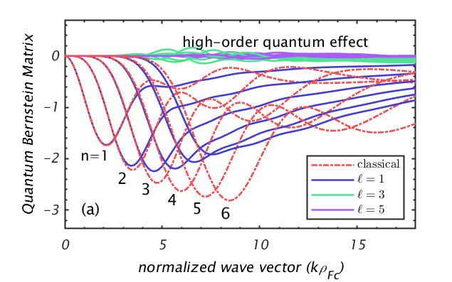
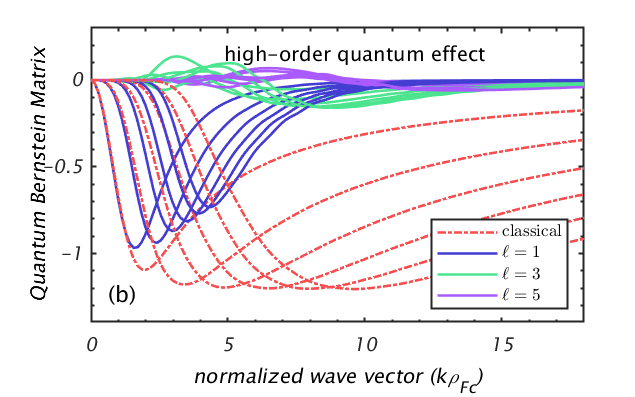
Figure 3: Zero-temperature QBM at (a) $\mathcal{M}_{F}=0.1$ and (b) $\mathcal{M}_{F}=0.8$. The curves labeled “classical” are calculated for Fermi-Dirac distribution without quantum wave effect. The subscript $n$ of some curves has been omitted for the sake of clarity.

Consider those modes propagating perpendicular to the magnetic field, i.e., $k_{\parallel}=0$. Then the quantum Harris dispersion relation reduces to

$$\varepsilon\left(\omega,k_{\perp}\right)\equiv 1+\frac{\omega_{\mathrm{p}}^{2}}{k_{\perp}^{2}}\sum_{n\in\mathbb{Z}^{+}}\frac{n\omega_{\mathrm{c}}^{2}}{\omega^{2}-n^{2}\omega_{\mathrm{c}}^{2}}\sum_{\ell\in 2\mathbb{Z}^{+}+1}\bar{\mathcal{B}}_{n\ell}\left[F_{\perp}\right],$$ (42)

which is the eigen-equation of the quantum Bernstein modes. Now the QBM becomes

$$\bar{\mathcal{B}}_{n\ell}= \frac{4m}{\hbar\omega_{\mathrm{c}}}\int 2\pi v_{\perp}\mathrm{\mathrm{d}}v_{\perp}J_{n}\left(\frac{k_{\perp}v_{\perp}}{\omega_{\mathrm{c}}}\right)$$ (43)

$$\times\left[J_{n+\ell}\left(\frac{k_{\perp}v_{\perp}}{\omega_{\mathrm{c}}}\right)+J_{n-\ell}\left(\frac{k_{\perp}v_{\perp}}{\omega_{\mathrm{c}}}\right)\right]I_{\ell}\left(\kappa_{\perp}\partial_{v_{\perp}}\right).$$

In the classical limit, we can keep only the lowest order, and further reduce $I_{1}\left(x\right)$ to $x/2$, then

$$\begin{aligned} \bar{\mathcal{B}}_{n1}=&2n\int 2\pi v_{\perp}\mathrm{\mathrm{d}}v_{\perp}J_{n}^{2}\left(\frac{k_{\perp}v_{\perp}}{\omega_{\mathrm{c}}}\right)\partial_{v_{\perp}}+\mathcal{O}\left(\hbar\right)\end{aligned}.$$ (44)

Numerical results for the components of QBM are presented in Fig. 3, where $\mathcal{M}_{F}=0.1$ for panel (a) and $\mathcal{M}_{F}=0.8$ for panel (b). The wave number is normalized to inverse of the radio between Fermi velocity and gyro-frequency, $\rho_{\mathrm{F}c}=v_{\mathrm{F}}/\omega_{\mathrm{c}}$. The red-dashed-lines, labeled “classical”, are calculated from Eq. (44) with Fermi-Dirac distribution, i.e., they only include degenerate effects, and exclude quantum wave effects. As is shown in both panel (a) and (b), the “classical” results only coincide with the $\ell=1$ quantum modes at small $k\rho_{\mathrm{F}c}$. The high-order quantum modes, which are the components in QBM with $\ell>1$, have minimal effect in the $\mathcal{M}_{F}=0.1$ case, but their impact is significant when $\mathcal{M}_{F}=0.8$. One can see that when $k\rho_{\mathrm{F}c}\gtrsim 7$, the absolute values of $\ell=3$ modes become larger than the $\ell=1$ modes.

Substitute Eq. (44) into Eq. (42), we have

$$\varepsilon\left(\omega,k_{\perp}\right)= 1+\frac{\omega_{\mathrm{p}}^{2}}{k_{\perp}^{2}}\sum_{n\in\mathbb{Z}^{+}}\frac{2n^{2}\omega_{\mathrm{c}}^{2}}{\omega^{2}-n^{2}\omega_{\mathrm{c}}^{2}}$$ (45)

$$\times\int 2\pi\mathrm{\mathrm{d}}v_{\perp}J_{n}^{2}\left(\frac{k_{\perp}v_{\perp}}{\omega_{\mathrm{c}}}\right)\partial_{v_{\perp}}F_{\text{$\perp$}}=0.$$

If the temperature is high enough such that $\Theta\gg 1$, then $F_{\perp}$ tends to Maxwellian, and Eq. (45) yields the classical Bernstein modes [1, 36]:

$$\varepsilon\left(\omega,k_{\perp}\right)=1-\frac{2\omega_{\mathrm{p}}^{2}}{\beta_{\mathrm{c}}^{2}\omega_{\mathrm{c}}^{2}}\sum_{n\in\mathbb{Z}^{+}}\frac{\exp\left(-\beta_{\mathrm{c}}^{2}\right)}{\left(\omega/n\omega_{\mathrm{c}}\right)^{2}-1}I_{n}\left(\beta_{\mathrm{c}}^{2}\right),$$ (46)

where $\beta_{\mathrm{c}}\equiv k_{\perp}v_{\mathrm{th}}/\omega_{\mathrm{c}}$.

Noticing that when the ΨDO reduces to a differential operator, the summation over $n$ can be avoided in light of the properties of Bessel functions [24, 25, 26]. It is difficult to use this scheme when a ΨDO is involved. Fortunately, the high-$n$ components have little effect on the solution and the result converges very quickly. In Ref. [26], the dispersion relations of Bernstein modes are obtained from the eigen-equation:

$$1+\frac{3\omega_{\mathrm{p}}^{2}}{\omega_{\mathrm{c}}^{2}}\int_{0}^{\pi}\mathrm{\mathrm{d}}\varphi\frac{\sin\varphi\sin\left(\varphi\Omega\right)}{\xi^{3}\sin\left(\pi\Omega\right)}\left(\sin\xi-\xi\cos\xi\right)=0,$$ (47)

where $\Omega=\omega/\omega_{\mathrm{c}}$ and $\xi=2k_{\perp}\rho_{\mathrm{F}c}\cos\left(\varphi/2\right)$. Eq. (47) is equivalent to Eq. (45) with zero-temperature Fermi-Dirac distribution Eq. (34). As mentioned in the introduction, their work neglects finite temperature and quantum wave effects. Hence, when both $\Theta$ and $\mathcal{M}_{F}$ tend to 0, our solutions should reduce to the solution of Eq. (47), which are marked by the dashed-lines in Fig. 4. Typical solutions of quantum Bernstein modes are plotted in Fig. 4. One can see that all branches of the dispersion relation shift towards smaller wave numbers due to quantum effects, with the high-$n$ branches exhibiting greater shift. And, the quantum effect is quite significant in quantum plasmas. For example, the corresponding wave number of the maximum frequency of the $n=8$ branch shrank by almost a factor of 3 from $\mathcal{M}_{F}=0$ to $1.4$.

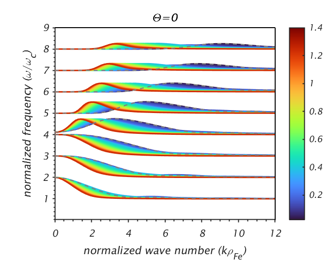
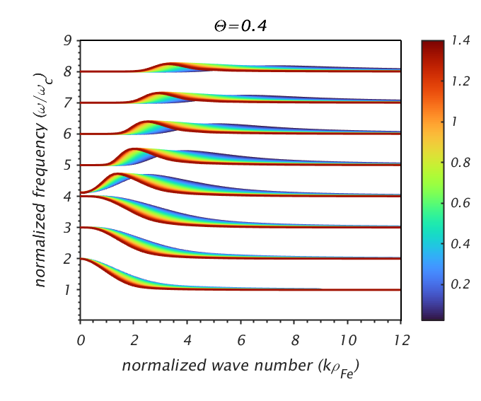
Figure 4: Quantum Bernstein modes ($\omega_{\mathrm{p}}/\omega_{\mathrm{c}}=4$) of cold ($\Theta=0$) and warm ($\Theta=0.4$) plasmas, with $\mathcal{M}_{F}=0\sim 1.4$. The dashed-lines are the solutions of Eq. (47), which is obtained by Eliasson and Shukla in Ref. [26].

V Discussion and Summary

The quantum mechanical version of the Harris dispersion relation is derived in this paper, and the non-local pseudo-differential operators arising from quantum recoil effects are addressed self-consistently. The effects of Landau quantization are also considered by introducing the magnetized Wigner equilibrium function. As a example, quantum Bernstein modes under this framework are numerically calculated.

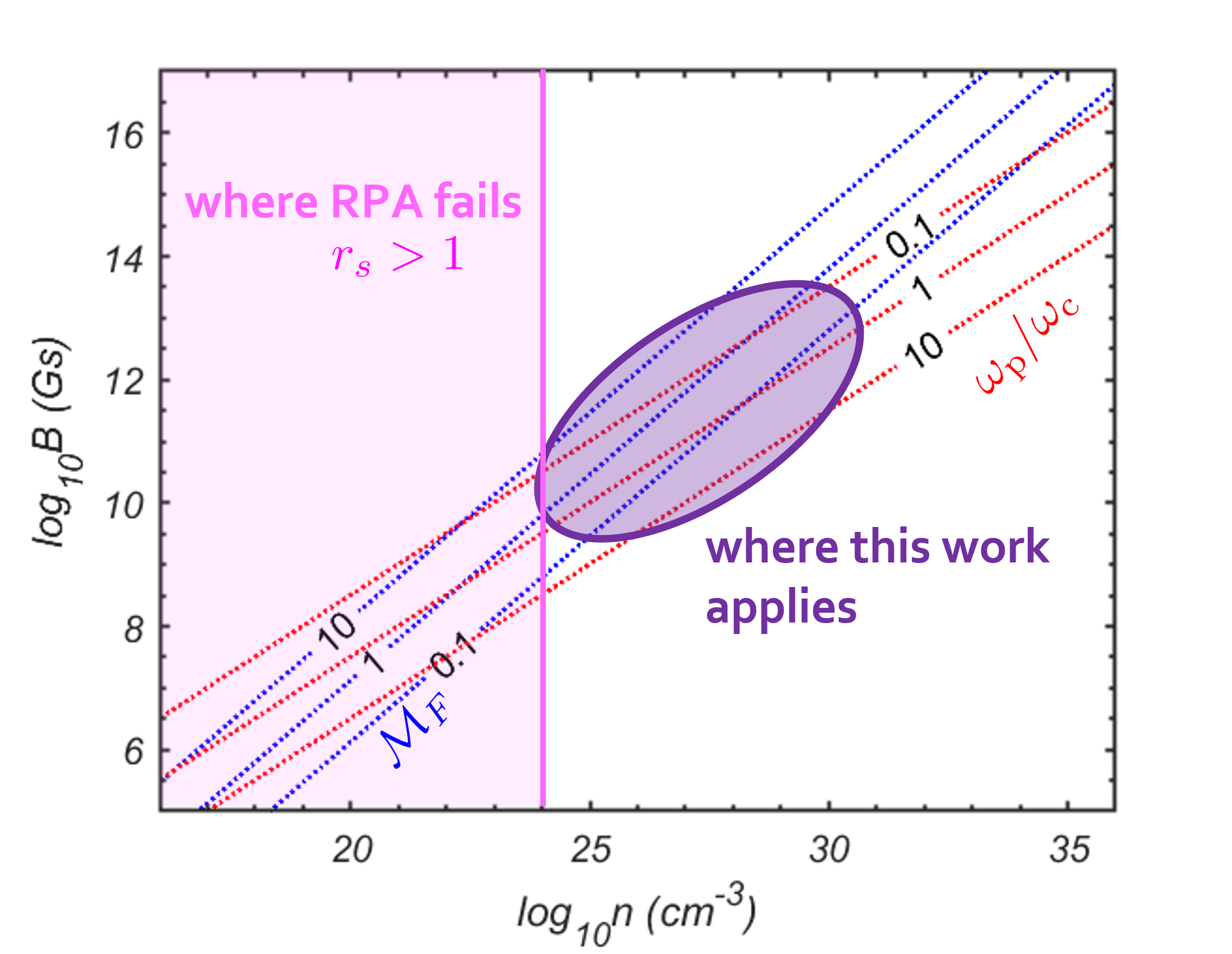
Figure 5: The applicability of this paper generally covers cases where both $\mathcal{M}_{F}$ and $\omega_{\mathrm{p}}/\omega_{\mathrm{c}}$ are of the order of 1, and RPA remains valid.

All the results obtained in the main text are in normalized units, meaning they can be applied to any density, temperature and magnetic field strength. However, a Bernstein mode is only important when $\omega_{\mathrm{p}}$ and $\omega_{\mathrm{c}}$ are of the same order. Additionally, in our paper, $\mathcal{M}_{F}$ also should be in order 1, as quantum effects can be neglected if it is too small. We marked the range of magnetic field and electron number density of this paper as a purple ellipse in Fig. 5, which is roughly where $\mathcal{M}_{F}=0.1\sim 10$ and $\omega_{\mathrm{p}}/\omega_{\mathrm{c}}=0.1\sim 10$ overlaps. Note that the ellipse does not extend into the region where $n\lesssim 10^{24}\mathrm{cm}^{-3}$, which corresponds to where the Wigner-Seitz radius $r_{s}>1$, i.e., where the RPA breaks down. Such strong magnetic field strength ($10^{9}\sim 10^{13}\mathrm{G}$) are quite common in extreme astrophysics. For example, the magnetosphere of a pulsar [43], or a high field magnetic white dwarf [44, 45]. And the electron number density range, $10^{24}\sim 10^{30}\mathrm{cm}^{-3}$, also encompasses non-relativistic white dwarfs or accretion layers of compact objects such as a black holes or a neutron stars.

Appendix A On the ΨDO $I_{\ell}\left(\kappa\partial_{v}\right)$

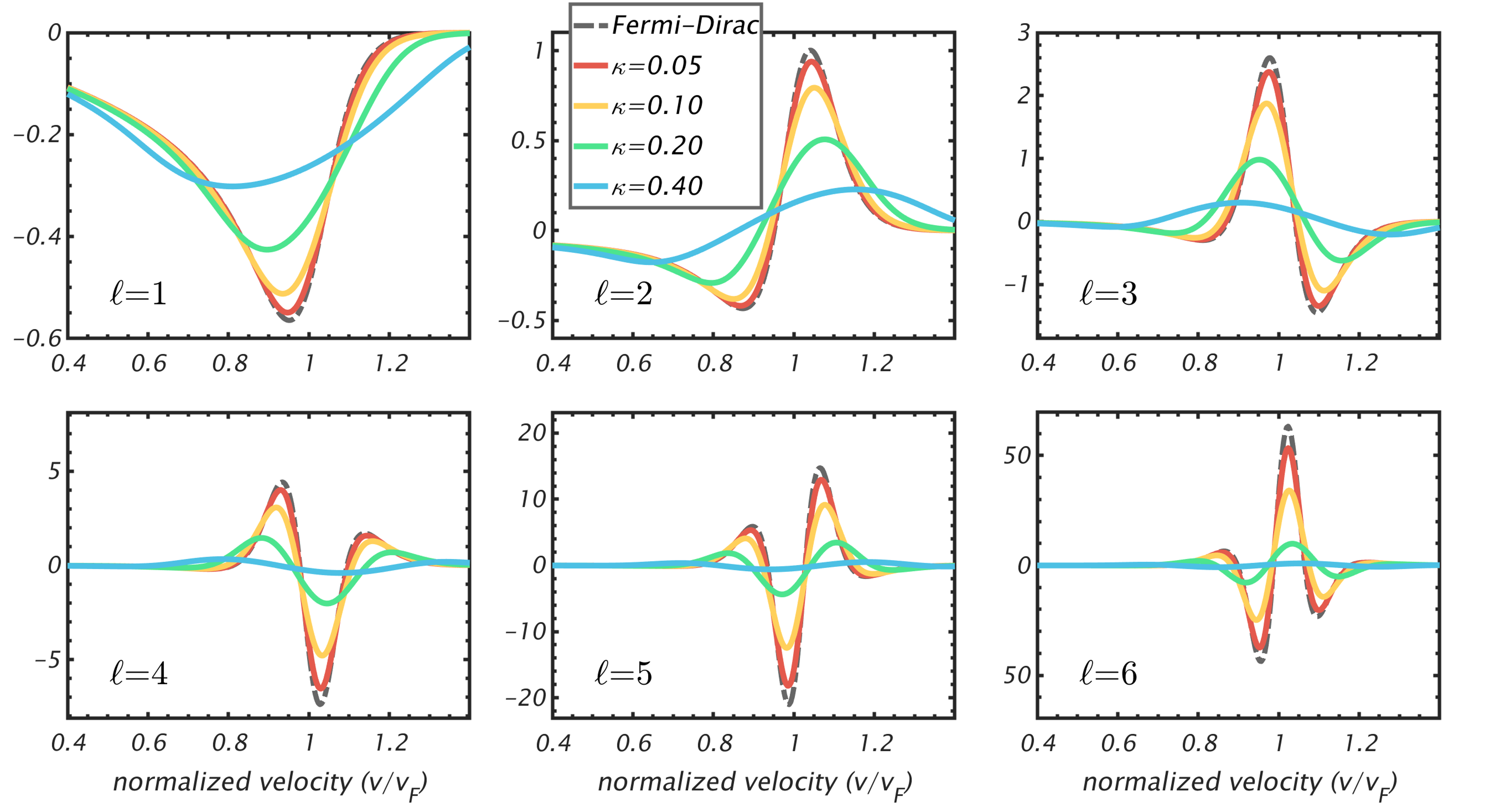
Figure 6: Numerical results of $I_{\ell}\left(\kappa\partial_{v}\right)F_{\perp}\left(v\right)/\kappa^{\ell}$ with $\ell=1\sim 6$. The black dashed-lines are the right-hand-side of Eq. (54).

To prove Eq. (19), we define $\hat{f}\left(\lambda\right)=\mathcal{F}^{-1}\left[f\left(v\right)\right]$ as the inverse Fourier coefficient of $f\left(v\right)$. Then we have:

$$I_{\ell}\left(\kappa\partial_{v}\right)f\left(v\right)= \mathrm{i}^{-\ell}\int\mathrm{\mathrm{d}}\lambda J_{\ell}\left(\kappa\lambda\right)\hat{f}\left(\lambda\right)\mathrm{e}^{-\mathrm{i}v\lambda}$$ (48)

$$= \frac{\mathrm{i}^{-\ell}}{2\pi}\iint\mathrm{\mathrm{d}}\lambda\mathrm{\mathrm{d}}v^{\prime}J_{\ell}\left(\kappa\lambda\right)f\left(v^{\prime}\right)\mathrm{e}^{-\mathrm{i}\left(v-v^{\prime}\right)\lambda}$$

$$= \mathrm{i}^{-\ell}\mathcal{F}\left[J_{\ell}\left(\kappa\lambda\right)\right]\left(v\right)*f\left(v\right),$$

where $*$ stands for convolution. And

$$\mathcal{F}\left[J_{\ell}\left(\kappa\lambda\right)\right]\left(v\right) =\frac{1}{2\pi}\int_{-\pi}^{\pi}\mathcal{F}\left[\mathrm{e}^{\mathrm{i}\kappa\lambda\sin\theta}\right]\mathrm{e}^{-\mathrm{i}\ell\theta}\mathrm{\mathrm{d}}\theta$$ (49)

$$=\mathrm{Rect}\left(\frac{v}{2\kappa}\right)\int_{-\pi}^{\pi}\delta\left(v+\kappa\sin\theta\right)\mathrm{e}^{-\mathrm{i}\ell\theta}\mathrm{\mathrm{d}}\theta,$$

where

$$\mathrm{Rect}\left(x\right)=\begin{cases}1,&\text{if }\left|x\right|<\frac{1}{2},\\ 0,&\text{otherwise},\end{cases}$$

is the unit rectangular function. Using

$$\delta\left(v+\kappa\sin\theta\right)= \frac{1}{\sqrt{\kappa^{2}-v^{2}}}\left[\delta\left(\theta+\arcsin\frac{v}{\kappa}\right)\right.$$ (50)

$$\left.+\delta\left(\theta-\arcsin\frac{v}{\kappa}+\pi\,\mathrm{sign}\frac{v}{\kappa}\right)\right],$$

then

$$\mathcal{F}\left[J_{\ell}\left(\kappa\lambda\right)\right]= \frac{\mathrm{Rect}\left(v/2\kappa\right)}{\sqrt{\kappa^{2}-v^{2}}}\left(\mathrm{e}^{\mathrm{i}\ell\arcsin\frac{v}{\kappa}}+\mathrm{e}^{\mathrm{i}\ell\pi}\mathrm{e}^{-\mathrm{i}\ell\arcsin\frac{v}{\kappa}}\right)$$ (51)

$$= \frac{2\mathrm{Rect}\left(v/2\kappa\right)}{\sqrt{\kappa^{2}-v^{2}}}\mathrm{e}^{\mathrm{i}\frac{\ell\pi}{2}}\mathbb{R}\mathrm{e}\left[\mathrm{e}^{-\mathrm{i}\frac{\ell\pi}{2}}\mathrm{e}^{\mathrm{i}\ell\arcsin\frac{v}{\kappa}}\right]$$

$$= \frac{2\mathrm{i}^{\ell}\mathrm{Rect}\left(v/2\kappa\right)}{\sqrt{\kappa^{2}-v^{2}}}\mathbb{R}\mathrm{e}\left(\frac{\kappa}{\sqrt{v^{2}-\kappa^{2}}-v}\right)^{\ell},$$

where we have used

$$\begin{aligned} \mathrm{e}^{\mathrm{i}\arcsin\frac{v}{\kappa}}&=\mathrm{i}\frac{\sqrt{v^{2}-\kappa^{2}}+v}{\kappa}=\frac{\mathrm{i}\kappa}{\sqrt{v^{2}-\kappa^{2}}-v}\end{aligned}.$$ (52)

Combining Eq. (48) and Eq. (51), we obtain Eq. (19) in the main text:

$$I_{\ell}\left(\kappa\partial_{v}\right)f\left(v\right) =\mathbb{R}\mathrm{e}\int_{-1}^{1}\frac{f\left(v-\kappa s\right)\mathrm{\mathrm{d}}s}{\pi\sqrt{1-s^{2}}\left(\sqrt{s^{2}-1}-s\right)^{\ell}}$$ (53)

$$=\frac{\left(-\right)^{\ell}}{\pi}\int_{0}^{\pi}f\left(v-\kappa\cos\varphi\right)\cos\left(\ell\varphi\right)\mathrm{\mathrm{d}}\varphi.$$

Alternatively, one can apply the sifting property of the $\delta$-function in Eq. (49) to obtain the same result.

In small $\kappa$ limit, namely, the classical limit, we have

$$\lim_{\kappa\rightarrow 0}\kappa^{-\ell}I_{\ell}\left(\kappa\partial_{v}\right)f\left(v\right)=\frac{1}{2^{\ell}\ell!}\partial_{v}^{\ell}f\left(v\right),$$ (54)

and we can make use of this feature to verify the numerical results. Take the perpendicular Fermi-Dirac distribution Eq. (32) as an example, here are its first few derivatives:

$$\partial_{v}F_{\perp} =CvP_{-\frac{1}{2}},$$ (55)

$$\partial_{v}^{2}F_{\perp} =-C\left(v^{2}P_{-\frac{3}{2}}-P_{-\frac{1}{2}}\right),$$

$$\partial_{v}^{3}F_{\perp} =-C\left(-v^{3}P_{-\frac{5}{2}}+3vP_{-\frac{3}{2}}\right),$$

$$\partial_{v}^{4}F_{\perp} =-C\left(v^{4}P_{-\frac{7}{2}}-6v^{2}P_{-\frac{5}{2}}+3P_{-\frac{3}{2}}\right),$$

$$\partial_{v}^{5}F_{\perp} =-C\left(-v^{5}P_{-\frac{9}{2}}+10v^{3}P_{-\frac{7}{2}}-15vP_{-\frac{5}{2}}\right),$$

$$\vdots$$

where

$$C=\frac{3}{4\pi v_{\mathrm{F}}^{3}},\quad P_{n}=\mathrm{Li}_{n}\left[-\mathrm{e}^{\beta\left(\mu-\frac{m}{2}v^{2}\right)}\right].$$ (56)

Numerical results of $\kappa^{-\ell}I_{\ell}\left(\kappa\partial_{v}\right)F_{\perp}\left(v\right)$ are presented in Fig. 6, with $\ell=1\sim 6$, and the dashed-lines stand for the classical operator $\partial_{v}^{\ell}F_{\perp}\left(v\right)/\left(2^{\ell}\ell!\right)$. One can see that the $\Psi$DO $I_{\ell}\left(\kappa\partial_{v}\right)$ reduces to a differential operator as $\kappa$ tends to 0, which means the non-local (quantum) ΨDO reduces to a local (classical) derivation.

Appendix B Derivation of the magnetized equilibrium Wigner function

We start from the definition of the Wigner function [46, 47]

$$f\left(\boldsymbol{x},\boldsymbol{v},t\right)=\int\frac{\mathrm{\mathrm{d}}\omega}{2\pi}g^{<}\left(\omega,\frac{m\boldsymbol{v}}{\hbar};t,\boldsymbol{x}\right)$$ (57)

where

$$g^{<}\left(\omega,\boldsymbol{q};t,\boldsymbol{x}\right)=\int\mathrm{\mathrm{d}}\tau\int\mathrm{\mathrm{d}}\boldsymbol{\xi}\mathrm{e}^{\mathrm{i}\left(\boldsymbol{\xi}\cdot\boldsymbol{q}-\omega\tau\right)}g^{<}\left(\tau,\boldsymbol{\xi};t,\boldsymbol{x}\right),$$

and $g^{<}\left(\tau,\boldsymbol{\xi};t,\boldsymbol{x}\right)$ is the less Green function $g^{<}\left(\boldsymbol{x}_{2},\boldsymbol{x}_{1};t_{2},t_{1}\right)$ in the Wigner coordinate:

$$\boldsymbol{\xi}=\boldsymbol{x}_{2}-\boldsymbol{x}_{1},\tau=t_{2}-t_{1},\boldsymbol{x}=\frac{\boldsymbol{x}_{2}+\boldsymbol{x}_{1}}{2},t=\frac{t_{2}+t_{1}}{2}.$$ (58)

In an uniform equilibrium system, $g^{<}$ is independent on $\boldsymbol{x}$ and $t$.

$$g^{<}\left(\omega,\boldsymbol{q}\right)=\bar{f}^{<}\left(\omega\right)a\left(\omega,\boldsymbol{q}\right),$$ (59)

where

$$\bar{f}^{<}\left(\omega\right)=\frac{1}{1+\mathrm{e}^{\beta\left(\hbar\omega-\mu\right)}},$$ (60)

and $a\left(\omega,\boldsymbol{q}\right)$ is the spectrum function. In the RPA limit, it is simply the Fourier component of the non-interactive single particle Green function [48, 49], which is

$$a\left(\omega,\boldsymbol{q}\right)=2\mathrm{i}\sum_{n=0}^{\infty}\frac{\left(-\right)^{n}\mathrm{e}^{-q_{\perp}^{2}\ell_{B}^{2}}L_{n}\left(2q_{\perp}^{2}\ell_{B}^{2}\right)}{\omega-\hbar q_{\parallel}^{2}/2m-\left(n+\frac{1}{2}\right)\omega_{\mathrm{c}}}.$$ (61)

Hence, by means of the residue theorem, we have

$$f\left(\frac{\hbar q_{\parallel}}{m},\frac{\hbar q_{\perp}}{m}\right)=2 \mathrm{e}^{-q_{\perp}^{2}\ell_{B}^{2}}\sum_{n=0}^{\infty}\left(-\right)^{n}L_{n}\left(2q_{\perp}^{2}\ell_{B}^{2}\right)$$ (62)

$$\times\bar{f}^{<}\left[\frac{\hbar q_{\parallel}^{2}}{2m}-\left(n+\frac{1}{2}\right)\omega_{\mathrm{c}}\right].$$

With an additional normalizing factor $\mathcal{A}$, we obtain Eq. (20) in the main text.

References

- [1] Ira B. Bernstein. Waves in a Plasma in a Magnetic Field. Phys. Rev., 109:10–21, Jan 1958.
- [2] C. Kallin and B. I. Halperin. Excitations from a filled landau level in the two-dimensional electron gas. Phys. Rev. B, 30:5655–5668, Nov 1984.
- [3] David Richards. Inelastic light scattering from inter-Landau level excitations in a two-dimensional electron gas. Phys. Rev. B, 61:7517–7525, Mar 2000.
- [4] Vidar Gudmundsson, Arne Brataas, Peter Grambow, Bernd Meurer, Thomas Kurth, and Detlef Heitmann. Bernstein modes in quantum wires and dots. Phys. Rev. B, 51:17744–17754, Jun 1995.
- [5] X.J. Zhang, Y.P. Zhao, B.N. Wan, X.Z. Gong, Y. Lin, W.Y. Zhang, Y.Z. Mao, C.M. Qin, S. Yuan, X. Deng, L. Wang, S.Q. Ju, Y. Chen, Y.D. Li, J.G. Li, J.M. Noterdaeme, and S.J. Wukitch. Experimental observation of ion heating by mode-converted ion bernstein waves in tokamak plasmas. Nuclear Fusion, 52(8):082003, aug 2012.
- [6] A. K. Ram and S. D. Schultz. Excitation, propagation, and damping of electron Bernstein waves in tokamaks. Physics of Plasmas, 7(10):4084–4094, 10 2000.
- [7] S. Shiraiwa, K. Hanada, M. Hasegawa, H. Idei, H. Kasahara, O. Mitarai, K. Nakamura, N. Nishino, H. Nozato, M. Sakamoto, K. Sasaki, K. Sato, Y. Takase, T. Yamada, and H. Zushi. Heating by an electron bernstein wave in a spherical tokamak plasma via mode conversion. Phys. Rev. Lett., 96:185003, May 2006.
- [8] B. Eliasson, M. Viktorov, D. C. Speirs, K. Ronald, D. Mansfeld, and A. D. R. Phelps. Observation of electron cyclotron harmonic emissions due to electrostatic instabilities in mirror-confined plasma. Phys. Rev. Res., 2:043272, Nov 2020.
- [9] C. Kallin and B. I. Halperin. Excitations from a filled landau level in the two-dimensional electron gas. Phys. Rev. B, 30:5655–5668, Nov 1984.
- [10] R. Roldán, M. O. Goerbig, and J.-N. Fuchs. Theory of bernstein modes in graphene. Phys. Rev. B, 83:205406, May 2011.
- [11] Dafei Jin, Ling Lu, Zhong Wang, Chen Fang, John D Joannopoulos, Marin Soljačić, Liang Fu, and Nicholas X Fang. Topological magnetoplasmon. Nature communications, 7(1):13486, 2016.
- [12] Peter H. Yoon, C. S. Wu, and Y. Li. Excitation of extraordinary bernstein waves by a beam of energetic electrons. Journal of Geophysical Research: Space Physics, 104(A9):19801–19815, 1999.
- [13] Junggi Lee, Peter H. Yoon, Jungjoon Seough, Rodrigo A. López, Junga Hwang, Jaejin Lee, and G. S. Choe. Simulation and quasi-linear theory of magnetospheric bernstein mode instability. Journal of Geophysical Research: Space Physics, 123(9):7320–7331, 2018.
- [14] W. Y. Li, D. B. Graham, Yu V. Khotyaintsev, A. Vaivads, M. André, K. Min, K. Liu, B. B. Tang, C. Wang, K. Fujimoto, C. Norgren, S. Toledo-Redondo, P. A. Lindqvist, R. E. Ergun, R. B. Torbert, A. C. Rager, J. C. Dorelli, D. J. Gershman, B. L. Giles, B. Lavraud, F. Plaschke, W. Magnes, O. Le Contel, C. T. Russell, and J. L. Burch. Electron bernstein waves driven by electron crescents near the electron diffusion region. Nature Communications, 11(1):141, 2020.
- [15] Owen Wyn Roberts, Daniel Verscharen, Yasuhito Narita, Rumi Nakamura, Zoltán Vörös, and Ferdinand Plaschke. Possible coexistence of kinetic alfvén and ion bernstein modes in sub-ion scale compressive turbulence in the solar wind. Phys. Rev. Res., 2:043253, Nov 2020.
- [16] M. Bonitz, Z. Donkó, T. Ott, H. Kählert, and P. Hartmann. Nonlinear magnetoplasmons in strongly coupled yukawa plasmas. Phys. Rev. Lett., 105:055002, Jul 2010.
- [17] T. Ott, H. Kählert, A. Reynolds, and M. Bonitz. Oscillation spectrum of a magnetized strongly coupled one-component plasma. Phys. Rev. Lett., 108:255002, Jun 2012.
- [18] Peter Hartmann, Zoltán Donkó, Torben Ott, Hanno Kählert, and Michael Bonitz. Magnetoplasmons in rotating dusty plasmas. Phys. Rev. Lett., 111:155002, Oct 2013.
- [19] S. X. Hu, B. Militzer, V. N. Goncharov, and S. Skupsky. Strong coupling and degeneracy effects in inertial confinement fusion implosions. Phys. Rev. Lett., 104:235003, Jun 2010.
- [20] Jie Zhang, WM Wang, XH Yang, D Wu, YY Ma, JL Jiao, Z Zhang, FY Wu, XH Yuan, YT Li, et al. Double-cone ignition scheme for inertial confinement fusion. Philosophical transactions of the Royal Society A, 378(2184):20200015, 2020.
- [21] Anna C Hayes, ME Gooden, E Henry, Gerard Jungman, JB Wilhelmy, RS Rundberg, C Yeamans, G Kyrala, C Cerjan, DL Danielson, et al. Plasma stopping-power measurements reveal transition from non-degenerate to degenerate plasmas. Nature Physics, 16(4):432–437, 2020.
- [22] S. J. Liu, D. Wu, T. X. Hu, T. Y. Liang, X. C. Ning, J. H. Liang, Y. C. Liu, P. Liu, X. Liu, Z. M. Sheng, Y. T. Zhao, D. H. H. Hoffmann, X. T. He, and J. Zhang. Proton-boron fusion scheme taking into account the effects of target degeneracy. Phys. Rev. Res., 6:013323, Mar 2024.
- [23] Tobias Dornheim, Sebastian Schwalbe, Panagiotis Tolias, Maximilian P. Böhme, Zhandos A. Moldabekov, and Jan Vorberger. Ab initio density response and local field factor of warm dense hydrogen. Matter and Radiation at Extremes, 9(5):057401, 07 2024.
- [24] J. A. Tataronis and F. W. Crawford. Cyclotron harmonic wave propagation and instabilities: I. Perpendicular propagation. Journal of Plasma Physics, 4(2):231–248, 1970.
- [25] J. A. Tataronis and F. W. Crawford. Cyclotron harmonic wave propagation and instabilities: II. Oblique propagation. Journal of Plasma Physics, 4(2):249–264, 1970.
- [26] Bengt Eliasson and Padma K. Shukla. Numerical and theoretical study of Bernstein modes in a magnetized quantum plasma. Physics of Plasmas, 15(10):102102, October 2008.
- [27] Z. Iqbal, G. Murtaza, K. Azra, A. Hussain, and G. Abbas. On the Bernstein mode in a degenerate anisotropic quantum plasma. Physics of Plasmas, 24(12):122114, December 2017.
- [28] N. L. Tsintsadze and L. N. Tsintsadze. Novel quantum kinetic equations of the fermi particles. Europhysics Letters, 88(3):35001, nov 2009.
- [29] Jian Zheng. Comment on “Quantum correction to Landau damping of electron plasma waves”. Physics of Plasmas, 16(5):054703, 05 2009.
- [30] F. Haas, M. Marklund, G. Brodin, and J. Zamanian. Fluid moment hierarchy equations derived from quantum kinetic theory. Physics Letters A, 374(3):481–484, January 2010.
- [31] J Zamanian, M Marklund, and G Brodin. Scalar quantum kinetic theory for spin-1/2 particles: mean field theory. New Journal of Physics, 12(4):043019, apr 2010.
- [32] Gert Brodin and Jens Zamanian. Quantum kinetic theory of plasmas. Reviews of Modern Plasma Physics, 6(1):4, 2022.
- [33] Giovanni Manfredi, Paul-Antoine Hervieux, and JérÎme Hurst. Phase-space modeling of solid-state plasmas. Reviews of Modern Plasma Physics, 3(1):13, 2019.
- [34] Anton Arnold and Herbert Steinrück. The ‘electromagnetic’ Wigner equation for an electron with spin. Zeitschrift für angewandte Mathematik und Physik ZAMP, 40:793–815, 1989. ISBN: 0044-2275 Publisher: Springer.
- [35] E. G. Harris. Unstable plasma oscillations in a magnetic field. Phys. Rev. Lett., 2:34–36, Jan 1959.
- [36] Donald A Gurnett and Amitava Bhattacharjee. Introduction to plasma physics: with space and laboratory applications. Cambridge university press, 2005.
- [37] A Alastuey and B Jancovici. Magnetic properties of a nearly classical one-component plasma in three or two dimensions: Ii. strong field. Physica A: Statistical Mechanics and its Applications, 102(2):327–343, 1980.
- [38] David Wood. The computation of polylogarithms. Technical Report 15-92*, University of Kent, Computing Laboratory, University of Kent, Canterbury, UK, June 1992.
- [39] V. P. Kurbatsky and V. V. Pogosov. Analytical model of oscillating size dependence of energy and force characteristics of subatomic metal films. Physics of the Solid State, 46(3):543–551, 2004.
- [40] Ulugbek I. Erkaboev, Ulugbek M. Negmatov, Rustamjon G. Rakhimov, Jasurbek I. Mirzaev, and Nozimjon A. Sayidov. Influence of a quantizing magnetic field on the fermi energy oscillations in two-dimensional semiconductors. International Journal of Applied Science and Engineering, 19:1–8, 2022.
- [41] Tian-Xing Hu, Jiong-Hang Liang, Zheng-Mao Sheng, and Dong Wu. Kinetic investigations of nonlinear electrostatic excitations in quantum plasmas. Physical Review E, 105(6):065203, 2022.
- [42] Tian-Xing Hu, Dong Wu, Z. M. Sheng, and J. Zhang. Exact dispersion relation of the quantum Langmuir wave. Phys. Rev. E, 109:065213, Jun 2024.
- [43] A. Philippov and M. Kramer. Pulsar Magnetospheres and Their Radiation. Annual Review of Astronomy and Astrophysics, 60(Volume 60, 2022):495–558, 2022. Publisher: Annual Reviews Type: Journal Article.
- [44] Lilia Ferrario, Domitilla de Martino, and Boris T. GÀnsicke. Magnetic white dwarfs. Space Science Reviews, 191(1):111–169, 2015.
- [45] P.-E. Tremblay, G. Fontaine, B. Freytag, O. Steiner, H.-G. Ludwig, M. Steffen, S. Wedemeyer, and P. Brassard. On the evolution of magnetic white dwarfs. The Astrophysical Journal, 812(1):19, oct 2015.
- [46] Dietrich Kremp, Manfred Schlanges, and Wolf-Dietrich Kraeft. Quantum statistics of nonideal plasmas, volume 25. Springer Science & Business Media, 2005.
- [47] Leo P Kadanoff. Quantum statistical mechanics. CRC Press, 2018.
- [48] Tsuyoshi Ueta. Green’s function of a charged particle in magnetic fields. Journal of the Physical Society of Japan, 61(12):4314–4324, 1992.
- [49] Norman J Morgenstern Horing and Musa M Yildiz. Quantum theory of longitudinal dielectric response properties of a two-dimensional plasma in a magnetic field. Annals of Physics, 97(1):216–241, 1976.