$\nu$-LPA: Fast GPU-based Label Propagation Algorithm (LPA)
for Community Detection

Abstract.

Community detection is the problem of identifying natural divisions in networks. Efficient parallel algorithms for identifying such divisions are critical in a number of applications. This report presents an optimized implementation of the Label Propagation Algorithm (LPA) for community detection, featuring an asynchronous LPA with a Pick-Less (PL) method every $4$ iterations to handle community swaps, ideal for SIMT hardware like GPUs. It also introduces a novel per-vertex hashtable with hybrid quadratic-double probing for collision resolution. On an NVIDIA A100 GPU, our implementation, $\nu$-LPA, outperforms FLPA, NetworKit LPA, and GVE-LPA by $364\times$, $62\times$, and $2.6\times$, respectively, on a server with dual 16-core Intel Xeon Gold 6226R processors — processing $3.0B$ edges/s on a $2.2B$ edge graph — and achieves $4.7\%$ higher modularity than FLPA, but $6.1\%$ and $2.2\%$ lower than NetworKit LPA and GVE-LPA.

1. Introduction

Community detection involves identifying groups of vertices within a network that have stronger connections to each other than to the rest of the network (Fortunato, 2010). When these communities are determined solely from the network’s structure, they are called intrinsic, and if each vertex belongs to only one group, the communities are considered disjoint (Gregory, 2010; Coscia et al., 2011). These groups, often referred to as clusters, provide valuable insights into the network’s structure and behavior (Fortunato, 2010; Abbe, 2018). Applications of community detection span diverse fields, including ecology (Guimerà et al., 2010), healthcare (Salathé and Jones, 2010; Bechtel et al., 2005; Haq and Wang, 2016), machine learning (Bai et al., 2024; Das and Petrov, 2011), drug discovery (Ma et al., 2019; Udrescu et al., 2020), analysis of biological networks (Kim et al., 2009; Rivera et al., 2010; Popa et al., 2011), exploration of human brain networks (He and Evans, 2010), and various other graph-related problems (Stergiou et al., 2018; Meyerhenke et al., 2017; Slota et al., 2020; Henne, 2015; Gottesbüren et al., 2021; Boldi et al., 2011; Valejo et al., 2020).

Community detection is challenging because there is no prior knowledge about the number of communities or their size distribution (Gregory, 2010). As a result, heuristic-based methods are often used to address this task (Raghavan et al., 2007; Blondel et al., 2008; Xie et al., 2011; Traag and Šubelj, 2023; Clauset et al., 2004; Duch and Arenas, 2005; Reichardt and Bornholdt, 2006; Kloster and Gleich, 2014; Traag et al., 2019; You et al., 2020; Rosvall and Bergstrom, 2008; Whang et al., 2013). The quality of detected communities is commonly evaluated using the modularity metric (Newman, 2006). Among these methods, the Label Propagation Algorithm (LPA), also known as RAK (Raghavan et al., 2007), is a popular diffusion-based heuristic that efficiently detects communities of moderate quality. LPA stands out for its simplicity, speed, and scalability compared to the Louvain method (Blondel et al., 2008), another prominent algorithm recognized for producing high-quality communities. Specifically, we observe that LPA is $2.3-14\times$ faster than Louvain, although the communities it identifies have a quality that is $3-30\%$ lower (Sahu, 2023a). Although LPA tends to produce communities with lower modularity scores, it has been shown to achieve high Normalized Mutual Information (NMI) relative to ground truth (Peng et al., 2014). In our evaluation of other label-propagation-based methods such as COPRA (Gregory, 2010), SLPA (Xie et al., 2011), and LabelRank (Xie et al., 2013), LPA emerged as the most efficient, delivering communities of comparable quality (Sahu, 2023b).

In this report, we present our parallel GPU implementation of LPA, which we call $\nu$-LPA. This implementation builds on our efficient multicore version of LPA, GVE-LPA (Sahu, 2023a). In addition to adapting the code for GPU use, we introduced several key optimizations: (1) We employ an efficient hashtable stored in global memory that uses open addressing with a hybrid approach combining quadratic probing and double hashing for collision resolution. (2) To mitigate community swaps — which can hinder algorithm convergence — we restrict each vertex to changing its label only if the new label has a smaller ID value than its current label, once every $4$ iterations. (3) We use two distinct kernels to handle low-degree and high-degree vertices: a thread-per-vertex kernel and a block-per-vertex kernel, respectively, and determine an optimal switch degree between the two. (4) Finally, unlike GVE-LPA, we use 32-bit floating-point numbers for hashtable values instead of 64-bit, which improves performance and reduces memory usage without affecting the quality of the detected communities. As no functional GPU-based implementations of LPA are publicly available, we compared our performance with state-of-the-art sequential implementations like FLPA (Traag and Šubelj, 2023), as well as multicore implementations such as NetworKit LPA (Staudt et al., 2016) and GVE-LPA (Sahu, 2023a).

2. Related work

Label Propagation Algorithm (LPA) has been widely applied in various fields. Das and Petrov (Das and Petrov, 2011) use LPA for cross-lingual knowledge transfer, employing projected labels in an unsupervised part-of-speech tagger for languages lacking labeled training data. Wang et al. (Wang et al., 2013) extend LPA to propagate labels from 2D semantic labeled datasets like ImageNet to 3D point clouds, addressing challenges in acquiring sufficient 3D labels for training classifiers. LPA has also proven effective in automatic segmentation tasks (Wang et al., 2014a). Aziz et al. (Aziz et al., 2023) apply a modified LPA for sectionalizing power systems, while Stergiou et al. (Stergiou et al., 2018) propose Shortcutting Label Propagation for distributed connected components. Boldi et al. (Boldi et al., 2011) introduce Layered Label Propagation, which uses node clusterings in various layers to reorder and compress graph nodes with the WebGraph compression framework (Boldi and Vigna, 2004). Valejo et al. (Valejo et al., 2020) present a weight-constrained variant of LPA for fast graph coarsening, allowing users to specify network size and control super-vertex weights. Mohan et al. (Mohan et al., 2017) propose a scalable method for community structure-based link prediction on large networks, combining parallel LPA for community detection with a parallel Adamic–Adar measure for link prediction. Xu et al. (Xu et al., 2019) develop a distributed temporal link prediction algorithm, DTLPLP, which updates node labels based on the weights of incident links and aggregates values from similar source nodes for link score evaluation. LPA has also been widely applied in graph partitioning (Meyerhenke et al., 2014, 2016; Zhang et al., 2020; Slota et al., 2020; Wang et al., 2014b; Akhremtsev et al., 2020; Slota et al., 2014; Meyerhenke et al., 2017; Bae et al., 2020).

Significant work has been conducted to improve the original LPA through various modifications. Farnadi et al.’s (Farnadi et al., 2015) Adaptive Label Propagation dynamically adjusts to network characteristics, like homophily or heterophily. Shen and Yang’s (SHEN and YANG, 2016) simLPA combines content-based and link-structure methods. Zarei et al.’s (Zarei et al., 2020) Weighted Label Propagation Algorithm (WLPA) for signed and unsigned networks utilizes MinHash to estimate node similarity. Sattari and Zamanifar (Sattari and Zamanifar, 2018) addressed ”monster communities” with a label-activation strategy. Zheng et al. (Zheng et al., 2018) introduced label purity, prioritized nodes with higher weighted degrees, and used an attenuation factor for faster convergence. Zhang et al.’s (Zhang et al., 2017) LPA_NI ranks nodes by importance, for label updates, while Berahmand and Bouyer’s (Berahmand and Bouyer, 2018) Label Influence Policy for Label Propagation Algorithm (LP-LPA) evaluates connection strengths and label influence — in order to enhance stability. El Kouni et al.’s (El Kouni et al., 2021) WLNI-LPA integrates node importance, attributes, and network topology to improve labeling accuracy. Roghani et al.’s (Roghani et al., 2021) Parallel Label Diffusion and Label Selection (PLDLS) identifies core nodes through triangle formation, and proceeds with standard LPA iterations. Li et al.’s (Li et al., 2015) Parallel Multi-Label Propagation Algorithm (PMLPA) uses an ankle-value based label updating strategy to detect overlapping communities. Finally, Zhang et al.’s (Zhang et al., 2023) recent method employs core nodes with degrees above the average, propagating labels layer-by-layer for detecting overlapping communities.

Some GPU-based implementations of LPA have also been proposed. Soman and Narang (Soman and Narang, 2011) presented a parallel GPU algorithm for weighted label propagation. Kozawa et al. (Kozawa et al., 2017) proposed a GPU-accelerated implementation of LPA, and discussed algorithms for handling datasets which do not fit in GPU memory. Ye et al. (Ye et al., 2023) recently developed GLP, a GPU-based framework for label propagation. In distributed environments, Maleki et al. (Maleki et al., 2020) introduced two label propagation algorithms for heterogeneous networks, while Ma et al. (Ma et al., 2018) proposed Probability and Similarity based Parallel Label Propagation Algorithm (PSPLPA), a Spark-based implementation of LPA, that uses probability and similarity.

A few open-source implementations for community detection using LPA have been developed. Fast Label Propagation Algorithm (FLPA) (Traag and Šubelj, 2023) is a fast variant of LPA that uses a queue-based approach to process only vertices with recently updated neighborhoods, without random node order shuffling. NetworKit (Staudt et al., 2016) is a software package for analyzing large graph datasets, implemented with C++ kernels and a Python frontend, and includes a parallel LPA implementation. It employs a boolean flag vector for active node tracking, uses OpenMP’s guided schedule for parallel processing, and uses std::map for storing label weights. We recently introduced GVE-LPA (Sahu, 2023a), an efficient multicore implementation of LPA that outperforms FLPA/NetworKit LPA by $139\times$/$40\times$.

Despite the utility of LPA, there is a lack of efficient and widely available GPU-based implementations, to the best of our knowledge. Our proposed $\nu$-LPA attempts to fill this gap.

3. Preliminaries

Consider an undirected graph $G(V,E,w)$, where $V$ is the set of vertices, $E$ is the set of edges, and $w_{ij}=w_{ji}$ is the weight for each edge. For an unweighted graph, each edge has a unit weight, $w_{ij}=1$. The neighbors of a vertex $i$ are denoted by $J_{i}=\{j\ |\ (i,j)\in E\}$, and the weighted degree of vertex $i$ is $K_{i}=\sum_{j\in J_{i}}w_{ij}$. The graph has $N=|V|$ vertices, $M=|E|$ edges, and the total sum of edge weights in the undirected graph is $m=\sum_{i,j\in V}w_{ij}/2$.

3.1. Community detection

Disjoint community detection aims to map each vertex $i\in V$ to a community-id $c$ from a set $\Gamma$, using a community membership function $C:V\rightarrow\Gamma$. The set of vertices in community $c$ is denoted as $V_{c}$, and the community to which vertex $i$ belongs is $C_{i}$. For a vertex $i$, its neighbors in community $c$ are represented as $J_{i\rightarrow c}=\{j\ |\ j\in J_{i}\text{ and }C_{j}=c\}$, and the sum of the corresponding edge weights is $K_{i\rightarrow c}=\sum_{j\in J_{i\rightarrow c}}w_{ij}$. The total weight of edges within a community $c$ is $\sigma_{c}=\sum_{(i,j)\in E\text{ and }C_{i}=C_{j}=c}w_{ij}$, while the total edge weight associated with $c$ is $\Sigma_{c}=\sum_{(i,j)\in E\text{ and }C_{i}=c}w_{ij}$.

3.2. Modularity

Modularity is a fitness metric for assessing the quality of communities found by heuristic-based community detection algorithms, calculated as the difference between the fraction of edges within communities and the expected fraction if edges were randomly distributed, ranging from $[-0.5,1]$, with higher values indicating better outcomes (Brandes et al., 2007). The modularity $Q$ of detected communities is determined using Equation 1, involving the Kronecker delta function ($\delta(x,y)=1$ if $x=y$, $0$ otherwise). Additionally, the delta modularity for transferring a vertex $i$ from community $d$ to $c$, represented as $\Delta Q_{i:d\rightarrow c}$, is computed using Equation LABEL:eq:delta-modularity.

(1) $$Q=\frac{1}{2m}\sum_{(i,j)\in E}\left[w_{ij}-\frac{K_{i}K_{j}}{2m}\right]\delta(C_{i},C_{j})=\sum_{c\in\Gamma}\left[\frac{\sigma_{c}}{2m}-\left(\frac{\Sigma_{c}}{2m}\right)^{2}\right]$$

(2) $$\begin{split}&\Delta Q_{i:d\rightarrow c}=\Delta Q_{i:d\rightarrow i}+\Delta Q_{i:i\rightarrow c}\\ &=\left[\frac{\sigma_{d}-2K_{i\rightarrow d}}{2m}-\left(\frac{\Sigma_{d}-K_{i}}{2m}\right)^{2}\right]+\left[0-\left(\frac{K_{i}}{2m}\right)^{2}\right]-\left[\frac{\sigma_{d}}{2m}-\left(\frac{\Sigma_{d}}{2m}\right)^{2}\right]\\ &+\left[\frac{\sigma_{c}+2K_{i\rightarrow c}}{2m}-\left(\frac{\Sigma_{c}+K_{i}}{2m}\right)^{2}\right]-\left[\frac{\sigma_{c}}{2m}-\left(\frac{\Sigma_{c}}{2m}\right)^{2}\right]-\left[0-\left(\frac{K_{i}}{2m}\right)^{2}\right]\\ &=\frac{1}{m}(K_{i\rightarrow c}-K_{i\rightarrow d})-\frac{K_{i}}{2m^{2}}(K_{i}+\Sigma_{c}-\Sigma_{d})\end{split}$$

3.3. Label Propagation Algorithm (LPA)

LPA (Raghavan et al., 2007) is a widely used diffusion-based technique for detecting communities of moderate quality in large-scale networks. It is simpler, faster, and more scalable compared to the Louvain method (Blondel et al., 2008). In LPA, each vertex $i$ initially has a unique label (community ID) $C_{i}$. During each iteration, vertices update their labels by adopting the label with the highest total interconnecting weight, as described in Equation 3. This iterative process continues until densely connected groups of vertices reach a consensus, effectively forming communities. The algorithm terminates when at least a fraction of $1-\tau$ of the vertices (with $\tau$ being the tolerance parameter) retain their current labels. LPA has a time complexity of $O(L|E|)$ and a space complexity of $O(|V|+|E|)$, where $L$ represents the number of iterations performed by the algorithm (Raghavan et al., 2007).

(3) $$C_{i}=\ \underset{c\ \in\ \Gamma}{\arg\max}{\sum_{j\in J_{i}\ |\ C_{j}=c}w_{ij}}$$

3.4. Open Addressing in Hashing

Open addressing, also known as closed hashing, is a technique for resolving collisions in hash tables. Instead of using additional data structures like linked lists (as in separate chaining), open addressing manages all entries within a single array. When a hash collision occurs, it is resolved by probing, or searching through alternative positions in the array — the probe sequence — until either the desired record is found or an empty slot is located, indicating that the key is not present in the table (Tenenbaum, 1990). Common probe sequences include: (1) Linear probing, where the step between probes is fixed (often set to $1$); (2) Quadratic probing, where the interval between probes increases according to a quadratic function; and (3) Double hashing, which uses a second hash function to determine a fixed interval for each record. These methods present trade-offs: linear probing offers the best cache performance but is highly susceptible to clustering, double hashing exhibits virtually no clustering but has weaker cache performance, and quadratic probing strikes a balance between the two. A key factor affecting the efficiency of an open addressing hash table is the load factor, which is the ratio of occupied slots to the total capacity of the array. As the load factor approaches $100\%$, the number of probes needed to find or insert a key grows significantly. For most open addressing methods, a typical load factor is around $50\%$.

3.5. Fundamentals of a GPU

The fundamental building block of NVIDIA GPUs is the Streaming Multiprocessor (SM). Each SM houses multiple CUDA cores for executing parallel threads. Additionally, SMs have shared memory, registers, and specialized function units. The number of SMs varies by GPU model, with each SM operating independently. The memory hierarchy of NVIDIA GPUs includes global, shared, and local memory. Global memory is the largest but slowest, shared memory is a low-latency memory shared among threads within an SM, while local memory serves as private storage for individual threads when register space is insufficient (Sanders and Kandrot, 2010; Nickolls and Dally, 2010).

Threads on a GPU are organized differently from those on a multicore CPU, structured into warps, thread blocks, and grids. A warp consists of 32 threads that execute instructions in lockstep. Thread blocks are groups of threads that run on the same SM. Within a thread block, warps execute together, and the SM schedules alternate warps if threads stall, such as when waiting for memory. Threads in a block can communicate using shared memory, a private, user-managed cache within each SM. A grid, which comprises multiple thread blocks, provides a higher-level structure for managing parallelism and optimizing resource usage. Thread blocks within a grid communicate exclusively through global memory, which, while slower than shared memory, allows for data exchange across different blocks (Sanders and Kandrot, 2010; Nickolls and Dally, 2010).

4. Approach

Our GPU-based implementation of LPA builds upon GVE-LPA (Sahu, 2023a), incorporating several key features: (1) An asynchronous parallel version of LPA using a single community membership vector, promoting faster convergence but potentially introducing variability in results; (2) A maximum of $20$ iterations; (3) A per-iteration tolerance of $\tau=0.05$; (4) Vertex pruning to minimize unnecessary computations, where a vertex assigns its neighbors for processing upon label change and is labeled ineligible for further processing once completed; and (5) A strict version of LPA, where each vertex selects the first label with the highest associated weight. We now discuss our GPU-specific techniques for LPA, below.

4.1. Mitigating community swaps

We first observe that the GPU implementation of LPA fails to converge for a number of input graphs, and instead continues to run for $20$ iterations. This suggests that several vertices are caught in cycles of community or label swaps. A common scenario that can lead to this issue is when two interconnected vertices continuously adopt each other’s labels. In general, this can occur when there is symmetry, i.e., when two vertices are equally connected to each other’s community. Community swaps, such as these, are more likely than may be anticipated, due to the fact the GPUs execute in lockstep. Symmetric vertices, such as the ones discussed above, can easily end up swapping labels if assigned to the same SM. Since SM assignment is typically based on vertex IDs, this problem can persist indefinitely, leading to the algorithm’s failure to converge. Hence, introducing symmetry-breaking techniques is crucial.

To address this challenge, we explore two different methods for symmetry breaking. In the Cross-Check (CC) method, after each iteration of LPA, we validate each vertex’s community change to ensure that it is a “good” change. If not, the vertex reverts to its previous community assignment. We consider a community change to be good if the new community $c^{*}$ contains a vertex $i$ with that same ID, i.e., $i=c^{*}$. In other words, a community is considered to be good if all vertices in the community have joined a certain leader vertex, and the leader vertex belongs to the same community. Note how this condition fails in the case of a community swap. Once a “bad” community change is identified, the community membership of the vertex it atomically reverted to its previous community assignment — this prevents both vertices involved in the community swap from reverting. In order to be able to perform a revert, we keep of copy of the previous label of each vertex before performing an LPA iteration. We now discuss our Pick-Less (PL) method for tackling the issue of community swaps. In this method, a vertex is only allowed to switch to a new community if the new community ID is lower than its current one. This prevents one of the pairs of vertices involved in a community swap from changing their community membership, thus breaking the symmetry. However, performing either of the two methods too frequently can hinder the algorithm’s ability to identify high-quality communities. We experiment with applying either the CC or the PL method every $1$, $2$, $3$, or $4$ iterations of LPA. We do this on large graphs from Table 1, and measure the runtimes, and modularity of obtained communities. We also explore a Hybrid (H) method, combining both the CC and PL methods in all the $16$ possible combinations.

Figures 1 and 1 show the mean relative runtime and relative modularity of obtained communities, respectively, for each of the above discussed methods. As the figures show, LPA employing the Pick-Less (PL) method performed every 4 iterations, i.e., PL4, identifies communities of the highest modularity, while being only $8\%$ slower that the fastest method (CC2). This leads us to adopt the PL4 method for our GPU implementation of LPA. Note that we employed a double-hashing based hashtable for the above experiment. A discussion on the design of hashtable is given below.

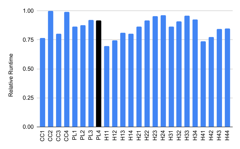
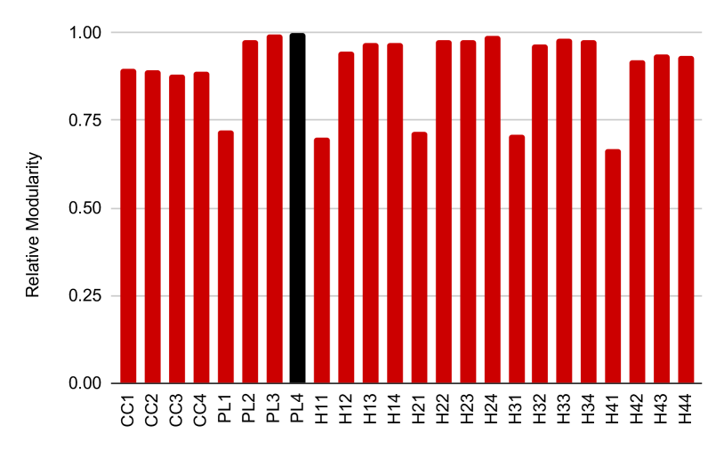
Figure 1. Relative Runtime and Modularity of obtained communities with different community swap prevention techniques — these include cross-checking and reverting bad community swaps (CC) every $1$ to $4$ iterations, enforcing picking/selection of only a label with a lower ID value (PL) every $1$ to $4$ iterations, and a hybrid of the two techniques (H) performed every $1$ to $4$ iterations.

4.2. Hashtable design

In GVE-LPA, we utilized per-thread collision-free hashtables, comprising a key list and a full-size values array (of size $|V|$) that were kept well-separated in memory. This design achieved a $15.8\times$ performance improvement compared to C++’s built-in std::unordered_ map. However, unlike multicore CPUs, GPUs operate with a far greater number of threads, making it impractical to allocate $O(|V|)$ memory for each thread on a GPU. This challenge is compounded by the fact that GPUs have limited memory capacity.

To address these challenges, we instead opt for a hashtable based on open-addressing. This hashtable $H$ is composed of two arrays: a keys array $H_{k}$ and a values array $H_{v}$ — $H_{k}$ stores neighboring labels of the current vertex, while $H_{v}$ holds the corresponding edge weights. The size of the hashtable must be at least as large as the degree of the vertex being processed. However, since a vertex can have a degree as high as $|V|$, allocating a fixed memory block for the hashtable per thread would be impractical, and put us back at square one. Instead, we create a dedicated hashtable for each vertex in the graph. Given that the total number of edges in the graph is $|E|$, the cumulative size of all hashtables can be bounded by $O(|E|)$. In order to ensure a load factor below $100\%$, we allocate twice the degree of each vertex as the size of its corresponding hashtable. This means that memory allocation for all per-vertex hashtables only requires two calls of size $2|E|$: one for all $H_{k}$s, and another for the $H_{v}$s. Each thread can then retrieve the hashtable $H$ associated with a vertex, $i$, by computing offsets. This is done using the same offset information provided in the Compressed Sparse Row (CSR) format: specifically, the starting position of the vertex’s edges and its degree. For efficient hash computation, we set the size of each hashtable to $nextPow2(D_{i})-1$, where $D_{i}$ is the vertex’s degree. This enables the use of the $\bmod$ operator as a simple hash function to find the slot index for a given key. Figure 2 provides a visual representation of this per-vertex hashtable design. The hashtable supports a few key operations: accumulating weights for matching keys, clearing the hashtable, and identifying the key with the highest associated weight. Deletion of keys is not required for our scenario. To ensure thread safety when accessing and updating the hashtable, we utilize atomic operations. For example, when accumulating weights, we use atomic addition to update $H_{k}$ and $H_{v}$. This prevents race conditions when multiple threads attempt to modify the same key’s weight simultaneously.

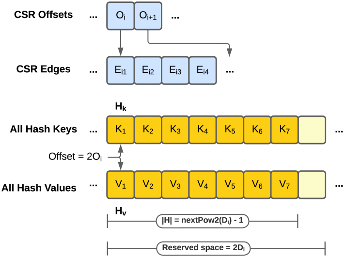
Figure 2. Illustration of per-vertex open-addressing hashtables for our GPU implementation of LPA. Each vertex $i$ has a hashtable $H$ with a keys array $H_{k}$ and a values array $H_{v}$. Memory for all vertices’ hash key and value arrays is allocated together. The hashtable’s offset for vertex $i$ is $2O_{i}$, where $O_{i}$ is its CSR offset. The memory reserved for the hashtable is $2D_{i}$, with $D_{i}$ being the vertex’s degree. The hashtable’s capacity, or maximum key-value pairs, is $nextPow2(D_{i})-1$.

We now examine three common techniques for resolving collisions in hashing: linear probing, quadratic probing, and double hashing. As previously mentioned, linear probing is cache-efficient but tends to experience high clustering, increasing the likelihood of repeated collisions. In contrast, double hashing significantly reduces clustering but lacks cache efficiency. Quadratic probing falls somewhere between the two in terms of clustering and cache efficiency. It is important to note that repeated collisions can lead to thread divergence, which can severely impact algorithm performance. In our implementation, we set the probe step for linear probing to $1$. For quadratic probing, we begin with an initial probe step of $1$ and double it with each subsequent collision. For double hashing, we use a secondary prime, $p_{2}=nextPow2(p_{1})-1$, which is co-prime with $p_{1}=|H|$. This secondary prime, $p_{2}$, is utilized with the modulo operator to calculate the probe step for each key. To further reduce collisions, we consider a hybrid collision resolution technique, which we refer to as quadratic-double. In this method, the probe step is the sum of the steps calculated by quadratic probing and double hashing. Figure 3 compares the mean relative runtime of our GPU implementation of LPA using these four collision resolution strategies, with the per-vertex hashtables, on the large graphs presented in Table 1.

As Figure 3 shows, the quadratic-double approach delivers the best performance. Specifically, it is $2.8\times$, $3.7\times$, and $3.2\times$ times faster than LPA implementations that use linear probing, quadratic probing, and double hashing, respectively. This suggests that the hybrid approach effectively balances clustering and cache efficiency. Consequently, we adopt the quadratic-double strategy for our GPU-based LPA implementation. We also tested a coalesced chaining-based hashtable — a collision resolution technique that combines aspects of separate chaining and open addressing — utilizing another nexts array $H_{n}$. However, it did not improve performance. We also experimented with shared memory-based hashtables for low-degree vertices, but saw little to no performance gain.

Figure 3. Relative Runtime with using Linear probing, Quadriatic probing, Double hashing, and a hybrid of Quadriatic probing and Double hashing (Quadriatic-double) for collision resolution in the per-vertex hashtables.

4.3. Partitioning work between two kernels

Processing each vertex in the graph with a thread-block per vertex may not be efficient, especially for low-degree vertices. If a vertex has a degree lower than $32$ — the warp size on NVIDIA GPUs — many threads in the warp would remain idle. Since graphs often contain a large number of such low-degree vertices, we opt to handle them using a thread-per-vertex approach (Wu et al., 2010).

To implement this, we divide the vertices into two partitions: low-degree and high-degree. Low-degree vertices are processed using a thread-per-vertex kernel, while high-degree vertices are handled with a block-per-vertex kernel. We experiment with different partition thresholds, ranging from a degree of $2$ to $256$, using graphs from our dataset. As shown in Figure 4, a switch degree of $32$ yields the best performance (highlighted in the figure). Note that in the thread-per-vertex kernel, only a single thread operates on the hashtable. This eliminates the need for atomic operations.

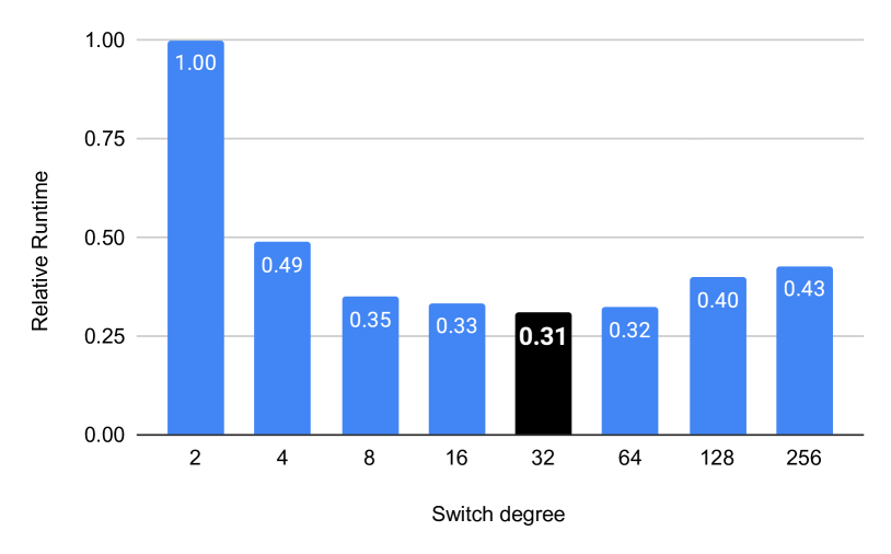
Figure 4. Relative Runtime with various switch degrees, i.e., switching point by vertex degree between the thread-per-vertex kernel vs. block-per-vertex kernel, ranging from $2$ to $256$. Vertices with degree lower than the switch degree are processed by the thread-per-vertex kernel, while the remaining vertices are processed by the block-per-vertex kernel (the vertices are partitioned accordingly).

4.4. Selecting datatype for hashtable values

Finally, we experiment with using 32-bit floating-point numbers as hashtable values, i.e., for aggregated label weights, instead of 64-bit floating-point numbers. Figure 5 illustrates the relative runtime comparison between the two. Our findings indicate that using 32-bit floats does not compromise the quality of the communities obtained, while providing a moderate speedup. As a result, we adopt 32-bit floats as hashtable values in our GPU implementation of LPA.

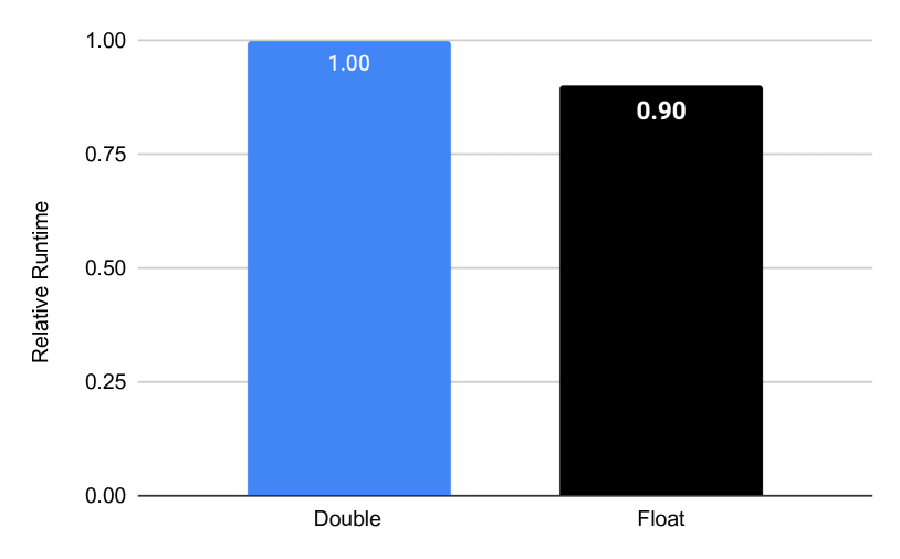
Figure 5. Relative Runtime with using 32-bit floating point values (Float) compared to 64-bit floating point values (Double) for the aggregated weights (values) in the hashtable.

4.5. Our optimized LPA implementation

We now explain our GPU implementation of LPA, which we refer to as $\nu$-LPA, in Algorithms 1 and 2. In $\nu$-LPA, the symbol $\nu$ is a reference to “video card”. $\nu$-LPA has a time complexity of $O(KM)$, where $K$ is the number of iterations performed, and a space complexity of $O(M)$. In contrast, GVE-LPA has a space complexity of $O(TN+M)$, where $T$ represents the number of threads being used.

4.5.1. Main step of $\nu$-LPA

The main step of $\nu$-LPA is described in Algorithm 1. Here, the function lpa() takes the input graph $G$ and outputs the community membership (or label) for each vertex. In lines 13 to 14, we start by assigning a unique community label to each vertex — effectively making each vertex its own community — and mark all vertices as unprocessed. Next, multiple iterations of label propagation are carried out (lines 15 to 20). As discussed earlier, we use the Pick-Less (PL) method every $\rho=4$ iterations, where a vertex can only switch to a new community if the new community ID is smaller than its current one (lines 17 to 18) — this helps mitigate community swaps. During each iteration, unprocessed vertices choose the label with the highest interconnecting weight via the lpaMove() function (line 19). In line 20, we verify whether the fraction of changed vertices, $\Delta N/N$, is below the tolerance threshold $\tau$ and PL is disabled. If it is, the labels have converged, and the algorithm terminates, returning the identified communities in line 21.

Each iteration of $\nu$-LPA is performed in the lpaMove() function. Here, we first initialize the total count of changed vertices, $\Delta N$, the number of changed vertices per thread or thread-block $\Delta N_{T}$, and allocate space for the buffers $buf_{k}$ and $buf_{v}$ (each of size $2|E|$) for the per-vertex hash key arrays $H_{k}$ and hash value arrays $H_{v}$ (lines 24-26). Next, we perform the parallel update of labels for each vertex $i$ in the graph (lines 27-47). First, we mark vertex $i$ as processed. Then, if the degree of $i$ is less than SWITCH_DEGREE (set to 32), it is processed by an individual thread. Otherwise, a thread-block is used. For each vertex $i$, we calculate the size $|H|=p_{1}$ of the hashtable for $i$, and select a secondary prime number for quadratic-double hashing. The hashtable’s memory, $H_{k}$ and $H_{v}$, is identified from the buffers $buf_{k}$ and $buf_{v}$ (lines 31-35). In line 37, we first clear the hashtable in parallel, preparing for the identification of the most weighted label for $i$. Subsequently, we iterate over each neighbor $j$ of vertex $i$, accumulating its weighted label $(C[j],w)$ into the hashtable $H$ (lines 38-40). Afterward, we determine the most weighted label $c^{*}$ for vertex $i$ by performing a parallel max-reduce operation on the hashtable (line 41). If the PL method is disabled or $c^{*}$ is smaller than $i$’s previous label, vertex $i$ adopts the new label $c^{*}$, the count of changed vertices per thread is updated, and the neighbors of vertex $i$ are marked as unprocessed in parallel (lines 43-47). Once all vertices assigned to the current thread/thread-block are processed, the global count of changed vertices $\Delta N$ is updated using atomic operations (line 48), and returned (line 49). Note that the community labels for vertices are updated in-place.

Algorithm 1 $\nu$-LPA: Our GPU-based LPA.

1:$G(V,E)$: Input graph

2:$C$: Community membership of each vertex

3:$\Delta N$: Number of changed vertices, overall

4:$\Delta N_{T}$: Changed vertices per thread / thread-block

5:$c^{*}$: Most weighted label for vertex $i$

6:$H$: Per thread / thread-block hashtable

7:$p_{1}$: Capacity of $H$, and also a prime

8:$p_{2}$: Secondary prime, such that $p_{2}>p_{1}$

9:$l_{i}$: Number of iterations performed

10:$\tau$: Per iteration tolerance

11:

12:function lpa($G$)

13:     Vertex membership: $C\leftarrow[0..|V|)$

14:     Mark all vertices in $G$ as unprocessed

15:     for all $l_{i}\in[0\ \dots\ \text{\small{MAX\_ITERATIONS}})$ do

16:         $\rhd$ Mitigate community swaps with pick-less mode

17:         if $l_{i}\bmod\rho=0$ then Enable pick-less mode

18:         else Disable pick-less mode          

19:         $\Delta N\leftarrow lpaMove(G,C)$

20:         if not pick-less and $\Delta N/N<\tau$ then break               

21:     return $C$

22:

23:function lpaMove($G,C$)

24:     $\Delta N\leftarrow 0$ ; $\Delta N_{T}\leftarrow\{\}$

25:     $buf_{k}\leftarrow\{\}$ ; $buf_{v}\leftarrow\{\}$

26:     $\Delta N_{T}[t]\leftarrow 0$ on each thread / thread-block

27:     for all unprocessed $i\in V$ in parallel do

28:         $\rhd$ Mark vertex $i$ as processed

29:         $\rhd$ If degree of $i<$ SWITCH_DEGREE,

30:         $\rhd$ process using a thread, else use a thread-block

31:         $p_{1}\leftarrow nextPow2(G.degree(i))-1$

32:         $p_{2}\leftarrow nextPow2(p_{1})-1$

33:         $\theta_{H}\leftarrow 2*G.offset(i)$

34:         $H_{k}\leftarrow buf_{k}[\theta_{H}:\theta_{H}+p_{1}]$ $\triangleright$ $H$ is shared, if using

35:         $H_{v}\leftarrow buf_{v}[\theta_{H}:\theta_{H}+p_{1}]$ $\triangleright$ a thread-block

36:         $\rhd$ Identify most weighted label for vertex $i$

37:         $hashtableClear(H)$ in parallel

38:         for all $(j,w)\in G.neighbors(i)$ in parallel do

39:             if $j=i$ then continue              

40:             $hashtableAccumulate(H,p_{1},p_{2},C[j],w)$          

41:         $c^{*}\leftarrow hashtableMaxKey(H)$ in parallel

42:         $\rhd$ Change label of vertex $i$ to most weighted label $c^{*}$

43:         if $c^{*}\neq C[i]$ and $($not pick-less or $c^{*}\leq C[i])$ then

44:             $C[i]\leftarrow c^{*}$

45:             $\Delta N_{T}[t]\leftarrow\Delta N_{T}[t]+1$

46:             for all $j\in G.neighbors(i)$ in parallel do

47:                  Mark $j$ as unprocessed                             

48:     $atomicAdd(\Delta N,\Delta N_{T}[t])$ on each thread / thread-block

49:     return $\Delta N$

4.5.2. Hashtable for $\nu$-LPA

We now turn our attention to Algorithm 2, which is designed to accumulate the associated weights of labels for a vertex within its hashtable, while efficiently handling potential collisions through a hybrid quadratic-double probing strategy. Given a key $k$ and its corresponding value $v$, the algorithm aims to locate an appropriate slot in the hashtable $H$ (with $p_{1}$ slots) where the key can either be inserted or its value updated. The process begins by calculating an initial slot index $s$ using the primary hash function: $s=i\bmod p_{1}$ (line 10), where $i$ starts as the key $k$ and is adjusted incrementally using a step size $\delta i$. If the computed slot $s$ is empty (denoted by $\phi$) or already contains the key $k$, the algorithm proceeds to update or insert the value in $H_{v}[s]$.

The approach differs depending on whether the hashtable is accessed by multiple threads (shared scenario, lines 12-15) or a single thread (non-shared scenario, lines 17-21). In the non-shared case, the algorithm directly modifies $H_{k}$ and $H_{v}$. In the shared case, atomic operations ensure thread safety: an atomicCAS() operation attempts to atomically set $H_{k}[s]$ to $k$ if the slot is empty. If this operation succeeds, or if the slot already contains $k$, the atomicAdd() operation updates $H_{v}[s]$ by adding the new value $v$. If the slot is occupied by a different key, hybrid quadratic-double probing is triggered as follows: $\delta i$ is doubled and adjusted using $k\bmod p_{2}$ (line 23), where $p_{2}$ is a secondary prime larger than $p_{1}$. This process repeats iteratively (lines 9-23) for up to MAX_RETRIES attempts. If a suitable slot is not located within the maximum retries, the function returns a failed status — though this scenario is avoided by ensuring the hashtable has sufficient capacity for all entries.

Algorithm 2 Accumulating associated weights of labels.

1:$H$: Hashtable with $p_{1}$ slots ($H_{k}$: keys, $H_{v}$: values)

2:$p_{1}$: Capacity of $H$, and also a prime

3:$p_{2}$: Secondary prime, such that $p_{2}>p_{1}$

4:$k,v$: Key, associated value to accumulate

5:$s$: Slot index

6:

7:function hashtableAccumulate($H,p_{1},p_{2},k,v$)

8:     $i\leftarrow k$ ; $\delta i\leftarrow 1$

9:     for all $t\in[0\ \dots\ \text{\small{MAX\_RETRIES}})$ do

10:         $s\leftarrow i\bmod p_{1}$ $\triangleright$ $1^{st}$ hash function

11:         if is not shared then

12:              if $H_{k}[s]=k$ or $H_{k}[s]=\phi$ then

13:                  if $H_{k}[s]=\phi$ then $H_{k}[s]\leftarrow k$                   

14:                  $H_{v}[s]\leftarrow v$

15:                  return $done$               

16:         else

17:              if $H_{k}[s]=k$ or $H_{k}[s]=\phi$ then

18:                  $k_{old}\leftarrow atomicCAS(H_{k}[s],\phi,k)$

19:                  if $k_{old}=\phi$ or $k_{old}=k$ then

20:                       $atomicAdd(H_{v}[s],v)$

21:                       return $done$                                           

22:         $i\leftarrow i+\delta i$

23:         $\delta i\leftarrow 2*\delta i+(k\bmod p_{2})$ $\triangleright$ $2^{nd}$ hash function      

24:     return $failed$

5. Evaluation

5.1. Experimental Setup

5.1.1. System used

We utilize a server featuring an NVIDIA A100 GPU, which has 108 Streaming Multiprocessors (SMs), each with 64 CUDA cores. The GPU has $80$ GB of global memory, a bandwidth of $1935$ GB/s, and $164$ KB of shared memory per SM. The server is powered by an AMD EPYC-7742 processor with 64 cores running at $2.25$ GHz, has $512$ GB of DDR4 RAM, and runs Ubuntu 20.04. For evaluating CPU-only implementations of LPA, we use a separate server which has two Intel Xeon Gold 6226R processors, with each processor having 16 cores clocked at $2.90$ GHz. Each core of the CPU is equipped with a $1$ MB L1 cache, a $16$ MB L2 cache, and a $22$ MB shared L3 cache. The system is configured with $512$ GB of RAM and runs on CentOS Stream 8.

5.1.2. Configuration

We utilize 32-bit integers for vertex identifiers and 32-bit floating-point numbers for edge weights and hash table values. For compilation, we employ GCC 9.4, OpenMP 5.0, and CUDA 11.4 on the GPU system. On the CPU-only system, we rely on GCC 8.5 and OpenMP 4.5.

5.1.3. Dataset

The graphs used in our experiments are listed in Table 1, and they are sourced from the SuiteSparse Matrix Collection (Kolodziej et al., 2019). The graphs vary in size, with the number of vertices ranging from $3.07$ million to $214$ million, and the number of edges ranging from $25.4$ million to $3.80$ billion. We ensure that the edges are undirected and weighted, with a default weight of $1$.

Table 1. List of $13$ graphs obtained SuiteSparse Matrix Collection (Kolodziej et al., 2019) (directed graphs are marked with $*$). Here, $|V|$ is the number of vertices, $|E|$ is the number of edges (after adding reverse edges), and $D_{avg}$ is the average degree, and $|\Gamma|$ is the number of communities obtained with $\nu$-LPA.

Graph	$|V|$	$|E|$	$D_{avg}$	$|\Gamma|$
Web Graphs (LAW)
indochina-2004∗	7.41M	341M	41.0	215K
uk-2002∗	18.5M	567M	16.1	541K
arabic-2005∗	22.7M	1.21B	28.2	364K
uk-2005∗	39.5M	1.73B	23.7	1.14M
webbase-2001∗	118M	1.89B	8.6	8.51M
it-2004∗	41.3M	2.19B	27.9	901K
sk-2005∗	50.6M	3.80B	38.5	?
Social Networks (SNAP)
com-LiveJournal	4.00M	69.4M	17.4	145K
com-Orkut	3.07M	234M	76.2	2.21K
Road Networks (DIMACS10)
asia_osm	12.0M	25.4M	2.1	2.01M
europe_osm	50.9M	108M	2.1	7.51M
Protein k-mer Graphs (GenBank)
kmer_A2a	171M	361M	2.1	28.8M
kmer_V1r	214M	465M	2.2	34.7M

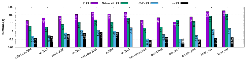
(a) Runtime in seconds (logarithmic scale) with FLPA, NetworKit LPA, GVE-LPA, and $\nu$-LPA

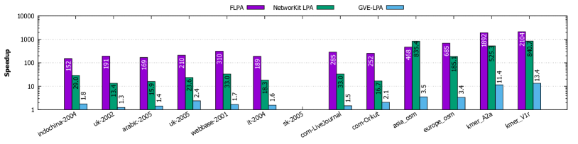
(b) Speedup of $\nu$-LPA (logarithmic scale) with respect to FLPA, NetworKit LPA, and GVE-LPA.

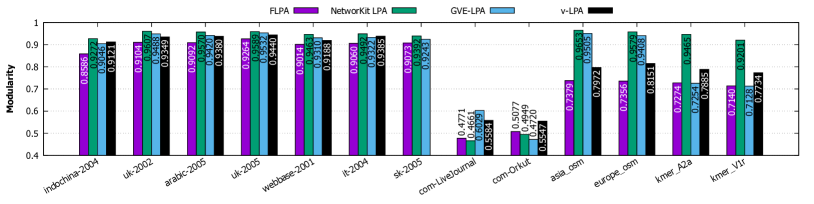
(c) Modularity of communities obtained with FLPA, NetworKit LPA, GVE-LPA, and $\nu$-LPA.

Figure 6. Runtime in seconds (log-scale), speedup (log-scale), and modularity of obtained communities (log-scale) with FLPA, NetworKit LPA, GVE-LPA, and $\nu$-LPA for each graph in the dataset.

5.2. Performance Comparison

We now evaluate the performance of $\nu$-LPA in comparison with FLPA (Traag and Šubelj, 2023), NetworKit LPA (Staudt et al., 2016), and GVE-LPA (Sahu, 2023a). FLPA is a sequential implementation, whereas both NetworKit LPA and GVE-LPA are parallel multicore implementations. For FLPA, we check out the appropriate branch containing the modified igraph_community _label_propagation() function, update the label propagation example in C to load the input graph from a file, and measure the runtime of igraph_community_label_propagation() using the IGRAPH_LPA_FAST variant and gettimeofday(). For NetworKit, we utilize a Python script to execute PLP (Parallel Label Propagation) and measure the total runtime with getTiming(). For GVE-LPA, we run the provided script. We repeat the runtime measurement five times per graph to obtain an average, and record the modularity of communities identified by each implementation.

Figure 6(a) presents the runtimes of FLPA, NetworKit LPA, GVE-LPA, and $\nu$-LPA for each graph in the dataset, while Figure 6(b) illustrates the speedup of $\nu$-LPA relative to the other implementations. Note that $\nu$-LPA fails to run on the sk-2005 graph due to out-of-memory issue, and therefore, its results for this graph are not shown. $\nu$-LPA demonstrates an average speedup of $364\times$, $62\times$, and $2.6\times$ compared to FLPA, NetworKit LPA, and GVE-LPA, respectively. We also attempted to assess the performance of the GPU implementation of LPA by Kozawa et al. (Kozawa et al., 2017), but it failed to run, crashing during graph loading. On the it-2004 graph, $\nu$-LPA identifies communities in just $1.6$ seconds, achieving a processing rate of $3.0$ billion edges per second. Figure 6(c) shows the modularity of the communities identified by each method. On average, $\nu$-LPA achieves $4.7\%$ higher modularity than FLPA (notably on road networks and protein k-mer graphs), but $6.1\%$ lower modularity than NetworKit LPA (especially on on the same set of graphs), and $2.2\%$ lower modularity than GVE-LPA (particularly on road networks). We plan to address this discrepancy in future work. Nonetheless, the current results suggest that $\nu$-LPA is a strong candidate for web graphs and social networks. For road networks, however, GVE-LPA appears to be the most effective, while NetworKit LPA is recommended for protein k-mer graphs.

6. Conclusion

In conclusion, in this technical report, we introduced an efficient implementation of the Label Propagation Algorithm (LPA) for community detection. It used an asynchronous implementation of LPA, which employed a Pick-Less (PL) approach every $4$ iterations for handling community swaps — a scenario more likely to occur on SIMT hardware, such as GPUs. Additionally, it utilized a novel open-addressing-based per-vertex hashtable with hybrid quadratic-double probing for collision resolution. On a server with an NVIDIA A100 GPU, our GPU implementation of LPA, referred to as $\nu$-LPA, outperformed FLPA, NetworKit LPA, and GVE-LPA by $364\times$, $62\times$, and $2.6\times$, respectively, running on a server equipped with dual 16-core Intel Xeon Gold 6226R processors — achieving a processing rate of $3.0B$ edges/s on a $2.2B$ edge graph — while identifying communities with $4.7\%$ higher modularity than FLPA, but $6.1\%$ and $2.2\%$ lower modularity than NetworKit LPA and GVE-LPA.

- (1)
- Abbe (2018) Emmanuel Abbe. 2018. Community detection and stochastic block models: recent developments. Journal of Machine Learning Research 18, 177 (2018), 1–86.
- Akhremtsev et al. (2020) Yaroslav Akhremtsev, Peter Sanders, and Christian Schulz. 2020. High-quality shared-memory graph partitioning. IEEE Transactions on Parallel and Distributed Systems 31, 11 (2020), 2710–2722.
- Aziz et al. (2023) Tarique Aziz, Muhammad Waseem, Shengyuan Liu, Zhenzhi Lin, Yuxuan Zhao, and Kaiyuan Pang. 2023. A novel power system sectionalizing strategy based on modified label propagation algorithm. In 2023 6th International Conference on Energy, Electrical and Power Engineering (CEEPE). IEEE, 807–812.
- Bae et al. (2020) Minho Bae, Minjoong Jeong, and Sangyoon Oh. 2020. Label propagation-based parallel graph partitioning for large-scale graph data. IEEE Access 8 (2020), 72801–72813.
- Bai et al. (2024) Yuhe Bai, Camelia Constantin, and Hubert Naacke. 2024. Leiden-Fusion Partitioning Method for Effective Distributed Training of Graph Embeddings. In Joint European Conference on Machine Learning and Knowledge Discovery in Databases. Springer, 366–382.
- Bechtel et al. (2005) Joel J Bechtel, William A Kelley, Teresa A Coons, M Gerry Klein, Daniel D Slagel, and Thomas L Petty. 2005. Lung cancer detection in patients with airflow obstruction identified in a primary care outpatient practice. Chest 127, 4 (2005), 1140–1145.
- Berahmand and Bouyer (2018) Kamal Berahmand and Asgarali Bouyer. 2018. LP-LPA: A link influence-based label propagation algorithm for discovering community structures in networks. International Journal of Modern Physics B 32, 06 (2018), 1850062.
- Blondel et al. (2008) V. Blondel, J. Guillaume, R. Lambiotte, and E. Lefebvre. 2008. Fast unfolding of communities in large networks. Journal of Statistical Mechanics: Theory and Experiment 2008, 10 (Oct 2008), P10008.
- Boldi et al. (2011) Paolo Boldi, Marco Rosa, Massimo Santini, and Sebastiano Vigna. 2011. Layered label propagation: A multiresolution coordinate-free ordering for compressing social networks. In Proceedings of the 20th international conference on World Wide Web. 587–596.
- Boldi and Vigna (2004) Paolo Boldi and Sebastiano Vigna. 2004. The webgraph framework I: compression techniques. In Proceedings of the 13th international conference on World Wide Web. 595–602.
- Brandes et al. (2007) U. Brandes, D. Delling, M. Gaertler, R. Gorke, M. Hoefer, Z. Nikoloski, and D. Wagner. 2007. On modularity clustering. IEEE transactions on knowledge and data engineering 20, 2 (2007), 172–188.
- Clauset et al. (2004) Aaron Clauset, Mark EJ Newman, and Cristopher Moore. 2004. Finding community structure in very large networks. Physical review E 70, 6 (2004), 066111.
- Coscia et al. (2011) Michele Coscia, Fosca Giannotti, and Dino Pedreschi. 2011. A classification for community discovery methods in complex networks. Statistical Analysis and Data Mining: The ASA Data Science Journal 4, 5 (2011), 512–546.
- Das and Petrov (2011) Dipanjan Das and Slav Petrov. 2011. Unsupervised part-of-speech tagging with bilingual graph-based projections. In Proceedings of the 49th annual meeting of the association for computational linguistics: Human language technologies. 600–609.
- Duch and Arenas (2005) Jordi Duch and Alex Arenas. 2005. Community detection in complex networks using extremal optimization. Physical review E 72, 2 (2005), 027104.
- El Kouni et al. (2021) Imen Ben El Kouni, Wafa Karoui, and Lotfi Ben Romdhane. 2021. WLNI-LPA: Detecting Overlapping Communities in Attributed Networks based on Label Propagation Process.. In ICSOFT. 408–416.
- Farnadi et al. (2015) Golnoosh Farnadi, Zeinab Mahdavifar, Ivan Keller, Jacob Nelson, Ankur Teredesai, Marie-Francine Moens, and Martine De Cock. 2015. Scalable adaptive label propagation in Grappa. In 2015 IEEE International Conference on Big Data (Big Data). IEEE, 1485–1491.
- Fortunato (2010) S. Fortunato. 2010. Community detection in graphs. Physics reports 486, 3-5 (2010), 75–174.
- Gottesbüren et al. (2021) Lars Gottesbüren, Tobias Heuer, Peter Sanders, and Sebastian Schlag. 2021. Scalable Shared-Memory Hypergraph Partitioning. In 2021 Proceedings of the Workshop on Algorithm Engineering and Experiments (ALENEX). SIAM, 16–30.
- Gregory (2010) S. Gregory. 2010. Finding overlapping communities in networks by label propagation. New Journal of Physics 12 (10 2010), 103018. Issue 10.
- Guimerà et al. (2010) Roger Guimerà, DB Stouffer, Marta Sales-Pardo, EA Leicht, MEJ Newman, and Luis AN Amaral. 2010. Origin of compartmentalization in food webs. Ecology 91, 10 (2010), 2941–2951.
- Haq and Wang (2016) Nandinee Haq and Z Jane Wang. 2016. Community detection from genomic datasets across human cancers. In 2016 IEEE Global Conference on Signal and Information Processing (GlobalSIP). IEEE, 1147–1150.
- He and Evans (2010) Yong He and Alan Evans. 2010. Graph theoretical modeling of brain connectivity. Current opinion in neurology 23, 4 (2010), 341–350.
- Henne (2015) Vitali Henne. 2015. Label propagation for hypergraph partitioning. Ph. D. Dissertation. Karlsruher Institut für Technologie (KIT).
- Kim et al. (2009) Pan-Jun Kim, Dong-Yup Lee, and Hawoong Jeong. 2009. Centralized modularity of N-linked glycosylation pathways in mammalian cells. PloS one 4, 10 (2009), e7317.
- Kloster and Gleich (2014) K. Kloster and D. Gleich. 2014. Heat kernel based community detection. In Proceedings of the 20th ACM SIGKDD international conference on Knowledge discovery and data mining. ACM, New York, USA, 1386–1395.
- Kolodziej et al. (2019) S. Kolodziej, M. Aznaveh, M. Bullock, J. David, T. Davis, M. Henderson, Y. Hu, and R. Sandstrom. 2019. The SuiteSparse matrix collection website interface. The Journal of Open Source Software 4, 35 (Mar 2019), 1244.
- Kozawa et al. (2017) Yusuke Kozawa, Toshiyuki Amagasa, and Hiroyuki Kitagawa. 2017. Gpu-accelerated graph clustering via parallel label propagation. In Proceedings of the 2017 ACM on Conference on Information and Knowledge Management. 567–576.
- Li et al. (2015) Rongrong Li, Wenzhong Guo, Kun Guo, and Qirong Qiu. 2015. Parallel multi-label propagation for overlapping community detection in large-scale networks. In Multi-disciplinary Trends in Artificial Intelligence: 9th International Workshop, MIWAI 2015, Fuzhou, China, November 13-15, 2015, Proceedings 9. Springer, 351–362.
- Ma et al. (2019) Jun Ma, Jenny Wang, Laleh Soltan Ghoraie, Xin Men, Benjamin Haibe-Kains, and Penggao Dai. 2019. A comparative study of cluster detection algorithms in protein–protein interaction for drug target discovery and drug repurposing. Frontiers in pharmacology 10 (2019), 109.
- Ma et al. (2018) Tinghuai Ma, Mingliang Yue, Jingjing Qu, Yuan Tian, Abdullah Al-Dhelaan, and Mznah Al-Rodhaan. 2018. PSPLPA: Probability and similarity based parallel label propagation algorithm on spark. Physica A: Statistical Mechanics and its Applications 503 (2018), 366–378.
- Maleki et al. (2020) Erfan Farhangi Maleki, Nasser Ghadiri, Maryam Lotfi Shahreza, and Zeinab Maleki. 2020. DHLP 1&2: Giraph based distributed label propagation algorithms on heterogeneous drug-related networks. Expert Systems with Applications 159 (2020), 113640.
- Meyerhenke et al. (2014) Henning Meyerhenke, Peter Sanders, and Christian Schulz. 2014. Partitioning complex networks via size-constrained clustering. In International Symposium on Experimental Algorithms. Springer, 351–363.
- Meyerhenke et al. (2016) Henning Meyerhenke, Peter Sanders, and Christian Schulz. 2016. Partitioning (hierarchically clustered) complex networks via size-constrained graph clustering. Journal of Heuristics 22 (2016), 759–782.
- Meyerhenke et al. (2017) Henning Meyerhenke, Peter Sanders, and Christian Schulz. 2017. Parallel graph partitioning for complex networks. IEEE Transactions on Parallel and Distributed Systems 28, 9 (2017), 2625–2638.
- Mohan et al. (2017) Anuraj Mohan, R Venkatesan, and KV Pramod. 2017. A scalable method for link prediction in large real world networks. J. Parallel and Distrib. Comput. 109 (2017), 89–101.
- Newman (2006) M. Newman. 2006. Finding community structure in networks using the eigenvectors of matrices. Physical review E 74, 3 (2006), 036104.
- Nickolls and Dally (2010) John Nickolls and William J Dally. 2010. The GPU computing era. IEEE micro 30, 2 (2010), 56–69.
- Peng et al. (2014) Chengbin Peng, Tamara G Kolda, and Ali Pinar. 2014. Accelerating community detection by using k-core subgraphs. arXiv preprint arXiv:1403.2226 (2014).
- Popa et al. (2011) Ovidiu Popa, Einat Hazkani-Covo, Giddy Landan, William Martin, and Tal Dagan. 2011. Directed networks reveal genomic barriers and DNA repair bypasses to lateral gene transfer among prokaryotes. Genome research 21, 4 (2011), 599–609.
- Raghavan et al. (2007) U. Raghavan, R. Albert, and S. Kumara. 2007. Near linear time algorithm to detect community structures in large-scale networks. Physical Review E 76, 3 (Sep 2007), 036106–1–036106–11.
- Reichardt and Bornholdt (2006) Jörg Reichardt and Stefan Bornholdt. 2006. Statistical mechanics of community detection. Physical review E 74, 1 (2006), 016110.
- Rivera et al. (2010) Corban G Rivera, Rachit Vakil, and Joel S Bader. 2010. NeMo: network module identification in Cytoscape. BMC bioinformatics 11 (2010), 1–9.
- Roghani et al. (2021) Hamid Roghani, Asgarali Bouyer, and Esmaeil Nourani. 2021. PLDLS: A novel parallel label diffusion and label Selection-based community detection algorithm based on Spark in social networks. Expert Systems with Applications 183 (2021), 115377.
- Rosvall and Bergstrom (2008) M. Rosvall and C. Bergstrom. 2008. Maps of random walks on complex networks reveal community structure. Proceedings of the national academy of sciences 105, 4 (2008), 1118–1123.
- Sahu (2023a) Subhajit Sahu. 2023a. GVE-LPA: Fast Label Propagation Algorithm (LPA) for Community Detection in Shared Memory Setting. arXiv preprint arXiv:2312.08140 (2023).
- Sahu (2023b) S. Sahu. 2023b. Selecting a suitable Parallel Label-propagation based algorithm for Disjoint Community Detection. arXiv preprint arXiv:2301.09125 (2023).
- Salathé and Jones (2010) Marcel Salathé and James H Jones. 2010. Dynamics and control of diseases in networks with community structure. PLoS computational biology 6, 4 (2010), e1000736.
- Sanders and Kandrot (2010) Jason Sanders and Edward Kandrot. 2010. CUDA by example: an introduction to general-purpose GPU programming. Addison-Wesley Professional.
- Sattari and Zamanifar (2018) Mohammad Sattari and Kamran Zamanifar. 2018. A spreading activation-based label propagation algorithm for overlapping community detection in dynamic social networks. Data & Knowledge Engineering 113 (2018), 155–170.
- SHEN and YANG (2016) Gui-Lan SHEN and Xiao-Ping YANG. 2016. A Topic Community Detection Method for Information Network based on Improved Label Propagation. International Journal of Hybrid Information Technology 9, 2 (2016), 299–310.
- Slota et al. (2014) George M Slota, Kamesh Madduri, and Sivasankaran Rajamanickam. 2014. PuLP: Scalable multi-objective multi-constraint partitioning for small-world networks. In 2014 IEEE International Conference on Big Data (Big Data). IEEE, 481–490.
- Slota et al. (2020) George M Slota, Cameron Root, Karen Devine, Kamesh Madduri, and Sivasankaran Rajamanickam. 2020. Scalable, multi-constraint, complex-objective graph partitioning. IEEE Transactions on Parallel and Distributed Systems 31, 12 (2020), 2789–2801.
- Soman and Narang (2011) Jyothish Soman and Ankur Narang. 2011. Fast community detection algorithm with gpus and multicore architectures. In 2011 IEEE International Parallel & Distributed Processing Symposium. IEEE, 568–579.
- Staudt et al. (2016) C.L. Staudt, A. Sazonovs, and H. Meyerhenke. 2016. NetworKit: A tool suite for large-scale complex network analysis. Network Science 4, 4 (2016), 508–530.
- Stergiou et al. (2018) Stergios Stergiou, Dipen Rughwani, and Kostas Tsioutsiouliklis. 2018. Shortcutting label propagation for distributed connected components. In Proceedings of the Eleventh ACM International Conference on Web Search and Data Mining. 540–546.
- Tenenbaum (1990) Aaron M Tenenbaum. 1990. Data structures using C. Pearson Education India.
- Traag and Šubelj (2023) V.A. Traag and L. Šubelj. 2023. Large network community detection by fast label propagation. Scientific Reports 13, 1 (2023), 2701.
- Traag et al. (2019) V. Traag, L. Waltman, and N. Eck. 2019. From Louvain to Leiden: guaranteeing well-connected communities. Scientific Reports 9, 1 (Mar 2019), 5233.
- Udrescu et al. (2020) Lucreţia Udrescu, Paul Bogdan, Aimée Chiş, Ioan Ovidiu Sîrbu, Alexandru Topîrceanu, Renata-Maria Văruţ, and Mihai Udrescu. 2020. Uncovering new drug properties in target-based drug–drug similarity networks. Pharmaceutics 12, 9 (2020), 879.
- Valejo et al. (2020) Alan Valejo, Thiago Faleiros, Maria Cristina Ferreira de Oliveira, and Alneu de Andrade Lopes. 2020. A coarsening method for bipartite networks via weight-constrained label propagation. Knowledge-Based Systems 195 (2020), 105678.
- Wang et al. (2014b) Lu Wang, Yanghua Xiao, Bin Shao, and Haixun Wang. 2014b. How to partition a billion-node graph. In 2014 IEEE 30th International Conference on Data Engineering. IEEE, 568–579.
- Wang et al. (2013) Yan Wang, Rongrong Ji, and Shih-Fu Chang. 2013. Label propagation from imagenet to 3d point clouds. In Proceedings of the IEEE conference on computer vision and pattern recognition. 3135–3142.
- Wang et al. (2014a) Zehan Wang, Kanwal K Bhatia, Ben Glocker, Antonio Marvao, Tim Dawes, Kazunari Misawa, Kensaku Mori, and Daniel Rueckert. 2014a. Geodesic patch-based segmentation. In Medical Image Computing and Computer-Assisted Intervention–MICCAI 2014: 17th International Conference, Boston, MA, USA, September 14-18, 2014, Proceedings, Part I 17. Springer, 666–673.
- Whang et al. (2013) J. Whang, D. Gleich, and I. Dhillon. 2013. Overlapping community detection using seed set expansion. In Proceedings of the 22nd ACM international conference on Information & Knowledge Management. 2099–2108.
- Wu et al. (2010) Tianji Wu, Bo Wang, Yi Shan, Feng Yan, Yu Wang, and Ningyi Xu. 2010. Efficient pagerank and spmv computation on amd gpus. In 2010 39th International Conference on Parallel Processing. IEEE, 81–89.
- Xie et al. (2013) J. Xie, M. Chen, and B. Szymanski. 2013. LabelrankT: Incremental community detection in dynamic networks via label propagation. In Proceedings of the Workshop on Dynamic Networks Management and Mining. ACM, New York, USA, 25–32.
- Xie et al. (2011) J. Xie, B. Szymanski, and X. Liu. 2011. SLPA: Uncovering overlapping communities in social networks via a speaker-listener interaction dynamic process. In IEEE 11th International Conference on Data Mining Workshops. IEEE, IEEE, Vancouver, Canada, 344–349.
- Xu et al. (2019) Xiaolong Xu, Nan Hu, Tao Li, Marcello Trovati, Francesco Palmieri, Georgios Kontonatsios, and Aniello Castiglione. 2019. Distributed temporal link prediction algorithm based on label propagation. Future generation computer systems 93 (2019), 627–636.
- Ye et al. (2023) Chang Ye, Yuchen Li, Bingsheng He, Zhao Li, and Jianling Sun. 2023. Large-Scale Graph Label Propagation on GPUs. IEEE Transactions on Knowledge and Data Engineering (2023).
- You et al. (2020) X. You, Y. Ma, and Z. Liu. 2020. A three-stage algorithm on community detection in social networks. Knowledge-Based Systems 187 (2020), 104822.
- Zarei et al. (2020) Bagher Zarei, Mohammad Reza Meybodi, and Behrooz Masoumi. 2020. Detecting community structure in signed and unsigned social networks by using weighted label propagation. Chaos: An Interdisciplinary Journal of Nonlinear Science 30, 10 (2020).
- Zhang et al. (2020) Geng Zhang, Xinjie Gong, Yanan Wang, Yang Wang, and Hao Jiang. 2020. Multilevel partition algorithm based on weighted label propagation. In 2020 IEEE International Conference on Smart Cloud (SmartCloud). IEEE, 100–105.
- Zhang et al. (2023) Weitong Zhang, Ronghua Shang, and Licheng Jiao. 2023. Large-scale community detection based on core node and layer-by-layer label propagation. Information Sciences 632 (2023), 1–18.
- Zhang et al. (2017) Xian-Kun Zhang, Jing Ren, Chen Song, Jia Jia, and Qian Zhang. 2017. Label propagation algorithm for community detection based on node importance and label influence. Physics Letters A 381, 33 (2017), 2691–2698.
- Zheng et al. (2018) Yu Zheng, Yongxin Zhu, Shijin Song, Peng Xiong, Zihao Cao, and Junjie Hou. 2018. Improved weighted label propagation algorithm in social network computing. In 17th IEEE TrustCom / 12th IEEE BigDataSE. IEEE, 1799–1803.