Physics meets Topology: Physics-informed topological neural networks for learning rigid body dynamics

Abstract

Rigid body interactions are fundamental to numerous scientific disciplines, but remain challenging to simulate due to their abrupt nonlinear nature and sensitivity to complex, often unknown environmental factors. These challenges call for adaptable learning-based methods capable of capturing complex interactions beyond explicit physical models and simulations. While graph neural networks can handle simple scenarios, they struggle with complex scenes and long-term predictions.We introduce a novel framework for modeling rigid body dynamics and learning collision interactions, addressing key limitations of existing graph-based methods. Our approach extends the traditional representation of meshes by incorporating higher-order topology complexes, offering a physically consistent representation. Additionally, we propose a physics-informed message-passing neural architecture, embedding physical laws directly in the model. Our method demonstrates superior accuracy, even during long rollouts, and exhibits strong generalization to unseen scenarios. Importantly, this work addresses the challenge of multi-entity dynamic interactions, with applications spanning diverse scientific and engineering domains.

1 Introduction

Modeling dynamic interactions between rigid bodies is an essential challenge across many scientific and engineering disciplines, including biomechanics, robotics, aerospace engineering, and virtual reality. It is not only essential for understanding complex systems and their dynamics, but it also supports the design of advanced engineered systems with counterfactual reasoning – enabling hypotheses to be tested in realistic virtual environments. When all physical parameters of a system are precisely known, traditional general-purpose simulators, such as MuJoCo mujoco , Bullet bullet , ODE ode , or PhysX physx , can be used to generate plausible predictions about system behavior. However, in many real-world scenarios, key aspects of the environment remain unknown – such as current wind conditions, pressure, temperature, and gravity – or are too complex to model explicitly, including surface texture and wetness, material damping, and fatigue. This challenge is particularly relevant for autonomous systems, which must swiftly react to dynamic objects in their surroundings while operating with limited knowledge of the environment – for example, unfamiliar locations, unpredictable weather conditions, or newly encountered obstacles. Consequently, in situations where numerous aspects of a scene are uncertain, learning-based approaches offer a more practical and effective solution, allowing systems to implicitly learn missing parameters from past observations.

Figure 1: Comparison between graph and combinatorial complex representation. (a) Standard graph representation $\mathcal{G}=(\mathcal{V},\mathcal{E})$ used in meshgraphnet ; fignet ; (b) Our proposed Combinatorial Complex representation $\mathcal{X}$. While the graph $\mathcal{G}$ only supports nodes and edges, the combinatorial complex $\mathcal{X}$ enables us to define a hierarchy of higher-order groups of nodes $X^{(r)}$ (e.g. mesh triangles $X^{(2)}$, collision contacts $X^{(3)}$, and objects $X^{(4)}$) and assign distinct features to them. Only four $X^{(2)}$ cells and one $X^{(3)}$ cell are shown on (b) to preserve visibility.

Furthermore, learning directly from data can bridge the often substantial simulation-to-reality gap. Traditional simulation tools are limited in their accuracy due to the inherently complex nature of rigid body interactions. They necessitate explicit computation of forces, including contact and friction forces, which are notoriously difficult to model accurately challenges_stiff_contact . In contrast, data-driven approaches can implicitly capture intricate and subtle dynamics – such as the fine granularity of object surfaces that significantly affects collisions — thereby offering a more comprehensive and realistic model for physical interactions.

To effectively learn rigid body dynamics, numerous approaches have been proposed, typically falling into one of two categories: vision-based or graph-based. Focusing on vision-based methods, recent advancements plato ; savi ; savi++ ; slot_transformer ; slotformer utilize unsupervised object-centric frameworks monet ; slot_attention to address the problem. These models leverage multiple attention mechanisms attention to isolate individual objects in images and predict their dynamics based on past and current observations. While these approaches achieve high accuracy in simple scenarios, they are constrained by the necessity for a predefined, fixed number of objects and suffer from limited interpretability. Moreover, vision-based methods, which rely on 2D representations of an inherently 3D world, often struggle to handle complex scenarios. They are particularly sensitive to occlusions, which are frequent in scenes with multiple objects. Despite recent efforts to enhance their reasoning capabilities aloe ; comphy ; savi++ and improve the tracking of hidden objects, vision-based methods suffer from poor accuracy in long rollouts in complex scenarios physion . This limitation arises because images provide only partial and localized representations of the environment, making it challenging to maintain consistent and accurate predictions over extended periods.

Graph Neural Networks (GNNs) gnn have emerged as a powerful framework for modeling complex relational data by effectively capturing and propagating information across interconnected entities. This capability makes them well-suited for representing the intricate and dynamic interactions inherent in 3D environments. Unlike vision-based methods, which often rely on indirect feature extraction, GNNs provide a more accurate and direct representation of 3D interactions by explicitly modeling the underlying relational structure of the data. Within this framework, particle-based methods graph_network_simulator ; physics_consistent_particles ; subequivariant_gnn ; gns_collisions , which represent each object as a collection of dense particles, have proven effective in simulating liquids, soft materials, simple rigid bodies graph_network_simulator , and contact collisions gns_collisions . However, these methods face significant scalability challenges because their computational cost increases quadratically with scene complexity (e.g. number of objects and collisions). Furthermore, their ability to accurately model collisions is constrained by the particle-based representation, which lacks physical consistency; real-world collisions occur between continuous surfaces, not individual particles.

Recently, novel graph-based methods that operate directly on surfaces have been developed meshgraphnet ; fignet . These approaches transform the meshes of rigid bodies into graph structures composed of vertices and edges, which are then processed using message-passing architectures relational_inductive_biases . Despite their innovative design, these methods face fundamental limitations inherent in basic graph structures, which cannot effectively represent hierarchies or groups of vertices, such as entire surfaces or objects. Restricted to pairwise interactions, GNNs typically lack the expressiveness needed to capture emergent group-level dynamics, which are crucial in rigid body systems where nodes, surfaces, and objects are tightly coupled. Additionally, GNNs face inefficient information propagation: messages can only reach immediate neighbors (1-hop) per layer, requiring many layers to reach distant nodes. This, in turn, introduces issues like over-smoothing gnn_oversmoothing , ultimately reducing model performance.

To partially address those limitations, Allen et. al. fignet proposed duplicating shared object properties across each node and introducing virtual points to facilitate long-range information transfer within objects. Nevertheless, the way neural messages propagate across the graph does not accurately reflect the underlying physical interactions. Specifically, although collisions are computed between mesh triangles, the subsequent message passing occurs in a traditional "node-to-node" fashion – propagating from the points of contact to all other nodes within the object. This approach is inconsistent with Newtonian physics governing inelastic collisions, where energy and momentum are transmitted centrally through the center of mass rather than being distributed solely through individual nodes.

Ensuring consistency between real-world phenomena and their representation in deep neural networks is essential for effectively capturing complex interactions. In the context of rigid body dynamics, this requires improved modeling techniques and a refined processing of object shapes. A promising approach involves leveraging higher-order groups of nodes within graph-based data Battiston2021 ; nature_simplicial ; nature_higher_order , which has found promising applications in domains like chemistry schnet ; Fang2022 ; topologynet ; schutt2021equivariant and biology Pineda2023 . This approach, known as Topological Deep Learning topological_deep_learning ; bodnar_2022 ; topological_deep_learning_survey , has demonstrated promising results in structured data environments scn_trajectory_pred ; cw_networks . However, its application to geometric data remains predominantly limited to static scenarios, primarily focusing on classification tasks while overlooking temporal dynamics and multi-entity interactions. Moreover, existing topological neural networks typically do not take advantage of available physical knowledge about the task in their message-passing mechanisms.

Figure 2: Spatiotemporal combinatorial complexes (a) Real-world observations are represented by (b) spatiotemporal combinatorial complexes $\{\mathcal{X}^{t}\}$. The topology and features of each combinatorial complex evolve over time to accurately represent the environment.

In this article, we propose "Higher-Order topological Physics-informed Network" (HOPNet), a novel and versatile framework designed to (1) model complex dynamic object geometries using higher-order spatiotemporal topological groups, and (2) learn rigid body dynamics through physics-informed topological neural architectures operating on these topological representations. HOPNet effectively addresses the challenges of accurately modeling dynamic rigid body meshes with evolving topological structures by grouping relevant nodes and establishing a clear hierarchy among nodes, mesh triangles, and objects. Learnable messages are exchanged between these higher-order groups using pathways specifically defined based on Newtonian principles, thereby integrating physics-based knowledge directly into the learning process. We evaluate our framework on tasks involving forward dynamics and collisions between rigid bodies in increasingly complex scenarios. HOPNet demonstrates high accuracy with complex shapes and multi-object collisions, successfully capturing highly nonlinear and abrupt dynamics while maintaining its accuracy over long rollouts. Additionally, the method exhibits strong generalization to both unseen and counterfactual scenarios, indicating its effectiveness in learning the underlying fundamental physical laws. This counterfactual capability enables rigorous exploration of possible outcomes across various hypothetical conditions, reinforcing our framework’s utility in diverse scientific and engineering domains. Finally, our framework’s learning efficiency and robustness to hyperparameter selection further minimize the need for fine-tuning, supporting broad applicability and ease of deployment across different tasks.

2 Higher-Order topological Physics-informed Network (HOPNet)

2.1 Object meshes as spatiotemporal topological groups

In this work, we introduce HOPNet, a deep learning framework designed to learn the dynamic interactions between multiple rigid bodies with diverse shapes and physical properties. By learning directly from observational data, HOPNet implicitly captures the dynamics of both single and multiple objects utilizing surfaces as inputs in a manner consistent with traditional rigid-body simulators.

Rigid-body simulations represent objects as meshes, where each mesh $M$ is defined by a set of node positions $\{\bm{x}_{i}\}_{i=1..N}$ and a set of faces $\{f_{j}\}_{j=1..F}$. The faces describe the connections between nodes, forming the surface of the mesh. Each triangular face $f_{j}$ is defined by three nodes $\{a,b,c\}$, where $a$, $b$, and $c$ are unique node indices within the face. While all meshes in our experiments utilize triangular faces, the proposed framework can generalize to faces with different numbers of nodes (e.g. tetrahedron, hexahedron, etc.).

Figure 3: Overview of our method. (a) Autoregressive rollout approach ; (b) Physics-informed message-passing strategy. Our sequential message-passing is inspired by Newtonian laws and tailored to process collisions. It first processes ongoing collisions (steps 1, 2, and 3) and then updates individual objects (steps 4 and 5). Finally, the per-node $\hat{\ddot{\bm{x}}}_{i}$ and per-object $\hat{\ddot{\bm{x}}}_{n}$ acceleration are computed (step 6) and the final object poses $(\hat{\bm{x}}^{t+1}_{n},\hat{\bm{q}}^{t+1}_{n})$ are obtained (step 7) with shape matching. The embedding vectors of each cell type $X^{(r)}$ of rank $r$ on a combinatorial complex $\mathcal{X}$ are noted $\bm{h}^{(r)}$. Other mathematical symbols are explained in "Methods" and summarized in Supplementary Information Sec 1.

At any given timestep $t$, the entire environment is represented by a single global mesh $M^{t}$ that may contain one or multiple objects. In previous works meshgraphnet ; fignet , this global mesh $M$ was converted into a standard graph $\mathcal{G}=(\mathcal{V},\mathcal{E})$, where vertices $\mathcal{V}=\{v_{i}\}$ represent the mesh nodes and edges $\mathcal{E}=\{e_{v_{s}\rightarrow v_{r}}\}$ are bidirectionally created between the nodes of each face (as illustrated in Fig. 1a). However, this approach discards critical information about the scene: (1) cohesion of each individual object: the integrity of each individual object within the global mesh is not preserved, and (2) the consistency of surface triangles: the uniformity and structural integrity of the mesh surfaces are lost. In this uniform representation, all nodes are treated as identical entities, and objects are only distinguishable by the absence of connections between their respective nodes. Consequently, by losing most of the structural information and retaining only the lowest-level connectivity, the representation is reduced to simple node-to-node connections, thereby oversimplifying the true geometry.

To overcome the inherent limitations of previous approaches, our framework introduces a novel representation that preserves both the cohesion of individual objects and the consistency of mesh surfaces. This is achieved by defining meshes as higher-order spatiotemporal topological groups. We propose to represent the global mesh $M$ as a Combinatorial Complex (CC) – a higher-order domain that allows the definition of groups of nodes (called "cells") and introduces a hierarchical structure between them (called "rank" and noted $r$). Unlike other methods meshgraphnet ; fignet ; gns_collisions , our representation enables a more accurate and complete representation of the global mesh $M$ by allowing us to explicitly define objects and mesh triangles. Our proposed representation $\mathcal{X}$ uses cells of five different types, as illustrated in Fig. 1b: nodes $X^{(0)}$, edges $X^{(1)}$, mesh triangles $X^{(2)}$, collision contacts $X^{(3)}$, and objects $X^{(4)}$. Each cell $X^{(r)}$ is assigned specific features $\bm{h}^{(r)}$ – such as velocity for nodes or mass for objects – unlike traditional graph structures, where only nodes and edges are associated with features. This enriched representation captures both geometric and physical properties, improving the model’s ability to handle complex interactions between rigid bodies.

Finally, we represent the evolution of multi-body environments over time using a sequence of spatiotemporal combinatorial complexes $(\mathcal{X}^{t_{0}},\mathcal{X}^{t_{1}},\mathcal{X}^{t_{2}},...)$, illustrated in Fig. 1. Each object in $\mathcal{X}^{t}$ has a specific position and rotation which evolves over time. Our method estimates the next state of the system $\hat{\mathcal{X}}^{t+1}$ from a history of previous states $\{\mathcal{X}^{t-1},\mathcal{X}^{t}\}$. This enables trajectory rollouts by iteratively feeding the model with its previous predictions, generating a sequence such as $\{\mathcal{X}^{t_{0}},\mathcal{X}^{t_{1}},\hat{\mathcal{X}}^{t_{2}},\hat{\mathcal{X}}^{t_{3}},...,\hat{\mathcal{X}}^{t_{k}}\}$. This autoregressive approach is illustrated in Fig. 3a.

2.2 Physics-informed learnable messages

By introducing higher-order groups within combinatorial complexes, we establish explicit pathways for information flow between cells. Unlike standard message-passing neural architectures relational_inductive_biases used on graphs – where information is typically exchanged only between individual nodes through directed edges – our framework enables learnable messages to be transmitted between any two cells that share at least one common node. This extension allows for efficient information flow not only between nodes but also across groups of nodes, effectively modeling more complex relationships and interactions. Additionally, it supports long-range information transfer without requiring the multiple layers of message passing typically needed in traditional GNNs. Consequently, this enhances the expressiveness, learning efficiency, and accuracy of the learned dynamics.

The incorporation of higher-order groups provides greater flexibility in exchanging information between rigid bodies and their surfaces. Instead of allowing information to flow indiscriminately among all cells, we embed physics-informed inductive biases to define precise pathways for message passing within the combinatorial complexes. This innovative approach offers several key benefits: (1) Reduced computational costs and model complexity: by restricting message passing to targeted pathways, we minimize unnecessary computations and streamline the model architecture;(2) Enhanced learning efficiency: physically-grounded pathways guide the neural network, accelerating the learning process and improving convergence; and (3) Improved model explainability: aligning message flows with physical principles enhances the interpretability of the model, making it easier to understand and trust its predictions.

Figure 4: Autoregressive rollout performance on benchmark datasets. (a) Translation and (b) orientation errors after a rollout horizon of $T=50$ on all dynamic objects in the scene. Error bars indicate the minimum, mean, and maximum performance across three independent random seeds. Comparisons with FIGNet fignet and MeshGraphNet meshgraphnet are based on the results reported in fignet .

To simulate rigid body dynamics, we incorporate Newtonian laws to orchestrate a sequential flow of learnable messages. To effectively capture the abrupt and highly nonlinear dynamics of collisions, we consider two distinct scenarios: (1) Independent evolution of objects: here, an object’s trajectory is only influenced by external forces. Using the principles of conservation of momentum and energy, we compute its acceleration solely based on its current state; and (2) Colliding objects: i scenario, collisions result in the exchange and loss of energy between colliding objects. This requires an additional initial step to process the collision, transfer energy, and update each object’s state before computing their respective accelerations.

We formalize these fundamental principles into a unified, sequential, physics-informed higher-order message-passing framework for Combinatorial Complexes (CCs), as illustrated in Fig. 3b. This novel approach is specifically designed to capture abrupt non-linear dynamics, thereby enhancing the modeling of rigid-body dynamics. First, the features of each triangular face, $\bm{h}^{(2)}$, are enriched by incorporating the features of their constituent nodes, $\bm{h}^{(0)}$, and the corresponding high-level object features, $\bm{h}^{(4)}$ (step 1). In the event of collisions, changes in energy and momentum are computed using collision contacts $X^{(3)}$ (step 2). These collision contacts $X^{(3)}$ are defined based on inter-object distance: when objects come within a certain radius $d_{c}$ of each other, a collision contact cell is created. The computed changes in energy and momentum are then propagated back to the colliding higher-order objects $\bm{h}^{(4)}$ (steps 3 and 4). Finally, predictions at both object and node levels are generated based on the current internal states of each object, $\bm{h}^{(4)}$, and its nodes $\bm{h}^{(0)}$ (steps 5 and 6).

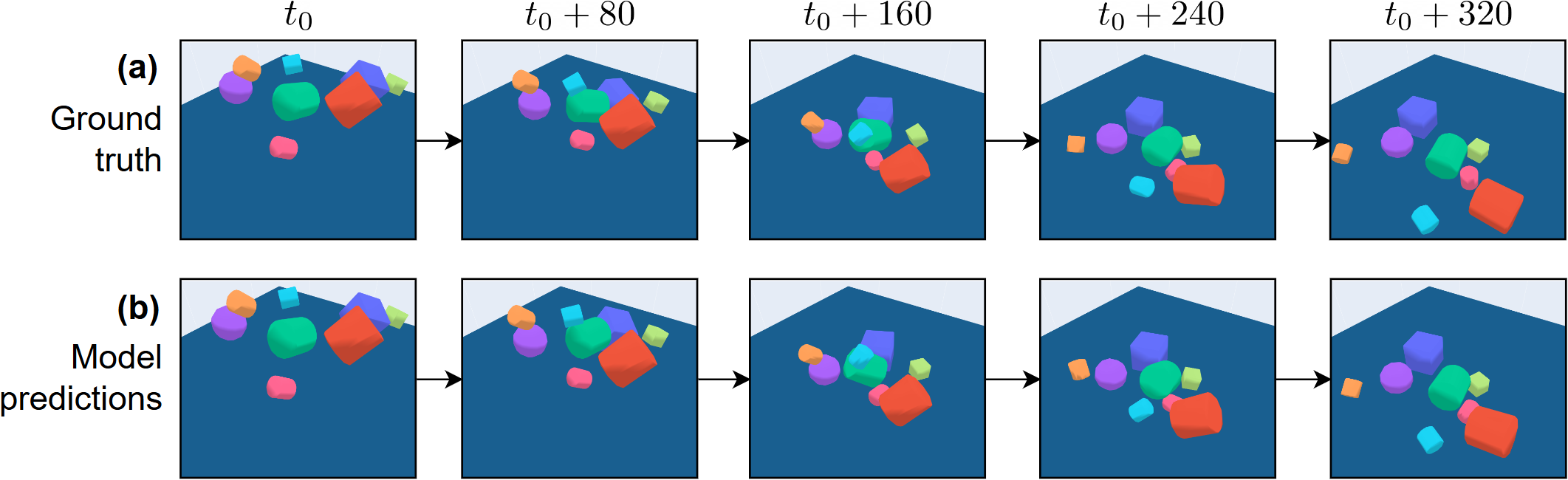
Figure 5: Rollout example on the MoVi-A dataset. (a) Ground truth ; (b) Model predictions. Our model makes very accurate and realistic predictions on the trajectories of rigid bodies despite complex multi-objects collisions and long rollout durations.

HOPNet is designed to predict the forward dynamics of all dynamic objects within a scene. Specifically, HOPNet outputs per-node and per-object accelerations $\hat{\ddot{\bm{x}}}_{i}$, which are then integrated using a second-order forward-Euler method with a timestep $\Delta t=1$ to compute the next positions $\hat{\bm{x}}_{i}^{t+1}$ using the previous and current positions $\bm{x}_{i}^{t-1}$ and $\bm{x}_{i}^{t}$. This integration step is formalized in Eq. 1:

$$\hat{\bm{x}}_{i}^{t+1}=\hat{\ddot{\bm{x}}}^{t}_{i}+2\bm{x}_{i}^{t}-\bm{x}_{i}^{t-1}$$ (1)

3 Results

3.1 Forward dynamics in increasingly complex scenarios

To demonstrate the effectiveness of our framework, we evaluate its performance on the task of learning forward dynamics for interacting rigid objects. Specifically, the objective is to accurately learn object interactions and collisions, and to predict the evolution of their positions and orientations.

We conduct our evaluations using three benchmark video datasets of increasing complexity: MoVi-spheres, MoVi-A, and MoVi-B kubric . Each experiment consists of a video where a set of rigid objects interact within an environment with unknown characteristics – such as gravity and air resistance – that can only be inferred from observations. The MoVi-spheres dataset consists solely of spherical objects, while the MoVi-A includes a mixture of cubes, spheres, and cylinders. The most complex, MoVi-B, contains real-world everyday objects, such as cones and teapots. In each experiment, between 3 to 10 objects are randomly selected, each assigned varying physical parameters (e.g. size, mass, friction). The objects are initialized with random positions and velocities and then released onto a flat surface to simulate dynamic interactions. Detailed descriptions of the datasets are provided in Supplementary Information Sec. 2.1.

We test our framework in an autoregressive manner: the predicted acceleration $\hat{\ddot{\bm{x}}}^{t}$ at time $t$ is used to compute the next position $\hat{\bm{x}}^{t+1}$, which is subsequently fed back as input to predict $\hat{\bm{x}}^{t+2}$, as elaborated in Sec. 2.1. To evaluate the framework’s performance over both short-term and long-term predictions, we consider different rollout horizons $T$ ranging from $25$ to $100$ steps. Our primary results are presented in Fig. 4 for a rollout horizon of $T=50$, aligning with the reported results by the current state-of-the-art baseline models FIGNet fignet and MeshGraphNet meshgraphnet , due to the absence of reproducible code for these models. For a more comprehensive analysis across various horizons $T=\{25,50,75,100\}$, please refer to Supplementary Information Sec. 3.1.

The results presented in Fig. 4 demonstrate that our framework effectively learns and predicts the dynamics of interacting rigid bodies with remarkable accuracy, closely aligning with the ground truth. In line with previous research studies, we report the average Root Mean Square Error (RMSE) for both object positions (Fig. 4a) and orientations (Fig. 4b) after 50 timesteps. On the MoVi-A dataset, our framework achieves high fidelity in capturing both the translational and rotational motions of rigid bodies. Moreover, on the more complex MoVi-B dataset, which includes a diverse set of real-world objects, our framework effectively handles collisions, maintaining robust performance despite the increased complexity. Across all datasets, our method consistently outperforms both state-of-the-art methods MeshGraphNet meshgraphnet and FIGNet fignet by a substantial margin, demonstrating the effectiveness of our higher-order representations and physics-informed inductive biases.

Importantly, our method is capable of performing $50\%$ more rollout steps before reaching the same translational and rotational errors. The best baseline reaches an RMSE of $0.115$ [m] at 50 steps on the MoVi-A dataset, whereas our framework reaches this value after 75 steps. This significant improvement allows more accurate predictions further into the future, supporting better and more robust decision-making in dynamic scenarios. For further analysis of extended rollout horizons, please refer to Sec. 3.1. in the Supplementary Information.

Figure 6: Counterfactual rollout example. (a) Original experiment ; (b) Altered experiment with one sphere removed, shown as a black skeleton to ease understanding. With our dynamic and flexible higher-order topological representation of the environment, our model can easily accommodate any changes in initial conditions: position, orientation, velocity, material properties, …

To further validate the robustness and precision of our framework, we present a challenging multi-object rollout example in Fig. 3. In this scenario, the final positions $\hat{\bm{x}}$ and orientations $\hat{\bm{q}}$ of all objects closely match the ground truth trajectories, highlighting the framework’s precision and robustness in handling complex interactions among multiple entities.

3.2 Counterfactual capabilities and generalization

In addition to the high accuracy of our framework, two critical benefits arise from our design choices. First, the higher-order topological representation of the environment facilitates the modification of initial conditions, enabling the exploration of counterfactual scenarios. Counterfactual scenarios refer to hypothetical situations that differ from the actual conditions, allowing researchers to assess potential outcomes by altering specific variables such as an object’s starting position or mass. These scenarios are inherently challenging because they require the model to accurately predict the effects of changes in initial conditions on the system’s subsequent dynamics, often involving complex and nonlinear interactions. For example, we can investigate questions like: "What if an object had a different starting position?" or "What if it had a different mass?". All scene parameters – including any object’s position, orientation, velocity, mass, and material properties – are fully configurable. Fig. 4 illustrates this flexibility with a counterfactual scenario where a large sphere, initially interacting with multiple objects, is removed at time $t_{0}$. Consequently, the dynamic interactions among the remaining objects evolve differently, leading to a distinct outcome. This counterfactual capability is particularly valuable for decision-making, as it enables the exploration of multiple hypotheses before committing to a specific course of action.

Building on this flexibility, our framework also demonstrates exceptional robustness and generalization capabilities. This second benefit is closely related to the robustness of our model and its capacity to handle out-of-distribution scenarios. By embedding physics-informed message passing into our framework, we enable it to learn fundamental physical laws and effectively extrapolate to unseen complex object geometries. To validate this capability, we trained three models – S, A, and B – on the MoVi-spheres, MoVi-A, and MoVi-B datasets, respectively. Each model was exposed to a different level of object complexity: S only to spheres, A to basic shapes (including spheres), and B to real-world objects (including basing shapes). We then evaluated each model’s generalization performance across all datasets. The results, summarized in Fig. 7, demonstrate that HOPNet generalizes very effectively to unseen object geometries. Despite being trained solely on spherical objects, model S achieves competitive and even superior performance on MoVi-A and MoVi-B than models A and B (Fig. 7a and 7b). This exceptional generalization ability can be attributed to model’s S exposure to a more diverse range of collision scenarios. In contrast to models A and B, which primarily encountered static and slow-speed interactions, model S was exposed to more dynamic and varied collisions (Fig. 7c). This difference in variety can be explained by the nature of each dataset’s objects: spheres remain in continuous motion, while more complex shapes like cubes or cylinders tend to stabilize on one of their faces, leading to fewer and more similar interactions overall.

In summary, this analysis demonstrates HOPNet’s superior ability to generalize to unseen complex geometries and emphasizes the importance of having a large variety of operating conditions in a dataset. An example of this generalization is presented in Supplementary Information Sec. 3.2.

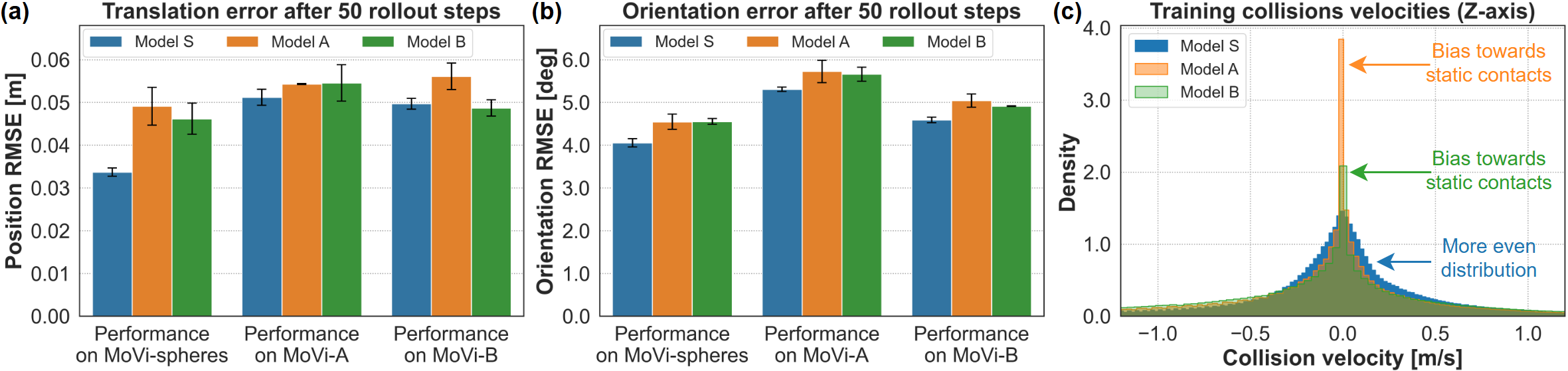
Figure 7: Generalization performance of HOPNet. (a) Translation and (b) orientation errors after $T=50$ rollout steps of three different models – S, A, and B – trained on MoVi-spheres, MoVi-A, and MoVi-B respectively. Error bars indicate the minimum, mean, and maximum performance across three independent random seeds. (c) Distribution of the collision velocities encountered by each model during training. Model S, trained solely on spherical objects, generalizes effectively to more complex object geometries in MoVi-A and MoVi-B. This ability arises from model S’s exposure to a wider range of collision dynamics compared to the slower and more static collisions seen by models A and B. Further details about the datasets are available in Supplementary Information Sec. 2 and 3.

3.3 Importance of physical consistency

To further demonstrate the impact of our core contributions, we conducted ablation studies on both the higher-order topological representation and the physics-informed inductive biases. For the topological representation, we compared our full higher-order representation against a version that omits the higher-order object-level cells $X^{(4)}$. We did not explicitly test the removal of other higher-order cells, as existing baselines MeshGraphNet meshgraphnet and FIGNet fignet can be considered approximations of reduced representations without mesh triangles $X^{(2)}$ and object-level cells $X^{(4)}$, respectively. To assess the importance of physics-informed biases, we performed two key modifications:(1) omitting key information inside the node features $\bm{h}^{(0)}$, specifically the relative distance between the node and the object’s center of mass, and (2) removing the multi-step sequential message-passing. Further architectural details about the models used in these ablation experiments are provided in Supplementary Information Sec. 3.3.

When comparing our full combinatorial complex representation to its ablated versions, Fig. 8a reveals that removing the object-level cells $X^{(4)}$ leads to a significant drop in performance, with a translation RMSE $44.4\%$ larger than the default HOPNet framework. This decline is expected since intra-object messages are restricted to node-to-node communication, which diminishes the model’s expressiveness and fails to capture the rigidity of each object. Although a virtual node is added at the center of each object to enhance multi-hop communication between nodes, the lack of physical consistency results in a noticeable reduction in accuracy. This modified version resembles FIGNet fignet in its features but still retains the physics-informed message-passing from HOPNet. With the performance of this ablated model ($\text{RMSE}^{\text{pos}}=0.078$ [m]) falling in between HOPNet ($\text{RMSE}^{\text{pos}}=0.054$ [m]) and FIGNet ($\text{RMSE}^{\text{pos}}=0.115$ [m]), this study also demonstrate the benefits of HOPNet’s physics-informed message-passing compared to a standard convolutional one.

Beyond our topological representation, our second key contribution is the incorporation of physics-informed biases within our topological neural network. To underscore the importance of feature selection, we tested the removal of a critical attribute from the node cell features $\bm{h}^{(0)}$: the relative distance between the node and the object’s center of mass. This feature is particularly important from a physics standpoint, as it provides structural information about the object and enables the prediction of how collisions near specific nodes affect the object’s overall momentum. To evaluate the significance of this feature, we tested our full framework and its simplified version on two datasets: MoVi-spheres and MoVi-A. In the MoVi-spheres dataset, which consists exclusively of spherical objects, removing the "center-mass distance" feature is expected to have a minimal impact, as a sphere’s moment of inertia is uniform in all directions. In contrast, the cubes and cylinders in MoVi-A possess anisotropic moments of inertia, making the nodes’ distances to the center of mass critical for accurately predicting collisions with these objects.

The results presented in Fig. 8b validate our hypothesis. We only observe a slight performance decline on the MoVi-spheres dataset with $\text{RMSE}^{\text{pos}}$ increasing from $0.034$ [m] to $0.040$ [m], primarily due to the coarse resolution of the spherical meshes. In contrast, there is a substantial drop in accuracy on the MoVi-A dataset, highlighting the critical importance of physics-informed biases for accurately modeling objects with more complex shapes. The $\text{RMSE}^{\text{pos}}$ becomes $26\%$ larger at $0.068$ [m] compared to $0.054$ [m] for the default model. Additionally, on both datasets, the seed-to-seed variability (shown by the error bars) greatly increases compared to the default HOPNet model, underscoring the robustness of our approach.

Figure 8: Importance of physical consistency in HOPNet. (a) Ablation study on higher-order topological representations; (b) Ablation study on physics-based features; (c) Ablation study on physics-informed message-passing. Error bars indicate the minimum, mean, and maximum performance across three independent random seeds.

Finally, we assess the impact of embedding physics-informed inductive biases within our message-passing scheme. Specifically, we compare our physics-informed sequential message-passing (illustrated in Fig. 2) with a non-sequential version, where information flows freely between all cells without any structural guidance. This alternative approach removes the inductive bias that constrains the transfer pathways within our topological neural network. The results, presented in Fig. 8c, clearly demonstrate that without these guided pathways, the model struggles to efficiently learn collision dynamics and has difficulty capturing the interactions among higher-order groups. The $\text{RMSE}^{\text{pos}}$ increases to $0.061$ [m], even though this variant of the model contains $34\%$ more learnable parameters than the default HOPNet. This highlights the critical role of structured information flow in modeling and learning complex physical interactions.

3.4 Hyperparameter robustness and efficiency

Our framework demonstrates significant robustness to variations in hyperparameter selection, highlighting its efficiency and generalizability across diverse applications. When testing a smaller variant of HOPNet by reducing the total number of learnable parameters by $74\%$ through a decreased hidden embedding size, we observed only a minor decrease in performance. This finding confirms the framework’s efficiency in learning rigid-body interactions. Additionally, increasing the total number of message-passing steps leads to improved accuracy, a trend consistent with conventional GNNs. A detailed analysis of model size effects is provided in Supplementary Information Sec. 3.4.

Moreover, our framework shows minimal sensitivity to critical modeling hyperparameters, such as the collision radius $d_{c}$ used to define collision contact cells $X^{(3)}$. Performance remained stable even when the collision radius was halved or doubled, further validating the method’s stability across a wide range of hyperparameter values. This robustness minimizes the need for extensive fine-tuning, thereby broadening our framework’s applicability across different tasks and scenarios. Additional details on this analysis can be found in Supplementary Information Sec. 3.5.

4 Discussion

In this work, we introduced a novel topology-based framework for modeling rigid bodies and learning their dynamics, addressing critical limitations in existing approaches. By incorporating higher-order topology groups and leveraging physics-informed inductive biases, our framework achieves superior accuracy in predicting complex collisions and interactions between rigid objects. The core strength of our approach lies in its alignment with real-world physics, where we employ domain knowledge to enhance data modeling and design a neural architecture operating on these higher-order structures.

To the best of our knowledge, HOPNet is the first framework to employ higher-order topology groups for modeling spatiotemporal dynamic systems and performing regression instead of classification. Our method demonstrates significant improvements over state-of-the-art baseline models in capturing highly nonlinear dynamics, learning purely from observations. These results highlight the potential of applying higher-order topological representations to other geometric learning tasks, particularly for multi-entity systems governed by known physical laws or structured graph-based data.

We validated our approach on a range of increasingly complex datasets, from simple shapes to real-world objects with intricate geometries. In addition to outperforming baseline models, our framework demonstrated robust generalization to unseen scenarios and the ability to address counterfactual questions – an essential feature for decision-making in dynamic systems. Although this work focuses on rigid-body dynamics, the framework is adaptable enough to extend to deformable objects, such as soft bodies or fluids, and to incorporate additional forces like magnetic or electric fields.

While our framework requires additional effort to represent scenes using combinatorial complexes compared to simpler graph-based methods, the resulting enhanced accuracy and learning efficiency underscore the value of this increased complexity. In particular, the integration of physics-informed message-passing enables more accurate predictions than standard GNNs and offers greater robustness to hyperparameter selection. This robustness facilitates the broad generalization of our framework across a wide range of diverse tasks.

Nevertheless, scaling our method to extremely complex meshes with millions of faces remains a challenge. While downsampling or mesh approximation could mitigate the computational load, alternative methods using implicit surface modeling might be better suited for such extreme cases.

Finally, while our framework currently relies on explicit state information (e.g. geometry, mass, friction) for counterfactual reasoning and generalization, possible extensions could infer these parameters implicitly from data – past observations – in other environments. Additionally, coupling our model with visual perception systems is a promising direction for further exploration, enabling learning directly from raw pixel data.

In summary, our framework effectively models rigid-body dynamics by integrating topological representations with physics-informed neural architectures. Our findings are consistent with recent research that underscores the critical role of higher-order representations in enhancing both the efficiency and accuracy of deep learning models for complex systems. By leveraging these advanced representations, our approach not only aligns with but also advances the current understanding of how deep learning can effectively tackle intricate dynamic interactions.

5 Methods

5.1 Representation of rigid body systems

We introduce a novel representation for environments comprising $K$ interacting rigid bodies. As previously discussed, current methods typically utilize standard graphs $\mathcal{G}=(\mathcal{V},\mathcal{E})$, where vertices $\mathcal{V}$ represent nodes and edges $\mathcal{E}$ denote connections between them. In these approaches, the mesh $M$ of each object, defined by its node positions $\{\bm{x}_{i}\}_{i=1..N}$ and faces $\{f_{j}\}_{j=1..F}$, is integrated into a global graph $\mathcal{G}$. However, this integration leads to the loss of essential structural information, as standard graphs are unable to explicitly define faces and individual objects. Consequently, the detailed geometries and specific interactions of rigid bodies are not accurately captured, thereby limiting the effectiveness of these conventional graph-based methods.

In contrast, our framework leverages a combinatorial complex $\mathcal{X}^{t}$ to model the entire environment at a given time $t$. This complex enables us to explicitly define a hierarchy of higher-order node groups, referred to as cells $X^{(r)}$. Each cell of rank $r$ possesses associated features $\bm{h}^{(r)}$ and can exchange messages with other groups of the same or different ranks. This higher-order representation enables a more precise encoding of both object structure and interactions, ensuring that no critical geometric or topological information is lost during the modeling process.

Our framework defines five distinct types of cells to comprehensively capture the dynamics and interactions of rigid bodies: nodes $X^{(0)}$, edges $X^{(1)}$, mesh triangles $X^{(2)}$, collision contacts $X^{(3)}$, and objects $X^{(4)}$. The cells $X^{(0)}$ and $X^{(1)}$ correspond directly to the nodes $\mathcal{V}$ and edges $\mathcal{E}$ of a conventional graph $\mathcal{G}=(\mathcal{V},\mathcal{E})$. To accurately capture the geometric structure of each object, we introduce $X^{(2)}$ cells to represent individual mesh triangles, and $X^{(4)}$ cells to represent entire objects. Furthermore, to model collisions and enable interactions between individual objects, we incorporate collision contacts $X^{(3)}$. These $X^{(3)}$ cells link two mesh triangles $X^{(2)}$ from different objects when they come within a specified collision radius $d_{c}$. This combinatorial complex representation $X^{t}$, alongside the traditional graph representation $\mathcal{G}^{t}$, is illustrated in Fig. 1.

Node features $\bm{h}^{(0),\text{features}}$ for node $i$ belonging to object $k$ consist of two key components: (1) finite-difference velocities derived from the node’s positional history; and (2) center-mass distances between a node and its object’s center of mass. They are formalized in Eq. 2:

$$\bm{h}^{(0),\text{features}}_{i}=[\dot{\bm{x}}_{i}^{t},\lVert\dot{\bm{x}}_{i}^{t}\rVert,\dot{\bm{x}}_{i}^{t-1},\lVert\dot{\bm{x}}_{i}^{t-1}\rVert,\bm{d}^{t_{0}}_{i},\lVert\bm{d}^{t_{0}}_{i}\rVert,\bm{d}^{t}_{i},\lVert\bm{d}^{t}_{i}\rVert]$$ (2)

$$\dot{\bm{x}}^{t}_{i}=\bm{x}^{t}_{i}-\bm{x}^{t-1}_{i}\qquad\bm{d}_{i}^{t}=\bm{x}^{t}_{i}-\bm{x}^{t}_{k}$$

where $\dot{\bm{x}}^{t}_{i}$ and $\dot{\bm{x}}^{t-1}_{i}$ are the finite-difference velocities at time $t$ and $t-1$, $\bm{x}_{i}^{t}$ is the position of node $i$ at time $t$, $\bm{x}_{k}^{t}$ is the position of object $k$ at time $t$, $\bm{d}^{t}_{i}$ and $\bm{d}^{t_{0}}_{i}$ are the center-mass distances at time time $t$ and $t_{0}$, $[]$ indicates concatenation and $\lVert\rVert$ is the Euclidean norm.

Edge features $\bm{h}^{(1),\text{features}}_{s\rightarrow r}$ between sender node $s$ and receiver node $r$ include the node-to-node distances measured at time $t_{0}$ and current time $t$, leading to Eq. 3:

$$\bm{h}^{(1),\text{features}}_{s\rightarrow r}=[\bm{x}^{t_{0}}_{s}-\bm{x}^{t_{0}}_{r},\lVert\bm{x}^{t_{0}}_{s}-\bm{x}^{t_{0}}_{r}\rVert,\bm{x}^{t}_{s}-\bm{x}^{t}_{r},\lVert\bm{x}^{t}_{s}-\bm{x}^{t}_{r}\rVert]$$ (3)

where $\bm{x}^{t}_{s}$ and $\bm{x}^{t_{0}}_{s}$ are the positions of sender node $s$ at time $t$ and $t_{0}$, and $\bm{x}^{t}_{r}$ and $\bm{x}^{t_{0}}_{r}$ are the positions of receiver node $r$ at time $t$ and $t_{0}$.

Mesh triangle features $\bm{h}^{(2),\text{features}}$ include the normal vector of each mesh triangle $i$:

$$\bm{h}_{i}^{(2),\text{features}}=[\bm{n}_{i}^{t},\lVert\bm{n}_{i}^{t}\rVert]$$ (4)

where $\bm{n}_{i}^{t}$ is the normal vector vector of mesh triangle $i$ at time $t$.

Collision contact features $\bm{h}^{(3),\text{features}}_{s\rightarrow r}$ between sender triangle $s$ and receiver triangle $r$ are defined by first computing the closest points $\bm{p}_{s}$ and $\bm{p}_{r}$ on each respective triangle. The collision direction is captured by the relative vector $\bm{p_{s}}-\bm{p_{r}}$. Subsequently, a three-axis local coordinate system is established around the closest points on each triangle, utilizing their three vertices $\{s_{j}\}_{j=1,2,3}$ and $\{r_{j}\}_{j=1,2,3}$. This structured approach, formalized in Eq. 5, ensures precise modeling of collision dynamics by accurately representing the spatial relationships between interacting mesh triangles:

$$\bm{h}^{(3),\text{features}}_{s\rightarrow r}=[\bm{p}_{s}^{t}-\bm{p}_{r}^{t},\lVert\bm{p}_{s}^{t}-\bm{p}_{r}^{t}\rVert,[\bm{x}_{s_{j}}^{t}-\bm{p}_{s}^{t},\lVert\bm{x}_{s_{j}}^{t}-\bm{p}_{s}^{t}\rVert]_{j=1,2,3},[\bm{x}_{r_{j}}^{t}-\bm{p}_{r}^{t},\lVert\bm{x}_{r_{j}}^{t}-\bm{p}_{r}^{t}\rVert]_{j=1,2,3}]$$ (5)

where $\bm{p}_{s}$ is the closest point to triangle $r$ on triangle $s$, $\bm{p}_{r}$ is the closest point to triangle $s$ on triangle $r$, $\{\bm{x}^{t}_{s_{j}}\}_{j=1,2,3}$ are the positions of all three vertices of triangle $s$ and $\{\bm{x}^{t}_{r_{j}}\}_{j=1,2,3}$ are the positions of all three vertices of triangle $r$.

Object features $\bm{h}^{(4),\text{features}}$ for object $k$ include finite-difference velocities computed at the object’s center of mass. Additionally, a one-hot encoded vector $\bm{b}$ distinguishes between static objects and dynamic objects. Finally, some of the object’s physical parameters are also included:

$$\bm{h}^{(4),\text{features}}_{k}=[\dot{\bm{x}}_{k}^{t},\lVert\dot{\bm{x}}_{k}^{t}\rVert,\dot{\bm{x}}_{k}^{t-1},\lVert\dot{\bm{x}}_{k}^{t-1}\rVert,\bm{b},m,c_{1},c_{2}]$$ (6)

where $\dot{\bm{x}}^{t}_{k}$ and $\dot{\bm{x}}^{t-1}_{k}$ are the finite-difference velocities at time $t$ and $t-1$, $\bm{b}$ is the one-hot encoded object type, $m$ is the object’s mass, $c_{1}$ the friction coefficient and $c_{2}$ the restitution coefficient.

This combinatorial complex representation $\mathcal{X}^{t}$ is inherently translation-invariant, as none of the cell features $\bm{h}^{(r)}$ include the absolute positions of nodes $\{\bm{x}_{i}\}_{i=1..N}$ or objects $\{\bm{x}_{k}\}_{k=1..K}$. This design ensures a translation-equivariant framework, enhancing the model’s generalization capabilities.

5.2 Physics-informed message passing

After constructing a combinatorial complex $\mathcal{X}$ to accurately represent rigid bodies, we design a neural architecture that directly operates on this topological structure. Standard message-passing Graph Neural Networks (GNNs) gnn are inadequate for processing higher-order node groups. Instead, we introduce a message-passing Topological Neural Network (TNN) topological_deep_learning , which efficiently exchanges information between cells of varying ranks. To ensure consistency and clarity, we adopt the terminology and notations introduced by topological_deep_learning , avoiding the need to redefine conventions.

To introduce how message-passing operates between different $X^{(r)}$ cells, we can compare it to graph-based message-passing, which is a specific case of topological message-passing. In a graph $\mathcal{G}$, a message is sent from a node $v_{1}$ to another node $v_{2}$ if an edge $e_{v_{1}\rightarrow v_{2}}$ exists. Additionally, if edges also have embeddings, nodes $v_{1}$ and $v_{2}$ can send messages to the edge $e_{v_{1}\rightarrow v_{2}}$. Hence, in graph message-passing, the edges $\mathcal{E}$ define the neighborhood of nodes and their ability to communicate.

Figure 9: Physics-informed message passing. (a) Enhancing mesh face cells $X^{(2)}$ embeddings with nodes, edges, and object cells; (b) Computing the effect of a collision from two mesh faces $s$ and $r$ on each other; (c) Updating triangles $s$ and $r$ after collisions.

In a combinatorial complex, the neighborhoods $\{\mathcal{N}\}$ of a cell $x^{(r)}$ also define its ability to exchange messages with other cells. Unlike graphs, a cell $x^{(r)}$ has multiple neighborhoods, as neighboring cells can have a lower, same, or higher rank. The $k$-up neighborhood function $\mathcal{N}_{\nearrow,k}(x)$ of a cell $x$ is defined as the set $\{y\in\mathcal{X}|x\subsetneq y,\text{rk}(y)=\text{rk}(x)+k\}$ where $\text{rk}(x)$ is the "rank function", returning the rank $r$ of cell $x^{(r)}$. Similarly, the $k$-down neighborhood function $\mathcal{N}_{\searrow,k}(x)$ of a cell $x$ is defined as the set $\{y\in\mathcal{X}|y\subsetneq x,\text{rk}(y)=\text{rk}(x)-k\}$.

Leveraging neighborhood functions, we construct a message-passing neural architecture operating on the combinatorial complexes $\{\mathcal{X}^{t}\}$. Our architecture follows an Encode-Process-Decode graph_network_simulator paradigm. In the encoding step, the cell features $\bm{h}^{(r),\text{features}}$ are passed through separate Multi-Layer Perceptrons (MLPs), one for each cell rank:

$$\bm{h}^{(r)}=\text{MLP}^{\text{encoder}}_{r}(\bm{h}^{(r),\text{features}})\vspace{-0.1cm}$$ (7)

The processing step is where sequential message-passing occurs. While the topological representation $\mathcal{X}$ and the neighborhood functions $\mathcal{N}(x)$ offer significant flexibility, theoretically supporting learnable messages between all cell ranks, this approach would introduce unnecessary complexity, computational overhead, and negatively impact the learning efficiency of the network. Therefore, it is essential to carefully constrain message-passing pathways, guiding the information flow to only relevant neighboring cells. To define these pathways, we use physics knowledge about collisions and create a sequential message-passing structure, visible in Fig. 3b.

The message-passing used in HOPNet can be divided into three main parts: (A) enhancing mesh faces with intra-object data to prepare for collisions; (B) processing inter-object collisions using mesh faces; (C) updating individual objects and nodes. These three main parts are outlined in Fig. 3b.

A. Enhancing mesh faces with intra-object data. In this first part, the embeddings of $X^{(2)}$ cells are enhanced with messages from nodes $X^{(0)}$ using $\mathcal{N}_{\searrow,2}(x)$, edges $X^{(1)}$ using $\mathcal{N}_{\searrow,1}(x)$, and object $X^{(4)}$ cells using $\mathcal{N}_{\nearrow,2}(x)$. This first main part integrates critical information into the mesh triangles’ embeddings $X^{(2)}$, which are later used to process the inter-object collisions. It is visually illustrated in Fig. 9a, while the messages are formally defined in Eq. 8, and the aggregation in Eq. 9:

$$\bm{m}_{j}^{0\rightarrow 2}=\text{MLP}^{\text{processor}}_{m0\rightarrow 2}(\bm{h}_{j}^{(0)})\quad\bm{m}_{j}^{1\rightarrow 2}=\text{MLP}^{\text{processor}}_{m1\rightarrow 2}(\bm{h}_{j}^{(1)})\quad\bm{m}_{j}^{4\rightarrow 2}=\text{MLP}^{\text{processor}}_{m4\rightarrow 2}(\bm{h}_{j}^{(4)})$$ (8)

$$\bm{h}^{\prime(2)}_{i}=\text{MLP}^{\text{processor}}_{2}([\bm{h}_{i}^{(2)},\sum_{\forall j\in\mathcal{N}_{\searrow,2}(x_{i}^{(2)})}\bm{m}_{j}^{0\rightarrow 2},\sum_{\forall j\in\mathcal{N}_{\searrow,1}(x_{i}^{(2)})}\bm{m}_{j}^{1\rightarrow 2},\sum_{\forall j\in\mathcal{N}_{\nearrow,2}(x_{i}^{(2)})}\bm{m}_{j}^{4\rightarrow 2}])$$ (9)

where $\bm{m}^{0\rightarrow 2}$, $\bm{m}^{1\rightarrow 2}$, and $\bm{m}^{4\rightarrow 2}$ are learnable messages – sent from nodes, edges, and object cells to mesh triangles respectively – and $\bm{h}^{\prime(2)}$ are the new mesh triangle embeddings after this message-passing step.

B. Processing inter-object collisions using mesh faces. This second major part, particularly critical in our framework as it models the inter-object collisions, is presented in Fig. 9b and 9c. To ensure energy conservation during each individual collision between two mesh triangles $x_{s}^{(2)}$ and $x_{r}^{(2)}$, the messages $m^{2\rightarrow 2}_{s\rightarrow r}$ and $m^{2\rightarrow 2}_{r\rightarrow s}$ are built in a permutation-invariant manner using the unidirectional collision contacts cells $x^{(3)}_{s\rightarrow r}$ and $x^{(3)}_{r\rightarrow s}$. First, the collision effect from $x^{(2)}_{s}$ on $x^{(2)}_{r}$ is computed using $x^{(3)}_{s\rightarrow r}$ (step 2, Eq. 10). Then, the new embedding $\bm{h}^{\prime\prime(2)}_{r}$ of the receiver triangle $x^{(2)}_{r}$ is calculated by aggregating all incoming collision messages on this mesh triangle (step 3, Eq. 11), leading to:

$$\bm{m}_{s}^{2\rightarrow 3}=\text{MLP}^{\text{processor}}_{m2\rightarrow 3}(\bm{h}_{s}^{\prime(2)})\qquad\bm{h}^{\prime(3)}_{s\rightarrow r}=\text{MLP}^{\text{processor}}_{3}([\bm{h}_{s\rightarrow r}^{(3)},\bm{m}_{s}^{2\rightarrow 3},\bm{m}_{r}^{2\rightarrow 3}])$$ (10)

$$\bm{m}_{s\rightarrow r}^{3\rightarrow 2}=\text{MLP}^{\text{processor}}_{m3\rightarrow 2}(\bm{h}_{s\rightarrow r}^{\prime(3)})\qquad\bm{h}^{\prime\prime(2)}_{r}=\text{MLP}^{\text{processor}}_{2^{\prime}}([\bm{h}_{r}^{\prime(2)},\sum_{\forall j\in\mathcal{N}_{\nearrow,1}(x^{(2)}_{r})}\bm{m}_{j\rightarrow r}^{3\rightarrow 2}])$$ (11)

where $\bm{m}_{s}^{2\rightarrow 3}$ and $\bm{m}_{r}^{2\rightarrow 3}$ are learnable messages from sender triangle $s$ and receiver triangle $r$, $\bm{h}^{\prime(3)}_{s\rightarrow r}$ is the updated collision contact embedding after message-passing step 2, $\bm{m}_{s\rightarrow r}^{2\rightarrow 3}$ is a learnable message from the collision contact $x^{(3)}_{s\rightarrow r}$ to the receiver triangle $x^{(2)}_{r}$, and $\bm{h}^{\prime\prime(2)}$ are the new mesh triangle embeddings after message-passing step 3.

C. Updating intra-objects cells after collisions. This part handles the intra-object updates by integrating the effects of incoming collisions and the current velocity and momentum. The information about incoming collisions is embedded in the updated triangle features $\bm{h}^{\prime\prime(2)}$, while the velocity and momentum at time $t$ are encoded in the node embeddings $\bm{h}^{(0)}$ and object embeddings $\bm{h}^{(4)}$. In step 4 (Eq. 12), updated object embeddings $\bm{h}^{\prime(4)}$ are computed using the incoming collisions. Subsequently, the final object embeddings $\bm{h}^{\prime\prime(4)}$ and node embeddings $\bm{h}^{\prime(0)}$ are derived (Eq. 13-15), where $k$ is the index of the object containing node $i$ and $N$ is the total number of nodes in object $k$.

$$\bm{m}_{i}^{2\rightarrow 4}=\text{MLP}^{\text{processor}}_{m2\rightarrow 4}(\bm{h}_{i}^{\prime\prime(2)})\qquad\bm{h}^{\prime(4)}_{i}=\text{MLP}^{\text{processor}}_{4}([\bm{h}_{i}^{(4)},\sum_{\forall j\in\mathcal{N}_{\searrow,2}(x^{(4)}_{i})}\bm{m}_{j}^{2\rightarrow 4}])$$ (12)

$$\bm{m}_{i}^{0\rightarrow 4}=\text{MLP}^{\text{processor}}_{m0\rightarrow 4}(\bm{h}_{i}^{(0)})\qquad\bm{m}_{i}^{4\rightarrow 0}=\text{MLP}^{\text{processor}}_{m4\rightarrow 0}(\bm{h}_{i}^{\prime\prime(4)})$$ (13)

$$\bm{h}^{\prime(0)}_{i}=\text{MLP}^{\text{processor}}_{0}([\bm{h}_{i}^{(0)},\bm{m}_{k}^{4\rightarrow 0}])$$ (14)

$$\bm{h}^{\prime\prime(4)}_{n}=\text{MLP}^{\text{processor}}_{4^{\prime}}([\bm{h}_{n}^{(0)},\frac{1}{N}\sum_{\forall j\in\mathcal{N}_{\searrow,4}(x^{(4)}_{n})}\bm{m}_{j}^{0\rightarrow 4}])$$ (15)

where $\bm{m}^{2\rightarrow 4}$ are learnable messages from mesh triangles to their parent object, $\bm{h}_{i}^{\prime(4)}$ are the new object embeddings after message-passing step 4, $\bm{m}^{0\rightarrow 4}$ are learnable messages from nodes to object cells, $\bm{m}^{4\rightarrow 0}$ are learnable messages from object to node cells, $\bm{h}^{\prime(0)}$ the final node embeddings, and $\bm{h}^{\prime\prime(4)}$ the final object embeddings after message passing step 5.

D. Predicting accelerations and the next pose. This last part contains the final decoding step of our Encode-Process-Decode architecture (step 6). It simply consists of a readout step on the object embeddings $\bm{h}^{\prime\prime(4)}$ and node embeddings $\bm{h}^{\prime(0)}$ with two MLPs (Eq. 16).

$$\hat{\ddot{\bm{x}}}_{i}=\text{MLP}^{\text{decoder}}_{0}(\bm{h}_{i}^{\prime(0)})\qquad\hat{\ddot{\bm{x}}}_{n}=\text{MLP}^{\text{decoder}}_{4}(\bm{h}_{i}^{\prime\prime(4)})$$ (16)

where $\hat{\ddot{\bm{x}}}_{i}$ and $\hat{\ddot{\bm{x}}}_{n}$ are the predicted accelerations for nodes and objects, respectively.

Finally, the last element of our framework consists in predicting the poses of all objects at time $t+1$. It is exclusively applied during inference, not training. Here, we use the second-order forward-Euler integration to predict the next node positions $\hat{\bm{x}}^{t+1}_{i}$. To ensure the objects maintain their rigidity over extended rollouts, we use shape_matching . Using the predicted node positions $\{\hat{\bm{x}}_{i}\}_{i=1..N}$ of each object $k$, we compute the updated center of mass $\hat{\bm{x}}^{t+1}_{k}$ and quaternion orientation $\hat{\bm{q}}^{t+1}_{k}$ for each object. Finally, we apply the rotation $\hat{\bm{q}}^{t+1}_{k}$ then translation $\hat{\bm{x}}^{t+1}_{k}$ to the reference mesh $M$, and obtain the final node positions predictions.

5.3 Performance evaluation metrics

We use the Root Mean Square Error (RMSE) between the predicted and ground truth object trajectories, on both position and rotation. We report the average RMSE per object in meters (for position) and degrees (for rotation). The exact formulas are given in Eq. 17 and 18, where $\langle\bm{q}\rangle$ is the norm of the vector part of quaternion $\bm{q}$ and $\times$ is the Hamilton product.

$$\text{RMSE}^{\text{pos}}=\sqrt{\frac{1}{K}\sum_{k=1}^{K}\lVert\hat{\bm{x}}-\bm{x}\rVert^{2}}$$ (17)

$$\text{RMSE}^{\text{ori}}=\sqrt{\frac{1}{K}\sum_{k=1}^{K}\frac{360}{\pi}\arcsin{(\langle\hat{\bm{q}}\times\bm{q}^{-1}\rangle)}}$$ (18)

Data availability

The datasets used for the experiments have been generated with the Kubric library kubric . The exact parameters used to generate the datasets are given in Supplementary Information Sec. 2.

Code availability

The implementation of the proposed method is based on PyTorch pytorch and TopoNetX toponetx . The source code and model checkpoints will be made publicly available on GitHub after acceptance.

Author contributions

A.W. and O.F. conceptualized the idea, A.W. developed the methodology, A.W. and O.F. conceived the experiments, A.W. conducted the experiments, A.W. and O.F. analyzed the results, and A.W. and O.F. wrote the manuscript.

Competing interests

The authors declare no competing interest.

Additional information

Correspondence and requests for materials should be addressed to Olga Fink.

References

- (1) Todorov, E., Erez, T. & Tassa, Y. Mujoco: A physics engine for model-based control. In 2012 IEEE/RSJ International Conference on Intelligent Robots and Systems, 5026–5033 (2012).
- (2) Coumans, E. Bullet physics simulation. In ACM SIGGRAPH 2015 Courses, SIGGRAPH ’15 (Association for Computing Machinery, New York, NY, USA, 2015).
- (3) Smith, R. Open Dynamics Engine (2005). URL https://www.ode.org/.
- (4) Corporation, N. Nvidia PhysX system software (2008). URL https://github.com/NVIDIA-Omniverse/PhysX.
- (5) Pfaff, T., Fortunato, M., Sanchez-Gonzalez, A. & Battaglia, P. W. Learning mesh-based simulation with graph networks. In International Conference on Learning Representations (ICLR) (2021).
- (6) Allen, K. R. et al. Learning rigid dynamics with face interaction graph networks. In International Conference on Learning Representations (ICLR) (2023).
- (7) Parmar, M., Halm, M. & Posa, M. Fundamental challenges in deep learning for stiff contact dynamics. In 2021 IEEE/RSJ International Conference on Intelligent Robots and Systems (IROS), 5181–5188 (2021).
- (8) Piloto, L. S., Weinstein, A., Battaglia, P. & Botvinick, M. Intuitive physics learning in a deep-learning model inspired by developmental psychology. Nature Human Behaviour 6, 1257–1267 (2022).
- (9) Kipf, T. et al. Conditional Object-Centric Learning from Video. In International Conference on Learning Representations (ICLR) (2022).
- (10) Elsayed, G. F. et al. SAVi++: Towards end-to-end object-centric learning from real-world videos. In Advances in Neural Information Processing Systems (2022).
- (11) Singh, G., Wu, Y.-F. & Ahn, S. Simple unsupervised object-centric learning for complex and naturalistic videos. In Koyejo, S. et al. (eds.) Advances in Neural Information Processing Systems, vol. 35, 18181–18196 (Curran Associates, Inc., 2022).
- (12) Wu, Z., Dvornik, N., Greff, K., Kipf, T. & Garg, A. Slotformer: Unsupervised visual dynamics simulation with object-centric models. In International Conference on Learning Representations (ICLR) (2023).
- (13) Burgess, C. P. et al. MONet: Unsupervised scene decomposition and representation (2019). URL https://arxiv.org/abs/1901.11390. 1901.11390.
- (14) Locatello, F. et al. Object-centric learning with slot attention. In Larochelle, H., Ranzato, M., Hadsell, R., Balcan, M. & Lin, H. (eds.) Advances in Neural Information Processing Systems, vol. 33, 11525–11538 (Curran Associates, Inc., 2020).
- (15) Vaswani, A. et al. Attention is all you need. In Guyon, I. et al. (eds.) Advances in Neural Information Processing Systems, vol. 30 (Curran Associates, Inc., 2017).
- (16) Ding, D., Hill, F., Santoro, A., Reynolds, M. & Botvinick, M. Attention over learned object embeddings enables complex visual reasoning. In Advances in Neural Information Processing Systems, vol. 34, 9112–9124 (Curran Associates, Inc., 2021).
- (17) Chen, Z. et al. Comphy: Compositional physical reasoning of objects and events from videos. In International Conference on Learning Representations (ICLR) (2022).
- (18) Bear, D. et al. Physion: Evaluating physical prediction from vision in humans and machines. In Vanschoren, J. & Yeung, S. (eds.) Proceedings of the Neural Information Processing Systems Track on Datasets and Benchmarks, vol. 1 (2021).
- (19) Scarselli, F., Gori, M., Tsoi, A. C., Hagenbuchner, M. & Monfardini, G. The graph neural network model. IEEE transactions on neural networks 20, 61–80 (2008).
- (20) Sanchez-Gonzalez, A. et al. Learning to simulate complex physics with graph networks. In III, H. D. & Singh, A. (eds.) Proceedings of the 37th International Conference on Machine Learning, vol. 119 of Proceedings of Machine Learning Research, 8459–8468 (PMLR, 2020).
- (21) Han, Z., Kammer, D. S. & Fink, O. Learning physics-consistent particle interactions. PNAS Nexus 1, pgac264 (2022).
- (22) Han, J. et al. Learning physical dynamics with subequivariant graph neural networks. In Koyejo, S. et al. (eds.) Advances in Neural Information Processing Systems, vol. 35, 26256–26268 (Curran Associates, Inc., 2022).
- (23) Allen, K. R. et al. Graph network simulators can learn discontinuous, rigid contact dynamics. In Liu, K., Kulic, D. & Ichnowski, J. (eds.) Proceedings of The 6th Conference on Robot Learning, vol. 205 of Proceedings of Machine Learning Research, 1157–1167 (PMLR, 2023).
- (24) Battaglia, P. W. et al. Relational inductive biases, deep learning, and graph networks (2018). URL http://arxiv.org/abs/1806.01261. 1806.01261.
- (25) Oono, K. & Suzuki, T. Graph Neural Networks Exponentially Lose Expressive Power for Node Classification. In International Conference on Learning Representations (ICLR) (2020).
- (26) Battiston, F. et al. The physics of higher-order interactions in complex systems. Nature Physics 17, 1093–1098 (2021).
- (27) Zhang, Y., Lucas, M. & Battiston, F. Higher-order interactions shape collective dynamics differently in hypergraphs and simplicial complexes. Nature Communications 14, 1605 (2023).
- (28) Malizia, F. et al. Reconstructing higher-order interactions in coupled dynamical systems. Nature Communications 15, 5184 (2024).
- (29) Schütt, K. T., Sauceda, H. E., Kindermans, P.-J., Tkatchenko, A. & Müller, K.-R. SchNet – A deep learning architecture for molecules and materials. The Journal of Chemical Physics 148, 241722 (2018).
- (30) Fang, X. et al. Geometry-enhanced molecular representation learning for property prediction. Nature Machine Intelligence 4, 127–134 (2022).
- (31) Cang, Z. & Wei, G.-W. Topologynet: Topology based deep convolutional and multi-task neural networks for biomolecular property predictions. PLoS computational biology 13, e1005690 (2017).
- (32) Schütt, K., Unke, O. & Gastegger, M. Equivariant message passing for the prediction of tensorial properties and molecular spectra. In Proceedings of the 38th International Conference on Machine Learning, 9377–9388 (PMLR, 2021).
- (33) Pineda, J. et al. Geometric deep learning reveals the spatiotemporal features of microscopic motion. Nature Machine Intelligence 5, 71–82 (2023).
- (34) Hajij, M. et al. Topological deep learning: Going beyond graph data. URL https://arxiv.org/abs/2206.00606. 2206.00606.
- (35) Bodnar, C. Topological Deep Learning: Graphs, Complexes, Sheaves. Ph.D. thesis, Apollo - University of Cambridge Repository (2022). URL https://doi.org/10.17863/CAM.97212.
- (36) Papillon, M., Sanborn, S., Hajij, M. & Miolane, N. Architectures of topological deep learning: A survey of message-passing topological neural networks (2024). URL https://arxiv.org/abs/2304.10031. 2304.10031.
- (37) Roddenberry, T. M., Glaze, N. & Segarra, S. Principled simplicial neural networks for trajectory prediction. In Meila, M. & Zhang, T. (eds.) Proceedings of the 38th International Conference on Machine Learning, vol. 139 of Proceedings of Machine Learning Research, 9020–9029 (PMLR, 2021).
- (38) Bodnar, C. et al. Weisfeiler and Lehman go cellular: CW networks. In Ranzato, M., Beygelzimer, A., Dauphin, Y., Liang, P. & Vaughan, J. W. (eds.) Advances in Neural Information Processing Systems, vol. 34, 2625–2640 (Curran Associates, Inc., 2021).
- (39) Greff, K. et al. Kubric: A scalable dataset generator. In Proceedings of the IEEE/CVF Conference on Computer Vision and Pattern Recognition (CVPR), 3749–3761 (2022).
- (40) Müller, M., Heidelberger, B., Teschner, M. & Gross, M. Meshless deformations based on shape matching. ACM Trans. Graph. 24, 471–478 (2005).
- (41) Paszke, A. et al. Pytorch: An imperative style, high-performance deep learning library. In Wallach, H. et al. (eds.) Advances in Neural Information Processing Systems, vol. 32 (Curran Associates, Inc., 2019).
- (42) Miolane, N. et al. pyt-team/toponetx: Toponetx 0.0.2 (2023). URL https://github.com/pyt-team/TopoNetX.
Acknowledgments
We thank Vinay Sharma and Ismail Nejjar for helpful discussions. This study was supported by the Swiss National Science Foundation (grant number 200021_200461).