Temporal evolution of axially standing kink motions in solar coronal slabs: An eigenfunction expansion approach

Abstract

Aims. We aim to provide more insights into the applicability to solar coronal seismology of the much-studied discrete leaky modes (DLMs) in classic analyses.

Methods. Under linear ideal pressureless MHD, we examine two-dimensional (2D) axial fundamental kink motions that arise when localized velocity exciters impact some symmetric slab equilibria. Continuous structuring is allowed for. A 1D initial value problem (IVP) is formulated in conjunction with an eigenvalue problem (EVP) for laterally open systems, with no strict boundary conditions (BCs) at infinity. The IVP is solved by eigenfunction expansion, allowing a clear distinction between the contributions from proper eigenmodes and improper continuum eigenmodes. Example solutions are offered for parameters typical of active region loops.

Results. Our solutions show that the system evolves towards long periodicities due to proper eigenmodes (of order the axial Alfv$\acute{\rm e}$n time), whereas the interference of the improper continuum may lead to short periodicities initially (of order the lateral Alfv$\acute{\rm e}$n time). Specializing to the slab axis, we demonstrate that the proper contribution strengthens with the density contrast, but may occasionally be stronger for less steep density profiles. Short periodicities are not guaranteed in the improper contribution, the details of the initial exciter being key. When identifiable, these periodicities tend to agree with the oscillation frequencies expected for DLMs, despite the differences in the BCs between our EVP and classic analyses. The eigenfunction expansion approach enables all qualitative features to be interpreted as the interplay between the initial exciter and some response function, the latter solely determined by the equilibria.

Conclusions. Classic theories for DLMs can find seismological applications, with time-dependent studies offering additional ways for constraining initial exciters.

1 Introduction

The past two decades have seen considerable progress in solar coronal seismology (e.g., the reviews by De Moortel & Nakariakov, 2012; Nakariakov & Kolotkov, 2020). One key factor has been the increasingly refined theories for magnetohydrodynamic (MHD) waves in structured media (see recent topical collections by Nakariakov et al., 2022; Kolotkov et al., 2023). This can be said even for waves in such canonical equilibria as straight cylinders where the physical parameters are structured only radially (see the textbooks by Roberts, 2019; Goedbloed et al., 2019, for classic treatments). Indeed, kink motions have been better understood theoretically, facilitating fuller seismological applications of, say, the cyclic transverse displacements extensively observed in active region (AR) loops (e.g., the dedicated review by Nakariakov et al., 2021). Likewise, substantial theoretical progress has been made for sausage motions (see the review by Li et al., 2020), enabling one to better exploit, say, the abundantly measured quasi-periodic pulsations (QPPs) in flares (see e.g., Van Doorsselaere et al., 2016; Zimovets et al., 2021, for reviews).

Whatever observable to be used for seismology needs to be offered an unambiguous theoretical understanding, which is not always possible though. It suffices to regard “observables” only as such timescales as periods or damping times. It also suffices to consider kink motions in a $z$-aligned cylindrical setup and consider only those temporal intervals where one may invoke the expectations in classic mode analyses. By “classic” we mean the customary procedure that starts by Fourier-decomposing any perturbation as $\exp[-i(\Omega t-kz)]$, where $k$ is the axial wavenumber and the possibly complex-valued $\Omega$ is found by seeking nontrivial solutions to some boundary value problem (BVP, see e.g., Chapter 6 in Roberts 2019). Consider only small $k$ given that AR loops are of primary interest throughout. Let “long” (“short”) refer to timescales on the order of the axial (transverse) Alfv$\acute{\rm e}$n time. The periodicities at large times for kink motions are accepted to be long and pertain to the kink frequency $\Re\Omega_{\rm kink}$ (see e.g., Eq.(1) in Edwin & Roberts 1983) , as has been extensively implemented (e.g., Nakariakov et al., 1999; Nakariakov & Ofman, 2001). That said, some controversy exists as to whether the accompanying damping is solely due to the resonant absorption in the Alfv$\acute{\rm e}$n continuum (see Goossens et al., 2011, for conceptual clarifications). Some “principal fast leaky kink” mode (PFLK) with $\Re\Omega_{\rm PFLK}\approx\Re\Omega_{\rm kink}$ was additionally found in the mode analysis by Cally (1986; see also Meerson et al. 1978; Spruit 1982). Given a non-vanishing $\Im\Omega_{\rm PFLK}$, it was proposed by Cally (2003) that PFLK may occasionally play some role in the observed damping. However, Ruderman & Roberts (2006b) argued otherwise, thereby leading to some extensive discussions regarding whether the timescales of PFLKs can make it into the system evolution (Cally, 2006; Ruderman & Roberts, 2006a; Andries & Goossens, 2007). Evidently, this controversy may be partially settled by examining kink motions as an initial value problem (IVP). Terradas et al. (2007) offered such a study, reporting no evidence of PFLKs in their 1D solutions found with a finite-element code. Instead, temporal signatures were clearly demonstrated for the “trig” modes that solve the same dispersion relation (DR) that governs PFLKs in Cally (1986). Note that some key features of the expected spatial signatures can also manifest themselves, as evidenced by a recent 3D numerical study based on the finite-volume approach (Shi et al., 2023). Note further that trig modes are not of concern in the above-mentioned controversy, even though they are subject to some further debate.

Some clarifications on the nomenclature prove necessary. By “classic BVPs” we refer to those that arise in classic mode analyses; the associated governing equations are ordinary differential equations (ODEs) given that only 1D structuring is of interest. By “modes” we specifically mean the nontrivial solutions to classic BVPs, and a mode is characterized by a pair of “mode frequency” ($\Omega$) and “mode function”. Let “spectrum” refer to the collection of $\Omega$. Two reasons are typically responsible for $\Im\Omega$ not to vanish in our context, one being the physical relevance of the Alfv$\acute{\rm e}$n continuum (e.g., Goedbloed, 1998; Goossens et al., 2011) and the other being that the lateral domain is open. We focus on the latter. The boundary condition (BC) at infinity in classic analyses then amounts to that no ingoing waves are allowed (e.g., Andries & Goossens, 2007; Wang et al., 2023; Goedbloed et al., 2023). This BC yields two distinct types of mode behavior at large lateral distances, enabling the spectrum to be divided as such. One subspectrum comprises the well known “trapped modes”, the mode functions being evanescent at large distances and the mode frequencies being purely real ($\Im\Omega=0$, e.g., Edwin & Roberts, 1982, 1983). In contrast, the modes in the other subspectrum are characterized by a non-vanishing $\Im\Omega$, and the mode functions are oscillatory. A rich variety of modes have been reported in this subspectrum, the PFLK and trig modes being examples (e.g., Fig. 1 in Cally, 2003). We concentrate on the trig modes, which feature that the elements in the set $\{\Re\Omega\}$ for small axial wavenumbers all correspond to short periodicities and are roughly equally spaced (Cally, 1986; Terradas et al., 2005). However, we follow Wang et al. (2023) to call them “discrete leaky modes” (DLMs). We choose not to use the customary term “leaky modes” to avoid confusions; in the literature this term may include PFLKs (e.g., Cally, 2003; Ruderman & Roberts, 2006b) or may actually refer to the entire $\Im\Omega\neq 0$ subspectrum (Cally 1986; also Zajtsev & Stepanov 1975; Spruit 1982).

Our study will address kink motions in slab equilibria from an IVP perspective, paying special attention to the relevance of the DLM expectations to our time-dependent solutions. We stress that the slab geometry, although in less frequent use, may be relevant for interpreting the oscillatory behavior measured in, say, post-flare supra-arcades (Verwichte et al., 2005), streamer stalks (e.g, Chen et al., 2010; Feng et al., 2011; Decraemer et al., 2020), and flare current sheets (e.g., Jelínek & Karlický, 2012; Karlický et al., 2013; Yu et al., 2016). More importantly, key to our study is the wave behavior far from wave-guiding inhomogeneities, meaning that our qualitative findings are applicable to more general geometries. That said, DLMs in a slab geometry are indeed the subject of some controversy. The classic mode analysis in Roberts (2019, Sect. 5.6) indicates that no kink DLM exists that solves the classic BVP when the slab is density-enhanced relative to its ambient corona, in contrast to earlier mode analyses that suggest the opposite (e.g., Terradas et al., 2005; Yu et al., 2015; Chen et al., 2018). Accepting DLMs as mathematical solutions, one further subtlety is that DLMs may have no physical meaning as argued on energetics grounds by Goedbloed et al. (2023). Note that this argument holds regardless of geometries, and hence apparently contradicts direct numerical simulations that quantitatively display some expected DLM signatures (e.g., Terradas et al., 2005, 2007; Shi et al., 2023). Our study is partly motivated by these inconsistencies.

Our essentially analytical approach builds on the standard spectral theory of differential operators (e.g., Richtmyer, 1978) or more intuitively on the Fourier-integral-based method (e.g., Whitham, 1974). Key is that one formulates an eigenvalue problem (EVP) consistent with the IVP in both the spatial operator and the BCs. Given localized initial exciters, what happens at infinity should not affect the perturbations at any finite distance. Consequently, the BCs at infinity in both our IVP and EVP are only nominal; no definitive requirement is specified. Formally speaking, this condition is the only difference between our EVP and the pertinent “classic BVP”. This difference turns out to be crucial, to clarify which we will use “eigen” in any term that arises in our EVP whenever possible. By “eigenmode” we refer to a nontrivial solution jointly characterized by an eigenfrequency ($\omega$) and an eigenfunction. By “eigenspectrum” we mean the collection of $\omega$. We emphasize “eigen” because the nontrivial solutions qualify as such, the defining features being that all eigenfrequencies are real-valued and the set of eigenfunctions is orthogonal and complete. Somehow intricate is that the absence of a definitive BC at infinity introduces a continuous eigenfrequency distribution in situations where one expects DLMs in classic BVPs. These details notwithstanding, the wave field at any instant can be decomposed into the eigenfunctions, any coefficient depending only on time as a simple harmonic oscillator. The initial conditions (ICs) for the IVP then fully determine all coefficients and hence a time-dependent solution. We choose to call this approach “the method of eigenfunction expansion” to avoid confusions with the Fourier-decomposition in classic mode analyses. Although well established, this approach has been adopted in solar contexts only occasionally (Oliver et al. 2014, 2015; Li et al. 2022; Wang et al. 2023; also see e.g., Cally 1991; Soler & Terradas 2015; Ebrahimi et al. 2020 for related studies). The above-outlined steps were seen as self-evident, but are offered here to clarify matters.

This manuscript will examine the response of symmetric slab setups to localized kink exciters. We will allow for continuous nonuniformities, but restrict ourselves to strictly 2D motions to make the Alfv$\acute{\rm e}$n continuum irrelevant (see Goossens et al., 2011, for reasons). We will largely focus on conceptual understandings behind “How do the periodicities in the $t$-dependent solutions connect to classic mode analysis?” and “What role may be played for these periodicities by the equilibrium quantities and initial exciters?”. Our study is new in the following aspects, relative to the most relevant studies in the literature. Firstly, an analytical study dedicated to our purposes with our approach is not available. Similar questions were addressed by Ruderman & Roberts (2006b) and Andries & Goossens (2007) for step profiles. However, the Laplace transform approach therein is quite involved, and such complications as the multi-valued-ness of the Green function may potentially obscure the relevance of DLMs. On the other hand, our approach bears close resemblance to a few available studies, which nonetheless also adopted step profiles and were devoted to different contexts (e.g., Oliver et al., 2014; Li et al., 2022). By addressing continuous profiles, our study will not only demonstrate the generality of the eigenfunction expansion approach, but also shed more light on how the profile steepness impacts the system evolution. Secondly, there exist a considerable number of numerical studies in various contexts that partially overlap what to be examined here (e.g., Terradas et al., 2005, 2007; Nakariakov et al., 2012; Guo et al., 2016; Lim et al., 2020, to name only a few). However, the numerical schemes therein are exclusively grid-based, and hence do not explicitly involve such concepts as modes or eigenmodes. Our EVP-based approach makes it easier to explore the connection between a $t$-dependent solution and modal expectations.

This manuscript is structured as follows. Section 2 presents the steps that eventually lead to a 1D IVP, for which the analytical solution is then formulated in Sect. 3 with the eigenfunction expansion method. Section 4 proceeds to present a rather systematic set of example solutions, thereby better visualizing our conceptual understandings. Our study is summarized in Sect. 5, where some concluding remarks are also offered.

2 Problem formulation

2.1 Overall description

We adopt pressureless, ideal, MHD throughout, in which the primitive dependents are mass density $\rho$, velocity $\@vec{v}$, and magnetic field $\@vec{B}$. Let $(x,y,z)$ denote a Cartesian coordinate system, and let subscript $0$ denote the equilibrium quantities. We consider only static equilibria ($\@vec{v}_{0}=0$), assuming that the equilibrium magnetic field is uniform and $z$-directed ($\@vec{B}_{0}=B_{0}\@vec{e}_{z}$). The equilibrium density $\rho_{0}$ is further assumed to be a function of $x$ only and symmetric about $x=0$. Let $\rho_{\rm i}$ and $\rho_{\rm e}$ denote the internal and external densities, respectively. We model density-enhanced coronal slabs ($\rho_{\rm i}>\rho_{\rm e}$) of half-width $d$ by prescribing

$$\rho_{0}(x)=\rho_{\rm i}+(\rho_{\rm e}-\rho_{\rm i})f(x),$$ (1)

where the function $f(x)$ attains zero at the slab axis ($x=0$) but unity outside the slab ($|x|>d$). The Alfv$\acute{\rm e}$n speed is defined by $v_{\rm A}^{2}(x)=B_{0}^{2}/\mu_{0}\rho_{0}(x)$, with $\mu_{0}$ the magnetic permeability of free space. By $v_{\rm Ai}$ ($v_{\rm Ae}$) we denote the internal (external) Alfv$\acute{\rm e}$n speed evaluated with $\rho_{\rm i}$ ($\rho_{\rm e}$). We further place two bounding planes at $z=0$ and $z=L$ to mimic magnetically closed structures anchored in the dense photosphere.

We examine axially standing linear kink motions in a strictly two-dimensional (2D) fashion. Let subscript $1$ denote small-amplitude perturbations. By 2D we mean $\partial/\partial y=0$, and that we end up with an initial-boundary-value problem (IBVP) involving only $v_{1x}$, $B_{1x}$, and $B_{1z}$. The equilibria are perturbed in velocity only as implemented by the following ICs,

$$v_{1x}(x,z,t=0)=u(x)\sin(kz),$$ (2a)

$$B_{1x}(x,z,t=0)=B_{1z}(x,z,t=0)=0.$$ (2b)

Axially standing motions are ensured by prescribing quantized axial wavenumbers $k=n\pi/L$ ($n=1,2,\cdots$), and we arbitrarily focus on axial fundamentals ($n=1$). Kink motions, on the other hand, are ensured by assuming the function $u(x)$ in Eq. (2) to be even. It then follows that the 2D IBVP can be examined on the domain where $0\leq x<\infty$ and $0\leq z\leq L$. We require that $v_{1x}$, $\partial B_{1x}/\partial z$, and $B_{1z}$ vanish at the lower ($z=0$) and upper boundaries ($z=L$). All dependents are taken to be bounded at $x\to\infty$, while the BCs at the slab axis ($x=0$) write

$$\dfrac{\partial v_{1x}}{\partial x}=\dfrac{\partial B_{1x}}{\partial x}=B_{1z}=0.$$ (3)

2.2 Formulation of the 1D initial value problem

Our 2D IBVP simplifies to a simpler 1D version given the ICs and BCs. Formally, one may adopt the ansatz

$$v_{1x}(x,z,t) =\hat{v}(x,t)\sin(kz),$$ (4a)

$$B_{1x}(x,z,t) =\hat{B}_{x}(x,t)\cos(kz),$$ (4b)

$$B_{1z}(x,z,t) =\hat{B}_{z}(x,t)\sin(kz),$$ (4c)

such that a single equation results for $\hat{v}$,

$$\dfrac{\partial^{2}\hat{v}}{\partial t^{2}} = v_{\rm A}^{2}(x)\left(\frac{\partial^{2}\hat{v}}{\partial x^{2}}-k^{2}\hat{v}\right).$$ (5)

The ICs write

$$\hat{v}(x,t=0)=u(x),\quad\dfrac{\partial\hat{v}}{\partial t}(x,t=0)=0,$$ (6)

which follow from Eq. (2). We note that the 1D problem is in fact an IVP, despite being defined on $0\leq x<\infty$ and subjected to the following BCs,

$$\dfrac{\partial\hat{v}}{\partial x}(x=0,t)=0,\quad\hat{v}(x\to\infty,t)<\infty.$$ (7)

The BC at the slab axis ($x=0$) follows from parity considerations, while the BC at infinity is only nominal.

2.3 Parameter specification

We proceed to specify the necessary parameters. To start, we follow Li et al. (2018) to prescribe an “inner $\mu$” profile for the density distribution by taking $f(x)$ in Eq. (1) to be

$$f(x)=\left\{\begin{array}[]{ll}(x/d)^{\mu},&0\leq x\leq d,\\[5.69046pt] 1,&x>d,\end{array}\right.$$ (10)

where $\mu>0$. Evidently, the density profile becomes steeper with $\mu$, with the much-studied step distribution recovered for $\mu=\infty$. We further specify the initial exciter in Eq. (2) as

$$\dfrac{u(x)}{v_{\rm Ai}}=\left\{\begin{array}[]{ll}\cos^{3}(\pi x/2\Lambda),&0\leq x\leq\Lambda,\\[2.84544pt] 0,&x\geq\Lambda.\end{array}\right.$$ (13)

This $u(x)$ is rather arbitrarily chosen to be sufficiently smooth, with its spatial extent being characterized by the parameter $\Lambda$. Figure 1a illustrates our 2D IBVP by displaying the equilibrium density $\rho_{0}$ (the filled contours) and the initial velocity field (arrows). The $x$-dependencies of $\rho_{0}$ are shown in Fig. 1b for a number of steepness parameters $\mu$ as labeled, the density contrast being fixed at $\rho_{\rm i}/\rho_{\rm e}=5$. Likewise, the function $u(x)$ is displayed in Fig. 1c for an arbitrarily chosen set of $\Lambda$.

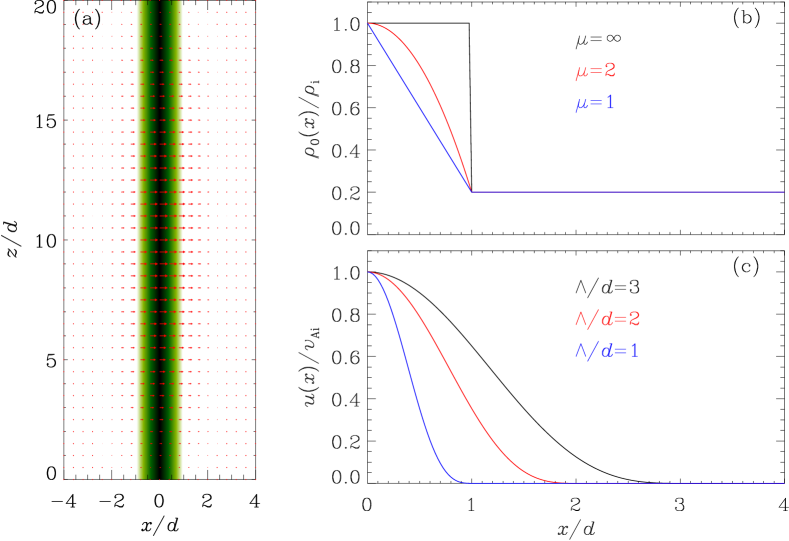
Figure 1: (a) Representation of the two-dimensional (2D) initial boundary value problem (IBVP). The $x-z$ distribution of the equilibrium density is shown by the filled contours, superimposed on which is the initial velocity field (the arrows). Axial fundamentals are ensured by the $z$-dependence of the initial perturbation. (b) Transverse profiles of the equilibrium density $\rho_{0}$ as prescribed by Eq. (10). A number of steepness parameters $\mu$ are considered as labeled, whereas the density contrast is fixed at $\rho_{\rm i}/\rho_{\rm e}=5$. (c) Transverse profiles of the initial perturbation $u(x)$ as prescribed by Eq. (13). Labeled here are a number of values of $\Lambda$, which characterizes the spatial extent of the initial exciter.

Technical details aside, linear kink motions are fully dictated by two sets of parameters. The dimensional set is taken to be $\{\rho_{\rm i},d,v_{\rm Ai}\}$, which serves merely as normalizing constants. The behavior of linear motions then hinges on the dimensionless set,

$$\{\rho_{\rm i}/\rho_{\rm e},\mu;kd=\pi d/L;\Lambda/d\}.$$ (14)

The effects of $\mu$ and $\Lambda/d$ are of primary interest, and we also adjust the density contrast $\rho_{\rm i}/\rho_{\rm e}$ when necessary. With AR loops in mind, we fix the axial wavenumber at $kd=\pi/20$. For axial fundamentals, this corresponds to an axial length $L=20d$, which lies somewhat toward the lower end of the range for AR loops typically imaged in the EUV (e.g., Aschwanden et al., 2004; Schrijver, 2007). The density contrast $\rho_{\rm i}/\rho_{\rm e}$ is taken to be in the range $[2,10]$, which is representative of AR loops as well (e.g., Aschwanden et al., 2004, and references therein).

3 EVP-based solutions: formalism

This section solves the 1D IVP formulated in Sect. 2.2 by the method of eigenfunction expansion.

3.1 EVP-based solutions for generic transverse structuring

As described in the Introduction, our approach is based on the general spectral theory of differential operators. In principle, there is no need for the initial exciter $u(x)$ to follow Eq. (13) or for the equilibrium density $\rho_{0}(x)$ to follow Eq. (10). This subsection specializes to the “inner $\mu$” prescription of $\rho_{0}(x)$ for definitiveness; nonetheless, the steepness parameter $\mu$ is allowed to be arbitrary. The corresponding formulations generalize those in Sect. 3.1 of Wang et al. (2023) where we handled $t$-dependent sausage motions in coronal slabs with step profiles.

Key to our approach is the EVP that pertains to the spatial operator $\mathcal{L}$ of the 1D IVP (see Eq. (5)). Specifically, nontrivial solutions are sought for the equation

$$\mathcal{L}\breve{v}\coloneqq-v_{\rm A}^{2}(x)\left(\dfrac{{\rm d}^{2}}{{\rm d}x^{2}}\breve{v}-k^{2}\breve{v}\right)=\omega^{2}\breve{v},$$ (15)

defined on $[0,\infty)$ and subject to the BCs (see Eq. (7))

$${\rm d}\breve{v}/{\rm d}x(x=0)=0,\quad\breve{v}(x\to\infty)<\infty.$$ (16)

Note that $k>0$ serves as an arbitrary parameter here.

One recognizes that the operator $\mathcal{L}$ is self-adjoint under the definition of the scalar product

$$\left<U|V\right>\coloneqq\int_{0}^{\infty}U^{*}(x)V(x)\rho_{0}(x){\rm d}x,$$ (17)

where the asterisk represents complex conjugate. Some properties then readily follow from general theory (see, in particular, Andries & Goossens 2007 for in-depth discussions on the self-adjoint-ness).

• All eigenvalues $\omega^{2}$ are positive, and we see the eigenfrequency $\omega$ as positive without loss of generality.

• All eigenfunctions can be made and are seen as real-valued.

• The eigenspectrum, namely the collection of $\{\omega\}$, comprises a point subspectrum and a continuum subspectrum.

• The eigenmodes in the point subspectrum are jointly characterized by some eigenfrequency $\omega_{j}$ and eigenfunction $\breve{v}_{j}$, with $j=1,2,\cdots$ being the mode label. The eigenfrequency $\omega_{j}$ is dictated by some DR, satisfying $kv_{\rm Ai}<\omega_{j}<kv_{\rm Ae}\coloneqq\omega_{\rm crit}$. The eigenfunction $\breve{v}_{j}$ is evanescent for $x>d$, making the modes “proper” in that $\breve{v}_{j}$ is square integrable (i.e., $\left<\breve{v}_{j}|\breve{v}_{j}\right>$ converges in classic sense).

• Proper eigenmodes are subject to cutoff wavenumbers $0<k_{{\rm cut},2}<k_{{\rm cut},3}<\cdots$ with the exception of the lowest mode $j=1$. By cutoff we mean that only one proper eigenmode arises when $0<k<k_{{\rm cut},2}$, while a total of $J$ proper eigenmodes are allowed when $k_{{\rm cut},J}<k<k_{{\rm cut},J+1}$ for $J\geq 2$.

• The eigenmodes in the continuum subspectrum are jointly characterized by some eigenfrequency $\omega$ and eigenfunction $\breve{v}_{\omega}$. The eigenfrequency $\omega$ continuously spans $(\omega_{\rm crit},\infty)$, meaning the irrelevance of the concept of DRs. The eigenfunction $\breve{v}_{\omega}$ is oscillatory for $x>d$, making the modes “improper” in that $\breve{v}_{\omega}$ is not square integrable (i.e., $\left<\breve{v}_{\omega}|\breve{v}_{\omega}\right>$ is not defined in classic sense).

• The eigensolutions in the proper set and the improper continuum are complete, satisfying the orthogonality condition

  $$\left<\breve{v}_{j}|\breve{v}_{j^{\prime}}\right>=\left<\breve{v}_{j}|\breve{v}_{j}\right>\delta_{j,j^{\prime}},$$ (18a)

  $$\left<\breve{v}_{j}|\breve{v}_{\omega}\right>=0,$$ (18b)

  $$\left<\breve{v}_{\omega}|\breve{v}_{\omega^{\prime}}\right>=q(\omega)\delta(\omega-\omega^{\prime}),$$ (18c)

  where $\delta_{j,j^{\prime}}$ is the Kronecker delta.

The EVP-based solution to our 1D IVP eventually writes

$$\begin{split}&\hat{v}(x,t)=\sum\limits_{j=1}^{J}c_{j}\breve{v}_{j}(x)\cos(\omega_{j}t)+\int_{kv_{\rm Ae}}^{\infty}S_{\omega}\breve{v}_{\omega}(x)\cos(\omega t){\rm d}\omega,\\ &0\leq x<\infty,\quad 0\leq t<\infty.\end{split}$$ (19)

We have made it explicit that the solution (19) is valid for arbitrary $x$ and $t$. The summation on the right-hand side (RHS) collects all (up to $J$) proper eigenmodes that may arise for a given $k$, while the integration accounts for the contribution from improper eigenmodes. The coefficients, $c_{j}$ and $S_{\omega}$, are given by

$$c_{j}=\dfrac{\left<u|\breve{v}_{j}\right>}{\left<\breve{v}_{j}|\breve{v}_{j}\right>},\quad S_{\omega}=\dfrac{\left<u|\breve{v}_{\omega}\right>}{q(\omega)}.$$ (20)

We will refer to $S_{\omega}\breve{v}_{\omega}(x)$ as some “local spectral density”.

Some general expectations can be made with Eq. (19) regarding the possible relevance of DLMs. We recall that the concept of DRs applies only to proper eigensolutions to our EVP. However, the proper and improper eigenmodes are not distinguished beforehand. Rather, this distinction arises naturally to comply with the nominal BC at infinity, where actually no restriction is imposed. We recall further that the BC at infinity in “classic BVPs” is that no ingoing waves are allowed therein. Our Appendix B collects some necessary examinations on classic BVPs, and the concept of DRs is shown to always apply. Two types of nontrivial solutions arise, with the trapped modes being identical to our proper eigenmodes. DLMs, on the other hand, are demonstrated to exist for all the examined density profiles, thereby corroborating and generalizing available findings by, say, Goedbloed et al. (2023). Now consider the oscillation frequencies of DLMs $\{\Re\Omega^{\rm DLM}\}$. Given Eq. (19), there is clearly no guarantee for $\{\Re\Omega^{\rm DLM}\}$ to stand out in a $t$-dependent solution; DLMs pertain to the classic BVP rather than our EVP. In this regard, we agree with Goedbloed et al. (2023) in saying that DLMs do not have any physical meaning per se. However, we argue that the theories on DLMs may still prove seismologically relevant if such timescales as $\{\Re\Omega^{\rm DLM}\}$ can be identified in some $t$-dependent solutions. Evidently, for DLMs to be relevant, the set $\{\Re\Omega^{\rm DLM}\}$ needs to play some special role for the frequency-dependence of $S_{\omega}$ in Eq. (19). Equally evident is that the details of the initial exciter must be crucial in determining whether this relevance materializes (see Eq. (20)).

Some further remarks are now necessary, given their immediate relevance to the “inner $\mu$” prescription in Eq. (10). We start with the following definitions,

$$k_{\rm i}^{2}\coloneqq\dfrac{\omega^{2}-k^{2}v_{\rm Ai}^{2}}{v_{\rm Ai}^{2}}=\dfrac{\omega^{2}}{v_{\rm Ai}^{2}}-k^{2},$$ (21a)

$$k_{\rm e}^{2}\coloneqq\dfrac{\omega^{2}-k^{2}v_{\rm Ae}^{2}}{v_{\rm Ae}^{2}}=\dfrac{\omega^{2}}{v_{\rm Ae}^{2}}-k^{2},$$ (21b)

$$\kappa_{\rm e}^{2}\coloneqq-k_{\rm e}^{2}=k^{2}-\dfrac{\omega^{2}}{v_{\rm Ae}^{2}},$$ (21c)

$$D\coloneqq k_{\rm i}^{2}+\kappa_{\rm e}^{2}=\dfrac{\omega^{2}}{v_{\rm Ai}^{2}}-\dfrac{\omega^{2}}{v_{\rm Ae}^{2}}.$$ (21d)

Note that $k_{\rm i}^{2}$ and $D$ are positive definite, and we see $k_{\rm i}$ as positive. Some intricacy arises for $k_{\rm e}^{2}$. We choose to work with $k_{\rm e}^{2}$ and see $k_{\rm e}$ as positive when handling improper eigenmodes ($k_{\rm e}^{2}>0$). For proper eigenmodes ($k_{\rm e}^{2}<0$), however, we always opt for $\kappa_{\rm e}^{2}$ and see $\kappa_{\rm e}$ as positive. Regardless, the following dimensionless quantities are further defined,

$$\bar{k}_{\rm i}\coloneqq k_{\rm i}d,\quad\bar{k}_{\rm e}\coloneqq k_{\rm e}d,$$ (22a)

$$\bar{\kappa}_{\rm e}\coloneqq\kappa_{\rm e}d,\quad\bar{D}\coloneqq Dd^{2},$$ (22b)

which will be used only when absolutely necessary.

We proceed to reformulate Eq. (15) into a Schrödinger form,

$$\dfrac{{\rm d}^{2}\breve{v}}{{\rm d}x^{2}}+\left[\dfrac{\omega^{2}}{v_{\rm A}^{2}(x)}-k^{2}\right]\breve{v}=0.$$ (23)

Some general results can be obtained for the uniform exterior ($v_{\rm A}(x)=v_{\rm Ae}$ for $x>d$). The external solution always writes

$$\breve{v}_{j}(x)\propto{\rm e}^{-\kappa_{\rm e}x}$$ (24)

for proper eigenmodes, and is always expressible as

$$\breve{v}_{\omega}(x)=v_{\rm Ai}\left[A_{\rm c}\cos(k_{\rm e}x)+A_{\rm s}\sin(k_{\rm e}x)\right]$$ (25)

for improper eigenmodes. Here $A_{\rm c}$ and $A_{\rm s}$ are some constants of integration. The function $q(\omega)$ in Eq. (20) evaluates to

$$q(\omega)=(\rho_{\rm e}v_{\rm Ai}^{2})\dfrac{k_{\rm e}v_{\rm Ae}^{2}}{\omega}\dfrac{\pi(A_{\rm c}^{2}+A_{\rm s}^{2})}{2}.$$ (26)

Equation (26) was first given in our previous sausage study (Wang et al., 2023, Eq. (34)), the derivation benefiting substantially from Appendix B of Oliver et al. (2015). Note that sausage and kink eigensolutions in our setup formally differ only in the interior ($x<d$). The reason for Eq. (26) to involve only the external solution is that the integral over the interior is regular and hence does not contribute (see Eqs. (17) and (18)). Note also that Eqs. (25) and (26) apply to all steepness parameters ($\mu$), whose effects show up only indirectly via $A_{\rm c}$ and $A_{\rm s}$.

Now consider the interior ($x<d$). We examine only a representative set of $\mu$, for which compact analytical solutions exist for Eq. (23). Regardless, the following aspects always hold.

• An internal eigenfunction is found by solving Eq. (23) in conjunction with the BC at $x=0$ (see Eq. (16)).

• The magnitude of an eigenfunction is irrelevant in principle. In practice, we nonetheless scale any internal improper eigenfunction $\breve{v}_{\omega}$ in such a way that it remains regular for vanishingly small $k_{\rm e}$ as happens when $\omega\to\omega_{\rm crit}=kv_{\rm Ae}$.

• The internal solution is connected to the external one by demanding the continuity of both $\breve{v}$ and ${\rm d}\breve{v}/{\rm d}x$ at $x=d$.

• We always start with improper eigenmodes. Proper eigenmodes will be described afterwards. The expression for a proper eigenfunction $\breve{v}_{j}$ is written to ensure the continuity of $\breve{v}_{j}$ itself, and the continuity of ${\rm d}\breve{v}_{j}/{\rm d}x$ then yields a DR. Expressions for $\left<\breve{v}_{j}|\breve{v}_{j}\right>$ will be offered when available. We will also analytically examine cutoff axial wavenumbers $k_{{\rm cut},j}$, but refrain from fully analyzing the DRs.

3.2 The case with $\mu=\infty$

This subsection examines the much-studied step profile ($\mu=\infty$). The internal solution to Eq. (23) is simply $\propto\cos(k_{\rm i}x)$ given that the interior is uniform. An improper eigenfunction $\breve{v}_{\omega}(x)$ writes

$$\dfrac{\breve{v}_{\omega}(x)}{v_{\rm Ai}}=\left\{\begin{array}[]{ll}\dfrac{k_{\rm e}}{k_{i}}\cos(k_{\rm i}x),&\quad 0\leq x\leq d,\\[8.5359pt] A_{\rm c}\cos(k_{\rm e}x)+A_{\rm s}\sin(k_{\rm e}x),&\quad x>d,\end{array}\right.$$ (29)

where

$$\begin{split}&A_{\rm c}=\dfrac{k_{\rm e}}{k_{\rm i}}\cos(k_{\rm i}d)\cos(k_{\rm e}d)+\sin(k_{\rm i}d)\sin(k_{\rm e}d),\\ &A_{\rm s}=\dfrac{k_{\rm e}}{k_{\rm i}}\cos(k_{\rm i}d)\sin(k_{\rm e}d)-\sin(k_{\rm i}d)\cos(k_{\rm e}d).\end{split}$$ (30)

Now consider proper eigenmodes. An eigenfunction writes

$$\dfrac{\breve{v}_{j}(x)}{v_{\rm Ai}}=\left\{\begin{array}[]{ll}{\rm e}^{-\kappa_{\rm e}d}\cos(k_{\rm i}x),&\quad 0\leq x\leq d,\\[8.5359pt] \cos(k_{\rm i}d){\rm e}^{-\kappa_{\rm e}x},&\quad x>d.\end{array}\right.$$ (33)

A rather concise expression is available for $\left<\breve{v}_{j}|\breve{v}_{j}\right>$, reading

$$\dfrac{\left<\breve{v}_{j}|\breve{v}_{j}\right>}{\rho_{\rm i}v_{\rm Ai}^{2}d}=\dfrac{{\rm e}^{-2\kappa_{\rm e}d}}{2}\left[1+\dfrac{\sin(2k_{\rm i}d)}{2k_{\rm i}d}+\dfrac{\cos^{2}(k_{\rm i}d)}{\kappa_{\rm e}d}\dfrac{\rho_{\rm e}}{\rho_{\rm i}}\right].$$ (34)

The DR governing the eigenfrequency $\omega_{j}$ writes

$$k_{\rm i}\tan(k_{\rm i}d)=\kappa_{\rm e}.$$ (35)

Cutoff wavenumbers ($k_{{\rm cut},j}$) arise when the axial phase speed $\omega/k$ approaches $v_{\rm Ae}$ in response to a varying $k$. Now that $\kappa_{\rm e}\to 0^{+}$, one recognizes from Eq. (35) that

$$k_{{\rm cut},j}d=\dfrac{(j-1)\pi}{\sqrt{\rho_{\rm i}/\rho_{\rm e}-1}},\quad(j=2,3,\cdots).$$ (36)

The expressions for both the DR (Eq. (35)) and cutoff wavenumbers (Eq. (36)) are standard textbook material (e.g., Roberts, 2019, Chapter 5), albeit largely in the context of classic BVPs.

3.3 The case with $\mu=2$

This subsection addresses the case where $\mu=2$, for which purpose the following definitions are necessary,

$$p\coloneqq\sqrt{\bar{D}}=\dfrac{\omega d}{v_{\rm Ai}}\sqrt{1-\dfrac{\rho_{\rm e}}{\rho_{\rm i}}},$$ (37a)

$$\alpha\coloneqq\dfrac{1}{4}-\dfrac{{\bar{k}_{\rm i}}^{2}}{4p}=\dfrac{1}{4}-\dfrac{(\omega d/v_{\rm Ai})^{2}-(kd)^{2}}{4p},$$ (37b)

$$X\coloneqq p(x/d)^{2}.$$ (37c)

The internal solution always writes ${\rm e}^{-X/2}M(\alpha,1/2,X)$ to respect the BC at $x=0$, with $M(\cdot,\cdot,\cdot)$ being Kummer’s $M$ function (e.g., DLMF, 2016, Chapter 13). An improper eigenfunction writes

$$\dfrac{\breve{v}_{\omega}(x)}{v_{\rm Ai}}=\left\{\begin{array}[]{ll}\bar{k}_{\rm e}{\rm e}^{-X/2}{M(\alpha,1/2,X)},&\quad 0\leq x\leq d,\\[8.5359pt] A_{\rm c}\cos(k_{\rm e}x)+A_{\rm s}\sin(k_{\rm e}x),&\quad x>d,\end{array}\right.$$ (40)

where

$$A_{\rm c}=\bar{k}_{\rm e}{\rm e}^{-X_{1}/2}M(\alpha,1/2,X_{1})\cos(k_{\rm e}d)-Q\sin(k_{\rm e}d),$$ (41a)

$$A_{\rm s}=\bar{k}_{\rm e}{\rm e}^{-X_{1}/2}M(\alpha,1/2,X_{1})\sin(k_{\rm e}d)+Q\cos(k_{\rm e}d).$$ (41b)

Furthermore, $X_{1}=p$ is the value of $X$ at $x=d$, and the symbol $Q$ is defined by

$$Q=-p{\rm e}^{-X_{1}/2}M(\alpha,1/2,X_{1})+4p\alpha{\rm e}^{-X_{1}/2}M(\alpha+1,3/2,X_{1}).$$ (42)

Here $M(\alpha+1,3/2,X_{1})$ appears because of the identify

$$\dfrac{{\rm d}}{{\rm d}\mathfrak{z}}M(a,b,\mathfrak{z})=\dfrac{a}{b}M(a+1,b+1,\mathfrak{z}).$$ (43)

Now consider proper eigenmodes. An eigenfunction writes

$$\dfrac{\breve{v}_{j}(x)}{v_{\rm Ai}}=\left\{\begin{array}[]{ll}{\rm e}^{-X/2}M(\alpha,1/2,X){\rm e}^{-\kappa_{\rm e}d},&\quad 0\leq x\leq d,\\[8.5359pt] {\rm e}^{-X_{1}/2}M(\alpha,1/2,X_{1}){\rm e}^{-\kappa_{\rm e}x},&\quad x>d.\end{array}\right.$$ (46)

A compact expression is not available for $\left<\breve{v}_{j}|\breve{v}_{j}\right>$. However, a DR may be readily derived, reading

$$-\bar{\kappa}_{\rm e}=-p+4p\alpha\dfrac{M(\alpha+1,3/2,p)}{M(\alpha,1/2,p)}.$$ (47)

The DR for trapped sausage modes in the same equilibrium was first given by Edwin & Roberts (1988). However, the DR for kink motions (Eq. (47)), is new as far as we are aware.

We proceed to derive the approximate expressions for cutoff wavenumbers $k_{{\rm cut},j}$. Interestingly, this derivation is connected to the behavior at large axial wavenumbers ($kd\to\infty$), in which case $\omega/k\to v_{\rm Ai}$. One readily deduces that $\bar{\kappa}_{\rm e}\to\infty$, $p\to\infty$, and $\bar{\kappa}_{\rm e}/p\to 1^{-}$, given their definitions (see Eqs. (21), (22), and (37)). The DR (47) then dictates that

$$\begin{split}E&\coloneqq\alpha\dfrac{M(\alpha+1,3/2,p)}{M(\alpha,1/2,p)}\\ &=\alpha\dfrac{1+\dfrac{\alpha+1}{3/2}p+\dfrac{(\alpha+1)(\alpha+2)}{(3/2)(3/2+1)2!}p^{2}+\cdots}{1+\dfrac{\alpha}{1/2}p+\dfrac{(\alpha)(\alpha+1)}{(1/2)(1/2+1)2!}p^{2}+\cdots}\\ &\to 0,\end{split}$$ (48)

where the second equal sign follows from the definition of Kummer’s $M$ function. Evidently, Eq. (48) is guaranteed provided $\alpha\to 0,-1,-2,\cdots$. One may then formally write

$$\alpha_{j}\to 1-j,\quad\mbox{for }kd\to\infty,$$ (49)

where $j=1,2,\cdots$ is recalled to be the mode label. It turns out that Eq. (49), while derived for $kd\to\infty$, holds approximately even for relatively small values of $kd$. Note that $\alpha$ evaluates to $(1-k_{\rm cut}\sqrt{\rho_{\rm i}/\rho_{\rm e}-1})/4$ at cutoffs given that $\omega/k=v_{\rm Ae}$ (see Eq. (37)). Approximating this $\alpha$ with Eq. (49) then yields that

$$k_{{\rm cut},j}d\approx\dfrac{4j-3}{\sqrt{\rho_{\rm i}/\rho_{\rm e}-1}},\quad(j=2,3,\cdots),$$ (50)

where the absence of $k_{{\rm cut},1}$ is accounted for. This approximate expression is increasingly accurate when $j$ increases, overestimating the exact value by $16.6\%$, $8.3\%$, and $5.5\%$ for $j=2,3$ and $4$, respectively.

3.4 The case with $\mu=1$

This subsection addresses the case where $\mu=1$, for which purpose the following definition is necessary

$$X\coloneqq\dfrac{-\bar{k}_{\rm i}^{2}+\bar{D}(x/d)}{\bar{D}^{2/3}}.$$ (51)

The internal solution is then a linear combination of Airy’s functions ${\rm Ai}$ and ${\rm Bi}$, reading

$$\breve{v}(x)\propto\dfrac{{\rm Ai}(X)}{{\rm Ai}^{\prime}(X_{0})}-\dfrac{{\rm Bi}(X)}{{\rm Bi}^{\prime}(X_{0})}$$ (52)

with ${\rm Ai}^{\prime}$ and ${\rm Bi}^{\prime}$ being Airy’s prime functions such that the BC at $x=0$ is respected (e.g., DLMF, 2016, Chapter 9). Furthermore,

$$X_{0}=\dfrac{-\bar{k}_{\rm i}^{2}}{\bar{D}^{2/3}}$$ (53)

evaluates $X$ at $x=0$. An improper eigenfunction writes

$$\dfrac{\breve{v}_{\omega}(x)}{v_{\rm Ai}}=\left\{\begin{array}[]{ll}\bar{k}_{\rm e}\left[\dfrac{{\rm Ai}(X)}{{\rm Ai}^{\prime}(X_{0})}-\dfrac{{\rm Bi}(X)}{{\rm Bi}^{\prime}(X_{0})}\right],&\quad 0\leq x\leq d,\\[14.22636pt] A_{\rm c}\cos(k_{\rm e}x)+A_{\rm s}\sin(k_{\rm e}x),&\quad x>d,\end{array}\right.$$ (56)

where

$$A_{\rm c}=\bar{k}_{\rm e}Y_{1}\cos(k_{\rm e}d)-\bar{D}^{1/3}Y_{1}^{\prime}\sin(k_{\rm e}d),$$ (57a)

$$A_{\rm s}=\bar{k}_{\rm e}Y_{1}\sin(k_{\rm e}d)+\bar{D}^{1/3}Y_{1}^{\prime}\cos(k_{\rm e}d).$$ (57b)

Here $Y_{1}$ and $Y_{1}^{\prime}$ are some coefficients given by

$$Y_{0}=\dfrac{{\rm Ai}(X_{0})}{{\rm Ai}^{\prime}(X_{0})}-\dfrac{{\rm Bi}(X_{0})}{{\rm Bi}^{\prime}(X_{0})},$$ (58a)

$$Y_{1}=\dfrac{{\rm Ai}(X_{1})}{{\rm Ai}^{\prime}(X_{0})}-\dfrac{{\rm Bi}(X_{1})}{{\rm Bi}^{\prime}(X_{0})},$$ (58b)

$$Y_{1}^{\prime}=\dfrac{{\rm Ai}^{\prime}(X_{1})}{{\rm Ai}^{\prime}(X_{0})}-\dfrac{{\rm Bi}^{\prime}(X_{1})}{{\rm Bi}^{\prime}(X_{0})},$$ (58c)

with $Y_{0}$ defined for immediate future use, and

$$X_{1}=\dfrac{\bar{\kappa}_{\rm e}^{2}}{\bar{D}^{2/3}}$$ (59)

being the value of $X$ evaluated at $x=d$.

Now consider proper eigenmodes. An eigenfunction writes

$$\dfrac{\breve{v}_{j}(x)}{v_{\rm Ai}}=\left\{\begin{array}[]{ll}\left[\dfrac{{\rm Ai}(X)}{{\rm Ai}^{\prime}(X_{0})}-\dfrac{{\rm Bi}(X)}{{\rm Bi}^{\prime}(X_{0})}\right]{\rm e}^{-\kappa_{\rm e}d},&\quad 0\leq x\leq d,\\[14.22636pt] \left[\dfrac{{\rm Ai}(X_{1})}{{\rm Ai}^{\prime}(X_{0})}-\dfrac{{\rm Bi}(X_{1})}{{\rm Bi}^{\prime}(X_{0})}\right]{\rm e}^{-\kappa_{\rm e}x},&\quad x>d.\end{array}\right.$$ (62)

Some algebra leads to an expression for $\left<\hat{v}_{j}|\hat{v}_{j}\right>$, which reads

$$\begin{split}\dfrac{\left<\breve{v}_{j}|\breve{v}_{j}\right>}{\rho_{\rm i}v_{\rm Ai}^{2}d}&=\dfrac{{\rm e}^{-2\bar{\kappa}_{\rm e}}}{\bar{D}^{1/3}}\left[1-\left(1-\dfrac{\rho_{\rm e}}{\rho_{\rm i}}\right)\dfrac{\bar{k}_{\rm i}^{2}}{\bar{D}}\right]\left[X_{1}Y_{1}^{2}-(Y_{1}^{\prime})^{2}-X_{0}{Y_{0}}^{2}\right]\\ &-\dfrac{{\rm e}^{-2\bar{\kappa}_{\rm e}}}{\bar{D}^{2/3}}\dfrac{1-\rho_{\rm e}/\rho_{\rm i}}{3}\left[Y_{1}^{\prime}Y_{1}-X_{1}(Y_{1}^{\prime})^{2}+X_{1}^{2}Y_{1}^{2}-X_{0}^{2}Y_{0}^{2}\right]\\ &+Y_{1}^{2}\dfrac{\rho_{\rm e}}{\rho_{\rm i}}\dfrac{{\rm e}^{-2\bar{\kappa}_{\rm e}}}{2\bar{\kappa}_{\rm e}}.\end{split}$$ (63)

When deriving Eq. (63), we have used some identities for the indefinite integrals of Airy’s functions (see Sect.9.11(iv) in DLMF, 2016). The DR for proper kink eigenmodes further writes

$$\dfrac{{\rm Ai}^{\prime}(X_{1}){\rm Bi}^{\prime}(X_{0})-{\rm Ai}^{\prime}(X_{0}){\rm Bi}^{\prime}(X_{1})}{{\rm Ai}(X_{1}){\rm Bi}^{\prime}(X_{0})-{\rm Ai}^{\prime}(X_{0}){\rm Bi}(X_{1})}=-\dfrac{\bar{\kappa}_{\rm e}}{\bar{D}^{1/3}}.$$ (64)

We note that this DR is not available in the solar literature per se, despite the well known applications of Airy’s functions in wave contexts (e.g., Snyder & Love, 1983; Li et al., 2018).

We proceed to derive the approximate expressions for cutoff wavenumbers $k_{{\rm cut},j}$, which arise when $\omega/k=v_{\rm Ae}$ and hence $\bar{\kappa}_{\rm e}=0$ (see Eqs. (21) and (22)). It follows from Eq. (59) that $X_{1}=0$, meaning that the DR (64) becomes

$$\dfrac{{\rm Ai}^{\prime}(X_{0})}{{\rm Bi}^{\prime}(X_{0})}=\dfrac{{\rm Ai}^{\prime}(0)}{{\rm Bi}^{\prime}(0)}=-\dfrac{1}{\sqrt{3}}=-\cot\dfrac{\pi}{3}.$$ (65)

Defining

$$\zeta\coloneqq\dfrac{2}{3}(-X_{0})^{3/2},$$ (66)

one finds that ${\rm Ai}^{\prime}(X_{0})/{\rm Bi}^{\prime}(X_{0})$ is well approximated by $-\cot(\zeta+\pi/4)$ (see Sect.9.7(ii) in DLMF, 2016). Note that $\bar{D}=\bar{k}_{\rm i}^{2}=k_{\rm cut}^{2}(\rho_{\rm i}/\rho_{\rm e}-1)$ at cutoffs (see Eqs. (21) and (22)). With $X_{0}$ now being $-\bar{D}^{1/3}$, Eq. (65) then leads to that

$$k_{{\rm cut},j}d\approx\dfrac{\dfrac{3}{2}\left(j-\dfrac{11}{12}\right)\pi}{\sqrt{\rho_{\rm i}/\rho_{\rm e}-1}},\quad(j=2,3,\cdots),$$ (67)

where the absence of $k_{{\rm cut},1}$ is also made explicit. This approximate expression is increasingly accurate when $j$ increases, overestimating the exact value by merely $0.7\%$ even for $j=2$.

3.5 Further remarks

This subsection presents some further remarks that help visualize the mathematical developments so far.

Figure 2: Dependency on the dimensionless axial wavenumber ($kd$) of the dimensionless axial phase speed ($\omega/kv_{\rm Ai}$) for the first several branches of proper kink eigenmodes. The density contrast is fixed at $\rho_{\rm i}/\rho_{\rm e}=5$, whereas a number of steepness parameters $\mu$ are examined in different panels. The two horizontal dashed lines represent the internal and external Alfv$\acute{\rm e}$n speeds ($v_{\rm Ai}$ and $v_{\rm Ae}$). Different branches are discriminated by the line styles as illustrated in panel a, where our convention for labeling the eigenmodes is also shown. Cutoff axial wavenumbers arise for all branches except the first one ($j=1$), their labels chosen to be consistent with our mode labeling convention. Panel a singles out the dimensionless axial wavenumber $kd=\pi/20$ to illustrate the spectrum for the EVP presented in Sect. 3.1. The continuum subspectrum is represented by the vertical arrow, the eigenfrequencies $\omega$ continuously extending from $kv_{\rm Ae}$ to infinity. Only one element is present in the point subspectrum for this chosen $kd$, and is represented by the asterisk.

Fixing the density contrast at $\rho_{\rm i}/\rho_{\rm e}=5$, Figure 2 presents how the axial phase speed ($\omega/k$) depends on the axial wavenumber ($k$) for the first several branches of proper kink eigenmodes. Different panels pertain to different values of the steepness parameter $\mu$, with the two horizontal dashed lines representing the internal and external Alfv$\acute{\rm e}$n speeds ($v_{\rm Ai}$ and $v_{\rm Ae}$). We consistently discriminate different branches by different line styles, and specifically illustrate our mode labeling convention for the step case ($\mu=\infty$, Fig. 2a). Also annotated therein are cutoff wavenumbers, which are so labeled as to be consistent with the mode labels. Note that cutoffs are absent for the first branch. Note further that the cutoff wavenumber $k_{{\rm cut},j}$ tends to increase when $\mu$ decreases for a given $\rho_{\rm i}/\rho_{\rm e}$ and a given label $j\geq 2$. In fact, $k_{{\rm cut},4}$ is so large when $\mu=2$ or $\mu=1$ that the $j=4$ branch is outside the range for plotting Figs. 2b and 2c. This behavior of cutoffs $k_{{\rm cut},j}$ can be adequately explained by their exact or approximate expressions (e.g., Eq. (36) for $\mu=\infty$).

We proceed to describe the implementation of the EVP-based solution (19). To start, we recall that the density contrast $\rho_{\rm i}/\rho_{\rm e}$ is allowed to vary between $2$ and $10$, whereas the axial wavenumber will be fixed at $kd=\pi/20$. It follows from Eq. (36) that the inequality $kd=\pi/20<k_{{\rm cut},2}$ consistently holds for the step profile ($\mu=\infty$), and therefore holds for other values of $\mu$ as well. Consequently, only one proper eigenmode is present in the point subspectrum associated with our EVP (see Sect. 3.1). Taking the step profile as example, Figure 2a then displays this proper eigenmode as the asterisk. Furthermore, the arrow is intended to represent the continuum subspectrum, with the symbol $\infty$ indicating that the eigenfrequency $\omega$ extends out to infinity. The following steps are then adopted to implement Eq. (19) for a given combination $[\rho_{\rm i}/\rho_{\rm e},kd,\Lambda/d]$.

• Given a value of $\mu$, we solve the corresponding DR for the eigenfrequency $\omega_{1}$ of the only relevant proper eigenmode, and then evaluate the associated eigenfunction $\breve{v}_{1}$. The inner products $\left<\breve{v}_{1}|\breve{v}_{1}\right>$ and $\left<u|\breve{v}_{1}\right>$ are evaluated afterwards, thereby enabling the evaluation of the coefficient $c_{1}$ (see Eq. (20)). The proper contribution is computed with the first term on the RHS of Eq. (19), taking $J=1$.

• We evaluate the eigenfunctions $\breve{v}_{\omega}$ for the continuum eigenmodes, obtaining the coefficient $A_{\rm c}$ and $A_{\rm s}$ as byproducts. The function $q(\omega)$ is then evaluated with Eq. (26), making it straightforward to evaluate the coefficient $S_{\omega}$ with Eq. (20)). The improper contribution is computed with the second term on the RHS of Eq. (19).

Despite being essentially analytical, the above steps nonetheless involve some numerical evaluations, with the integration over the continuum in Eq. (19) being an example. Convergence studies are therefore conducted to ensure that no difference can be discerned in our time-dependent solutions when, say, a different grid is employed to discretize the continuum.

4 EVP-based solutions: specific examples

4.1 General spatio-temporal patterns

Figure 3: Time-dependent solution obtained with the method of eigenfunction expansion for the combination $[\rho_{\rm i}/\rho_{\rm e}=5,\mu=\infty,kd=\pi/20,\Lambda/d=1]$. Shown is the distribution of the lateral speed $\hat{v}$ in the $x-t$ plane, with the filled contours so chosen as to better visualize the wave dynamics at short times.

This subsection presents some generic features of our time-dependent solutions. We start with a computation pertaining to $[\rho_{\rm i}/\rho_{\rm e}=5,\mu=\infty,kd=\pi/20,\Lambda/d=1]$, the lateral speed for which is displayed as a function of $x$ and $t$ in Fig. 3. One readily sees that the system evolution comprises two qualitatively different stages. The short-time response ($t\lesssim 12d/v_{\rm Ai}$ here) to the kink exciter features a series of oblique ridges in the slab exterior ($x>d$), signifying partial reflections and partial transmissions at the slab-ambient interface. By construction, these partial reflections/transmissions are associated with the improper contribution in view of the trigonometric $x$-dependence of the improper eigenfunctions ($\breve{v}_{\omega}$, Eq. (25)). The $x-t$ diagram at large times is then characterized by a series of horizontal stripes, meaning that the external perturbations eventually become laterally standing. Evidently, this standing behavior derives from the dominance of the proper contribution; see Eq. (19) and note that only one proper eigenmode is involved in the summation. The qualitative behavior in Fig. 3 is common to our $t$-dependent solutions. It is just that partial reflections/transmissions may not be readily recognizable for some combinations of $\rho_{\rm i}/\rho_{\rm e}$, $\mu$, and $\Lambda/d$.

We focus on the time sequences of the lateral speed at the slab axis, $\hat{v}(x=0,t)$, from here onward. Adopting a fixed combination $[\rho_{\rm i}/\rho_{\rm e}=5,kd=\pi/20,\Lambda/d=1]$, Figure 4 displays the $\hat{v}(x=0,t)$ profiles for different steepness parameters $\mu$ in different panels as labeled. In addition to $\hat{v}(x=0,t)$ itself (the solid curve in each panel), the contributions from proper and improper eigenmodes are further displayed by the dashed and dash-triple-dotted curves, respectively. Once again, one readily discerns the two-stage behavior. Let us first consider the proper contribution, namely a simple sinusoid with period $P_{1}=2\pi/\omega_{1}$ (see Eq. (19)). We recall that $\omega_{1}$ is only slightly smaller than $\omega_{\rm crit}=kv_{\rm Ae}$ (see Fig. 2), meaning that $P_{1}$ is only slightly longer than the axial Alfv$\acute{\rm e}$n time $2\pi/\omega_{\rm crit}=2L/v_{\rm Ae}$ ($\approx 17.9d/v_{\rm Ai}$ here) for all the examined steepness parameters. We recall further that the proper contribution is stationary in magnitude (see Eq. (19)), meaning that any overall two-stage behavior in $\hat{v}(x=0,t)$ is carried by the improper contribution. For any dash-triple-dotted curve, one then sees a transition from some rapid attenuation at short times to some later stage where the temporal attenuation is substantially slower. A comparison between different panels further indicates that this transition tends to occur later for larger $\mu$. One also sees that some short periodicities on the order of the lateral Alfv$\acute{\rm e}$n time ($d/v_{\rm Ai}$) may be present in the initial stage (e.g., Fig. 4a), and these short periodicities tend to persist longer for large $\mu$ (compare e.g., Fig. 4a with Fig. 4c). Regardless, the improper contribution at large times consistently features a longer periodicity that is only marginally below $2\pi/\omega_{\rm crit}=2L/v_{\rm Ae}$.

Figure 4: Temporal evolution of the lateral speed at the slab axis $\hat{v}(x=0,t)$. A fixed combination $[\rho_{\rm i}/\rho_{\rm e}=5,kd=\pi/20,\Lambda/d=1]$ is adopted, whereas a number of steepness parameters $\mu$ are examined in different panels as labeled. The solid curve in each panel shows the lateral speed itself. The contributions from proper and improper eigenmodes are presented by the dashed and dash-triple-dotted curves, respectively.

The temporal behavior in the improper contribution can be understood from two complementary perspectives. The first perspective, based on partial reflection/transmission, is visually more intuitive for interpreting the short periodicities ($\sim d/v_{\rm Ai}$) at early times (see also Fig. 3). Energetically, this perspective is also more intuitive in understanding the overall tendency for the improper contribution to diminish with time because this tendency can take place only via the incessant transmission of fast perturbations into the ambient fluid. Our second perspective, built directly on Eq. (19), is to attribute all the temporal features to the interference among the continuum eigenmodes. For instance, the temporal attenuation is connected to the effect whereby any adjacent monochromatic components of the continuum will become increasingly out-of-phase as time proceeds. Physically, this effect is nothing but destructive interference; the increasingly out-of-phase cosines in Eq. (19) tend to cancel out. One then expects that the low-frequency portion with $\omega\gtrsim\omega_{\rm crit}=kv_{\rm Ae}$ will gradually stand out, because it takes longer for the improper eigenmodes in this portion to get out-of-phase. This expectation is reproduced by Fig. 4 where any dash-triple-dotted curve is eventually characterized by some slow attenuation and some periodicity $\lesssim 2\pi/\omega_{\rm crit}$. One also expects that the contribution from the high-frequency portion will attenuate more rapidly, which is indeed seen at early times. That this initial stage involves high-frequency improper eigenmodes is also corroborated by the short periodicities $\sim d/v_{\rm Ai}$ therein.

Figure 5: Dependence of $c_{1}\breve{v}_{1}(x=0)$ on the density contrast $\rho_{\rm i}/\rho_{\rm e}$ for several values of $\Lambda/d$ as labeled and discriminated by linestyles. The results for the step case ($\mu=\infty$, the black curves) are compared with those for (a) $\mu=2$ (red) and (b) $\mu=1$ (blue). The axial wavenumber is fixed at $kd=\pi/20$. Note that $c_{1}\breve{v}_{1}(x=0)$ measures the magnitude of the asymptotic variation at the slab axis; see text for details.

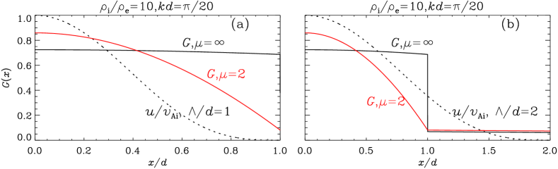
Figure 6: The function $G(x)$ plotted as solid curves over the ranges (a) $[0,d]$ and (b) $[0,2d]$ for two different steepness parameters $\mu$ as discriminated by different colors. Plotted by the dotted curves are two initial perturbations $u(x)$ with (a) $\Lambda/d=1$ and (b) $\Lambda/d=2$. A fixed combination $[\rho_{\rm i}/\rho_{\rm e}=10,kd=\pi/20]$ is employed. See text for details.

The interference perspective is applicable to broader solar contexts. We consider only those studies where the eigenfunction expansion method is adopted. We further restrict ourselves to those time intervals where some perturbation at a given position decays with time as a result of the destructive interference of continuum eigenmodes. Evidently, this interference perspective holds regardless of the origin of the continuum. We then discriminate two situations, in one of which the continuum results from the system being laterally open and in the other the continuum arises because of some continuous transverse structuring inside the domain. Our study is an example for the former. The physics is identical to what happens to wave motions in equilibrium setups with step transverse profiles for cylindrical (Oliver et al., 2014, 2015; Li et al., 2022) and slab geometries alike (Wang et al. 2023; see also Andries & Goossens 2007). What our study demonstrates is that a further physically relevant continuum does not necessarily arise when the transverse structuring is continuous. When indeed physically relevant, however, the pertinent continuum may play a vital role in explaining, say, the intricate dependence on the equilibrium quantities of damping envelopes of kink motions in coronal cylinders (Soler & Terradas 2015; see also Cally 1991). On this aspect we note that the study by Soler & Terradas (2015) focused on the resonant damping in the Alfv$\acute{\rm e}$n continuum, and hence discarded the continuum that is introduced by the system being unbounded. To our knowledge, the eigenfunction expansion method remains to be applied to the situation that physically involves continua of distinct origins.

4.2 Contribution from proper eigenmodes

This subsection focuses on the proper contribution, the purpose being to illustrate some subtleties in assessing the capabilities for the examined equilibria to confine the energy imparted by the initial exciter. An intuitive indicator will be the dimensionless axial cutoff wavenumber $k_{{\rm cut},j}d$ for any given label $j$, and we take $k_{{\rm cut},2}d$ for the ease of description. The intuition behind is that a smaller $k_{{\rm cut},2}d$ represents some stronger confinement capability. Note that $k_{{\rm cut},j}d\sqrt{\rho_{\rm i}/\rho_{\rm e}-1}$ for a given $j$ depends only on the function $f(x)$ for any equilibrium density distribution describable by Eq. (1), as explained by Li et al. (2018) even though sausage proper eigenmodes were examined therein. Specializing to our inner-$\mu$ profile (Eq. (10)), one recognizes that $k_{{\rm cut},2}d\sqrt{\rho_{\rm i}/\rho_{\rm e}-1}$ depends only on the steepness parameter $\mu$. It then follows that $k_{{\rm cut},2}d$ decreases with $\rho_{\rm i}/\rho_{\rm e}$ or $\mu$ at least for the examined steepness parameters (see Eqs. (36), (50), and (67)). This is indeed intuitive given that a slab deviates more strongly from its ambient fluid when $\rho_{\rm i}/\rho_{\rm e}$ or $\mu$ increases, and hence one expects a stronger proper contribution inside the slab. We focus on the slab axis, and take $c_{1}\breve{v}_{1}(x=0)$ to illustrate that this expectation does not necessarily hold.

Figure 5 displays $c_{1}\breve{v}_{1}(x=0)$ as a function of the density contrast $\rho_{\rm i}/\rho_{\rm e}$ for several $\Lambda/d$ as discriminated by the different linestyles. The specific values of $\Lambda/d$ are further labeled. In addition, the results for the step case ($\mu=\infty$, the black curves) are compared with those for $\mu=2$ (red, see Fig. 5a) and $\mu=1$ (blue, Fig. 5b). Examining any curve, one sees that $c_{1}\breve{v}_{1}(x=0)$ consistently increases with $\rho_{\rm i}/\rho_{\rm e}$, as expected for some stronger structuring. The $\mu$-dependence, on the other hand, is more subtle if one inspects a pair of curves with the same linestyle but different colors. The calculation for a larger $\mu$ may indeed yield a larger $c_{1}\breve{v}_{1}(x=0)$ when the initial exciter is more spatially extended (e.g., the dash-triple-dotted curves in Fig. 5a labeled $\Lambda/d=2$). However, the opposite may also take place as indicated by, say, the rightmost portions of the curves labeled $\Lambda/d=1$ in Fig. 5a.

Why does the somehow counterintuitive $\mu$-dependence occur occasionally? We address this by capitalizing on Eqs. (20) and (17) to rewrite $c_{1}\breve{v}_{1}(x=0)$ as

$$c_{1}\breve{v}_{1}(x=0)=\int\limits_{0}^{\Lambda}u(x)\dfrac{G(x)}{d}{\rm d}x,$$ (68)

where

$$G(x)\coloneqq\dfrac{[\rho_{0}(x)\breve{v}_{1}(x)]\breve{v}_{1}(x=0)}{\int_{0}^{\infty}\rho_{0}(x)\breve{v}^{2}_{1}(x){\rm d}x}d.$$ (69)

The introduction of the slab half-width $d$ into Eqs. (68) and (69) is immaterial, the purpose being simply to make $G(x)$ dimensionless. Defined this way, $G(x)$ allows the proper eigenfunction to be arbitrarily scaled. One may therefore interpret $G(x)$ in Eq.(68) as some response function of a system that is fully determined by $[\rho_{\rm i}/\rho_{\rm e},\mu,kd]$. The specific output $c_{1}\breve{v}_{1}(x=0)$ is then determined by how the input $u(x)$ is distributed over the $G(x)$ profile. We arbitrarily specialize to a combination $[\rho_{\rm i}/\rho_{\rm e}=10,kd=\pi/20]$. The response function $G(x)$ then depends only on $\mu$, and the associated profiles are plotted in Fig. 6 for two different values of $\mu$, one being $\mu=\infty$ (the black solid curves) and the other being $\mu=2$ (red). Note that Figs. 6a and 6b differ only in the range of the horizontal axis as far as the solid curves are concerned. The $u(x)$ profile is additionally plotted by the dotted curve for (a) $\Lambda/d=1$ and (b) $\Lambda/d=2$, and we note that $u(x)$ is independent of $G(x)$. A comparison between the two $G(x)$ profiles shows that they differ primarily in that $G(x)$ for $\mu=2$ exceeds its $\mu=\infty$ counterpart in the interval $x\lesssim 0.4d$. The integral in Eq. (68) then means that this portion weighs more when the initial exciter $u(x)$ is more spatially localized, making $c_{v}\breve{v}_{1}(x=0)$ larger for $\mu=2$ rather than for $\mu=\infty$. This pertains to Fig. 6a where $\Lambda/d=1$. However, the portion $x\gtrsim 0.4d$ plays a more important role when $u(x)$ is sufficiently extended, thereby explaining why $c_{v}\breve{v}_{1}(x=0)$ for $\mu=\infty$ is larger as happens when $\Lambda/d=2$ (see Fig. 6b). One may question that the subtle $\mu$-dependence in Fig. 5 holds only when $u(x)$ takes the specific form of Eq. (13), which may indeed be true. However, our point is that the interpretation of $G(x)$ as a response function provides a sufficiently general framework for understanding the system responses to different implementations of $u(x)$. Furthermore, with the subtle $\mu$-dependence we actually highlight the importance of the details of the initial exciter $u(x)$ for determining how the system responds.

4.3 Contribution from improper eigenmodes

This subsection examines the improper contribution, again specializing to the slab axis ($x=0$). Let $\hat{v}_{\rm improper}(x,t)$ denote the integral in Eq. (19). This subsection focuses specifically on the connection between the short periodicities at early times in $\hat{v}_{\rm improper}(x=0,t)$ and the pertinent DLM expectations. An examination on DLMs is therefore necessary in the framework of classic BVPs, for which we recall that the concept of DRs always applies. We present such an examination in Appendix B, where the DRs for continuous profiles are new in solar contexts. A countable infinity of modes arise for any axial wavenumber $kd$ when given a combination $[\rho_{\rm i}/\rho_{\rm e},\mu]$. Let $\Omega_{j}$ be the frequency of the $j$-th mode, and see its real part $\Re\Omega_{j}$ as positive without loss of generality. By DLMs we refer to the infinite subset of modes with the defining features that $\Re\Omega_{j}>kv_{\rm Ae}$ and $\Im\Omega_{j}<0$. In our study, all modes with $j\geq 2$ quality as DLMs for all $[\rho_{\rm i}/\rho_{\rm e},\mu]$ given the chosen $kd=\pi/20$. We nonetheless denote any such frequency as $\Omega^{\rm DLM}_{j}$ to emphasize the distinction between the oscillation frequency $\Re\Omega^{\rm DLM}_{j}$ and any (real-valued) eigenfrequency $\omega$ in our improper continuum.

Figure 7: Temporal evolution of the improper contribution as given by the integral in Eq. (19). A fixed combination $[\rho_{\rm i}/\rho_{\rm e}=5,\mu=1,kd=\pi/20]$ is adopted, whereas a number of values are examined for $\Lambda/d$ as labeled.

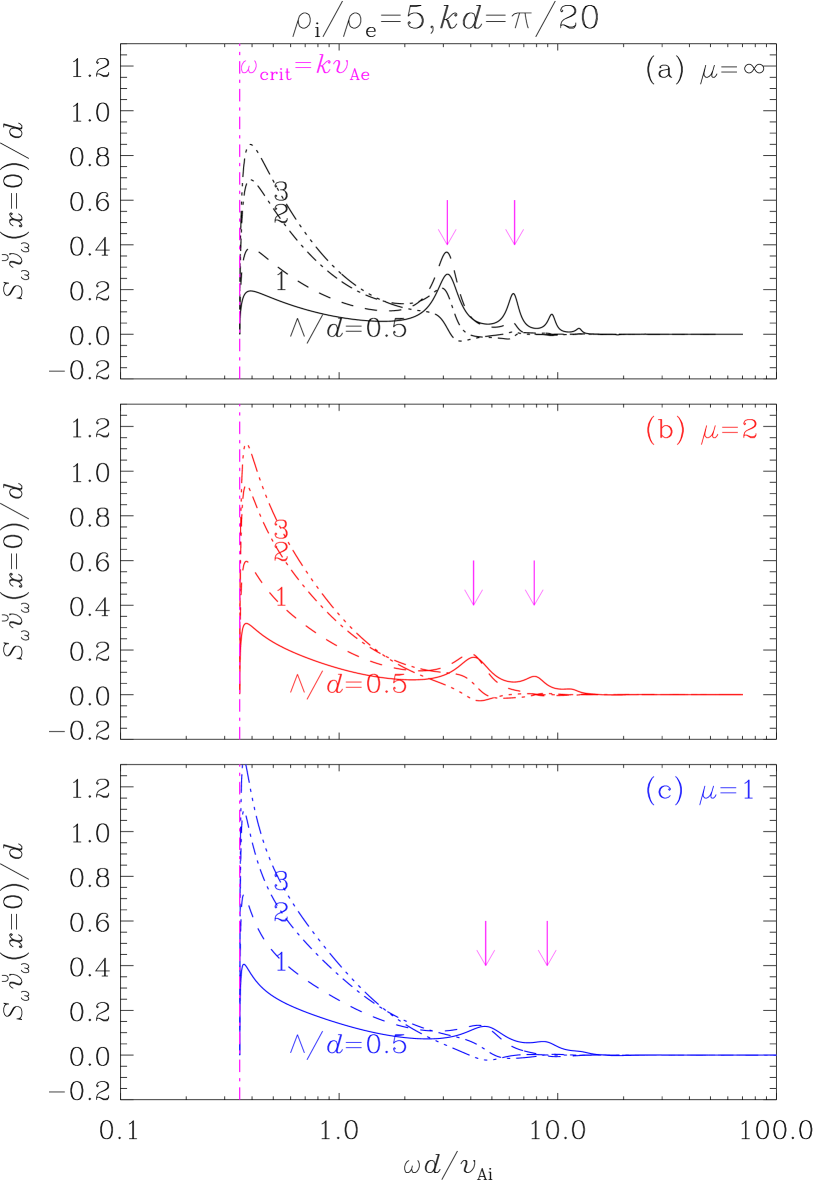
Figure 8: Frequency-dependencies of the local spectral density evaluated at the slab axis, $S_{\omega}\breve{v}_{\omega}(x=0)$. A fixed combination $[\rho_{\rm i}/\rho_{\rm e}=5,kd=\pi/20]$ is adopted, whereas a number of values are examined for the steepness parameter $\mu$ in different panels. For each $\mu$, a number of values of $\Lambda/d$ are experimented with and discriminated by the linestyles. The magenta arrows in each panel mark the oscillation frequencies of the first two discrete leaky modes ($\Re\Omega^{\rm DLM}_{2}$ and $\Re\Omega^{\rm DLM}_{3}$) computed for the same set of $[\rho_{\rm i}/\rho_{\rm e},\mu,kd]$. All vertical dash-dotted lines correspond to the critical frequency $\omega_{\rm crit}=kv_{\rm Ae}$. See text for more details.

Some general expectations follow from Eq. (19). We start by reformulating $S_{\omega}\breve{v}_{\omega}(x=0)$ as

$$S_{\omega}\breve{v}_{\omega}(x=0)=\int\limits_{0}^{\Lambda}u(x)G_{\omega}(x){\rm d}x,$$ (70)

where

$$G_{\omega}(x)\coloneqq\dfrac{\left[\rho_{0}(x)\breve{v}_{\omega}(x)\right]\breve{v}_{\omega}(x=0)}{q(\omega)},$$ (71)

and we have used Eqs. (17) and (20). Equation (70) closely resembles Eq. (68), meaning that $G_{\omega}(x)$ can also be interpreted as some response function. Note that neither $G_{\omega}(x)$ nor $\Re\Omega^{\rm DLM}_{j}$ depends on $u(x)$, and suppose for now that the combination $[\rho_{\rm i}/\rho_{\rm e},\mu,kd]$ is given. One then expects that some elements in the set $\{\Re\Omega^{\rm DLM}_{j}\}$ are bound to appear for some $u(x)$ provided that this set is special regarding the $\omega$-dependence of $G_{\omega}(x)$. It is just that whether this expectation holds depends on the details of $u(x)$, which is solely characterized by the spatial extent $\Lambda$ here.

Figure 7 takes a fixed $[\rho_{\rm i}/\rho_{\rm e}=5,\mu=1,kd=\pi/20]$ to illustrate what happens to $\hat{v}_{\rm improper}(x=0,t)$ when $\Lambda/d$ varies as labeled. Two features are evident. Firstly, some long periodicity $\sim 2\pi/kv_{\rm Ae}$ can always be identified at large times, and tends to be more prominent for larger $\Lambda$. Secondly, and more importantly, short periodicities $\sim d/v_{\rm Ai}$ do show up at early times provided that $\Lambda/d$ is sufficiently small, one example being the solid line that pertains to $\Lambda/d=0.5$. Figure 8c then address why these features arise by displaying the local spectral density $S_{\omega}\breve{v}_{\omega}(x=0)$ as a function of $\omega$, discriminating different $\Lambda/d$ by the different linestyles. The vertical dash-dotted line in magenta represents the critical frequency $\omega_{\rm crit}=kv_{\rm Ae}$. Note that $S_{\omega}\breve{v}_{\omega}(x=0)$ approaches zero when $\omega$ approaches $\omega_{\rm crit}$ from above or equivalently when $\bar{k}_{\rm e}\to 0^{+}$ (see Eq. (21)). As can be readily verified, the denominator $q(\omega)$ on the RHS of Eq. (71) scales as $\bar{k}_{\rm e}$ whereas the numerator scales as $\bar{k}_{\rm e}^{2}$ in this situation. Figure 8c then indicates that a peak always stands out in $S_{\omega}\breve{v}_{\omega}(x=0)$ (or equivalently its modulus) at some low frequency close to $\omega_{\rm crit}$ and this peak strengthens with $\Lambda/d$, thereby explaining both the persistence of the long periodicity and its $\Lambda$-dependence. On the other hand, more peaks at frequencies substantially higher than $\omega_{\rm crit}$ become increasingly prominent when $\Lambda/d$ decreases. This naturally accounts for the behavior of the short periodicities in Fig. 7. On top of that, the high-frequency peaks become increasing close to the oscillation frequencies expected for the DLMs, among which the first two ($\Re\Omega^{\rm DLM}_{2}$ and $\Re\Omega^{\rm DLM}_{3}$) are marked by the magenta arrows. Now move on to the results for (a) $\mu=\infty$ and (b) $\mu=2$. All qualitative features in Fig. 8c are seen to hold for these cases as well. Some quantitative differences arise nonetheless, one example being that the short periodicities are easier to develop for a larger $\mu$ (compare the solid curve in Fig. 8c with that in, say, Fig. 8a).

Figure 9: Dependence on $\Lambda/d$ of the frequency $\omega_{{\rm peak},2}$ where $|S_{\omega}\breve{v}_{\omega}(x=0)|$ attains the second peak. A fixed combination $[\rho_{\rm i}/\rho_{\rm e}=5,\mu=1,kd=\pi/20]$ is adopted. The hatched portion corresponds to the frequency range $[0.9,1.1]\times\Re\Omega^{\rm DLM}_{2}$. See text for details.

What makes $\Re\Omega^{\rm DLM}_{j}$ special in the improper contribution? In view of Eq. (70), the most likely reason for the systematic $\Lambda$-dependence of the high-frequency peaks is that the set $\{\Re\Omega^{\rm DLM}_{j},j\geq 2\}$ is special for the response function $G_{\omega}(x)$. However, why this happens remains puzzling because the DLMs pertain to a classic BVP, which observes a different BC from our IVP. It turns out that the function $q(\omega)$ plays a decisive role in determining the $\omega$-dependence of $G_{\omega}(x)$ (see Eq. (71)). We illustrate this point by considering the simplest case $\mu=\infty$, noting that similar arguments can be offered for other values of $\mu$. To start, we note that the inequality $|\Omega^{\rm DLM}_{j}|^{2}\gg k^{2}v_{\rm Ae}^{2}$ consistently holds in our study. When $\mu=\infty$, the DR pertinent to DLMs (Eq. (78)) then dictates that

$$\Re\Omega^{\rm DLM}_{j}d/v_{\rm Ai}\approx(j-1)\pi,\quad j=2,3,\cdots,$$ (72)

as was first shown for the limiting case $kd\to 0$ by Terradas et al. (2005). Now consider the portion of the improper continuum that satisfies $\omega^{2}\gg k^{2}v_{\rm Ae}^{2}>k^{2}v_{\rm Ai}^{2}$ and hence $k_{\rm i}^{2}\approx\omega^{2}/v_{\rm Ai}^{2},k_{\rm e}^{2}\approx\omega^{2}/v_{\rm Ae}^{2}$ (see Eq. (21)). The expressions for the coefficients $A_{\rm c}$ and $A_{\rm s}$ (see Eq. (30)) lead to that

$$A_{\rm c}^{2}+A_{\rm s}^{2}\approx\dfrac{\rho_{\rm e}}{\rho_{\rm i}}+\left(1-\dfrac{\rho_{\rm e}}{\rho_{\rm i}}\right)\sin^{2}\left(\dfrac{\omega d}{v_{\rm Ai}}\right).$$ (73)

Evidently, the values of $\Re\Omega^{\rm DLM}_{j}$ minimize $A_{\rm c}^{2}+A_{\rm s}^{2}$ and hence tend to minimize $q(\omega)$ (see Eq. (26)), meaning that these values tend to stand out as extrema in the response function $G_{\omega}(x)$ and hence in the output $S_{\omega}\breve{v}_{\omega}(x=0)$ (see Eqs. (70) and (71)). Equation (73) is reminiscent of Eq.(83) in Andries & Goossens (2007) who addressed a similar IVP with the more involved Laplace transform approach. Equation (73) bears some even closer resemblance to Eq. (39) in Wang et al. (2023) where we examined the temporal responses to sausage exciters with the same eigenfunction expansion method.

At this point, we reiterate that IVP studies in general offer a fuller picture for the wave dynamics than classic mode analyses. As concrete examples, our Figs. 7 and 8 illustrate that the DLM expectations do not necessarily materialize. That said, the concept of DLMs may still prove useful as a shortcut approach for interpreting the complicated system evolution in appropriate spatio-temporal domains. By “shortcut” we refer to the general fact that classic mode analyses are computationally much cheaper than IVP studies. Furthermore, the theoretical results for DLMs are independent from initial exciters and hence are much easier to implement than IVP studies from the seismological standpoint. It therefore should be informative to explore the requirements on the initial exciter ($\Lambda/d$ here) for the concept of DLMs to make practical sense.

Figure 9 takes $[\rho_{\rm i}/\rho_{\rm e}=5,\mu=1,kd=\pi/20]$ to illustrate how we quantify the range of $\Lambda/d$ where the concept of DLMs is useful. Basically, we focus on the $\omega$-dependence of $|S_{\omega}\breve{v}_{\omega}(x=0)|$, and systematically reduce $\Lambda/d$ to track the variation of the position of the second peak ($\omega_{{\rm peak},2}$). Note that $|S_{\omega}\breve{v}_{\omega}(x=0)|$ always features a peak at some frequency $\gtrsim\omega_{\rm crit}=kv_{\rm Ae}$, and we see this peak as the first one. Figure 9 shows a discontinuity around some sufficiently small $\Lambda/d$, which is to be denoted $(\Lambda/d)_{1}$ and reads $\sim 1.5$ in this particular case. This behavior is actually common to all of our computations, and results from our convention for numbering the peaks. Specifically, it always holds that the second peak initially moves toward higher frequencies when $\Lambda/d$ decreases toward $(\Lambda/d)_{1}$. When $\Lambda/d$ decreases further, however, an additional peak becomes identifiable at some lower frequency and therefore qualifies as our second peak. The value $\omega_{{\rm peak},2}$ then increases with decreasing $\Lambda/d$ and eventually approaches $\Re\Omega^{\rm DLM}_{2}$. Let $(\Lambda/d)_{\rm crit}$ denote the value of $\Lambda/d$ where $\omega_{{\rm peak},2}$ equals $0.9\Re\Omega^{\rm DLM}_{2}$. Equivalently, $(\Lambda/d)_{\rm crit}$ is where the $\Lambda-\omega_{{\rm peak},2}$ curve in Fig. 9 enters the hatched area, for which the lower edge is set to be $0.9\Re\Omega^{\rm DLM}_{2}$ and the upper edge is arbitrarily taken to be $1.1\Re\Omega^{\rm DLM}_{2}$. We deem the portion $\Lambda/d\leq(\Lambda/d)_{\rm crit}$ as where the concept of DLMs helps. Here the specific threshold factor $0.9$ is not that important; taking $(\Lambda/d)_{1}$ as $(\Lambda/d)_{\rm crit}$ serves our purposes equally well. One may question that the frequency range delineated by the hatched area is also crossed by the $\Lambda-\omega_{{\rm peak},2}$ curve in the portion $\Lambda/d>(\Lambda/d)_{1}$. The reason for us to discard this large-$\Lambda$ portion is that additional peaks emerge when $\Lambda/d$ decreases from $(\Lambda/d)_{1}$. Once identifiable, the positions of these peaks become almost instantly close to the expectations for additional DLMs ($\Re\Omega^{\rm DLM}_{j}$ with $j\geq 3$). This can be readily seen by comparing, say, the solid and dashed curves in Fig. 8. In other words, the occasional proximity of $\omega_{{\rm peak},2}$ to $\Re\Omega^{\rm DLM}_{2}$ for some $\Lambda/d>(\Lambda/d)_{1}$ is actually irrelevant.

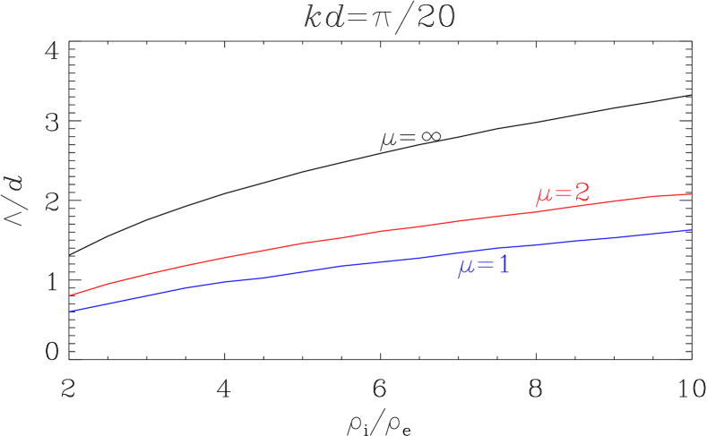
Figure 10: Dividing curves in the $\rho_{\rm i}/\rho_{\rm e}-\Lambda/d$ plane separating where the concept of discrete leaky modes helps (the portion below a curve) from where it does not (above). The axial wavenumber is fixed at $kd=\pi/20$, whereas a number of steepness parameters $\mu$ are examined as discriminated by the different colors.

Figure 10 displays $(\Lambda/d)_{\rm crit}$ as a function of the density contrast $\rho_{\rm i}/\rho_{\rm e}$ for a number of steepness parameters $\mu$ as labeled. The axial wavenumber is fixed at $kd=\pi/20$. Evidently, the curve for each $\mu$ serves as a dividing line in the $\rho_{\rm i}/\rho_{\rm e}-\Lambda/d$ plane, with the concept of DLMs being helpful only in the portion below the curve. Now see $(\Lambda/d)_{\rm crit}$ as a function of $\rho_{\rm i}/\rho_{\rm e}$ and $\mu$. Figure 10 then indicates that $(\Lambda/d)_{\rm crit}$ increases monotonically with $\rho_{\rm i}/\rho_{\rm e}$ or $\mu$ when the other parameter is fixed. Put together, this agress with the intuition that the concept of DLMs may help interpret the system evolution for a broader range of initial exciters provided that a slab makes a stronger distinction from its surroundings. However, $(\Lambda/d)_{\rm crit}$ is consistently smaller than $\sim 3.3$ for density contrasts representative of AR loops. The DLM theories therefore seem to be practically useful only for those situations where the exciters laterally span no more than several $10^{3}\leavevmode\nobreak\ {\rm km}$, given typical widths of AR loops. We argue that this spatial extent is not that small when placed in the context of, say, energy-release processes in solar flares (see e.g., the review by Shibata & Magara, 2011). In our opinion, it is more of an issue that the sort periodicities need to be resolved with a cadence higher than typically implemented for, say, EUV imagers.

5 Summary

This study was largely intended to address, in a physically transparent manner, how classic mode analyses connect to the time-dependent wave behavior in structured media. We chose to work in linear ideal MHD for simplicity, and examined axial fundamental kink motions that ensue when localized velocity perturbations are introduced to some symmetric, straight, field-aligned slab equilibria. Only two-dimensional (2D) motions were of interest, and the equiliria were taken to be structured only transversely. Continuous structuring was allowed for inside the slab, while the slab exterior was assumed to be uniform (Eqs. (1) and (10)). A 1D initial value problem (IVP) was formulated for laterally open systems, with no definitive requirement imposed at infinity. An eigenvalue problem (EVP) was constructed correspondingly, enabling the IVP to be analytically solved in terms of the complete set of eigenfunctions. This $t$-dependent solution, given by Eq. (19), allows a clear distinction between the contribution from proper eigenmodes and that due to improper eigenmodes. The wave dynamics depends on two subgroups of parameters. One subgroup characterizes the initial exciter (the dimensionless spatial extent $\Lambda/d$ here, Eq. (13)). The other subgroup characterizes the equilibria, involving the density contrast $\rho_{\rm i}/\rho_{\rm e}$, profile steepness $\mu$, and the half-width-to-length-ratio $d/L$. A systematic set of example solutions was offered for parameters representative of active region (AR) loops.

Our results are summarized as follows, where by “long” (“short”) we refer to periodicities on the order of the axial (lateral) Alfv$\acute{\rm e}$n time. Overall, all spatio-temporal patterns consistently involve the improper contribution, which nonetheless attenuates with time such that the evolution at a given location is eventually dominated by the long periodicities carried by the proper contribution. Physically, this attenuation is attributed to the destructive interference among the improper continuum. Specializing to the slab axis, we demonstrate that the proper contribution strengthens with the density contrast, but may occasionally be stronger for less steep density profiles. We find that short periodicities can be clearly identified in the improper contribution only for sufficiently localized exciters. When identifiable, these periodicities tend to agree closely with the oscillation frequencies expected for the discrete leaky modes (DLMs) in classic analyses, despite that the boundary conditions therein are different from those in our IVP. We demonstrate that the eigenfunction expansion approach allows the system response to be interpreted as the interplay between the initial exciter and some response function, the latter depending only on the equilibrium quantities (Eqs. (68) and (70)). All qualitative features can be explained as such, for proper and improper contributions alike.

Our results enable some general remarks on the seismological applicability of the extensively studied DLMs. Before anything, the examples in our Appendix B help clarify that DLMs are mathematically allowed as nontrivial solutions in classic mode analyses. Conceptually, this does not contradict the improper continuum in any example eigenspectrum in Fig. 2a; our eigensolutions observe different boundary conditions from those in classic analyses. It is therefore justifiable to say that “modes that do not exist cannot be excited” (Goedbloed et al., 2023, page 22), even though we prefer to take this as meaning the inadequacy for DLMs to account for the system evolution in the entire spatio-temporal volume. However, this inadequacy does not invalidate previous attempts that invoke the oscillation frequencies or even the exponential damping rates of DLMs to diagnose, say, the physical parameters of flaring loops in the context of flare QPPs (e.g., Kopylova et al., 2007; Nakariakov et al., 2012; Chen et al., 2015). Rather, the interference among the improper continuum eigenmodes can indeed make visible the DLM expectations. It is just that whether the DLM expectations materialize depends sensitively on the somehow intricate interplay between the initial exciter and the equilibrium setup. We take this intricacy as encouraging rather than discouraging, to illustrate which point we note that DLMs are the only modes that are accepted to yield short periodicities in classic mode analyses. Suppose that some short periodicity is observed together with some long periodicity, which is admittedly rare but not impossible (see e.g., Kolotkov et al., 2015, for a specific observation). The simultaneous use of both periodicities then helps alleviate the nonuniqueness issue for inversion problems in coronal seismology (see Arregui & Goossens, 2019, for more on this issue). Now suppose that no short periodicity can be identified in some oscillatory signal measured with adequate temporal cadence. Our Fig. 10 then allows one to deduce the minimal lateral extent of the initial exciter, thereby complementing the customary practice that focuses on diagnosing the equilibrium quantities.

Appendix A Abbreviations

This appendix lists the abbreviations in alphabetical order for the ease of reference.

AR	active region
BC	boundary condition
BVP	boundary value problem
DLM	discrete leaky mode
DR	dispersion relation
EUV	Extreme ultraviolet
EVP	eigenvalue problem
IBVP	initial boundary value problem
IC	initial condition
IVP	initial value problem
MHD	magnetohydrodynamics/magnetohydrodynamic
ODE	ordinary differential equation
PFLK	principal fast leaky kink mode
QPP	quasi-periodic pulsation
RHS	right-hand side

Appendix B Discrete leaky modes (DLMs)

This appendix provides some necessary details for the discrete leaky modes (DLMs), complementing our examination on kink motions in the main text.

Consider an equilibrium that differs from the main text only in that the domain is open in the uniform $z$-direction as well ($-\infty<z<\infty$). Restrict ourselves to strictly 2D kink perturbations. We Fourier-decompose any perturbation $f_{1}(x,z,t)$ as $\tilde{f}(x)\exp\left[-i(\Omega t-kz)\right]$, with $\tilde{f}$ being the Fourier amplitude. A “classic BVP” then results from linear, pressureless, ideal MHD. Specifically, nontrivial solutions are sought for

$$-v_{\rm A}^{2}(x)\left(\dfrac{{\rm d}^{2}}{{\rm d}x^{2}}\tilde{v}-k^{2}\tilde{v}\right)=\Omega^{2}\tilde{v},$$ (74)

defined on $[0,\infty)$ and subject to the BCs

$${\rm d}\tilde{v}/{\rm d}x(x=0)=0,$$ (75a)

$$\mbox{no ingoing waves at $x\to\infty$}.$$ (75b)

This classic BVP is almost identical to the EVP in Sect. 3.1, the only difference being the BC at infinity (Eq. (75b)).

The notations in what follows are understood to apply only in this appendix. We start by introducing the definitions,

$$\nu_{\rm i}^{2}\coloneqq\dfrac{\Omega^{2}-k^{2}v_{\rm Ai}^{2}}{v_{\rm Ai}^{2}}=\dfrac{\Omega^{2}}{v_{\rm Ai}^{2}}-k^{2},$$ (76a)

$$\nu_{\rm e}^{2}\coloneqq\dfrac{\Omega^{2}-k^{2}v_{\rm Ae}^{2}}{v_{\rm Ae}^{2}}=\dfrac{\Omega^{2}}{v_{\rm Ae}^{2}}-k^{2},$$ (76b)

$$D\coloneqq\dfrac{\Omega^{2}}{v_{\rm Ai}^{2}}-\dfrac{\Omega^{2}}{v_{\rm Ae}^{2}},$$ (76c)

together with their dimensionless counterparts

$$\bar{\nu}_{\rm i}\coloneqq\nu_{\rm i}d,\quad\bar{\nu}_{\rm e}\coloneqq\nu_{\rm e}d,\quad\bar{D}\coloneqq Dd^{2}.$$ (77)

We refer to $\Re\Omega$ as the oscillation frequency, seeing it as positive without loss of generality. We take $-\pi<\arg\bar{D}\leq\pi,-\pi/2<\arg\bar{\nu}_{\rm i},\arg\bar{\nu}_{\rm e}\leq\pi/2$. The solution in the uniform exterior always writes $\propto{\rm e}^{i\nu_{\rm e}x}$ to observe Eq. (75b). This BC turns out to be crucial in that the concept of dispersion relations (DRs) always makes sense, one shortcut derivation being to replace $\kappa_{\rm e}$ with $-i\nu_{\rm e}$ in the DRs for proper eigenmodes in the main text. The set $\{\Omega\}$, referred to as the spectrum of the classic BVP, comprises an infinity of discrete values for any axial wavenumber $kd$ given a combination $[\rho_{\rm i}/\rho_{\rm e},\mu]$. By “mode” we refer to a nontrivial solution, and we accordingly call $\Omega$ a mode frequency.

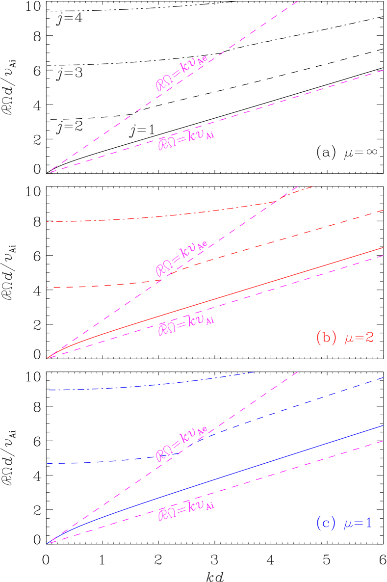
Figure 11: Dependence on the axial wavenumber ($k$) of the real part of the mode frequency ($\Re\Omega$) pertaining to the classic BVP. The density contrast is fixed at $\rho_{\rm i}/\rho_{\rm e}=5$, whereas several steepness parameters ($\mu$) are examined in different panels as labeled. The magenta dashed lines represent $\Re\Omega=kv_{\rm Ai}$ and $\Re\Omega=kv_{\rm Ae}$, the latter separating discrete leaky modes (DLMs, to its left) from trapped modes (to its right). The trapped modes are identical to the proper eigenmodes in Fig. 2; the mode labeling convention therein applies here. Mode labels with $j\geq 2$ also make sense for the DLMs, as illustrated in panel a.

We choose to write down the DRs for the BVP explicitly. Now recall that the equilibrium density is prescribed by Eqs. (1) and (10). For step profile (i.e., $\mu=\infty$), the DR writes

$$\nu_{\rm i}\tan(\nu_{\rm i}d)=-i\nu_{\rm e}.$$ (78)

For $\mu=2$, the DR reads

$$i\bar{\nu}_{\rm e}=-p+4p\alpha\dfrac{M(\alpha+1,3/2,p)}{M(\alpha,1/2,p)},$$ (79)

where $\alpha$ and $p$ are defined by

$$p\coloneqq\sqrt{\bar{D}},\quad\alpha\coloneqq\dfrac{1}{4}-\dfrac{{\bar{\nu}_{\rm i}}^{2}}{4p}.$$

The DR for $\mu=1$ writes

$$\dfrac{{\rm Ai}^{\prime}(X_{1}){\rm Bi}^{\prime}(X_{0})-{\rm Ai}^{\prime}(X_{0}){\rm Bi}^{\prime}(X_{1})}{{\rm Ai}(X_{1}){\rm Bi}^{\prime}(X_{0})-{\rm Ai}^{\prime}(X_{0}){\rm Bi}(X_{1})}=\dfrac{i\bar{\nu}_{\rm e}}{\bar{D}^{1/3}},$$ (80)

where

$$X_{0}=\dfrac{-\bar{\nu}_{\rm i}^{2}}{\bar{D}^{2/3}},\quad X_{1}=\dfrac{-\bar{\nu}_{\rm i}^{2}+\bar{D}}{\bar{D}^{2/3}}.$$

To our knowledge, Eq. (78) was first given by Terradas et al. (2005). The DRs for the two continuous density profiles, however, are not available in the literature.

Figure 11 fixes the density contrast at $\rho_{\rm i}/\rho_{\rm e}=5$ to illustrate the general mode behavior. Displayed here are the $k$-dependencies of the oscillatory frequencies ($\Re\Omega$) for a number of steepness parameters ($\mu$) in different panels as labeled. The two magenta dashed lines in each panel represent $\Re\Omega=kv_{\rm Ai}$ and $\Re\Omega=kv_{\rm Ae}$. All panels are qualitatively the same regarding the mode behavior, and hence it suffices to consider only Fig. 11a where the simplest step case ($\mu=\infty$) is examined. Modes are allowed only when $\Re\Omega>kv_{\rm Ai}$, and the spectrum at any $k$ comprises two subsets. One subset contains a finite number of real-valued $\Omega$, which consistently satisfy $\Re\Omega=\Omega<kv_{\rm Ae}$. The associated modes correspond to $\arg\bar{\nu}_{\rm e}=\pi/2$, and are the well known trapped modes (e.g., Roberts 2019, Sect. 5.5). They are identical to the proper eigenmodes examined in the main text, making it possible to invoke the concept of cutoff axial wavenumbers ($k_{{\rm cut},j}$ with $j\geq 2$). The labeling convention in Fig. 2 therefore holds here. An infinite number of complex-valued $\Omega$ are present in another subset. These are what we call DLMs, a defining feature being $\Im\Omega<0$. We label a DLM in view of its connection to the pertinent trapped branch. As noted in Terradas et al. (2005), something subtle happens when $k$ is only marginally smaller than some $k_{{\rm cut},j}$. Take $j=2$ for instance, as shown by the dashed curve in Fig. 11a. By subtle we refer to the fact that no DLM exists in a narrow interval immediately on the left of $k_{{\rm cut},2}$, meaning some broken connection between the DLM portion and the trapped portion. That said, this connection remains straightforward to identify for $j=2$, as is also the case for $j\geq 3$. Now recall that all computations in the main text pertain to a $kd$ that is consistently smaller than $k_{{\rm cut},2}$. The pertinent set of DLMs therefore starts with $j=2$.