Semiparametric inference for impulse response functions using double/debiased machine learning

Abstract

We introduce a double/debiased machine learning (DML) estimator for the impulse response function (IRF) in settings where a time series of interest is subjected to multiple discrete treatments, assigned over time, which can have a causal effect on future outcomes. The proposed estimator can rely on fully nonparametric relations between treatment and outcome variables, opening up the possibility to use flexible machine learning approaches to estimate IRFs. To this end, we extend the theory of DML from an i.i.d. to a time series setting and show that the proposed DML estimator for the IRF is consistent and asymptotically normally distributed at the parametric rate, allowing for semiparametric inference for dynamic effects in a time series setting. The properties of the estimator are validated numerically in finite samples by applying it to learn the IRF in the presence of serial dependence in both the confounder and observation innovation processes. We also illustrate the methodology empirically by applying it to the estimation of the effects of macroeconomic shocks.

JEL Classification C14  $\cdot$ C22  $\cdot$ C51  $\cdot$ C53  $\cdot$ C55

Keywords Impulse response function  $\cdot$ Double machine learning  $\cdot$ Time series  $\cdot$ Average treatment effect

1 Introduction

The estimation of the response of a time series to an external impulse is a common task in many scientific disciplines. For example, in economics, one might be interested in the reaction of the economy to a change in a central bank’s monetary policy (Angrist ., 2018). In the analysis of their trading costs, financial professionals are interested in the causal effect that their trades have on an asset’s price (Bouchaud ., 2018). In medicine, when administering a drug to a patient over time, one is interested in measuring its effect on the health of the patient (Bica ., 2020). Readers are referred to the surveys in Runge . (2023) and Raha . (2021) for more examples.

The quantity of interest in these applications is commonly referred to as the impulse response function (IRF). Ideally, the IRF measures the causal effect that an action (or “treatment”) has on the time series of interest. Recently, IRFs and ideas stemming from the causal inference framework have been related (Jordà, 2023). In particular, Rambachan  Shephard (2021) provided assumptions under which IRFs coincide with classical average treatment effects (ATE) analyzed in the potential outcomes framework of causal inference (Rubin, 1974; Robins, 1986). Given this relation between ATE and IRFs, it seams natural to adopt estimation procedures from the causal inference literature for the problem of IRF estimation. Traditionally, IRFs have primarily been estimated by modelling the entire dynamic system under consideration, e.g. using vector autoregressive processes (Sims, 1980). The seminal work of Jordà (2005) later showed how to directly estimate univariate conditional expectations using local projections (Jordà  Taylor, 2024). This approach compares the conditional expectation of an outcome variable, once conditional on a shock (treatment) and once conditional on no shock. As such, the local projection framework is directly related to the regression adjustment approach used for ATE estimation. The approach of Jordà (2005) allows for some flexibility in the estimation of the impulse response function, as it can easily incorporate polynomial and interaction terms of the regressors, or instrumental variables (Stock  Watson, 2018). More recently, Adamek . (2024) extended the local projection approach to high-dimensional settings using penalized local projections. Jordà  Taylor (2016) and Angrist . (2018) are examples of applications that use propensity score weighting for the estimation of IRFs, another common estimation approach coming from the causal inference literature, additionally accommodating asymmetric and nonlinear responses.

While estimators for IRFs have become more flexible in recent years, they still require the definition of a functional form relating treatment and outcome variable. Here, we introduce an estimator for the IRF that can rely on fully nonparametric relations between treatment and outcome variables, opening up the possibility to use flexible machine learning approaches to estimate IRFs. We consider a setting where a single time series is subjected to a discrete treatment at multiple points in time and one is interested in the average (causal) effect that these treatments have at different prediction horizons. Inspired by the approach of Chernozhukov . (2018) for the i.i.d. setting, the proposed estimator leverages the efficient influence function for the IRF in combination with cross-fitting. Instead of simply taking the difference between two estimated conditional expectations, as one would do using local projections, the efficient influence function introduces a weighted correction for the approximation errors. These weights are determined by the conditional treatment probability, or propensity score (see Equation (2)), such that a larger weight is assigned to the actual outcome when the treatment was less likely to occur. This construction makes the IRF estimation insensitive – or, formally, (Neyman-)orthogonal – to the biased estimation of the conditional expectation and treatment probability functions by machine learners. Moreover, the proposed estimator avoids over-fitting by using a cross-fitting procedure, where the time series of interest is split into two sub-sequences where the machine learning models are estimated on one sub-sequence and predictions are computed on the second sub-sequence. Then the role of the sub-sequences is reversed. These two ingredients, orthogonality and sample splitting, eliminate regularization and over-fitting bias to which machine learning algorithms are prone to, an approach coined double/debiased machine learning (Chernozhukov ., 2017). Our theoretical results show that the proposed IRF estimator is consistent and asymptotically normally distributed at the parametric rate, building the basis for semiparametric inference for dynamic effects in time series settings.

Our contribution also relates to a nascent but growing body of literature on the application of semi- and nonparametric causal inference, using machine learning, to time series problems. Lewis  Syrgkanis (2021) provide a method of estimating and conducting inference for dynamic treatment effects, based on a sequential regression peeling process, focusing on a fixed-length time series panel setup. Bica . (2020) propose an estimator for time-varying treatment effects in the presence of hidden confounders, building on a recurrent neural network. Their setting also considers a fixed-length time series observed for multiple individuals. Grecov . (2021) consider a multivariate time-series setting where some units become and remain treated at a specific point in time. The counterfactual outcomes are obtained from a global forecasting model based on a recurrent neural network. Others have employed flexible machine learning approaches for causal discovery in time series; see, among others, Yin  Barucca (2022); Bussmann . (2021); Nauta . (2019).

The paper is organized as follows. Section 2 sets up the problem. Section 3 presents the double machine learning (DML) estimator and our main theoretical results on its asymptotic properties. Proofs are relegated to Appendix A for legibility. Section 4 validates the developed theory in a simulation study. Section 5 applies the proposed estimator to policy decisions in a macrodynamic setting and Section 6 concludes.

2 Notation and identification

2.1 Notation

Let $S=\{Z_{t}^{(h)}:t\in\mathcal{T}\}$ be a stochastic process generated from a distribution $\mathcal{P}$ with $Z_{t}^{(h)}=(Y_{t+h},X_{t},D_{t})$, where $Y_{t+h}$ is a scalar real-valued random variable, $D_{t}$ a binary treatment variable, and $X_{t}\in\mathcal{X}\subseteq\mathbb{R}^{n}$ a random vector which may contain also lagged variables, including lagged values of $Y_{t}$. If not specified otherwise, $\mathcal{T}$ is a collection of ordered time indices (also referred to as the index set) with cardinality $|\mathcal{T}|=T$.

The quantity of interest is the impulse response function (IRF) at horizon $h\in\mathbb{N}_{0}$ for a binary impulse variable $D_{t}$ on the outcome variable $Y_{t+h}$ defined as (Rambachan  Shephard, 2021)

$$\theta_{0}^{(h)}=\mathbb{E}\left[\mathbb{E}[Y_{t+h}|D_{t}=1,X_{t}]-\mathbb{E}[Y_{t+h}|D_{t}=0,X_{t}]\right].$$ (1)

We focus on the case where $\theta_{0}^{(h)}$ and the conditional first moments of the outcome and treatment random variables are time-invariant.

Assumption 1.

For all $s,t\in\mathcal{T}$ and $h\in\mathbb{N}_{0}$, the following holds.

1. The impulse response function is time-invariant, i.e.

   $$\theta_{0}^{(h)}=\mathbb{E}\left[\mathbb{E}[Y_{t+h}|D_{t}=1,X_{t}]-\mathbb{E}[Y_{t+h}|D_{t}=0,X_{t}]\right]=\mathbb{E}\left[\mathbb{E}[Y_{s+h}|D_{s}=1,X_{s}]-\mathbb{E}[Y_{s+h}|D_{s}=0,X_{s}]\right]$$

2. The conditional first moments of $Y_{t+h}$ and $D_{t}$ are time-invariant, i.e.

   $$\mu_{0}(d,x,h) =\mathbb{E}[Y_{t+h}|D_{t}=d,X_{t}=x]=\mathbb{E}[Y_{s+h}|D_{s}=d,X_{s}=x],$$

   $$e_{0}(x) =\Pr(D_{t}=1|X_{t}=x)=\Pr(D_{s}=1|X_{s}=x)$$

While we present results for a binary treatment $D_{t}$, this can be generalized to multivariate discrete treatments (Angrist ., 2018), which we will also do in our empirical application. Moreover, even in settings where the treatment variable is continuous, one can obtain estimation results by discretizing the treatment of interest (see, e.g. Knaus, 2021).

We refer to $\Gamma_{0}=(\mu_{0}(d,x,h),e_{0}(x))$ as nuisance functions. As in e.g. Chernozhukov . (2018), we rely on the efficient influence function (Robins  Rotnitzky, 1995; Hahn, 1998) for estimation of the IRF, namely

$$g\left(Z_{t}^{(h)},h;\Gamma_{0}\right) =\mu_{0}(1,X_{t},h)-\mu_{0}(0,X_{t},h)$$ (2)

$$\quad+\frac{D_{t}}{e_{0}(X_{t})}(Y_{t+h}-\mu_{0}(1,X_{t},h))-\frac{1-D_{t}}{1-e_{0}(X_{t})}(Y_{t+h}-\mu_{0}(0,X_{t},h))$$

and it can be shown that

$$\theta_{0}^{(h)}=\mathbb{E}\left[g\left(Z_{t}^{(h)},h;\Gamma_{0}\right)\right].$$

Readers are referred to Kennedy (20231), Fisher  Kennedy (2021) and Tsiatis (2006) for a review of influence functions and semiparametric theory. Much of traditional estimation of IRFs relies on regression adjustment, i.e., the estimation of $\theta_{0}^{(h)}$ as the average difference between $\mu_{0}(1,X_{t},h)$ and $\mu_{0}(0,X_{t},h)$ (Cochran, 1968; Robins, 1986; Pearl, 2009; Jordà, 2005). However, regression adjustment estimators typically tend to be rather sensitive to small amounts of misspecification in the conditional expectation models. Alternatively, approaches using inverse probability weighting (Rosenbaum  Rubin, 1983; Tsiatis, 2006; Angrist ., 2018) have been devised, but are also only singly robust, thus sensitive to misspecification of the propensity score models. For the estimator presented in Section 3, we instead rely on the doubly robust influence function (2) because it has the so-called Neyman orthogonality property (Neyman, 1959, 1979; Chernozhukov ., 2017). Loosely speaking, this makes the estimator robust to small errors in the estimation of nuisance functions and thus allows the estimation of $\mu_{0}(d,x,h)$ and $e_{0}(x)$ via machine learning approaches, while still obtaining an estimator of $\theta_{0}^{(h)}$ that is consistent and asymptotically normal at the parametric rate.

In the sequel, we use standard notations $O(\cdot)$ and $o(\cdot)$ to indicate rates of convergence for sequences. In particular, if $\{x_{t}\}_{1}^{\infty}$ is any real sequence, $\{a_{t}\}_{1}^{\infty}$ a sequence of positive real numbers, and there exists a finite constant $B$ such that $|x_{t}|/a_{t}\leq B$ for all $t$, we write $x_{t}=O(a_{t})$. If $x_{t}/a_{t}$ converges to zero, we write $o(a_{t})$. We use $\left\lVert\cdot\right\rVert_{q}$ to denote the $L_{q}$-norm; e.g. we write $\left\lVert f\right\rVert_{q}=\left\lVert f(Z)\right\rVert_{q}=\left(\int|f(z)|^{q}\mathrm{d}\mathcal{P}(z)\right)^{1/q}$.

2.2 Identification

While the focus of this paper in on the estimation of the quantity introduced in Equation 1, we here briefly present assumptions under which $\theta_{0}^{(h)}$ conveys the interpretation of the average causal effect that the binary impulse variable $D_{t}$ has on the outcome variable $Y_{t+h}$. Identification is formulated within the potential outcomes framework of causal inference (Rubin, 1974; Robins, 1986). Let $Y_{t+h}(d)$ be the potential outcome, i.e., the random variable one would observe at time $t+h$ if the treatment at time $t$ would have been $D_{t}=d$. The following assumption ensures identification of the causal effect.

Assumption 2 (Angrist . (2018); Rambachan  Shephard (2021)).

For all $t\in\mathcal{T}$ and $h\in\mathbb{N}_{0}$ the following holds.

1. The potential outcomes are conditionally independent of the treatment, i.e.
   $Y_{t+h}(1),Y_{t+h}(0)\perp D_{t}|X_{t}$.

2. The observed outcome is $Y_{t+h}=D_{t}Y_{t+h}(1)+(1-D_{t})Y_{t+h}(0)$.

3. For all $x\in\mathcal{X}$ it holds that $\eta<e_{0}(x)<1-\eta$, for some $0<\eta<1$.

Assumption 2-i requires conditional independence between the treatment at time $t$ and the potential outcomes. Notably, it is not necessary for $D_{t}$ to be conditionally independent from future treatment assignments. However, in the case where $D_{t}\not\perp D_{t+1},\dots,D_{t+h}|X_{t}$, the identified effect corresponds to the effect of a treatment including potential future treatments caused by $D_{t}$ (Jordà, 2023). Assumption 2-iii imposes that at each point in time, the treatment assignment is not deterministic. In other words, there are no situations in which either $D_{t}=1$ or $D_{t}=0$ with (conditional) probability of one. For a more rigorous discussion of the identification of treatment effects with time-dependent data – and in particular for the connection between Assumption 2 and classical macroeconomic shocks – we refer to Rambachan  Shephard (2021). The following theorem finally establishes identification of the average treatment effect (ATE).

Theorem 1.

Under Assumptions 1–2 the ATE is identified as

$$\theta_{0}^{(h)} =\mathbb{E}\left[Y_{t+h}(1)-Y_{t+h}(0)\right].$$

As pointed out by Chernozhukov . (2018), the DML estimator will yield unbiased results also in a setting where the causal identification assumptions presented in this section fail to hold. In this case however, the estimated IRF has to be interpreted as a prediction difference rather than a causal effect.

3 Estimation

This section outlines the estimator for $\theta_{0}^{(h)}$ and its asymptotic properties, when the nuisance functions are estimated with flexible, nonparametric machine learning algorithms. The estimator is introduced in three steps. First, we provide results for the (hypothetical) case where the nuisance functions are known. In a second step, the nuisance functions are estimated, but two independent stochastic processes generated from the same distribution are available. Lastly, we provide results for the practically relevant case, where nuisance functions have to be estimated and only a single stochastic process is available.

3.1 An oracle estimator

In case the nuisance functions are known, we can estimate the effect of interest by simply averaging the stochastic process

$$\mathcal{G}=\left\{g\left(Z_{t}^{(h)},h;\Gamma_{0}\right):t\in\mathcal{T}\right\}$$

over the index set. We refer to this estimator as the oracle estimator for the IRF. The following assumption provides conditions under which the oracle estimator is asymptotically normally distributed.

Assumption 3.

For some $\beta>2$, the following conditions hold.

1. The stochastic process $\mathcal{G}$ is weakly stationary.

2. For the variance it holds that

   $$0<V^{(h)}_{0}=\lim_{T\to\infty}\mathrm{Var}\left[\frac{1}{\sqrt{T}}\sum_{t\in\mathcal{T}}g\left(Z_{t}^{(h)},h;\Gamma_{0}\right)\right].$$

3. The stochastic process $\mathcal{G}$ is uniformly $L_{\beta}$-bounded, i.e.

   $$\sup_{t\in\mathcal{T}}\mathbb{E}\left[\left|g\left(Z_{t}^{(h)},h;\Gamma_{0}\right)\right|^{\beta}\right]<\infty.$$

4. The stochastic process $\mathcal{G}$ is $\alpha$-mixing, with coefficients $\alpha(s)$, $s\in\mathbb{N}$, satisfying

   $$\sum_{s=1}^{\infty}\alpha(s)^{(\beta-2)/\beta}<\infty.$$

Theorem 2.

Let the oracle IRF estimator be given by

$$\tilde{\theta}^{(h)}=\frac{1}{T}\sum_{t\in\mathcal{T}}g\left(Z_{t}^{(h)},h;\Gamma_{0}\right).$$

Under Assumptions 1 and 3, we have that

$$\sqrt{T}(\tilde{\theta}^{(h)}-\theta_{0}^{(h)})\overset{d}{\to}\mathcal{N}\left(0,V^{(h)}_{0}\right),$$

with

$$V^{(h)}_{0}=\sum_{s=-\infty}^{+\infty}\mathrm{Cov}\left[g\left(Z_{t}^{(h)},h;\Gamma_{0}\right),g\left(Z_{t-s}^{(h)},h;\Gamma_{0}\right)\right].$$

Given that $g(z,h;\Gamma)$ is a measurable function as long as the nuisance functions are measurable, Assumption 3-iv is satisfied if the stochastic process $S$ is $\alpha$-mixing for some $\beta>2$ (Davidson, 2021). This is however not necessary, and $S$ can exhibit less favorable dependence structures as long as $\mathcal{G}$ adheres to Assumptions 1 and 3. Moreover, while the above assumptions are standard in the application of functional central limit theory, variations are possible that still lead to the desired asymptotics. For example, weak stationarity in Assumption 3-i can be relaxed to a constant mean, permitted that additionally $V^{(h)}_{0}<\infty$ (see e.g. the discussion in Phillips (1987)). Weak stationarity is however required in our setting in order to obtain a tractable estimator for $V^{(h)}_{0}$.

It is important to remark that the two conditions iii and iv in Assumption 3 represent an inherent trade-off. The more absolute moments of $\mathcal{G}$ are required to exist, the more dependence is acceptable in the stochastic process to still reach asymptotic normality. For the sum in Assumption 3-iv to converge, we need $\alpha(s)=O(s^{-\phi})$ for some $\phi>\phi_{0}=\beta/(\beta-2)$, i.e. the process needs to be $\alpha$-mixing of size $-\phi_{0}$. As $\beta\to\infty$ so that all moments are finite, the required mixing size $\phi_{0}\to 1$. Because the mixing coefficients also determine bounds for the (absolute) autocovariance function of the process (see Davidson (2021), Corollary 15.3), this directly implies that with all moments existing, $\mathrm{Cov}\left[g\left(Z_{t}^{(h)},h;\Gamma_{0}\right),g\left(Z_{t-s}^{(h)},h;\Gamma_{0}\right)\right]=O(s^{-1})$ for the assumptions to be satisfied.

3.2 The double machine learning estimator with two independent stochastic processes

Theorem 2 provides asymptotic results for the case where the nuisance functions $\mu_{0}(d,x,h)$ and $e_{0}(x)$ are known. We now relax this assumption and provide asymptotic results for the case where the nuisance functions are estimated. We start by presenting results where it is assumed that two independent stochastic processes generated from the same distribution $\mathcal{P}$ are available. Denote the two stochastic processes as $S_{1}=\{Z^{(h)}_{t}:t\in\mathcal{T}_{1}\}$ and $S_{2}=\{Z_{t}^{(h)}:t\in\mathcal{T}_{2}\}$ where, without loss of generality, $|\mathcal{T}_{1}|=|\mathcal{T}_{2}|=T/2$. Each stochastic processes is used once for the estimation of the nuisance functions and once for inference. The nuisance functions estimated using the stochastic process $S_{i}$ are denoted by $\hat{\mu}_{S_{i}}(d,x,h)$, $\hat{e}_{S_{i}}(x)$. The estimation procedure is outlined in Procedure 1.

Procedure 1 DML estimator for the IRF with cross-fitting on two independent stochastic processes

1. For each forecast horizon $h$ estimate $\mu_{0}(0,x,h)$, $\mu_{0}(1,x,h)$, and $e_{0}(x)$ using appropriate learning algorithms by training on $S_{1}$. Denote the estimated functions as $\hat{\Gamma}_{S_{1}}=(\hat{\mu}_{S_{1}}(d,x,h)$, $\hat{e}_{S_{1}}(x))$.

2. Compute the average of $g\left(z,h;\hat{\Gamma}_{S_{1}}\right)$ on $S_{2}$:

   $$\hat{\theta}^{(h)}_{S_{2}}=\frac{1}{|\mathcal{T}_{2}|}\sum_{t\in\mathcal{T}_{2}}g\left(Z_{t}^{(h)},h;\hat{\Gamma}_{S_{1}}\right)$$

3. Repeat steps 1. and 2. by switching the role of the stochastic processes $S_{1}$ and $S_{2}$.

4. For each forecast horizon $h$ compute the IRF estimator as:

   $$\hat{\theta}^{(h)}=\frac{|\mathcal{T}_{1}|}{T}\hat{\theta}^{(h)}_{S_{1}}+\frac{|\mathcal{T}_{2}|}{T}\hat{\theta}^{(h)}_{S_{2}}$$

For independent data, this combination of a doubly robust estimator with cross-fitting is well-known to avoid imposing complexity conditions and allows the use of flexible machine learning estimators for the nuisance functions, while still remaining amenable for semiparametric efficiency and asymptotic normality (Chernozhukov ., 2018; Robins ., 2008). The approach of randomly splitting the observations into two distinct samples as it is done for i.i.d. data, is not directly applicable in the context of time-dependent observations. In Procedure 1, we obtain independent samples for cross-fitting by assuming that two independent stochastic processes are in fact available, which is not the case in many practically relevant cases. In Section 3.3, we will relax this assumption and provide conditions under which the estimator remains consistent and asymptotically normal, even when cross-fitting is applied to a single stochastic process.

We now present asymptotic results for the DML estimator $\hat{\theta}^{(h)}$ from Procedure 1, where asymptotics are obtained for $|\mathcal{T}_{1}|,|\mathcal{T}_{2}|\to\infty$. In particular, we introduce assumptions under which $\hat{\theta}^{(h)}$ has the same asymptotic distribution as the oracle estimator $\tilde{\theta}^{(h)}$.

We impose standard assumptions on the convergence rates of the learners used in step 1. of Procedure 1. We assume that the machine learners are consistent and that the product of the approximation errors decays fast enough.

Assumption 4.

Let the realization set be $\Xi_{T}^{(h)}$, which is a shrinking neighborhood of the true nuisance functions $\Gamma_{0}=(\mu_{0}(d,x,h),e_{0}(x))$. Let $\{\Delta_{T}\}_{T\geq 1}$ and $\{\delta_{T}\}_{T\geq 1}$ be sequences of positive constants converging to zero. Define the following statistical rates:

$$r_{\mu,T} =\sup_{t\in\mathcal{T}}\sup_{\mu\in\Xi_{T}^{(h)}}\left\lVert\mu(D_{t},X_{t},h)-\mu_{0}(D_{t},X_{t},h)\right\rVert_{2}$$

$$r_{e,T} =\sup_{t\in\mathcal{T}}\sup_{e\in\Xi_{T}^{(h)}}\left\lVert e(X_{t})-e_{0}(X_{t})\right\rVert_{2}.$$

Let $C$ be a fixed strictly positive constant. For $i\in\{1,2\}$ and $h\in\mathbb{N}_{0}$, the following conditions hold.

1. The nuisance function estimators $(\hat{\mu}_{S_{i}}(0,x,h),\hat{\mu}_{S_{i}}(1,x,h),\hat{e}_{S_{i}}(x))$ belong to $\Xi_{T}^{(h)}$ with probability at least $1-\Delta_{T}$.

2. For $q>2$

   $$\sup_{t\in\mathcal{T}}\sup_{\mu\in\Xi_{T}^{(h)}} \left\lVert\mu(D_{t},X_{t},h)-\mu_{0}(D_{t},X_{t},h)\right\rVert_{q}\leq C<\infty$$

   $$\sup_{t\in\mathcal{T}}\sup_{e\in\Xi_{T}^{(h)}} \left\lVert e(X_{t})-e_{0}(X_{t})\right\rVert_{q}\leq C<\infty.$$

3. $r_{\mu,T}\leq\delta_{T}$, $r_{e,T}\leq\delta_{T}$ and $r_{\mu,T}\cdot r_{e,T}\leq T^{-1/2}\delta_{T}$.

4. $\sup_{t\in\mathcal{T}}\sup_{e\in\Xi_{T}^{(h)}}\left\lVert e(X_{t})-1/2\right\rVert_{\infty}\leq 1/2-\eta$  for $0<\eta<1$.

5. $\sup_{t}\mathbb{E}\left[\left(Y_{t+h}-\mu_{0}(d,X_{t},h)\right)^{2}|X_{t},D_{t}=d\right]\leq\epsilon^{2}_{d}<\infty$

The rates are defined in terms of uniform $L_{2}$-norms. Under the additional assumptions of strict stationarity of $S$ and measurability of the nuisance functions, the uniform norms would reduce to simple $L_{2}$-norms. Assumption 4-ii requires that, with probability approaching one, the approximation errors are uniformly $L_{q}$-bounded for $q>2$. Assumption 4-iii requires the approximation errors to converge uniformly in $L_{2}$-norm to zero and their products to converge at least at the rate $T^{1/2}$ with probability approaching one. Wong . (2020), for example, provide Lasso convergence rates for stochastic processes under the assumption of exact sparsity. For $\alpha$-mixing Gaussian processes, they find the $L_{2}$ convergence rate to be of order $O\left(A(T)\sqrt{\log{n}/T}\right)$, where $A(T)=\sum_{s=0}^{T}\alpha(s)$ and $n=\mathrm{dim}(\mathcal{X})$. Assumption 4-iii is satisfied for $A(T)=o(T^{1/4})$, imposing a restriction on how fast the dependence in the data has to decay. Assumption 4-iv ensures that the estimated propensity score is bounded away from zero and one with probability approaching one. Assumption 4-v finally requires that the conditional variance of the outcome variable is a bounded random variable.

The following theorem states that the DML estimator for the IRF is asymptotically unbiased and normally distributed. In particular, the estimator retains the parametric $\sqrt{T}$ convergence rate. The proof is relegated to Appendix A. The main idea of the proof is to show that the IRF estimator using estimated nuisance functions converges to the oracle IRF estimator $\tilde{\theta}^{(h)}$, which itself is asymptotically normally distributed as shown in Theorem 2, at rate $\sqrt{T}$.

Theorem 3.

Let $S_{1}=\left\{Z_{t}^{(h)}:t\in\mathcal{T}_{1}\right\}$ and $S_{2}=\left\{Z_{t}^{(h)}:t\in\mathcal{T}_{2}\right\}$ be two independent stochastic processes generated from the same distribution $\mathcal{P}$ such that $|\mathcal{T}_{1}|=|\mathcal{T}_{2}|=T/2$. Define the estimator as

$$\hat{\theta}^{(h)} =\frac{|\mathcal{T}_{1}|}{T}\hat{\theta}^{(h)}_{S_{1}}+\frac{|\mathcal{T}_{2}|}{T}\hat{\theta}^{(h)}_{S_{2}}$$

$$\hat{\theta}^{(h)}_{S_{1}} =\frac{1}{|\mathcal{T}_{1}|}\sum_{t\in\mathcal{T}_{1}}g\left(Z_{t}^{(h)},h;\hat{\Gamma}_{S_{2}}\right)$$

$$\hat{\theta}^{(h)}_{S_{2}} =\frac{1}{|\mathcal{T}_{2}|}\sum_{t\in\mathcal{T}_{2}}g\left(Z_{t}^{(h)},h;\hat{\Gamma}_{S_{1}}\right),$$

where the nuisance functions $\hat{\Gamma}_{S_{i}}=(\hat{\mu}_{S_{i}},\hat{e}_{S_{i}})$ are estimated using the stochastic processes $S_{i}$ respectively. Then under Assumptions 1, 3 and 4 it holds that

$$\sqrt{T}(\hat{\theta}^{(h)}-\theta_{0}^{(h)})\overset{d}{\to}\mathcal{N}\left(0,V^{(h)}_{0}\right),$$

with $V^{(h)}_{0}$ as in Theorem 2.

3.3 The double machine learning estimator with one stochastic process

In practice, two independent stochastic processes generated from the same distribution are often not available. Instead, a sample from a single stochastic process $S$ is observed. Inspired by the approaches used for cross-validating models with dependent data (Bergmeir  Benítez, 2012; Racine, 2000), we split the single stochastic process into two sub-sequences, removing a block of $k_{T}$ coordinates between them. These sub-sequences are then used in place of the samples $S_{1}$ and $S_{2}$ in Procedure 1. The approach is described in Procedure 2.

Procedure 2 DML estimator for the IRF with cross-fitting on a single stochastic processes

1. Split the stochastic process $S=\{Z^{(h)}_{t}:t\in\mathcal{T}\}$ into two sub-processes $S_{1}=\{Z^{(h)}_{t}:t\in\mathcal{T}_{1}\}$ and $S^{(h)}_{2}=\{Z_{t}:t\in\mathcal{T}_{2}\}$ such that $\min(\mathcal{T}_{2})-\max(\mathcal{T}_{1})=k_{T}\geq 0$.

2. For each forecast horizon $h$ estimate $\mu_{0}(0,x,h)$, $\mu_{0}(1,x,h)$, and $e_{0}(x)$ using an appropriate learning algorithm by training on $S_{1}$. Denote the estimated functions as $\hat{\Gamma}_{S_{1}}=(\hat{\mu}_{S_{1}},\hat{e}_{S_{1}})$.

3. Compute the average of $g\left(z,h;\hat{\Gamma}_{S_{1}}\right)$ on $S_{2}$:

   $$\hat{\theta}^{(h)}_{S_{2}}=\frac{1}{|\mathcal{T}_{2}|}\sum_{t\in\mathcal{T}_{2}}g\left(Z_{t}^{(h)},h;\hat{\Gamma}_{S_{1}}\right)$$

4. Repeat steps 2. and 3. by switching the role of the stochastic processes $S_{1}$ and $S_{2}$.

5. For each forecast horizon $h$ compute the IRF estimator as:

   $$\hat{\theta}^{(h)}=\frac{|\mathcal{T}_{1}|}{T-k_{T}}\hat{\theta}^{(h)}_{S_{1}}+\frac{|\mathcal{T}_{2}|}{T-k_{T}}\hat{\theta}^{(h)}_{S_{2}}$$

The asymptotic results for the estimator described in Procedure 2 require some additional assumptions.

Assumption 5.

For $d\in\{0,1\}$, $h\in\mathbb{N}_{0}$ and some scalar constant $p\geq 1$ the following conditions hold.

1. For $T\to\infty$ it holds that $T^{-1}k_{T}=o(1)$.

2. The nuisance functions $\mu_{0}(d,x,h)$, $e_{0}(x)$ and the functions $\mu(d,x,h),e(x)\in\Xi_{T}^{(h)}$ are measurable.

3. For for $r>p$ and $1/r=1/r^{\prime}+1/r^{\prime\prime}$

   $$\sup_{t\in\mathcal{T}}\,\lVert\sup_{\mu\in\Xi_{T}^{(h)}}(\mu(d,X_{t},h)-\mu_{0}(d,X_{t},h))\lVert_{2r^{\prime}}<\infty\qquad\text{and}\qquad\sup_{t\in\mathcal{T}}\left\lVert e_{0}(X_{t})-D_{t}\right\rVert_{2r^{\prime\prime}}<\infty$$

   .

4. For $q>p$ and $1/q=1/q^{\prime}+1/q^{\prime\prime}$

   $$\sup_{t\in\mathcal{T}}\,\lVert\sup_{e\in\Xi_{T}^{(h)}}(e(X_{t})-e_{0}(X_{t}))\lVert_{2q^{\prime}}<\infty\qquad\text{and}\qquad\sup_{t\in\mathcal{T}}\left\lVert Y_{t}-\mu_{0}(D_{t},X_{t},h)\right\rVert_{2q^{\prime\prime}}<\infty$$

   .

5. The stochastic process $S=\{Z_{t}^{(h)}:t\in\mathcal{T}\}$ is $\alpha$-mixing with coefficients $\alpha(s)$, satisfying for $T\to\infty$ that

   $$\alpha\left(k_{T}\right)^{\psi}=o(T^{-1}),$$

   where $\psi=1/p-1/\min(r,q)$.

Assumption 5 imposes restrictions on the dependence structure in the stochastic process $S$. As we can no longer rely on the independence between $S_{1}$ and $S_{2}$, we require the dependence of the stochastic process to decay fast enough. Intuitively, after removing $k_{T}$ coordinates between the samples, $S_{1}$ and $S_{2}$ should become (asymptotically) independent. The choice of $k_{T}$ hereby represents a trade-off. The larger $k_{T}$, the smaller is the effective sample size. Indeed, Assumption 5-i requires $k_{T}$ to increase less rapidly than the sample size. However, $k_{T}$ needs to be large enough to satisfy Assumption 5-v. The stronger the dependence in the stochastic process $S$, the larger $k_{T}$ needs to be, in turn reducing the effective sample size. For the sake of exposition, assume that $k_{T}=O(T^{\vartheta})$ and let us look at different exemplary assumptions on the dependence structure of the residuals.

$\alpha$-mixing process: If the stochastic process $S$ is $\alpha$-mixing of size $-\phi_{0}$, i.e. $\alpha(s)=O(s^{-\phi})$ for some $\phi>\phi_{0}$, then Assumption 5-v is satisfied for $\vartheta>(\phi\psi)^{-1}$ and $0<\psi<1$. Put differently, the slower the decay in the dependence (smaller $\phi$), the larger $\vartheta$ and thus $k_{T}$ has to be.

Persistent process: For stochastic processes $S$ with very slowly decaying dependence of the form $\alpha(s)=O(s^{2d-1})$ with $0<d<1/2$, we have additionally that $0<\phi<1$ and as a consequence Assumption 5-v is indeed never satisfied.

Weakly dependent processes: If the stochastic process $S$ has mixing coefficients $\alpha(s)=O(\rho^{s})$ for $0<\rho<1$, then Assumption 5-v is already satisfied with $\vartheta>0$.

Independent process: In this case, i.e. when it is assumed that the stochastic process $S$ is a collection of independent random variables, then $\alpha(s)=0$ for all $s$ and Assumption 5-v is already satisfied for $k_{T}=0$.

These examples intuit two things that are required for our theory to hold in practice. First, if only one stochastic process $S$ is available for estimation, enough coordinates must be removed when splitting, so that no influence of past coordinates exists in coordinates of a subsequent split. Second, the stochastic processes $S$ itself has to exhibit fast enough decaying temporal dependence. If this is not the case, suitable transformations of the original process need to be found to achieve this. Lastly, the boundedness conditions in the above assumptions also represent a trade-off. The more moments of the residual and forecast error sequences are finite (larger $r$ and $q$), the less stringent are the conditions on the dependence decay, and vice versa. In general, with only one stochastic process, the conditions on the approximation errors are more restrictive than those imposed in Assumption 4-ii.

The following theorem finally establishes asymptotic properties for the case when nuisance functions are estimated based on a single stochastic process.

Theorem 4.

Given the stochastic process $S=\{Z_{t}^{(h)}:t\in\mathcal{T}\}$, define two sub-sequences $S_{1}=\left\{Z_{t}^{(h)}:t\in\mathcal{T}_{1}\right\}$ and $S_{2}=\left\{Z_{t}^{(h)}:t\in\mathcal{T}_{2}\right\}$ such that for the index sets it holds that

$$\mathcal{T}_{1}\cup\mathcal{T}_{2}\subseteq\mathcal{T}$$

$$\min(\mathcal{T}_{2})-\max(\mathcal{T}_{1})=k_{T}\geq 0$$

$$|\mathcal{T}_{1}|=|\mathcal{T}_{2}|=\frac{T-k_{T}}{2}.$$

Define the estimator as

$$\hat{\theta}^{(h)} =\frac{|\mathcal{T}_{1}|}{T-k_{T}}\hat{\theta}^{(h)}_{S_{1}}+\frac{|\mathcal{T}_{2}|}{T-k_{T}}\hat{\theta}^{(h)}_{S_{2}}$$

$$\hat{\theta}^{(h)}_{S_{1}} =\frac{1}{|\mathcal{T}_{1}|}\sum_{t\in\mathcal{T}_{1}}g\left(Z_{t}^{(h)},h;\hat{\Gamma}_{S_{2}}\right)$$

$$\hat{\theta}^{(h)}_{S_{2}} =\frac{1}{|\mathcal{T}_{2}|}\sum_{t\in\mathcal{T}_{2}}g\left(Z_{t}^{(h)},h;\hat{\Gamma}_{S_{1}}\right),$$

where the nuisance functions $\hat{\Gamma}_{S_{i}}=(\hat{\mu}_{S_{i}},\hat{e}_{S_{i}})$ are estimated using the sub-sequence $S_{i}$ respectively. Then under Assumptions 1, 3, 4 and 5 it holds that

$$\sqrt{T-k_{T}}(\hat{\theta}^{(h)}-\theta_{0}^{(h)})\overset{d}{\to}\mathcal{N}\left(0,V^{(h)}_{0}\right),$$

with $V^{(h)}_{0}$ as in Theorem 2.

3.3.1 Variance estimation and inference

The variance $V^{(h)}_{0}$ can be estimated using standard long-run variance estimators for time series, such as the one proposed by Newey  West (1987).

Assumption 6.

The following conditions hold.

1. There are some fixed finite constants $C$ and $r>4$ such that

   $$\sup_{t\in\mathcal{T}}\mathbb{E}\left[\left|g\left(Z_{t}^{(h)},h;\Gamma_{0}\right)\right|^{r}\right]<C.$$

2. There exists a measurable function $m(z)$ such that $\sup_{\Gamma\in\Xi_{T}}|g(z,h;\Gamma)|<m(z)$, where for some finite constant $D$, $\sup_{t\in\mathcal{T}}\mathbb{E}[m(Z_{t})^{2}]<D$.

3. The bandwidth $m_{T}$ is a function of the sample size such that $\lim_{T\to\infty}m_{T}=\infty$ and for $T\to\infty$ it holds that $T^{-1/4}m_{T}=o(1)$.

4. For $q>2$ and some fixed strictly positive and finite constant $C$ we have $\sup_{t\in\mathcal{T}}\left\lVert Y_{t}\right\rVert_{q}\leq C$.

5. $r_{\mu,T}\leq\delta_{T}T^{-1/4}$ and $r_{e,T}\leq\delta_{T}T^{-1/4}$.

The following theorem establishes consistency of a variance estimator resulting from averaging Newey  West (1987) type estimators per sub-sequence.

Theorem 5.

Given the stochastic process $S=\{Z_{t}^{(h)}:t\in\mathcal{T}\}$, define two sub-sequences $S_{1}$ and $S_{2}$ as in Theorem 4. Furthermore, define

$$v^{(h)}_{t}=g\left(Z^{(h)}_{t},h;\Gamma_{0}\right)-\theta^{(h)}_{0}$$

and the corresponding estimated quantity as

$$\hat{v}^{(h)}_{S_{i},t}=g\left(Z^{(h)}_{t},h;\hat{\Gamma}_{S_{i}}\right)-\hat{\theta}^{(h)},$$

where the nuisance functions $\hat{\Gamma}_{S_{i}}=(\hat{\mu}_{S_{i}},\hat{e}_{S_{i}})$ are estimated on the sub-sequence $S_{i}$ and $\hat{\theta}^{(h)}$ is defined in Theorem 4. Let $w(s,m_{T})=1-s/(m_{T}+1)$, where $m_{T}$ is a bandwidth parameter and define the index set

$$\mathcal{T}_{i,s}=\{t\in\mathcal{T}_{i}\,|\,t-s\geq\min(\mathcal{T}_{i})\}.$$

Moreover, define the following Newey  West (1987) type variance estimators for each sub-sequence as

$$\widehat{V}^{(h)}_{S_{1}} =\frac{1}{|\mathcal{T}_{1}|}\left(\sum_{t\in\mathcal{T}_{1}}(\hat{v}^{(h)}_{S_{2},t})^{2}+2\sum_{s=1}^{m_{T}}w(s,m_{T})\sum_{t\in\mathcal{T}_{1,s}}\hat{v}^{(h)}_{S_{2},t}\hat{v}^{(h)}_{S_{2},t-s}\right)$$

$$\widehat{V}^{(h)}_{S_{2}} =\frac{1}{|\mathcal{T}_{2}|}\left(\sum_{t\in\mathcal{T}_{2}}(\hat{v}^{(h)}_{S_{1},t})^{2}+2\sum_{s=1}^{m_{T}}w(s,m_{T})\sum_{t\in\mathcal{T}_{2,s}}\hat{v}^{(h)}_{S_{1},t}\hat{v}^{(h)}_{S_{1},t-s}\right).$$

The variance estimator is finally defined as

$$\widehat{V}^{(h)}=\frac{|\mathcal{T}_{1}|}{T-k_{T}}\widehat{V}^{(h)}_{S_{1}}+\frac{|\mathcal{T}_{2}|}{T-k_{T}}\widehat{V}^{(h)}_{S_{2}}.$$

Then under Assumptions 1, 3, 4, 5 and 6 as $T\to\infty$ it holds that

$$|\widehat{V}^{(h)}-V^{(h)}_{0}|\overset{p}{\to}0$$

with $V^{(h)}_{0}$ as in Theorem 2.

Note that while Theorem 5 is formulated in terms of a specific weight function $w(s,m)$, as in Newey  West (1987), the variance estimator is consistent for any weight function additionally satisfying for each $s$ that $\lim_{m(T)\to\infty}w(s,m_{T})=1$ and $|w(s,m_{T})|<\infty$. Using the estimators in Theorems 4 and 5, inference can be conducted by constructing level-$\alpha$ confidence bounds for $\theta_{0}^{(h)}$ as

$$\theta^{(h)}_{0}\in\left(\hat{\theta}^{(h)}\pm\frac{1}{\sqrt{T-k_{T}}}\Phi^{-1}\left(1-\frac{\alpha}{2}\right)\sqrt{\widehat{V}^{(h)}}\right),$$ (3)

where $\Phi^{-1}(\cdot)$ represents the inverse cumulative distribution function of the standard normal distribution.

3.4 Considerations on the practical implementation of the estimator

Here, we gather some recommendations on the implementation of the DML estimator for time series problems in practice.

3.4.1 Cross-fitting

As in the case of cross-fitting for i.i.d. data, Procedure 2 can be extended to a setting with $K>2$ sub-sequences of the stochastic process, where $K-1$ sub-processes are used in step 2. and the remaining one in step 3. Steps 2. and 3. are then repeated $K-1$ times. In order to use as many observations as possible, we recommend dividing the observed sample into $K$ sub-sequences and drop $k_{T}$ observations only at the boundary between the $K-1$ sub-sequences used for the estimation of the nuisance functions and the sub-sequence used for computing predictions. This is illustrated in Figure 1 for $K=4$, i.e. the time series is divided into four sub-sequences. The nuisance functions are estimated on sub-sequences $S_{1}$, $S_{2}$ and $S_{4}$. Sub-sequence $S_{3}$ is used to compute $\hat{\theta}^{(h)}_{S_{3}}$, where $k_{T}$ coordinates are dropped at the boundaries of $S_{3}$. This procedure is repeated such that each sub-sequence is used once to compute predictions.

For small samples, we recommend setting $K$ to a rather large value (e.g. $K=10$). This increases the number of observations available to estimate the nuisance functions. Furthermore, while we presented our theoretical results by removing $k_{T}/2$ observations from both the estimation and the evaluation sample, asymptotically it is irrelevant whether the $k_{T}$ observations are removed only from the estimation/evaluation sample, or in parts from both samples. Thus, in small samples, we advise to remove the $k_{T}$ observations from the data used to estimate the machine learners. This ensures that all observations are used in the computation of the IRF (step 3. of Procedure 2).

Note that the choice of $k_{T}$ is also directly affected by the definition of the outcome variable. In cases where the effect on the outcome variable $h$ periods after the treatment is of interest, $k_{T}$ has to be chosen such that the two samples are not overlapping, i.e. $k_{T}\geq h$. Similarly, $k_{T}$ has to take into account possible lagged values in $X_{t}$.

Figure 1: Example of Procedure 2 with $K=4$. The nuisance functions are estimated using appropriate machine learners on sub-sequences $S_{1}$, $S_{2}$ and $S_{4}$. Sub-sequence $S_{3}$ is used to compute $\hat{\theta}^{(h)}_{S_{3}}$, where $k_{T}$ coordinates are dropped at the boundaries of $S_{3}$. This procedure is repeated such that each sub-sequence is used once to compute predictions.

3.4.2 Estimators for the nuisance functions

As in the i.i.d. setting, our theory requires the estimators for the nuisance functions to be consistent with fast enough convergence rates (Chernozhukov ., 2018). Following Theorems 3 and 4, this needs to extend now to estimation on time-dependent observations. Consistency and convergence rates on $\alpha$-mixing sequences are derived for Lasso in Wong . (2020), for random forests in Goehry, Benjamin (2020), for boosting algorithms in Lozano . (2014), for support vector machines in Steinwart . (2009), for kernel and nearest-neighbour regressions in Irle (1997) and for spline and wavelet series regression estimators in X. Chen  Christensen (2015). Consistency of deep feed-forward neural networks with ReLU activation functions on exponentially $\alpha$-mixing processes was recently shown in Ma  Safikhani (2022). Our numerical experiments suggest that, as in the i.i.d. case (Bach ., 2024), properly tuning hyperparameters of the chosen estimators plays an important role in the application of double machine learning also for time series data. We recommend to train and tune multiple different estimators and select the best in terms of the relevant loss function for the problem at hand (e.g. predictive mean squared error).

3.4.3 Modelling multiple forecast horizons

Our theory is agnostic to how the nuisance functions for different forecast horizons $h$ are modelled. In analogy to classical impulse response function estimation using local projections, each forecast horizon (and nuisance function) can be estimated separately, and potentially with different learning algorithms. Depending on the application, it is however also possible to estimate $\mu_{0}(d,x,h)$ with one model for all $h$, e.g. using sequence-to-sequence approaches (Mariet  Kuznetsov, 2019). Applying approaches from multitask learning (Caruana, 1997), it is finally also possible to estimate $\mu_{0}(d,x,h)$ and $e_{0}(x)$ in one model if both problems can be learned using a shared representation. This approach has been explored by e.g. Shi . (2019) in the context of i.i.d. data.

4 Simulation experiments

To validate our theoretical results from the previous sections in finite samples, we conduct simulation experiments. We compare the DML estimator from Procedures 1 and 2 to a regression adjustment estimator that estimates the nuisance functions $\mu_{0}(1,x,h)$ and $\mu_{0}(0,x,h)$ separately and takes their difference (a T-learner in the terminology of Künzel . (2019)). To assess the effect of cross-fitting, we apply the regression adjustment estimator once with (RA^c) and once without cross-fitting (RA). In addition, we estimate the impulse response functions using standard local projections (LP) (Jordà, 2005). Results are presented throughout using random forests (Breiman, 2001) as machine learning estimators for the nuisance functions. In the Appendix, Table D2, we also include results using a gradient boosting algorithm estimator (T. Chen  Guestrin, 2016), supporting the validity of our asymptotic theory for alternative machine learning estimators. More details on the hyperparameter tuning schemes for both considered estimators are also given in Appendix B.

In all simulations, we generate data according to the following data generating process (DGP), which is a modification of the setup in Nie  Wager (2020). For some noise level $\sigma_{\epsilon}$, a propensity score $e_{0}(X_{t})$, a baseline effect $b(X_{t})$ and a (conditional) treatment effect function $\tau(X_{t})$, the outcome process is defined as

$$Y_{t} =b(X_{t})+\left(D_{t}-0.5\right)\tau(X_{t})+\gamma Y_{t-1}+\epsilon_{t},$$ (4)

where the innovations $\epsilon_{t}$ are generated from an ARFIMA($a$,$d_{y}$,$b$) process

$$\phi(L)(1-L)^{d_{y}}\epsilon_{t}=\beta(L)\zeta_{t},$$

where $L$ is the lag operator such that $L\epsilon_{t}=\epsilon_{t-1}$. The scalar $d_{y}\in(-0.5,0.5)$ denotes the fractional differencing parameter, $\phi(L)=1-\phi_{1}L-\phi_{2}L^{2}-...-\phi_{a}L^{a}$, $\beta(L)=1-\beta_{1}L-\beta_{2}L^{2}-...\beta_{b}L^{b}$ and $\zeta_{t}\sim\mathcal{N}(0,\sigma_{\zeta}^{2})$, where $\sigma_{\zeta}^{2}$ is chosen such that $\mathbb{E}[\epsilon^{2}_{t}]=\sigma_{\epsilon}^{2}$. We will fix $\beta_{i}=1~{}\forall i$, $a=0$ for the experiments and set

$$D_{t}|X_{t} \sim\text{Ber}\left(e_{0}(X_{t})\right)$$ (5)

$$e_{0}(X_{t}) =\left(1+e^{-X_{1,t}}+e^{-X_{2,t}}\right)^{-1}$$

$$b(X_{t}) =0.5\left((X_{1,t}+X_{2,t}+X_{3,t})^{+}+(X_{4,t}+X_{5,t})^{+}\right)$$

$$\tau(X_{t}) =(X_{1,t}+X_{2,t}+X_{3,t})^{+}-(X_{4,t}+X_{5,t})^{+}$$

where $(x)^{+}=\max(0,x)$.

We use the ARFIMA innovations for $Y_{t}$ in order to explore two settings. A first one where the assumptions of our theory are satisfied and a second one where Assumption 3-iv is violated. In particular, when $d_{y}=0$, then $Y_{t}$ reduces to a standard ARMA process with Gaussian innovations and is $\alpha$-mixing (Mokkadem, 1988) (and thus so is $\mathcal{G}$), but when $d_{y}\neq 0$, then $\epsilon_{t}$ has hyperbolically decaying autocovariance and is not $\alpha$-mixing (Helson  Sarason, 1967).

The confounder process $\{X_{t}:t=1,\dots,T\}$ is finally modelled as a $n$-dimensional, zero mean VARMA($p$,$q$) process

$$X_{t}=\sum_{i=1}^{p}A_{i}X_{t-i}+\sum_{j=1}^{q}M_{j}u_{t-j}+u_{t},$$ (6)

where, as usual, $u_{t}$ is a zero mean white noise random variable with nonsingular covariance matrix, which we parametrize as $\Sigma_{u}=\sigma^{2}_{u}I_{n}$ using some scalar $\sigma_{u}$ and the $n$-dimensional identity matrix $I_{n}$. The coefficient matrices are defined as $A_{i}=\alpha_{A}^{i-1}\Gamma^{A}$ and $M_{j}=\alpha_{M}^{j-1}\Gamma^{M}$, where $\alpha_{A},\alpha_{M}$ are some scalars, $\Gamma^{A}$ (and $\Gamma^{M}$ correspondingly) is a tapered Toeplitz matrix with $\Gamma^{A}_{i,j}=\rho_{A}^{|i-j|+1}$ and $\Gamma^{A}_{i,j}=0$ for $|i-j|\geq n/2$. We finally scale the process $X_{t}$ so that the confounders have unit variance. The parameters are set to $\gamma=0.6$, $p=2$, $q=1$, $\sigma^{2}_{u}=1.0$, $\alpha_{A}=0.3$, $\alpha_{M}=0.3$, $\rho_{A}=0.35$, $\rho_{M}=0.7$. For the baseline simulation we set $n=12$, $\sigma_{\epsilon}=1$ and generate the innovations of the outcome process from a MA(5) process ($d_{y}=0$ and $b=5$). Results for a larger set of possible confounders ($n=20$) or a lower signal-to-noise ratio ($\sigma_{\epsilon}=3$) are relegated to Appendix D. The full simulation procedure is described in Procedure 3.

Procedure 3 Simulation

1. For each evaluated forecast horizon $h=0,1,...,H$ simulate $R$ samples of length $T$ from the DGP, where $S_{1}$ and $S_{2}$ are drawn independently.

2. On each of these $R$ samples, find optimal hyperparameters for the estimators for $\mu_{0}(0,X,h)$, $\mu_{0}(1,X,h)$, and $e_{0}(X)$ by training on $S_{1}$ and then for each $h$ and nuisance function selecting the set of hyperparameters maximizing the score on $S_{2}$ across the $R$ draws. See Appendix B for specifics depending on the estimator.

3. Draw a realization from the DGP with $T$ observations.

4. For each evaluated forecast horizon $h=0,1,...,H$:

   1. Construct $S^{(h)}_{1}$ and $S^{(h)}_{2}$ from the realization.

   2. Train each of the four learners (DML, RA^c, RA, LP); and for each learner

      1. compute the IRF estimator $\hat{\theta}^{(h)}$ according to Procedure 1 or Procedure 2

      2. compute the variance estimator $\widehat{V}^{(h)}$ from Theorem 5 using a bandwidth $m_{T}$ determined according to the approach in Newey  West (1994).

5. Repeat steps 3. and 4. $N$ times.

We perform the numerical experiments for two scenarios. A first one, where in step 4.a) the realizations for $S_{1}$ and $S_{2}$ are in fact drawn separately, by simulating two realizations from the DGP in step 3., each with $T/2$ observations, so that the two sub-samples are truly independent. In a second scenario, the two sub-samples are constructed from the one single realization drawn in step 3., so that there is some dependence between the two stochastic processes and we set $k_{T}=20$.

For each simulation scenario we generate $N=1^{\prime}000$ samples of lengths $T=1^{\prime}000$, $4^{\prime}000$ and $16^{\prime}000$ and estimate the IRF for horizons $h=0,1,3,5$. We report the absolute value of the bias, the standard deviation of the estimates across the simulation replications, the root mean squared error (RMSE) and the coverage at confidence levels 95% and 99%. Results for the baseline parametrization of the DGP ($n=12$, $\sigma_{\epsilon}=1$, $d_{y}=0$, $b=5$) for the DML, RA^c, RA estimators are shown in Table 1. Results for some parameter variations (different number of confounders, higher noise in the outcome process) are deferred to Table D1 in Appendix D. Overall, our simulations support the validity of our theory. In all settings, the DML estimator has the smallest average bias, converging at the expected $\sqrt{T}$-rate. Importantly, this holds true for both Procedure 1 relying on two independent realizations and Procedure 2 using a single realization. Moreover, the DML estimator produces valid confidence intervals, while the regression adjustment estimator fails to allow valid inference irrespective of whether cross-fitting is applied or not. The coverages of the DML estimator are marginally too low, which likely reflects a finite-sample bias in estimating the variance of $\theta_{0}^{(h)}$. Unreported results indeed show that, on average, our variance estimator is slightly smaller than the variance of the IRF estimates across realizations.

Table 1: Simulation results across $N=1^{\prime}000$ draws. The parameters of the DGP are, $\gamma=0.6$, $b=5$, $d_{y}=0$, $p=2$, $q=1$, $\sigma^{2}_{u}=1.0$, $\alpha_{A}=0.3$, $\alpha_{M}=0.3$, $\rho_{A}=0.35$, $\rho_{M}=0.7$. For the scenario with one sample, the split was conducted by removing $k_{T}=20$ observations between $S_{1}$ and $S_{2}$. C($\cdot$) in the tables denotes the coverage at the given confidence level.

Two independent samples ($n=12$, $\sigma_{\epsilon}=1.0$)
$h=0$, $\theta_{0}^{(h)}=0.3321$
	DML					RAc					RA
$T$	Bias	std$(\hat{\theta}^{(h)})$	RMSE	C(95%)	C(99%)	Bias	std$(\hat{\theta}^{(h)})$	RMSE	C(95%)	C(99%)	Bias	std$(\hat{\theta}^{(h)})$	RMSE	C(95%)	C(99%)
1000	0.0201	0.1362	0.1377	0.9350	0.9840	0.2016	0.1447	0.2481	0.2800	0.3990	0.1093	0.1141	0.1580	0.6010	0.7740
4000	0.0070	0.0573	0.0577	0.9470	0.9880	0.0710	0.0590	0.0923	0.5200	0.6690	0.0402	0.0540	0.0673	0.7520	0.8950
16000	0.0047	0.0270	0.0274	0.9610	0.9890	0.0290	0.0273	0.0399	0.6270	0.7900	0.0184	0.0265	0.0323	0.7680	0.9090
$h=1$, $\theta_{0}^{(h)}=0.1992$
	DML					RAc					RA
$T$	Bias	std$(\hat{\theta}^{(h)})$	RMSE	C(95%)	C(99%)	Bias	std$(\hat{\theta}^{(h)})$	RMSE	C(95%)	C(99%)	Bias	std$(\hat{\theta}^{(h)})$	RMSE	C(95%)	C(99%)
1000	0.0383	0.1743	0.1785	0.9330	0.9840	0.2225	0.1650	0.2770	0.2810	0.3910	0.1384	0.1321	0.1913	0.4420	0.5830
4000	0.0173	0.0723	0.0743	0.9420	0.9900	0.1032	0.0712	0.1254	0.2790	0.3820	0.0704	0.0644	0.0954	0.4530	0.5830
16000	0.0108	0.0334	0.0351	0.9490	0.9870	0.0595	0.0325	0.0678	0.1810	0.2600	0.0459	0.0313	0.0555	0.2980	0.4200
$h=3$, $\theta_{0}^{(h)}=0.0717$
	DML					RAc					RA
$T$	Bias	std$(\hat{\theta}^{(h)})$	RMSE	C(95%)	C(99%)	Bias	std$(\hat{\theta}^{(h)})$	RMSE	C(95%)	C(99%)	Bias	std$(\hat{\theta}^{(h)})$	RMSE	C(95%)	C(99%)
1000	0.0416	0.2632	0.2664	0.9190	0.9800	0.1491	0.2154	0.2619	0.4150	0.5130	0.1075	0.1860	0.2148	0.4390	0.5660
4000	0.0223	0.1100	0.1122	0.9260	0.9790	0.0877	0.0972	0.1309	0.3080	0.4060	0.0698	0.0920	0.1155	0.3520	0.4380
16000	0.0128	0.0516	0.0532	0.9260	0.9820	0.0606	0.0484	0.0776	0.1480	0.2040	0.0514	0.0472	0.0698	0.1850	0.2390
$h=5$, $\theta_{0}^{(h)}=0.0258$
	DML					RAc					RA
$T$	Bias	std$(\hat{\theta}^{(h)})$	RMSE	C(95%)	C(99%)	Bias	std$(\hat{\theta}^{(h)})$	RMSE	C(95%)	C(99%)	Bias	std$(\hat{\theta}^{(h)})$	RMSE	C(95%)	C(99%)
1000	0.0344	0.3230	0.3248	0.8970	0.9710	0.1020	0.2595	0.2788	0.4610	0.5670	0.0790	0.2284	0.2416	0.4650	0.5900
4000	0.0223	0.1312	0.1330	0.9340	0.9870	0.0645	0.1162	0.1329	0.3470	0.4390	0.0570	0.1092	0.1232	0.3520	0.4490
16000	0.0117	0.0633	0.0644	0.9220	0.9870	0.0483	0.0585	0.0759	0.1940	0.2590	0.0432	0.0573	0.0717	0.2040	0.2580
One sample ($n=12$, $\sigma_{\epsilon}=1.0$)
$h=0$, $\theta_{0}^{(h)}=0.3321$
	DML					RAc					RA
$T$	Bias	std$(\hat{\theta}^{(h)})$	RMSE	C(95%)	C(99%)	Bias	std$(\hat{\theta}^{(h)})$	RMSE	C(95%)	C(99%)	Bias	std$(\hat{\theta}^{(h)})$	RMSE	C(95%)	C(99%)
1000	0.0206	0.1368	0.1383	0.9560	0.9880	0.2024	0.1420	0.2472	0.2620	0.4040	0.1086	0.1133	0.1570	0.6150	0.7760
4000	0.0081	0.0563	0.0569	0.9470	0.9930	0.0718	0.0588	0.0928	0.5070	0.6660	0.0407	0.0540	0.0676	0.7470	0.8710
16000	0.0029	0.0276	0.0278	0.9490	0.9930	0.0281	0.0277	0.0395	0.6380	0.7990	0.0176	0.0270	0.0322	0.7820	0.9050
$h=1$, $\theta_{0}^{(h)}=0.1992$
	DML					RAc					RA
$T$	Bias	std$(\hat{\theta}^{(h)})$	RMSE	C(95%)	C(99%)	Bias	std$(\hat{\theta}^{(h)})$	RMSE	C(95%)	C(99%)	Bias	std$(\hat{\theta}^{(h)})$	RMSE	C(95%)	C(99%)
1000	0.0385	0.1675	0.1719	0.9510	0.9880	0.2244	0.1622	0.2769	0.2530	0.3610	0.1351	0.1281	0.1862	0.4650	0.6030
4000	0.0195	0.0716	0.0742	0.9430	0.9870	0.1057	0.0693	0.1264	0.2460	0.3590	0.0720	0.0633	0.0958	0.4110	0.5500
16000	0.0103	0.0352	0.0367	0.9240	0.9800	0.0595	0.0342	0.0686	0.1750	0.2840	0.0461	0.0328	0.0566	0.3030	0.4230
$h=3$, $\theta_{0}^{(h)}=0.0717$
	DML					RAc					RA
$T$	Bias	std$(\hat{\theta}^{(h)})$	RMSE	C(95%)	C(99%)	Bias	std$(\hat{\theta}^{(h)})$	RMSE	C(95%)	C(99%)	Bias	std$(\hat{\theta}^{(h)})$	RMSE	C(95%)	C(99%)
1000	0.0488	0.2459	0.2508	0.9350	0.9890	0.1606	0.2108	0.2650	0.4260	0.5530	0.1095	0.1788	0.2097	0.4380	0.5810
4000	0.0240	0.1100	0.1126	0.9390	0.9860	0.0891	0.0991	0.1333	0.2870	0.3710	0.0701	0.0928	0.1163	0.3300	0.4170
16000	0.0138	0.0518	0.0536	0.9320	0.9850	0.0613	0.0492	0.0786	0.1470	0.1980	0.0529	0.0475	0.0711	0.1800	0.2420
$h=5$, $\theta_{0}^{(h)}=0.0258$
	DML					RAc					RA
$T$	Bias	std$(\hat{\theta}^{(h)})$	RMSE	C(95%)	C(99%)	Bias	std$(\hat{\theta}^{(h)})$	RMSE	C(95%)	C(99%)	Bias	std$(\hat{\theta}^{(h)})$	RMSE	C(95%)	C(99%)
1000	0.0561	0.3141	0.3190	0.9000	0.9750	0.1248	0.2537	0.2827	0.4530	0.5650	0.0916	0.2199	0.2382	0.4650	0.5740
4000	0.0242	0.1298	0.1320	0.9370	0.9860	0.0642	0.1150	0.1318	0.3520	0.4400	0.0571	0.1073	0.1216	0.3620	0.4580
16000	0.0143	0.0606	0.0623	0.9320	0.9880	0.0497	0.0573	0.0758	0.1910	0.2440	0.0461	0.0558	0.0723	0.2280	0.2720

Figure 2 provides a visual summary of our results and additionally includes results for the LP estimator. The figure depicts the true and the estimated IRF. The displayed results are obtained for the one-sample scenario with $k_{T}=20$, $T=16^{\prime}000$, $n=12$, $\sigma_{\epsilon}=1$, $d_{y}=0$ and $b=5$. For individual $h$, we show kernel density estimates of the distribution of $\hat{\theta}^{(h)}$ across $N=1^{\prime}000$ realizations of the DGP. The regression adjustment estimators are both clearly biased, overestimating on average the true impact of the treatment $D_{t}$, in particular for longer horizons. The distribution of the proposed DML estimator across simulation replications on the other hand is centered around the true IRF. In the inset of the top panel of Figure 2, for the DML estimator, normalized biases as a function of $T$ are plotted for all forecast horizons $h$ and contrasted to the $\sqrt{T}$ scaling implied by Theorem 3, showing that the bias of the DML estimator follows the $\sqrt{T}$ scaling implied by Theorem 3 quite well. The LP estimator finally exhibits the largest bias of the evaluated approaches. For short horizons, the central 95% range of the LP estimator distribution even fails to cover the true IRF. This is not surprising, since the LP estimator specifies a linear relation between the treatment variable and the outcome process, which fails to capture the highly non-linear and heterogeneous relation between $D_{t}$, $X_{t}$ and $Y_{t+h}$ in the DGP.

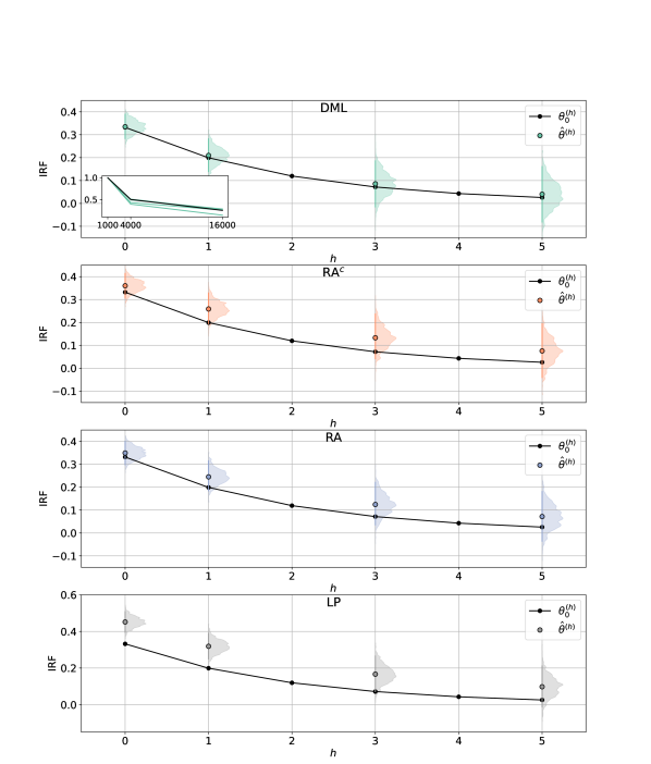
Figure 2: Comparison of the true $\theta_{0}^{(h)}$ with estimates $\hat{\theta}^{(h)}$ of the IRF obtained for the one-sample scenario from Table 1 with $k_{T}=20$, $T=16^{\prime}000$, $n=12$, $\sigma_{\epsilon}=1$, $d_{y}=0$ and $b=0$. For individual $h$, we show kernel density estimates of the distribution of $\hat{\theta}^{(h)}$ across $N=1^{\prime}000$ realizations. The dots indicate the average, and the vertical lines the (2.5%, 97.5%)-quantile range of the distribution. In the inset of the top panel, for the DML estimator, normalized biases as a function of $T$ are plotted for all forecast horizons $h$ and contrasted to the $\sqrt{T}$ scaling implied by Theorem 3 in black.

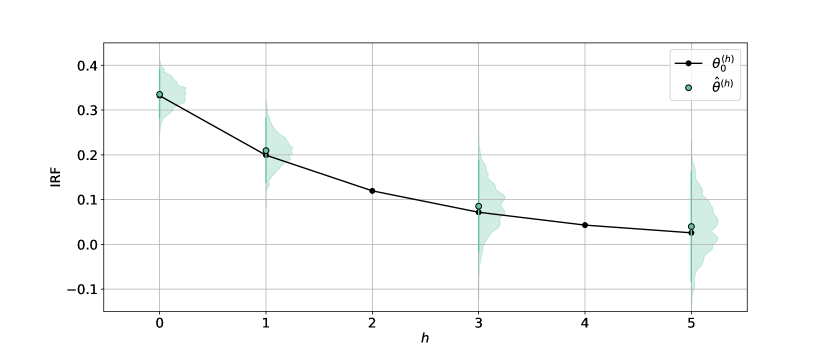
Figure D1: Comparison of the true $\theta_{0}^{(h)}$ with DML estimates $\hat{\theta}^{(h)}$ of the IRF. The DGP is a modification of the one-sample scenario from Table 1 with $k_{T}=20$, $T=$16’000, $n=12$ and $\sigma_{\epsilon}=1$, but $b=0$ and $d_{y}=0.4$. For individual $h$, we show kernel density estimates of the distribution of $\hat{\theta}^{(h)}$ across $N=1^{\prime}000$ realizations. The dots indicate the average, and the vertical lines the (2.5%, 97.5%)-quantile range of the distribution.

Finally, Figure D1 in Appendix D further documents results for the DML estimator on a DGP with $b=0$ and $d_{y}>0$. Also in a setup where Assumption 3-iv is violated, and the data used for estimation is not coming from an $\alpha$-mixing process, the DML estimator still delivers unbiased estimates of the IRF with valid confidence intervals, providing some limited evidence that assumption 3-iv might not be too strict in practice.

5 Empirical Application

To illustrate the methodology developed in the preceding sections, we apply it to the empirical study conducted in Angrist . (2018). Based on the same data set, we revisit the estimation of the average causal effect of US monetary policy decisions on macroeconomic aggregates using modern machine learning estimators.

Our monthly observations cover the period from July 1989 to December 2008 and we estimate the effect of federal funds target rate changes on a set of macroeconomic outcome variables. As predictors, we consider the same futures-based expectation measure for the federal funds rate as in Angrist . (2018), as well as the level of the target rate at the end of the prior month and its change, a scale factor that accounts for when within the month the Federal Reserve’s Open Market Committee (FOMC) meeting was scheduled, dummies for months with a scheduled FOMC meeting, as well as measures for inflation and unemployment (including lagged values). Compared to the setup in Angrist . (2018), we make the following modifications to accommodate for the change in estimation technique from linear models to flexible nonparametric machine learners. First, we exclude dummies for monthly fixed effects and special events like Y2K and the September 11, 2001 attacks, because IRF estimates are based on out-of-sample predictions in our approach. Second, we drop manually constructed interaction variables, as machine learning estimators are able to infer these effects from the data, if they are present.

Our treatment variable $D_{t}$ can assume one of five discrete values $d\in\{-0.5\%,-0.25\%,0,0.25\%,0.5\%\}$. The propensity score model for $e_{0}(d,x)=\Pr(D_{t}=d|X_{t}=x)$ is implemented as an ordinal classification (Frank  Hall, 2001). To estimate the conditional mean nuisance functions $\mu_{0}(d,x,h)$, we include the treatments as dummy variables in $X_{t}$ and tune/train one joint model for all types of treatments (an S-learner in the terminology of Künzel . (2019)). As in our simulation experiments in Section 4, we explore random forests and a gradient boosted trees algorithm as estimators for the nuisance functions. Details on tuning of the machine learners are provided in Appendix C. We apply our cross-fitting approach with $K=10$ and $k_{T}=24$, and remove the $k_{T}$ observations from the data used to estimate the machine learners.

We present estimated IRFs for the federal funds rate and the unemployment rate in Figure 3. Additionally, estimates for the effects on the bond yield curve are shown in Figure 4. In line with theory, the choice of estimation algorithm does not appear to substantively change results, and we thus focus on results based on random forest estimators, for 25 basis point decreases/increases of the target rate. Overall, we identify similar dynamics in the outcome variables as in Angrist . (2018). However, for the federal funds rate, we find a larger absolute effect for target rate decreases of around one percentage point that remains significant at the 5% level until around twenty months after the target rate decrease. This is compared to a peak effect of around 0.6 percentage points one year after a target rate increase, which becomes insignificant at the 5% level around that same time. Looking at the effects on the yield curve, in line with Angrist . (2018), we find that effects are less significant the longer the considered bond maturity. Changes in the federal funds target rate have a higher initial impact on short-term yields than on long-term yields, as expected. Contrary to Angrist . (2018), our estimates however do not suggest that term rates are less sensitive to policy accommodation than they are to tightening. In fact, the point estimate for the 3-month T-bill right after a target rate increase is around +0.1 percentage points, whereas for a target rate decrease it is around -0.3 percentage points, albeit with higher uncertainty and the 95% confidence interval ranging from -0.48 to -0.07 percentage points.

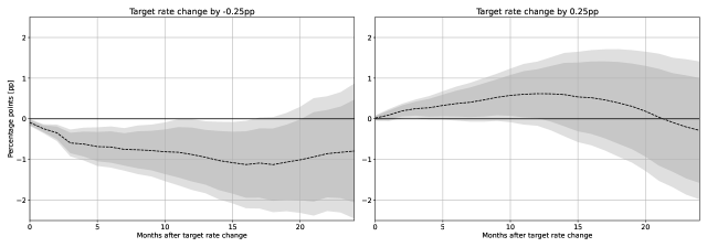
(a) Federal Funds Rate

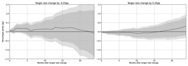
(b) Unemployment Rate

Figure 3: Estimated cumulative effects of target rate changes on (a) the federal funds rate and (b) the unemployment rate for the time period July 1989 to December 2008. The left (right) column shows the effect of decreasing (increasing) the target rate by 25 basis points. The shaded areas represent 95% and 99% confidence intervals according to (3).

Figure 4: Estimated cumulative effects of target rate changes on the bond yield curve for the time period July 1989 to December 2008.The left (right) column shows the effect of decreasing (increasing) the target rate by 25 basis points. The estimated effects on the yield curve are depicted for 0 (top row), 12 (middle row), and 24 (bottom row) months after the target rate change. The shaded areas represent 95% and 99% confidence intervals according to (3).

6 Conclusion

Estimation and inference of IRFs is a central task in many scientific disciplines. We have shown how to adopt recent ideas from the causal inference framework to flexibly estimate IRFs (Angrist ., 2018; Adamek ., 2024). This presents a novel estimator that can rely on fully nonparametric relations between treatment and outcome variables, opening up the possibility to use flexible machine learning approaches to estimate IRFs. As in the i.i.d. setting, the proposed estimator relies on the efficient influence function for the IRF in combination with cross-fitting. Our theoretical results outline conditions for this estimator to be consistent and asymptotically normally distributed at the parametric rate. Simulations where a highly nonlinear time series is treated over time corroborate these results, showing that the bias of the estimator decreases at the $\sqrt{T}$-rate and that it produces valid confidence intervals. Alternative approaches often used in practice estimate the IRF with a larger bias and fail to allow valid inference. Finally, we have illustrated the proposed methodology empirically by applying it to the estimation of the causal effects of macroeconomic shocks, allowing us to estimate IRFs of US monetary policy decisions on macroeconomic aggregates using modern machine learning estimators.

Future research could extend the proposed estimator in different directions. First, following the approach developed by Colangelo  Lee (2023) for i.i.d. data, one could extend the estimator to settings with continuous treatments. Second, to allow for even more flexibility in the estimated moment, the automatic debiased machine learning framework of Chernozhukov . (20221, 20222) could be brought to a time series setting. In a similar vein, an extension of the theory for semiparametric instrumental variable estimators (Chernozhukov ., 2018) to time series would be valuable in practice. Finally, our proposed estimator might be extended to the estimation of generalized IRFs by adapting Neyman-orthogonal conditional treatment effect estimators from an i.i.d. to a time series setting (Zimmert  Lechner, 2019; Qingliang Fan  Zhang, 2022; Semenova  Chernozhukov, 2020; Kennedy, 20232).

Appendix A Proofs

Proof of Theorem 1.

We have that

$$\mathbb{E}\left[Y_{t+h}(d)\right] =\mathbb{E}\left[\mathbb{E}\left[Y_{t+h}(d)|X_{t}\right]\right]$$

$$=\mathbb{E}\left[\mathbb{E}\left[Y_{t+h}(d)|D_{t}=d,X_{t}\right]\right]$$

$$=\mathbb{E}\left[\mathbb{E}\left[Y_{t+h}|D_{t}=d,X_{t}\right]\right]$$

$$=\mathbb{E}\left[\mu_{0}(d,X_{t},h)\right],$$

where the second equality follows from Assumption 2-i and the last equality from Assumption 2-ii. It thus follows that $\mathbb{E}\left[Y_{t+h}(1)-Y_{t+h}(0)\right]=\mathbb{E}\left[\mu_{0}(1,X_{t},h)-\mu_{0}(0,X_{t},h)\right]$. ∎

Proof of Theorem 2.

Under Assumption 3 the stochastic process $\mathcal{G}$ satisfies the assumptions for the Central Limit Theorem for $\alpha$-mixing processes (Herrndorf, 1984). ∎

Proof of Theorem 3.

The proof follows a similar strategy to the one in Wager (2022) and Chernozhukov . (2018) for the i.i.d. case. For the sake of legibility, we ease the notation and drop the reference to the forecast horizon $h$. Let $\tilde{\theta}$ be the oracle IRF estimator as defined in Theorem 2. Denote by $\mathcal{E}_{T}$ the event that $(\hat{\mu}_{S_{i}}(d,x,h),\hat{e}_{S_{i}}(x))\in\Xi_{T}^{(h)}$ for all $i\in\{1,2\}$. We have that

$$\sqrt{T}(\hat{\theta}-\theta_{0}) =\sqrt{T}(\hat{\theta}-\tilde{\theta}+\tilde{\theta}-\theta_{0})$$

$$=\sqrt{T}(\hat{\theta}-\tilde{\theta})+\sqrt{T}(\tilde{\theta}-\theta_{0})$$

$$=\sqrt{T}\left(\frac{|\mathcal{T}_{1}|}{T}\hat{\theta}_{S_{1}}+\frac{|\mathcal{T}_{2}|}{T}\hat{\theta}_{S_{2}}-\tilde{\theta}\right)+\sqrt{T}(\tilde{\theta}-\theta_{0})$$

$$=\sqrt{T}\left(\frac{|\mathcal{T}_{1}|}{T}\hat{\theta}_{S_{1}}+\frac{|\mathcal{T}_{2}|}{T}\hat{\theta}_{S_{2}}-\frac{|\mathcal{T}_{1}|}{T}\tilde{\theta}_{S_{1}}-\frac{|\mathcal{T}_{2}|}{T}\tilde{\theta}_{S_{2}}\right)+\sqrt{T}(\tilde{\theta}-\theta_{0})$$

$$=\sqrt{T}\left(\frac{|\mathcal{T}_{1}|}{T}\hat{\theta}_{S_{1}}-\frac{|\mathcal{T}_{1}|}{T}\tilde{\theta}_{S_{1}}\right)+\sqrt{T}\left(\frac{|\mathcal{T}_{2}|}{T}\hat{\theta}_{S_{2}}-\frac{|\mathcal{T}_{2}|}{T}\tilde{\theta}_{S_{2}}\right)+\sqrt{T}(\tilde{\theta}-\theta_{0}),$$

where $\tilde{\theta}_{S_{i}}=|\mathcal{T}_{i}|^{-1}\sum_{t\in\mathcal{T}_{i}}g(Z_{t};\Gamma_{0})$. We have to show that the first two terms converge to zero in probability. We will focus on the first term, the results for the second term immediately follow. We begin by expanding the first term as

$$\frac{|\mathcal{T}_{1}|}{T}\hat{\theta}_{S_{1}}-\frac{|\mathcal{T}_{1}|}{T}\tilde{\theta}_{S_{1}} =\frac{1}{|\mathcal{T}_{1}|}\sum_{t\in\mathcal{T}_{1}}g(Z_{t};\hat{\Gamma}_{S_{2}})-g(Z_{t};\Gamma_{0})$$

$$=\frac{1}{|\mathcal{T}_{1}|}\sum_{t\in\mathcal{T}_{1}}\left(\hat{\mu}_{S_{2}}(1,X_{t})-\mu_{0}(1,X_{t})+\frac{D_{t}}{\hat{e}_{S_{2}}(X_{t})}(Y_{t}-\hat{\mu}_{S_{2}}(1,X_{t}))-\frac{D_{t}}{{e}_{0}(X_{t})}(Y_{t}-{\mu}_{0}(1,X_{t}))\right)$$

$$\quad-\frac{1}{|\mathcal{T}_{1}|}\sum_{t\in\mathcal{T}_{1}}\bigg{(}\hat{\mu}_{S_{2}}(0,X_{t})-\mu_{0}(0,X_{t})+\frac{1-D_{t}}{1-\hat{e}_{S_{2}}(X_{t})}(Y_{t}-\hat{\mu}_{S_{2}}(0,X_{t}))$$

$$\qquad\qquad\qquad\qquad-\frac{1-D_{t}}{1-{e}_{0}(X_{t})}(Y_{t}-{\mu}_{0}(0,X_{t}))\bigg{)}.$$

We will prove convergence for the first summation, the second summation can be treated analogously. The first summation can be decomposed as

$$\frac{1}{|\mathcal{T}_{1}|}\sum_{t\in\mathcal{T}_{1}} \left(\hat{\mu}_{S_{2}}(1,X_{t})-\mu_{0}(1,X_{t})+\frac{D_{t}}{\hat{e}_{S_{2}}(X_{t})}(Y_{t}-\hat{\mu}_{S_{2}}(1,X_{t}))-\frac{D_{t}}{{e}_{0}(X_{t})}(Y_{t}-{\mu}_{0}(1,X_{t}))\right)$$

$$= \underbrace{\frac{1}{|\mathcal{T}_{1}|}\sum_{t\in\mathcal{T}_{1}}\left(\hat{\mu}_{S_{2}}(1,X_{t})-\mu_{0}(1,X_{t})\right)\left(1-\frac{D_{t}}{e_{0}(X_{t})}\right)}_{=P_{1}}$$

$$\quad+\underbrace{\frac{1}{|\mathcal{T}_{1}|}\sum_{t\in\mathcal{T}_{1}}D_{t}\left(Y_{t}-\mu_{0}(1,X_{t})\right)\left(\frac{1}{\hat{e}_{S_{2}}(X_{t})}-\frac{1}{e_{0}(X_{t})}\right)}_{=P_{2}}$$

$$\quad+\underbrace{\frac{1}{|\mathcal{T}_{1}|}\sum_{t\in\mathcal{T}_{1}}D_{t}\left(\hat{\mu}_{S_{2}}(1,X_{t})-\mu_{0}(1,X_{t})\right)\left(\frac{1}{\hat{e}_{S_{2}}(X_{t})}-\frac{1}{e_{0}(X_{t})}\right)}_{=P_{3}}.$$

We will show that $P_{i}=o_{p}(T^{-1/2})$, i.e. that $\sqrt{T}P_{i}\overset{p}{\to}0$ with measure $\mathcal{P}$ as $T\to\infty$, for $i\in\{1,2,3\}$.

Term $P_{1}$: From the squared $L_{2}$-norm of $P_{1}$ we have that

$$\mathbb{E}\Bigg{[} \Bigg{(}\frac{1}{|\mathcal{T}_{1}|}\sum_{t\in\mathcal{T}_{1}}\left(\hat{\mu}_{S_{2}}(1,X_{t})-\mu_{0}(1,X_{t})\right)\left(1-\frac{D_{t}}{e_{0}(X_{t})}\right)\Bigg{)}^{2}\Bigg{]}$$

$$=\frac{1}{|\mathcal{T}_{1}|^{2}}\mathbb{E}\left[\mathbb{E}\left[\left(\sum_{t\in\mathcal{T}_{1}}\left(\hat{\mu}_{S_{2}}(1,X_{t})-\mu_{0}(1,X_{t})\right)\left(1-\frac{D_{t}}{e_{0}(X_{t})}\right)\right)^{2}\Bigg{|}S_{2}\right]\right]$$

$$=\frac{1}{|\mathcal{T}_{1}|^{2}}\mathbb{E}\left[\mathrm{Var}\left[\sum_{t\in\mathcal{T}_{1}}\left(\hat{\mu}_{S_{2}}(1,X_{t})-\mu_{0}(1,X_{t})\right)\left(1-\frac{D_{t}}{e_{0}(X_{t})}\right)\Bigg{|}S_{2}\right]\right]$$

$$=\frac{1}{|\mathcal{T}_{1}|^{2}}\mathbb{E}\Bigg{[}\sum_{t\in\mathcal{T}_{1}}\sum_{s\in\mathcal{T}_{1}}\mathbb{E}\Bigg{[}\left(\hat{\mu}_{S_{2}}(1,X_{t})-\mu_{0}(1,X_{t})\right)\left(1-\frac{D_{t}}{e_{0}(X_{t})}\right)\times$$

$$\phantom{=\frac{1}{|\mathcal{T}_{1}|^{2}}\mathbb{E}\Bigg{[}\sum_{t\in\mathcal{T}_{1}}\sum_{s\in\mathcal{T}_{1}}\mathbb{E}\Bigg{[}}\left(\hat{\mu}_{S_{2}}(1,X_{s})-\mu_{0}(1,X_{s})\right)\left(1-\frac{D_{s}}{e_{0}(X_{s})}\right)\Bigg{|}S_{2}\Bigg{]}\Bigg{]}$$

$$=\frac{1}{|\mathcal{T}_{1}|^{2}}\mathbb{E}\left[\sum_{t\in\mathcal{T}_{1}}\mathbb{E}\left[\left(\hat{\mu}_{S_{2}}(1,X_{t})-\mu_{0}(1,X_{t})\right)^{2}\left(1-\frac{D_{t}}{e_{0}(X_{t})}\right)^{2}\Bigg{|}S_{2}\right]\right]$$

$$=\frac{1}{|\mathcal{T}_{1}|^{2}}\sum_{t\in\mathcal{T}_{1}}\mathbb{E}\left[\left(\hat{\mu}_{S_{2}}(1,X_{t})-\mu_{0}(1,X_{t})\right)^{2}\left(\frac{1}{e_{0}(X_{t})}-1\right)\right]$$

$$\leq\frac{1}{\eta|\mathcal{T}_{1}|^{2}}\sum_{t\in\mathcal{T}_{1}}\mathbb{E}\left[\left(\hat{\mu}_{S_{2}}(1,X_{t})-\mu_{0}(1,X_{t})\right)^{2}\right]=\frac{o_{p}(1)}{T}.$$

The third equality follows from the fact that the sum has mean zero and the inequality at the end follows from Assumption 4-iv. The step between the fourth and fifth equality follows from the fact that whenever $t<s$, we have that

$$\mathbb{E}\Bigg{[} \left(\hat{\mu}_{S_{2}}(1,X_{t})-\mu_{0}(1,X_{t})\right)\left(1-\frac{D_{t}}{e_{0}(X_{t})}\right)\left(\hat{\mu}_{S_{2}}(1,X_{s})-\mu_{0}(1,X_{s})\right)\left(1-\frac{D_{s}}{e_{0}(X_{s})}\right)\Bigg{|}S_{2}\Bigg{]}$$

$$=\mathbb{E}\Bigg{[}\left(\hat{\mu}_{S_{2}}(1,X_{t})-\mu_{0}(1,X_{t})\right)\left(1-\frac{D_{t}}{e_{0}(X_{t})}\right)\left(\hat{\mu}_{S_{2}}1(1,X_{s})-\mu_{0}(1,X_{s})\right)\times$$

$$\phantom{=\mathbb{E}\Bigg{[}}\;\underbrace{\mathbb{E}\left[1-\frac{D_{s}}{e_{0}(X_{s})}\Bigg{|}S_{2},\{X_{t}:t\in\mathcal{T}_{1},t\leq s\}\right]}_{=0}\Bigg{|}S_{2}\Bigg{]}=0.$$

The same argument can be made for $t>s$.

Convergence in the last step finally follows from the fact that $\lim_{T\to\infty}|\mathcal{T}_{1}|=\infty$ and by noting that conditional on $S_{2}$, the nuisance function estimator is non-stochastic, and thus conditional on the event $\mathcal{E}_{T}$, we have that

$$\sup_{t\in\mathcal{T}_{1}}\mathbb{E}\left[\left(\hat{\mu}_{S_{2}}(1,X_{t})-\mu_{0}(1,X_{t})\right)^{2}\Bigg{|}S_{2}\right] \leq\sup_{t\in\mathcal{T}_{1}}\sup_{\mu\in\Xi_{T}}\mathbb{E}\left[\left(\mu(1,X_{t})-\mu_{0}(1,X_{t})\right)^{2}\Bigg{|}S_{2}\right]$$

$$\leq\sup_{t\in\mathcal{T}_{1}}\sup_{\mu\in\Xi_{T}}\left\lVert\mu(1,X_{t})-\mu_{0}(1,X_{t})\right\rVert_{2}^{2}=o_{p}(1)$$

since by Assumption 4 $\sup_{t\in\mathcal{T}_{1}}\sup_{\mu\in\Xi_{T}}\left\lVert\mu(D_{t},X_{t})-\mu_{0}(D_{t},X_{t})\right\rVert_{2}^{2}=(r_{\mu,T})^{2}=o_{p}(1)$. By Lemma 6.1 in Chernozhukov . (2018) it follows that $\sup_{t\in\mathcal{T}_{1}}\mathbb{E}\left[\left(\hat{\mu}_{S_{2}}(1,X_{t})-\mu_{0}(1,X_{t})\right)^{2}\right]=o_{p}(1)$, and we thus conclude that $P_{1}$ is $o_{p}(T^{-1/2})$.

Term $P_{2}$: Similarly, from the squared $L_{2}$-norm of $P_{2}$ we have that

$$\mathbb{E}\Bigg{[} \Bigg{(}\frac{1}{|\mathcal{T}_{1}|}\sum_{t\in\mathcal{T}_{1}}D_{t}\left(Y_{t}-\mu_{0}(1,X_{t})\right)\left(\frac{1}{\hat{e}_{S_{2}}(X_{t})}-\frac{1}{e_{0}(X_{t})}\right)\Bigg{)}^{2}\Bigg{]}$$

$$=\frac{1}{|\mathcal{T}_{1}|^{2}}\mathbb{E}\Bigg{[}\mathbb{E}\Bigg{[}\Bigg{(}\sum_{t\in\mathcal{T}_{1}}D_{t}\left(Y_{t}-\mu_{0}(1,X_{t})\right)\left(\frac{1}{\hat{e}_{S_{2}}(X_{t})}-\frac{1}{e_{0}(X_{t})}\right)\Bigg{)}^{2}\Bigg{|}S_{2}\Bigg{]}\Bigg{]}$$

$$=\frac{1}{|\mathcal{T}_{1}|^{2}}\mathbb{E}\Bigg{[}\mathrm{Var}\Bigg{[}\sum_{t\in\mathcal{T}_{1}}D_{t}\left(Y_{t}-\mu_{0}(1,X_{t})\right)\left(\frac{1}{\hat{e}_{S_{2}}(X_{t})}-\frac{1}{e_{0}(X_{t})}\right)\Bigg{|}S_{2}\Bigg{]}\Bigg{]}$$

$$=\frac{1}{|\mathcal{T}_{1}|^{2}}\mathbb{E}\Bigg{[}\sum_{t\in\mathcal{T}_{1}}\sum_{s\in\mathcal{T}_{1}}\mathbb{E}\Bigg{[}D_{t}\left(Y_{t}-\mu_{0}(1,X_{t})\right)\left(\frac{1}{\hat{e}_{S_{2}}(X_{t})}-\frac{1}{e_{0}(X_{t})}\right)\times$$

$$\phantom{=\frac{1}{|\mathcal{T}_{1}|^{2}}\mathbb{E}\Bigg{[}\sum_{t\in\mathcal{T}_{1}}\sum_{s\in\mathcal{T}_{1}}\mathbb{E}\Bigg{[}}D_{s}\left(Y_{s}-\mu_{0}(1,X_{s})\right)\left(\frac{1}{\hat{e}_{S_{2}}(X_{s})}-\frac{1}{e_{0}(X_{s})}\right)\Bigg{|}S_{2}\Bigg{]}\Bigg{]}$$

$$=\frac{1}{|\mathcal{T}_{1}|^{2}}\mathbb{E}\Bigg{[}\sum_{t\in\mathcal{T}_{1}}\mathbb{E}\Bigg{[}D_{t}\left(Y_{t}-\mu_{0}(1,X_{t})\right)^{2}\left(\frac{1}{\hat{e}_{S_{2}}(X_{t})}-\frac{1}{e_{0}(X_{t})}\right)^{2}\Bigg{|}S_{2}\Bigg{]}\Bigg{]}$$

$$=\frac{1}{|\mathcal{T}_{1}|^{2}}\sum_{t\in\mathcal{T}_{1}}\mathbb{E}\Bigg{[}D_{t}\left(Y_{t}-\mu_{0}(1,X_{t})\right)^{2}\left(\frac{1}{\hat{e}_{S_{2}}(X_{t})}-\frac{1}{e_{0}(X_{t})}\right)^{2}\Bigg{]}$$

$$\leq\frac{1}{|\mathcal{T}_{1}|^{2}}\sum_{t\in\mathcal{T}_{1}}\mathbb{E}\Bigg{[}\left(Y_{t}-\mu_{0}(1,X_{t})\right)^{2}\left(\frac{1}{\hat{e}_{S_{2}}(X_{t})}-\frac{1}{e_{0}(X_{t})}\right)^{2}\Bigg{]}$$

$$\leq\frac{1}{|\mathcal{T}_{1}|^{2}}\epsilon^{2}_{1}\sum_{t\in\mathcal{T}_{1}}\mathbb{E}\Bigg{[}\left(\frac{1}{\hat{e}_{S_{2}}(X_{t})}-\frac{1}{e_{0}(X_{t})}\right)^{2}\Bigg{]}\leq\frac{1}{|\mathcal{T}_{1}|^{2}}\frac{\epsilon^{2}_{1}}{\eta^{2}}\sum_{t\in\mathcal{T}_{1}}\mathbb{E}\left[\left(\hat{e}_{S_{2}}(X_{t})-e_{0}(X_{t})\right)^{2}\right]=\frac{o_{p}(1)}{T}.$$

The third equality follows from the fact that the sum has mean zero, and the last three inequalities follow from iv and v in Assumption 4.

The crucial step is again to establish that the variance of the sum equals the sum of the variances (from equations four to five). This follows from the fact that whenever $t<s$, it holds that

$$\mathbb{E} \Bigg{[}D_{t}\left(Y_{t}-\mu_{0}(1,X_{t})\right)\left(\frac{1}{\hat{e}_{S_{2}}(X_{t})}-\frac{1}{e_{0}(X_{t})}\right)D_{s}\left(Y_{s}-\mu_{0}(1,X_{s})\right)\left(\frac{1}{\hat{e}_{S_{2}}(X_{s})}-\frac{1}{e_{0}(X_{s})}\right)\Bigg{|}S_{2}\Bigg{]}$$

$$=\mathbb{E}\Bigg{[}D_{t}\left(Y_{t}-\mu_{0}(1,X_{t})\right)\left(\frac{1}{\hat{e}_{S_{2}}(X_{t})}-\frac{1}{e_{0}(X_{t})}\right)\times$$

$$\phantom{\mathbb{E}\Bigg{[}D_{t}}\;\underbrace{\mathbb{E}\left[D_{s}(Y_{s}-\mu_{0}(1,X_{s}))\Bigg{|}S_{2},\{X_{t}:t\in\mathcal{T}_{1},t\leq s\}\right]}_{=0}\left(\frac{1}{\hat{e}_{S_{2}}(X_{s})}-\frac{1}{e_{0}(X_{s})}\right)\Bigg{|}S_{2}\Bigg{]}=0,$$

and the same argument can be made for $t>s$.

Convergence in the last step finally follows from the fact that $\lim_{T\to\infty}|\mathcal{T}_{1}|=\infty$ and by noting that conditional on $S_{2}$, the nuisance function estimator is non-stochastic, and thus conditional on the event $\mathcal{E}_{T}$, we have that

$$\sup_{t\in\mathcal{T}_{1}}\mathbb{E}\left[\left(\hat{e}_{S_{2}}(X_{t})-e_{0}(X_{t})\right)^{2}\Bigg{|}S_{2}\right] \leq\sup_{t\in\mathcal{T}_{1}}\sup_{e\in\Xi_{T}}\mathbb{E}\left[\left(e(X_{t})-e_{0}(X_{t})\right)^{2}\Bigg{|}S_{2}\right]$$

$$\leq\sup_{t\in\mathcal{T}_{1}}\sup_{e\in\Xi_{T}}\left\lVert e(X_{t})-e_{0}(X_{t})\right\rVert_{2}^{2}=(r_{e,T})^{2}$$

by definition of the rate $r_{e,T}$ in Assumption 4. By Lemma 6.1 in Chernozhukov . (2018) and Assumption 4 it follows that $\sup_{t\in\mathcal{T}_{1}}\mathbb{E}\left[\left(\hat{e}_{S_{2}}(X_{t})-e_{0}(X_{t})\right)^{2}\right]=o_{p}(1)$, and we thus conclude that $P_{2}$ is $o_{p}(T^{-1/2})$.

Term $P_{3}$: Finally, from the $L_{1}$-norm of $P_{3}$ we get that

$$\mathbb{E}\Bigg{[}\Bigg{|} \frac{1}{|\mathcal{T}_{1}|}\sum_{t\in\mathcal{T}_{1}}D_{t}\left(\hat{\mu}_{S_{2}}(1,X_{t})-\mu_{0}(1,X_{t})\right)\left(\frac{1}{\hat{e}_{S_{2}}(X_{t})}-\frac{1}{e_{0}(X_{t})}\right)\Bigg{|}\Bigg{]}$$

$$\leq\mathbb{E}\Bigg{[}\frac{1}{|\mathcal{T}_{1}|}\sum_{t\in\mathcal{T}_{1}}D_{t}\left|\hat{\mu}_{S_{2}}(1,X_{t})-\mu_{0}(1,X_{t})\right|\left|\frac{1}{\hat{e}_{S_{2}}(X_{t})}-\frac{1}{e_{0}(X_{t})}\right|\Bigg{]}$$

$$=\frac{1}{|\mathcal{T}_{1}|}\sum_{t\in\mathcal{T}_{1}}\mathbb{E}\Bigg{[}D_{t}\left|\hat{\mu}_{S_{2}}(1,X_{t})-\mu_{0}(1,X_{t})\right|\left|\frac{1}{\hat{e}_{S_{2}}(X_{t})}-\frac{1}{e_{0}(X_{t})}\right|\Bigg{]}$$

$$=\frac{1}{|\mathcal{T}_{1}|}\sum_{t\in\mathcal{T}_{1}}\mathbb{E}\Bigg{[}D_{t}\left|\hat{\mu}_{S_{2}}(D_{t},X_{t})-\mu_{0}(D_{t},X_{t})\right|\left|\frac{1}{\hat{e}_{S_{2}}(X_{t})}-\frac{1}{e_{0}(X_{t})}\right|\Bigg{]}$$

$$\leq\frac{1}{|\mathcal{T}_{1}|}\sum_{t\in\mathcal{T}_{1}}\mathbb{E}\Bigg{[}\left|\hat{\mu}_{S_{2}}(D_{t},X_{t})-\mu_{0}(D_{t},X_{t})\right|\left|\frac{1}{\hat{e}_{S_{2}}(X_{t})}-\frac{1}{e_{0}(X_{t})}\right|\Bigg{]}$$

$$\leq\frac{1}{\eta}\frac{1}{|\mathcal{T}_{1}|}\sum_{t\in\mathcal{T}_{1}}\mathbb{E}\Bigg{[}\left|\hat{\mu}_{S_{2}}(D_{t},X_{t})-\mu_{0}(D_{t},X_{t})\right|\left|\hat{e}_{S_{2}}(X_{t})-e_{0}(X_{t})\right|\Bigg{]}=\frac{o_{p}(1)}{T^{1/2}},$$

where the inequalities follow from Assumption 4-iv. Convergence in the last equality follows again from the fact that $\lim_{T\to\infty}|\mathcal{T}_{1}|=\infty$ and by noting that conditional on $S_{2}$, the nuisance function estimators are non-stochastic, and thus conditional on the event $\mathcal{E}_{T}$, we have that

$$\sup_{t\in\mathcal{T}_{1}}\mathbb{E}\Bigg{[} \left|\hat{\mu}_{S_{2}}(D_{t},X_{t})-\mu_{0}(D_{t},X_{t})\right|\left|\hat{e}_{S_{2}}(X_{t})-e_{0}(X_{t})\right|\Bigg{|}S_{2}\Bigg{]}$$

$$\leq\sup_{t\in\mathcal{T}_{1}}\mathbb{E}\Bigg{[}\left|\hat{\mu}_{S_{2}}(D_{t},X_{t})-\mu_{0}(D_{t},X_{t})\right|^{2}\Bigg{|}S_{2}\Bigg{]}^{1/2}\sup_{t\in\mathcal{T}_{1}}\mathbb{E}\Bigg{[}\left|\hat{e}_{S_{2}}(X_{t})-e_{0}(X_{t})\right|^{2}\Bigg{|}S_{2}\Bigg{]}^{1/2}$$

$$\leq\sup_{t\in\mathcal{T}_{1}}\sup_{\mu\in\Xi_{T}}\mathbb{E}\Bigg{[}\left|\mu(D_{t},X_{t})-\mu_{0}(D_{t},X_{t})\right|^{2}\Bigg{|}S_{2}\Bigg{]}^{1/2}\sup_{t\in\mathcal{T}_{1}}\sup_{e\in\Xi_{T}}\mathbb{E}\Bigg{[}\left|e(X_{t})-e_{0}(X_{t})\right|^{2}\Bigg{|}S_{2}\Bigg{]}^{1/2}$$

$$\leq\sup_{t\in\mathcal{T}_{1}}\sup_{\mu\in\Xi_{T}}\left\lVert\mu(D_{t},X_{t})-\mu_{0}(D_{t},X_{t})\right\rVert_{2}\sup_{t\in\mathcal{T}_{1}}\sup_{e\in\Xi_{T}}\left\lVert e(X_{t})-e_{0}(X_{t})\right\rVert_{2}=r_{\mu,T}\cdot r_{e,T}$$

by Cauchy-Schwarz and the definition of the rates $r_{\mu,T}$ and $r_{e,T}$ in Assumption 4. By Lemma 6.1 in Chernozhukov . (2018) and Assumption 4-iii it follows that $\sup_{t\in\mathcal{T}_{1}}\mathbb{E}\left[\left|\hat{\mu}_{S_{2}}(1,X_{t})-\mu_{0}(1,X_{t})\right|\left|\hat{e}_{S_{2}}(X_{t})-e_{0}(X_{t})\right|\right]=o_{p}(T^{-1/2})$.

We have shown that $P_{1}$, $P_{2}$ and $P_{3}$ are $o_{p}(T^{-1/2})$. It follows that

$$\frac{|\mathcal{T}_{1}|}{T}\hat{\theta}_{S_{1}}-\frac{|\mathcal{T}_{1}|}{T}\tilde{\theta}_{S_{1}}=o_{p}(T^{-1/2})$$

and applying similar arguments to $\frac{|\mathcal{T}_{2}|}{T}\hat{\theta}_{S_{2}}-\frac{|\mathcal{T}_{2}|}{T}\tilde{\theta}_{S_{2}}$, we can conclude that

$$\sqrt{T}(\hat{\theta}-\theta)=\underbrace{\sqrt{T}\left(\frac{|\mathcal{T}_{1}|}{T}\hat{\theta}_{S_{1}}-\frac{|\mathcal{T}_{1}|}{T}\tilde{\theta}_{S_{1}}\right)}_{=o_{p}(1)}+\underbrace{\sqrt{T}\left(\frac{|\mathcal{T}_{2}|}{T}\hat{\theta}_{S_{2}}-\frac{|\mathcal{T}_{2}|}{T}\tilde{\theta}_{S_{2}}\right)}_{=o_{p}(1)}+\underbrace{\sqrt{T}(\tilde{\theta}-\theta_{0})}_{\overset{d}{\to}\mathcal{N}(0,V_{0})}.$$

∎

Lemma A1.

Let $\Xi$ be a convex subset of some normed vector space, $g:\mathbb{R}^{n}\times\Xi\to\mathbb{R}$ be a measurable function, $\{Z_{t}:t\in\mathcal{T}\}$ an $\alpha$-mixing stochastic process with mixing coefficient $\alpha(m)$ and $Z_{t}$ a real-valued random vector. For $s\geq t$ denote by $\mathcal{F}_{t}^{s}=\sigma(Z_{t},\dots,Z_{s})$ the smallest $\sigma$-field such that $Z_{t},\dots,Z_{s}$ are measurable. If $\left\lVert\sup_{\Gamma\in\Xi}g(Z_{t},\Gamma)\right\rVert_{r}<\infty$ for some $r\geq p\geq 1$, then for all $t\in\mathcal{T}$

$$\sup_{\Gamma\in\Xi}\mathbb{E}\left[g(Z_{t},\Gamma)|\mathcal{F}^{t-k}_{-\infty}\right]=\sup_{\Gamma\in\Xi}\mathbb{E}\left[g(Z_{t},\Gamma)\right]+O_{p}(\alpha(k)^{1/p-1/r}).$$

Proof of Lemma A1.

We will prove the statement by bounding the $L_{p}$-norm. First notice that

$$\left\lVert\sup_{\Gamma\in\Xi}\mathbb{E}\left[g(Z_{t},\Gamma)|\mathcal{F}^{t-k}_{-\infty}\right]-\sup_{\Gamma\in\Xi}\mathbb{E}\left[g(Z_{t},\Gamma)\right]\right\rVert_{p}\leq\left\lVert\mathbb{E}\left[\sup_{\Gamma\in\Xi}\left(g(Z_{t},\Gamma)-\mathbb{E}\left[g(Z_{t},\Gamma)\right]\right)|\mathcal{F}^{t-k}_{-\infty}\right]\right\rVert_{p}$$

By Theorem 15.2 in Davidson (2021) we have

$$\left\lVert\mathbb{E}\left[\sup_{\Gamma\in\Xi}\left(g(Z_{t},\Gamma)-\mathbb{E}\left[g(Z_{t},\Gamma)\right]\right)|\mathcal{F}^{t-k}_{-\infty}\right]\right\rVert_{p} \leq 2(2^{1/2}+1)\alpha(k)^{1/p-1/r}\left\lVert\sup_{\Gamma\in\Xi}\left(g(Z_{t},\Gamma)-\mathbb{E}\left[g(Z_{t},\Gamma)\right]\right)\right\rVert_{r}$$

$$\leq 2(2^{1/2}+1)\alpha(k)^{1/p-1/r}\left(\left\lVert\sup_{\Gamma\in\Xi}g(Z_{t},\Gamma)\right\rVert_{r}+\left|\sup_{\Gamma\in\Xi}\mathbb{E}\left[g(Z_{t},\Gamma)\right]\right|\right)$$

$$=O(\alpha(k)^{1/p-1/r})$$

where the second inequality follows from the Minkowski inequality. ∎

Proof of Theorem 4.

The proof builds on the proof of Theorem 3. Without loss of generality, we will consider a stochastic process $\{Z_{t}:t\in\mathcal{T}\}$ with index set

$$\mathcal{T}=\left\{-\frac{T-1}{2},\dots,-1,0,1,\dots,\frac{T-1}{2}\right\}$$

such that $|\mathcal{T}|=T$. The index sets of the sub-processes are

$$\mathcal{T}_{1}=\left\{-\frac{T-1}{2},\dots,-\frac{k_{T}-1}{2}\right\}\quad\text{and}\qquad\mathcal{T}_{2}=\left\{\frac{k_{T}-1}{2},\dots,\frac{T-1}{2}\right\}.$$

Following the notation of Davidson (2021), let the $\mathcal{F}_{t}^{s}=\sigma(Z_{t},\dots,Z_{s})$ be the smallest $\sigma$-field on which the stochastic process coordinates from time $t$ to $s$ are measurable.

Consider the three summations $P_{1}$, $P_{2}$ and $P_{3}$ from the proof of Theorem 3.

Term $P_{1}$: From the squared $L_{2}$-norm of $P_{1}$ we to obtain

$$\begin{split}\mathbb{E}\Bigg{[}&\Bigg{(}\frac{1}{|\mathcal{T}_{1}|}\sum_{t\in\mathcal{T}_{1}}\left(\hat{\mu}_{S_{2}}(1,X_{t})-\mu_{0}(1,X_{t})\right)\left(1-\frac{D_{t}}{e_{0}(X_{t})}\right)\Bigg{)}^{2}\Bigg{]}\\ &=\frac{1}{|\mathcal{T}_{1}|^{2}}\sum_{t\in\mathcal{T}_{1}}\mathbb{E}\left[\left(\hat{\mu}_{S_{2}}(1,X_{t})-\mu_{0}(1,X_{t})\right)^{2}\left(1-\frac{D_{t}}{e_{0}(X_{t})}\right)^{2}\right]\\ &\phantom{=}+\frac{1}{|\mathcal{T}_{1}|^{2}}\sum_{t\in\mathcal{T}_{1}}\sum_{s\in\mathcal{T}_{1},s\neq t}\mathbb{E}\Bigg{[}\left(\hat{\mu}_{S_{2}}(1,X_{t})-\mu_{0}(1,X_{t})\right)\left(1-\frac{D_{t}}{e_{0}(X_{t})}\right)\times\\ &\phantom{=+\frac{1}{|\mathcal{T}_{1}|^{2}}\sum_{t\in\mathcal{T}_{1}}\sum_{s\in\mathcal{T}_{1},s\neq t}\mathbb{E}\Bigg{[}}\left(\hat{\mu}_{S_{2}}(1,X_{s})-\mu_{0}(1,X_{s})\right)\left(1-\frac{D_{s}}{e_{0}(X_{s})}\right)\Bigg{]}.\end{split}$$ (A1)

First, note that by applying Hölder’s inequality twice we have that for $r>p\geq 1$ and $1/r=1/r^{\prime}+1/r^{\prime\prime}$

$$\sup_{t,s\in\mathcal{T}_{1}}\sup_{\mu\in\Xi_{T}} \left\lVert\left(\mu(1,X_{t})-\mu_{0}(1,X_{t})\right)\left(1-\frac{D_{t}}{e_{0}(X_{t})}\right)\left(\mu(1,X_{s})-\mu_{0}(1,X_{s})\right)\left(1-\frac{D_{s}}{e_{0}(X_{s})}\right)\right\rVert_{r}$$

$$\leq\sup_{t\in\mathcal{T}_{1}}\sup_{\mu\in\Xi_{T}}\left\lVert\left(\mu(1,X_{t})-\mu_{0}(1,X_{t})\right)^{2}\left(1-\frac{D_{t}}{e_{0}(X_{t})}\right)^{2}\right\rVert_{r}$$

$$\leq\sup_{t\in\mathcal{T}_{1}}\sup_{\mu\in\Xi_{T}}\left\lVert\left(\mu(1,X_{t})-\mu_{0}(1,X_{t})\right)^{2}\right\rVert_{r^{\prime}}\left\lVert\left(1-\frac{D_{t}}{e_{0}(X_{t})}\right)^{2}\right\rVert_{r^{\prime\prime}}$$

which is bounded by Assumption 5-iii. Next, for the first summand in Equation (A1), note that conditional on $\mathcal{F}_{(k_{T}-1)/2}^{(T-1)/2}$ the estimator is non-stochastic, and thus conditional on the event $\mathcal{E}_{T}$ we have that

$$\sup_{t\in\mathcal{T}_{1}}\mathbb{E} \left[\left(\hat{\mu}_{S_{2}}(1,X_{t})-\mu_{0}(1,X_{t})\right)^{2}\left(1-\frac{D_{t}}{e_{0}(X_{t})}\right)^{2}\Bigg{|}\mathcal{F}_{(k_{T}-1)/2}^{(T-1)/2}\right]$$

$$\leq\sup_{t\in\mathcal{T}_{1}}\sup_{\mu\in\Xi_{T}}\mathbb{E}\left[\left(\mu(1,X_{t})-\mu_{0}(1,X_{t})\right)^{2}\left(1-\frac{D_{t}}{e_{0}(X_{t})}\right)^{2}\Bigg{|}\mathcal{F}_{(k_{T}-1)/2}^{(T-1)/2}\right]$$

$$\leq\sup_{t\in\mathcal{T}_{1}}\sup_{\mu\in\Xi_{T}}\mathbb{E}\left[\left(\mu(1,X_{t})-\mu_{0}(1,X_{t})\right)^{2}\left(1-\frac{D_{t}}{e_{0}(X_{t})}\right)^{2}\right]+O_{p}\left(\alpha(k_{T})^{\psi}\right)$$

$$=o_{p}(1)+O_{p}\left(\alpha(k_{T})^{\psi}\right)$$

by Lemma A1 in combination with Assumption 5, and the definition of the rate $r_{\mu,T}$ in Assumption 4. By Lemma 6.1 in Chernozhukov . (2018) and Assumptions 4-iii and 5-v it follows that

$$\frac{1}{|\mathcal{T}_{1}|^{2}}\sum_{t\in\mathcal{T}_{1}}\mathbb{E}\left[\left(\hat{\mu}_{S_{2}}(1,X_{t})-\mu_{0}(1,X_{t})\right)^{2}\left(1-\frac{D_{t}}{e_{0}(X_{t})}\right)^{2}\right]=\frac{o_{p}(1)}{|\mathcal{T}_{1}|}$$

Similarly, for the second summand of the $L_{2}$-norm of $P_{1}$, conditional on the event $\mathcal{E}_{T}$ we have that

$$\sup_{t,s\in\mathcal{T}_{1}}\mathbb{E}\Bigg{[} \left(\hat{\mu}_{S_{2}}(1,X_{t})-\mu_{0}(1,X_{t})\right)\left(1-\frac{D_{t}}{e_{0}(X_{t})}\right)\left(\hat{\mu}_{S_{2}}(1,X_{s})-\mu_{0}(1,X_{s})\right)\left(1-\frac{D_{s}}{e_{0}(X_{s})}\right)\Bigg{|}\mathcal{F}_{(k_{T}-1)/2}^{(T-1)/2}\Bigg{]}$$

$$\leq\sup_{t,s\in\mathcal{T}_{1}}\sup_{e\in\Xi_{T}}\mathbb{E}\bigg{[}\left(\mu(1,X_{t})-\mu_{0}(1,X_{t})\right)\left(1-\frac{D_{t}}{e_{0}(X_{t})}\right)\times$$

$$\qquad\qquad\qquad\qquad\left(\mu(1,X_{s})-\mu_{0}(1,X_{s})\right)\left(1-\frac{D_{s}}{e_{0}(X_{s})}\right)\Bigg{|}\mathcal{F}_{(k_{T}-1)/2}^{(T-1)/2}\bigg{]}$$

$$\leq\sup_{t,s\in\mathcal{T}_{1}}\sup_{e\in\Xi_{T}}\mathbb{E}\bigg{[}\left(\mu(1,X_{t})-\mu_{0}(1,X_{t})\right)\left(1-\frac{D_{t}}{e_{0}(X_{t})}\right)\times$$

$$\qquad\qquad\qquad\qquad\left(\mu(1,X_{s})-\mu_{0}(1,X_{s})\right)\left(1-\frac{D_{s}}{e_{0}(X_{s})}\right)\bigg{]}+O_{p}\left(\alpha(k_{T})^{\psi}\right)$$

by Lemma A1 in combination with Assumption 5, and the expectation in the last inequality is zero. By Lemma 6.1 in Chernozhukov . (2018) and Assumptions 4-iii and 5-v it follows that

$$\frac{1}{|\mathcal{T}_{1}|^{2}}\sum_{t\in\mathcal{T}_{1}}\sum_{s\in\mathcal{T}_{1},s\neq t}\mathbb{E}\Bigg{[}\left(\hat{\mu}_{S_{2}}(1,X_{t})-\mu_{0}(1,X_{t})\right)\left(1-\frac{D_{t}}{e_{0}(X_{t})}\right)\times$$

$$\qquad\qquad\qquad\qquad\qquad\left(\hat{\mu}_{S_{2}}(1,X_{s})-\mu_{0}(1,X_{s})\right)\left(1-\frac{D_{s}}{e_{0}(X_{s})}\right)\Bigg{]}=O_{p}\left(\alpha(k_{T})^{\psi}\right).$$

By Assumption 5-v it follows that $P_{1}$ is $o_{p}(T^{-1/2})$. Following a similar argument, it can be shown that $P_{2}$ is $o_{p}(T^{-1/2})$.

Convergence for $P_{3}$ can again be shown by bounding its $L_{1}$-norm as

$$\mathbb{E}\Bigg{[}\Bigg{|} \frac{1}{|\mathcal{T}_{1}|}\sum_{t\in\mathcal{T}_{1}}D_{t}\left(\hat{\mu}_{S_{2}}(1,X_{t})-\mu_{0}(1,X_{t})\right)\left(\frac{1}{\hat{e}_{S_{2}}(X_{t})}-\frac{1}{e_{0}(X_{t})}\right)\Bigg{|}\Bigg{]}$$

$$=\frac{1}{|\mathcal{T}_{1}|}\mathbb{E}\Bigg{[}\Bigg{|}\sum_{t\in\mathcal{T}_{1}}D_{t}\left(\hat{\mu}_{S_{2}}(D_{t},X_{t})-\mu_{0}(D_{t},X_{t})\right)\left(\frac{1}{\hat{e}_{S_{2}}(X_{t})}-\frac{1}{e_{0}(X_{t})}\right)\Bigg{|}\Bigg{]}$$

$$\leq\frac{1}{\eta}\frac{1}{|\mathcal{T}_{1}|}\sum_{t\in\mathcal{T}_{1}}\mathbb{E}\Bigg{[}\left|\hat{\mu}_{S_{2}}(D_{t},X_{t})-\mu_{0}(D_{t},X_{t})\right|\left|\hat{e}_{S_{2}}(X_{t})-e_{0}(X_{t})\right|\Bigg{]}.$$

Noting that conditional on $\mathcal{F}_{(k_{T}-1)/2}^{(T-1)/2}$, the nuisance function estimators are non-stochastic, and thus conditional on the event $\mathcal{E}_{T}$ we have that

$$\sup_{t\in\mathcal{T}_{1}}\mathbb{E}\Bigg{[} \left|\hat{\mu}_{S_{2}}(D_{t},X_{t})-\mu_{0}(D_{t},X_{t})\right|\left|\hat{e}_{S_{2}}(X_{t})-e_{0}(X_{t})\right|\Bigg{|}\mathcal{F}_{(k_{T}-1)/2}^{(T-1)/2}\Bigg{]}$$

$$\leq\sup_{t\in\mathcal{T}_{1}}\sup_{\mu,e\in\Xi_{T}}\mathbb{E}\Bigg{[}\left|\mu(D_{t},X_{t})-\mu_{0}(D_{t},X_{t})\right|\left|e(X_{t})-e_{0}(X_{t})\right|\Bigg{|}\mathcal{F}_{(k_{T}-1)/2}^{(T-1)/2}\Bigg{]}$$

$$\leq\sup_{t\in\mathcal{T}_{1}}\sup_{\mu,e\in\Xi_{T}}\mathbb{E}\Bigg{[}\left|\mu(D_{t},X_{t})-\mu_{0}(D_{t},X_{t})\right|\left|e(X_{t})-e_{0}(X_{t})\right|\Bigg{]}+O_{p}(\alpha(k_{T})^{\psi})$$

$$\leq\sup_{t\in\mathcal{T}_{1}}\sup_{\mu\in\Xi_{T}}\left\lVert\mu(D_{t},X_{t})-\mu_{0}(D_{t},X_{t})\right\rVert_{2}\sup_{t\in\mathcal{T}_{1}}\sup_{e\in\Xi_{T}}\left\lVert e(X_{t})-e_{0}(X_{t})\right\rVert_{2}+O_{p}(\alpha(k_{T})^{\psi})$$

$$=r_{\mu,T}\cdot r_{e,T}+O_{p}(\alpha(k_{T})^{\psi})$$

by Lemma A1 in combination with Assumption 5, Cauchy-Schwarz and the definition of the rates $r_{\mu,T}$ and $r_{e,T}$ in Assumption 4. By Lemma 6.1 in Chernozhukov . (2018) and Assumptions 4-iii and 5-v it follows that $\sup_{t\in\mathcal{T}_{1}}\mathbb{E}\left[\left|\hat{\mu}_{S_{2}}(1,X_{t})-\mu_{0}(1,X_{t})\right|\left|\hat{e}_{S_{2}}(X_{t})-e(X_{t})\right|\right]=o_{p}(T^{-1/2})$. This concludes the proof as we can now apply the same arguments as in the proof of Theorem 3. ∎

Proof of Theorem 5.

Define $v_{t}(\theta,\Gamma)=g(Z_{t};\Gamma)-\theta$, for some nuisance functions $\Gamma=(\mu,e)$, $g(Z_{t};\Gamma)$ is the influence function (2) evaluated using the nuisance functions in $\Gamma$ and we will drop the forecast horizon $h$ everywhere for legibility. Let

$$V_{T}=\mathrm{Var}\left(\frac{1}{\sqrt{T}}\sum_{t\in\mathcal{T}}g(Z_{t};\Gamma_{0})\right)=\frac{1}{T}\left(\sum_{t=1}^{T}\mathbb{E}[v_{t}^{2}]+2\sum_{s=1}^{T-1}\sum_{t=s+1}^{T}\mathbb{E}[v_{t}v_{t-s}]\right)$$ (A2)

with $v_{t}=g(Z_{t};\Gamma_{0})-\theta_{0}$ and $\Gamma_{0}=(\mu_{0},e_{0})$, and thus $\lim_{T\to\infty}V_{T}=V_{0}$.

Next, define

$$V_{S_{i}}=\frac{1}{|\mathcal{T}_{i}|}\left(\sum_{t\in\mathcal{T}_{i}}\mathbb{E}[v^{2}_{t}]+2\sum_{s\in\mathcal{T}_{i}}\sum_{t\in\mathcal{T}_{i,s}}\mathbb{E}[v_{t}v_{t-s}]\right)$$ (A3)

with $\mathcal{T}_{i,s}=\{t\in\mathcal{T}_{i}\,|\,t-s\geq\min(\mathcal{T}_{i})\}$ for $i\in\{1,2\}$.

Then we have that $\lim_{T\to\infty}V_{S_{i}}=\lim_{T\to\infty}V_{T}=V_{0}$, so for $|\widehat{V}-V_{T}|\overset{p}{\to}0$ it will be sufficient to show that

$$|\widehat{V}_{S_{i}}-V_{S_{i}}|=o_{p}(1),$$ (A4)

where

$$\widehat{V}_{S_{i}}=\frac{1}{|\mathcal{T}_{i}|}\left(\sum_{t\in\mathcal{T}_{i}}\hat{v}^{2}_{t}+2\sum_{s=1}^{m_{T}}w(s,m_{T})\sum_{t\in\mathcal{T}_{i,s}}\hat{v}_{t}\hat{v}_{t-s}\right)$$ (A5)

with

$$\hat{v}_{t}=g(Z_{t};\hat{\Gamma}_{t})-\hat{\theta}\qquad\text{and}\qquad\hat{\Gamma}_{t}=\begin{cases}\hat{\Gamma}_{S_{2}},&\mbox{if }t\in\mathcal{T}_{1}\\ \hat{\Gamma}_{S_{1}},&\mbox{if }t\in\mathcal{T}_{2}\end{cases}.$$

Moreover, let

$$V^{m}_{S_{i}}=\frac{1}{|\mathcal{T}_{i}|}\left(\sum_{t\in\mathcal{T}_{i}}v^{2}_{t}+2\sum_{s=1}^{m_{T}}w(s,m_{T})\sum_{t\in\mathcal{T}_{i,s}}v_{t}v_{t-s}\right).$$ (A6)

Applying the triangle inequality, we will follow Newey  West (1987) and prove that the following three terms converge to zero in probability

$$|\widehat{V}_{S_{i}}-V_{S_{i}}|\leq\underbrace{|\widehat{V}_{S_{i}}-V^{m}_{S_{i}}|}_{=P_{1}}+\underbrace{|V^{m}_{S_{i}}-\mathbb{E}[V^{m}_{S_{i}}]|}_{=P_{2}}+\underbrace{|\mathbb{E}[V^{m}_{S_{i}}]-V_{S_{i}}|}_{=P_{3}}.$$ (A7)

Since terms $P_{2}$ and $P_{3}$ do not contain any estimated quantities, they are $o_{p}(1)$ following the same arguments as in the proof of Theorem 2 in Newey  West (1987), provided that Assumptions 6 i-iii hold.

For the term $P_{1}$, define a function

$$f(\theta,r)=\frac{1}{|\mathcal{T}_{i}|}\sum_{t\in\mathcal{T}_{i}}v_{t}(\theta,\Gamma_{0}+r(\hat{\Gamma}_{t}-\Gamma_{0}))^{2}+\frac{2}{|\mathcal{T}_{i}|}\sum_{s=1}^{m_{T}}w(s,m_{T})\sum_{t\in\mathcal{T}_{i,s}}v_{t}(\theta,\Gamma_{0}+r(\hat{\Gamma}_{t}-\Gamma_{0}))v_{t-s}(\theta,\Gamma_{0}+r(\hat{\Gamma}_{t}-\Gamma_{0})),$$

so that $\widehat{V}_{S_{i}}=f(\hat{\theta},1)$ and $V^{m}_{S_{i}}=f(\theta_{0},0)$. By the multivariate mean-value theorem, for some $(\tilde{\theta},\tilde{r})$ on the line segment from $(\theta_{0},0)$ to $(\hat{\theta},1)$, on the event $\mathcal{E}_{T}$ we have

$$\widehat{V}_{S_{i}}-V^{m}_{S_{i}}=f(\hat{\theta},1)-f(\theta_{0},0)=\frac{\partial f}{\partial\theta}(\tilde{\theta},\tilde{r})(\hat{\theta}-\theta_{0})+\frac{\partial f}{\partial r}(\tilde{\theta},\tilde{r})$$

and by the triangle inequality

$$|\widehat{V}_{S_{i}}-V^{m}_{S_{i}}|\leq\underbrace{\left|\frac{\partial f}{\partial\theta}(\tilde{\theta},\tilde{r})(\hat{\theta}-\theta_{0})\right|}_{=P_{11}}+\underbrace{\left|\frac{\partial f}{\partial r}(\tilde{\theta},\tilde{r})\right|}_{=P_{12}}.$$ (A8)

We will show that both terms on the right hand side of (A8) are $o_{p}(1)$.

Term $P_{11}$: The partial derivative with respect to $\theta$ in $P_{11}$ is

$$\frac{\partial f}{\partial\theta}(\tilde{\theta},\tilde{r}) =-\frac{2}{|\mathcal{T}_{i}|}\sum_{t\in\mathcal{T}_{i}}v_{t}(\tilde{\theta},\Gamma_{0}+\tilde{r}(\hat{\Gamma}_{t}-\Gamma_{0}))$$

$$\qquad-\frac{2}{|\mathcal{T}_{i}|}\sum_{s=1}^{m_{T}}w(s,m_{T})\sum_{t\in\mathcal{T}_{i,s}}\left[v_{t}(\tilde{\theta},\Gamma_{0}+\tilde{r}(\hat{\Gamma}_{t}-\Gamma_{0}))+v_{t-s}(\tilde{\theta},\Gamma_{0}+\tilde{r}(\hat{\Gamma}_{t}-\Gamma_{0}))\right]$$

and thus

$$\left|\frac{\partial f}{\partial\theta}(\tilde{\theta},\tilde{r})\right|\leq 2\sup_{t\in\mathcal{T}_{i}}|v_{t}(\tilde{\theta},\Gamma_{0}+\tilde{r}(\hat{\Gamma}_{t}-\Gamma_{0}))|+4m_{T}\sup_{t\in\mathcal{T}_{i}}|v_{t}(\tilde{\theta},\Gamma_{0}+\tilde{r}(\hat{\Gamma}_{t}-\Gamma_{0}))|.$$

Then we get for $P_{11}$ that

$$\left|\frac{\partial f}{\partial\theta}(\tilde{\theta},\tilde{r})\right||\hat{\theta}-\theta_{0}|\leq \ 2\sup_{t\in\mathcal{T}_{i}}|v_{t}(\tilde{\theta},\Gamma_{0}+\tilde{r}(\hat{\Gamma}_{t}-\Gamma_{0}))|\cdot|\hat{\theta}-\theta_{0}|$$ (A9)

$$+4\frac{m_{T}}{\sqrt{T}}\sup_{t\in\mathcal{T}_{i}}|v_{t}(\tilde{\theta},\Gamma_{0}+\tilde{r}(\hat{\Gamma}_{t}-\Gamma_{0}))|\cdot\sqrt{T}|\hat{\theta}-\theta_{0}|.$$

By Theorem 4, on the event $\mathcal{E}_{T}$, $|\hat{\theta}-\theta_{0}|=o_{p}(1)$ and $\sqrt{T}(\hat{\theta}-\theta_{0})=O_{p}(1)$. Moreover, by Assumption 6-iii, $\lim_{T\to\infty}m_{T}/\sqrt{T}=0$. Thus it remains to show that on the event $\mathcal{E}_{T}$, $\sup_{t\in\mathcal{T}_{i}}|v_{t}(\tilde{\theta},\Gamma_{0}+\tilde{r}(\hat{\Gamma}_{t}-\Gamma_{0}))|$ remains bounded in probability.

By the triangular inequality we have that

$$\bigg{|}v_{t}(\tilde{\theta},\Gamma_{0}+\tilde{r}(\hat{\Gamma}_{t}-\Gamma_{0}))\bigg{|}=\bigg{|}g(Z_{t};\Gamma_{0}+\tilde{r}(\hat{\Gamma}_{t}-\Gamma_{0}))-\tilde{\theta}\bigg{|}\leq\bigg{|}g(Z_{t};\Gamma_{0}+\tilde{r}(\hat{\Gamma}_{t}-\Gamma_{0}))\bigg{|}+|\tilde{\theta}|.$$ (A10)

For the first term after the inequality in (A10) we have, for some $q>2$

$$\left\lVert g(Z_{t};\Gamma_{0}+\tilde{r}(\hat{\Gamma}_{t}-\Gamma_{0}))\right\rVert_{q} =\bigg{\lVert}\mu_{0}(1,X_{t})+\tilde{r}(\hat{\mu}_{t}(1,X_{t})-\mu_{0}(1,X_{t}))$$ (A11)

$$\qquad-\mu_{0}(0,X_{t})-\tilde{r}(\hat{\mu}_{t}(0,X_{t})-\mu_{0}(0,X_{t}))$$

$$\qquad+\frac{D_{t}}{e_{0}(X_{t})+\tilde{r}(\hat{e}_{t}(X_{t})-e_{0}(X_{t}))}(Y_{t}-\mu_{0}(1,X_{t})-\tilde{r}(\hat{\mu}_{t}(1,X_{t})-\mu_{0}(1,X_{t})))$$

$$\qquad-\frac{1-D_{t}}{1-e_{0}(X_{t})-\tilde{r}(\hat{e}_{t}(X_{t})-e_{0}(X_{t}))}(Y_{t}-\mu_{0}(0,X_{t})-\tilde{r}(\hat{\mu}_{t}(0,X_{t})-\mu_{0}(0,X_{t})))\bigg{\rVert}_{q}$$

$$\leq\left\lVert\mu_{0}(1,X_{t})\right\rVert_{q}+\tilde{r}\left\lVert\hat{\mu}_{t}(1,X_{t})-\mu_{0}(1,X_{t})\right\rVert_{q}+\left\lVert\mu_{0}(0,X_{t})\right\rVert_{q}+\tilde{r}\left\lVert\hat{\mu}_{t}(0,X_{t})-\mu_{0}(0,X_{t})\right\rVert_{q}$$

$$\qquad+\bigg{\lVert}\frac{D_{t}}{e_{0}(X_{t})+\tilde{r}(\hat{e}_{t}(X_{t})-e_{0}(X_{t}))}(Y_{t}-\mu_{0}(1,X_{t})-\tilde{r}(\hat{\mu}_{t}(1,X_{t})-\mu_{0}(1,X_{t})))\bigg{\rVert}_{q}$$

$$\qquad+\bigg{\lVert}\frac{1-D_{t}}{1-e_{0}(X_{t})-\tilde{r}(\hat{e}_{t}(X_{t})-e_{0}(X_{t}))}(Y_{t}-\mu_{0}(0,X_{t})-\tilde{r}(\hat{\mu}_{t}(0,X_{t})-\mu_{0}(0,X_{t})))\bigg{\rVert}_{q}$$

where

$$\hat{\mu}_{t}=\begin{cases}\hat{\mu}_{S_{2}},&\mbox{if }t\in\mathcal{T}_{1}\\ \hat{\mu}_{S_{1}},&\mbox{if }t\in\mathcal{T}_{2}\end{cases}\qquad\text{and}\qquad\hat{e}_{t}=\begin{cases}\hat{e}_{S_{2}},&\mbox{if }t\in\mathcal{T}_{1}\\ \hat{e}_{S_{1}},&\mbox{if }t\in\mathcal{T}_{2}\end{cases}.$$

From Assumptions 4 and 6-iv we have

$$\left\lVert\hat{\mu}_{t}(d,X_{t})-\mu_{0}(d,X_{t})\right\rVert_{q}\leq\frac{C}{\eta^{1/q}}\qquad\text{and}\qquad\left\lVert\mu_{0}(d,X_{t})\right\rVert_{q}\leq\frac{C}{\eta^{1/q}},$$ (A12)

for $q>2$, any $\hat{\Gamma}_{t}\in\Xi_{T}$ and $d\in\{0,1\}$, as shown in the proof of Theorem 5.1 in Chernozhukov . (2018).

Using these results, we get the following bound for $|\tilde{\theta}|$

$$|\tilde{\theta}|\leq|\tilde{\theta}-\theta_{0}|+|\theta_{0}|\leq|\hat{\theta}-\theta_{0}|+|\theta_{0}|\leq|\hat{\theta}-\theta_{0}|+2\frac{C}{\eta^{1/q}},$$

where $|\theta_{0}|\leq 2C/\eta^{1/q}$ follows from Assumption 4, as shown in the proof of Theorem 5.1 in Chernozhukov . (2018). From Theorem 4, it follows that $|\hat{\theta}-\theta_{0}|=o_{p}(1)$, so $|\tilde{\theta}|=O_{p}(1)$.

We continue with the term in the second line of the last inequality in (A11). For $q>2$, conditional on $\mathcal{E}_{T}$, we get

$$\bigg{\lVert}\frac{D_{t}}{e_{0}(X_{t})+\tilde{r}(\hat{e}_{t}(X_{t})-e_{0}(X_{t}))} (Y_{t}-\mu_{0}(1,X_{t})-\tilde{r}(\hat{\mu}_{t}(1,X_{t})-\mu_{0}(1,X_{t})))\bigg{\rVert}_{q}$$ (A13)

$$\leq\frac{1}{\eta}\bigg{\lVert}D_{t}(Y_{t}-\mu_{0}(1,X_{t})-\tilde{r}(\hat{\mu}_{t}(1,X_{t})-\mu_{0}(1,X_{t})))\bigg{\rVert}_{q}$$

$$\leq\frac{1}{\eta}\bigg{\lVert}Y_{t}-\mu_{0}(1,X_{t})-\tilde{r}(\hat{\mu}_{t}(1,X_{t})-\mu_{0}(1,X_{t}))\bigg{\rVert}_{q}$$

$$\leq\frac{1}{\eta}\left\lVert Y_{t}\right\rVert_{q}+\frac{1}{\eta}\left\lVert\mu_{0}(1,X_{t})\right\rVert_{q}+\frac{\tilde{r}}{\eta}\left\lVert\hat{\mu}_{t}(1,X_{t})-\mu_{0}(1,X_{t})\right\rVert_{q}$$

$$\leq\frac{1}{\eta}C+\frac{1}{\eta}\frac{C}{\eta^{1/q}}+\frac{\tilde{r}}{\eta}\frac{C}{\eta^{1/q}},$$

where the first inequality follows from Assumption 4. The second inequality follows from $D_{t}\in\{0,1\}$, and the third from the Minkowski inequality. The fourth follows from (A12).

For the term in the third line of the last inequality in (A11), we get for $q>2$ and conditional on $\mathcal{E}_{T}$ that

$$\bigg{\lVert}\frac{1-D_{t}}{1-e_{0}(X_{t})-\tilde{r}(\hat{e}_{t}(X_{t})-e_{0}(X_{t}))} (Y_{t}-\mu_{0}(0,X_{t})-\tilde{r}(\hat{\mu}_{t}(0,X_{t})-\mu_{0}(0,X_{t})))\bigg{\rVert}_{q}$$ (A14)

$$\leq\frac{1}{\eta}\bigg{\lVert}Y_{t}-\mu_{0}(0,X_{t})-\tilde{r}(\hat{\mu}_{t}(0,X_{t})-\mu_{0}(0,X_{t}))\bigg{\rVert}_{q}$$

$$\leq\frac{1}{\eta}C+\frac{1}{\eta}\frac{C}{\eta^{1/q}}+\frac{\tilde{r}}{\eta}\frac{C}{\eta^{1/q}},$$

using the same arguments as for the term in (A13).

Since all of the terms in the first line of the last inequality in (A11) are $L_{q}$-bounded, they are also $O_{p}(1)$ by Markov’s inequality. The same holds for (A13) and (A14), so we can conclude that all of the terms on the right-hand-side of the last inequality in (A11) are $O_{p}(1)$.

As a consequence, $\sup_{t\in\mathcal{T}_{i}}|v_{t}(\tilde{\theta},\Gamma_{0}+\tilde{r}(\hat{\Gamma}_{t}-\Gamma_{0}))|=O_{p}(1)$ in (A9) and thus $P_{11}=o_{p}(1)$.

Term $P_{12}$: From the partial derivative with respect to $r$ in $P_{12}$ we find

$$\left|\frac{\partial f}{\partial r}(\tilde{\theta},\tilde{r})\right| =\bigg{|}\frac{2}{|\mathcal{T}_{i}|}\sum_{t\in\mathcal{T}_{i}}v_{t}(\tilde{\theta},\Gamma_{0}+\tilde{r}(\hat{\Gamma}_{t}-\Gamma_{0}))\frac{\partial v_{t}}{\partial r}(\tilde{\theta},\Gamma_{0}+\tilde{r}(\hat{\Gamma}_{t}-\Gamma_{0}))$$

$$\qquad+\frac{2}{|\mathcal{T}_{i}|}\sum_{s=1}^{m_{T}}w(s,m_{T})\sum_{t\in\mathcal{T}_{i,s}}v_{t}(\tilde{\theta},\Gamma_{0}+\tilde{r}(\hat{\Gamma}_{t}-\Gamma_{0}))\frac{\partial v_{t-s}}{\partial r}(\tilde{\theta},\Gamma_{0}+\tilde{r}(\hat{\Gamma}_{t}-\Gamma_{0}))$$

$$\qquad+\frac{2}{|\mathcal{T}_{i}|}\sum_{s=1}^{m_{T}}w(s,m_{T})\sum_{t\in\mathcal{T}_{i,s}}v_{t-s}(\tilde{\theta},\Gamma_{0}+\tilde{r}(\hat{\Gamma}_{t}-\Gamma_{0}))\frac{\partial v_{t}}{\partial r}(\tilde{\theta},\Gamma_{0}+\tilde{r}(\hat{\Gamma}_{t}-\Gamma_{0}))\bigg{|}$$

$$\leq 2\sup_{t\in\mathcal{T}_{i}}|v_{t}(\tilde{\theta},\Gamma_{0}+\tilde{r}(\hat{\Gamma}_{t}-\Gamma_{0}))|\sup_{t\in\mathcal{T}_{i}}\left|\frac{\partial v_{t}}{\partial r}(\tilde{\theta},\Gamma_{0}+\tilde{r}(\hat{\Gamma}_{t}-\Gamma_{0}))\right|$$

$$\qquad+4\frac{m_{T}}{T^{1/4}}\sup_{t\in\mathcal{T}_{i}}|v_{t}(\tilde{\theta},\Gamma_{0}+\tilde{r}(\hat{\Gamma}_{t}-\Gamma_{0}))|\sup_{t\in\mathcal{T}_{i}}\left|\frac{\partial v_{t}}{\partial r}(\tilde{\theta},\Gamma_{0}+\tilde{r}(\hat{\Gamma}_{t}-\Gamma_{0}))\right|T^{1/4}.$$

From proving $P_{11}=o_{p}(1)$ we know that $\sup_{t\in\mathcal{T}_{i}}|v_{t}(\tilde{\theta},\Gamma_{0}+\tilde{r}(\hat{\Gamma}_{t}-\Gamma_{0}))|=O_{p}(1)$. Moreover, $m_{T}/T^{1/4}=o(1)$ by Assumption 6-iii.

Thus it remains to show that $\sup_{t\in\mathcal{T}_{i}}|\frac{\partial v_{t}}{\partial r}(\tilde{\theta},\Gamma_{0}+\tilde{r}(\hat{\Gamma}_{t}-\Gamma_{0}))|=o_{p}(T^{-1/4})$.

By the triangle inequality, we have

$$\sup_{t\in\mathcal{T}_{i}}\left|\frac{\partial v_{t}}{\partial r}(\tilde{\theta},\Gamma_{0}+\tilde{r}(\hat{\Gamma}_{t}-\Gamma_{0}))\right|\leq P_{12,A}+P_{12,B}+P_{12,C}+P_{12,D},$$ (A15)

where

$$P_{12,A} =\sup_{t\in\mathcal{T}_{i}}\left|\hat{\mu}_{t}(1,X_{t})-\mu_{0}(1,X_{t})-\left(\hat{\mu}_{t}(0,X_{t})-\mu_{0}(0,X_{t})\right)\right|$$

$$P_{12,B} =\sup_{t\in\mathcal{T}_{i}}\bigg{|}\frac{D_{t}}{\left(e_{0}(X_{t})+\tilde{r}(\hat{e}_{t}(X_{t})-e_{o}(X_{t}))\right)^{2}}\times$$

$$\qquad\quad\left(Y_{t}-\mu_{0}(1,X_{t})-\tilde{r}(\hat{\mu}_{t}(1,X_{t})-\mu_{0}(1,X_{t}))\right)\times$$

$$\qquad\quad\left(\hat{e}_{t}(X_{t})-e_{0}(X_{t})\right)\bigg{|}$$

$$P_{12,C} =\sup_{t\in\mathcal{T}_{i}}\left|\frac{1-D_{t}}{1-e_{0}(X_{t})-\tilde{r}(\hat{e}_{t}(X_{t})-e_{0}(X_{t}))}\left(\hat{\mu}_{t}(0,X_{t})-\mu_{0}(0,X_{t})\right)\right|$$

$$P_{12,D} =\sup_{t\in\mathcal{T}_{i}}\bigg{|}\frac{1-D_{t}}{\left((1-\tilde{r})(1-e_{0}(X_{t}))+\tilde{r}(1-\hat{e}_{t}(X_{t}))\right)^{2}}\times$$

$$\qquad\quad\left(Y_{t}-\mu_{0}(0,X_{t})+\tilde{r}(\hat{\mu}_{t}(0,X_{t})-\mu_{0}(0,X_{t}))\right)\times$$

$$\qquad\quad\left(\hat{e}_{t}(X_{t})-e_{0}(X_{t})\right)\bigg{|}.$$

For $P_{12,A}$, we first establish that on the event $\mathcal{E}_{T}$ for $d\in\{0,1\}$ we have

$$\sup_{t\in\mathcal{T}_{i}}\mathbb{E}\left[\left|\hat{\mu}_{t}(d,X_{t})-\mu_{0}(d,X_{t})\right|^{2}\bigg{|}S_{-i}\right] \leq\sup_{t\in\mathcal{T}_{i}}\sup_{\mu\in\Xi_{T}}\mathbb{E}\left[\left(\mu(d,X_{t})-\mu_{0}(d,X_{t})\right)^{2}\bigg{|}S_{-i}\right]$$ (A16)

$$\leq\sup_{t\in\mathcal{T}_{i}}\sup_{\mu\in\Xi_{T}}\mathbb{E}\left[\left(\mu(d,X_{t})-\mu_{0}(d,X_{t})\right)^{2}\right]+O_{p}(\alpha(k_{T})^{\psi})$$

$$\leq r_{\mu,T}^{2}+O_{p}(\alpha(k_{T})^{\psi})=o_{p}(T^{-1/2}),$$

where $S_{-i}=S_{2}$ if $i=1$ and $S_{-i}=S_{1}$ if $i=2$. The second inequality follows from Lemma A1, the third by the definition of the rate $r_{\mu,T}$ in Assumption 4. The final equality follows by Lemma 6.1 in Chernozhukov . (2018) and Assumptions 4-iii, 5-v and 6-v. We thus conclude that on the event $\mathcal{E}_{T}$,

$$\sup_{t\in\mathcal{T}_{i}}\left|\hat{\mu}_{t}(d,X_{t})-\mu_{0}(d,X_{t})\right|=o_{p}(T^{-1/4})$$ (A17)

and as a consequence

$$P_{12,A}\leq\sup_{t\in\mathcal{T}_{i}}\left|\hat{\mu}_{t}(1,X_{t})-\mu_{0}(1,X_{t})\right|+\sup_{t\in\mathcal{T}_{i}}\left|\hat{\mu}_{t}(0,X_{t})-\mu_{0}(0,X_{t})\right|=o_{p}(T^{-1/4}).$$

For $P_{12,B}$, we first establish that on the event $\mathcal{E}_{T}$ we have

$$\sup_{t\in\mathcal{T}_{i}}\mathbb{E}\left[\left|\hat{e}_{t}(X_{t})-e_{0}(X_{t})\right|^{2}\big{|}S_{-i}\right] \leq\sup_{t\in\mathcal{T}_{i}}\sup_{e\in\Xi_{T}}\mathbb{E}\left[(\hat{e}_{t}(X_{t})-e_{0}(X_{t}))^{2}\big{|}S_{-i}\right]$$

$$\leq\sup_{t\in\mathcal{T}_{i}}\sup_{e\in\Xi_{T}}\mathbb{E}\left[(\hat{e}_{t}(X_{t})-e_{0}(X_{t}))^{2}\right]+O_{p}(\alpha(k_{T})^{\psi})$$

$$\leq r_{e,T}^{2}+O_{p}(\alpha(k_{T})^{\psi})=o_{p}(T^{-1/2})$$

by the same arguments as for (A16) and thus on the event $\mathcal{E}_{T}$,

$$\sup_{t\in\mathcal{T}_{i}}\left|\hat{e}_{t}(X_{t})-e_{0}(X_{t})\right|=o_{p}(T^{-1/4}).$$ (A18)

This allows us to write

$$P_{12,B} \leq\sup_{t\in\mathcal{T}_{i}}\frac{1}{\eta^{2}}\left|Y_{t}-(1-\tilde{r})\mu_{0}(1,X_{t})-\tilde{r}\hat{\mu}_{t}(1,X_{t})\right|\left|\hat{e}_{t}(X_{t})-e_{0}(X_{t})\right|$$ (A19)

$$\leq\sup_{t\in\mathcal{T}_{i}}\frac{1-\tilde{r}}{\eta^{2}}\left|Y_{t}-\mu_{0}(1,X_{t})\right|\left|\hat{e}_{t}(X_{t})-e_{0}(X_{t})\right|+\sup_{t\in\mathcal{T}_{i}}\frac{\tilde{r}}{\eta^{2}}\left|Y_{t}-\hat{\mu}_{t}(1,X_{t})\right|\left|\hat{e}_{t}(X_{t})-e_{0}(X_{t})\right|$$

$$\leq\sup_{t\in\mathcal{T}_{i}}\frac{2}{\eta^{2}}\left|Y_{t}-\mu_{0}(1,X_{t})\right|\left|\hat{e}_{t}(X_{t})-e_{0}(X_{t})\right|+\sup_{t\in\mathcal{T}_{i}}\frac{1}{\eta^{2}}\left|\hat{\mu}_{t}(1,X_{t})-\mu_{0}(1,X_{t})\right|\left|\hat{e}_{t}(X_{t})-e_{0}(X_{t})\right|,$$

where the first inequality follows from Assumption 4 and $D_{t}\in\{0,1\}$.

From Assumption 6-iv and (A12), we have for $q>2$, $d\in\{0,1\}$ and any $\mu\in\Xi_{T}$ that

$$\sup_{t\in\mathcal{T}}\left\lVert Y_{t}-\mu(d,X_{t})\right\rVert_{q}\leq\sup_{t\in\mathcal{T}}\left\lVert Y_{t}\right\rVert_{q}+\sup_{t\in\mathcal{T}}\left\lVert\mu(d,X_{t})\right\rVert_{q}\leq C\left(1+\frac{1}{\eta^{1/q}}\right).$$ (A20)

Combined with (A18) it follows that for $d\in\{0,1\}$ and on the event $\mathcal{E}_{T}$ we have

$$\sup_{t\in\mathcal{T}_{i}}\left\lVert|Y_{t}-\mu(d,X_{t})||\hat{e}_{t}(X_{t})-e_{0}(X_{t})|\right\rVert_{1} \leq\sup_{t\in\mathcal{T}_{i}}\left\lVert Y_{t}-\mu(d,X_{t})\right\rVert_{2}\left\lVert\hat{e}_{t}(X_{t})-e_{0}(X_{t})\right\rVert_{2}$$

$$\leq\sup_{t\in\mathcal{T}_{i}}C\left(1+\frac{1}{\eta^{1/q}}\right)\left\lVert\hat{e}_{t}(X_{t})-e_{0}(X_{t})\right\rVert_{2}=o_{p}(T^{-1/4})$$

for any $\mu\in\Xi_{T}$, and as a consequence, combined with (A17), we have $P_{12,B}=o_{p}(T^{-1/4})$.

For $P_{12,C}$, we have by Assumption 4 and $D_{t}\in\{0,1\}$ that

$$P_{12,C}\leq\sup_{t\in\mathcal{T}_{i}}\frac{1}{\eta}|\hat{\mu}_{t}(0,X_{t})-\mu_{0}(0,X_{t})|$$

and thus $P_{12,C}=o_{p}(T^{-1/4})$ by (A17).

For $P_{12,D}$ finally, we have

$$P_{12,D} \leq\sup_{t\in\mathcal{T}_{i}}\frac{1}{\eta^{2}}\left|(1-\tilde{r})(Y_{t}-\mu_{0}(0,X_{t}))+\tilde{r}(Y_{t}-\hat{\mu}_{t}(0,X_{t}))\right|\left|\hat{e}_{t}(X_{t})-e_{0}(X_{t})\right|$$

$$\leq\sup_{t\in\mathcal{T}_{i}}\frac{2}{\eta^{2}}\left|Y_{t}-\mu_{0}(0,X_{t})\right|\left|\hat{e}_{t}(X_{t})-e_{0}(X_{t})\right|+\sup_{t\in\mathcal{T}_{i}}\frac{1}{\eta^{2}}\left|\hat{\mu}_{t}(0,X_{t})-\mu_{0}(0,X_{t})\right|\left|\hat{e}_{t}(X_{t})-e_{0}(X_{t})\right|,$$

where the first inequality again follows from Assumption 4 and $D_{t}\in\{0,1\}$, and the second from the same arguments as in (A19). Using (A17), (A18) and (A20) lets us conclude that $P_{12,D}=o_{p}(T^{-1/4})$.

This shows that all terms on the right hand side of (A15) are $o_{p}(T^{-1/4})$ and thus $\sup_{t\in\mathcal{T}_{i}}|\frac{\partial v_{t}}{\partial r}(\tilde{\theta},\Gamma_{0}+\tilde{r}(\hat{\Gamma}_{t}-\Gamma_{0}))|=o_{p}(T^{-1/4})$. As a consequence, $P_{11}=o_{p}(1)$ and $P_{12}=o_{p}(1)$ in (A8).

We conclude that $|\widehat{V}_{S_{i}}-V^{m}_{S_{i}}|=o_{p}(1)$ and thus $|\widehat{V}_{S_{i}}-V_{S_{i}}|=o_{p}(1)$ so that $|\widehat{V}-V_{T}|\overset{p}{\to}0$. ∎

Appendix B Hyperparameter tuning in the simulation study

Random forests: We fix the number of trees to 500. The maximal depth of each tree ($d$) and the minimal number of observations in the leafs of the trees ($\ell$) are determined by cross-validation on $R=10$ simulated samples. We perform a simple grid search over $\{\{d,\ell\}~{}\lvert~{}d\in\{10,20,50\}\wedge\ell\in\{1,5,10\}\}$ and select the hyperparameter-combination most frequently yielding the best predictive cross-validation performance (on $S_{2}$).

Gradient boosted trees: We perform a two-stage tuning procedure. In the first stage, we fix the learning rate of the tree booster to 0.1, set the number of boosting rounds to some very high number (10’000) and abort the training process (on $S_{1}$) if the predictive validation error (on $S_{2}$) has not decreased since 50 rounds of boosting. The maximum tree depth for the base learners ($d$), the minimum sum of instance weight needed in a child ($w$), the subsampling ratio for observations used to construct each tree ($s^{o}$), and the subsampling ratio for features when constructing each tree ($s^{f}$) are determined by cross-validation on $R=50$ simulated examples. We perform a simple grid search over $\{\{d,w,s^{o},s^{f}\}~{}\lvert~{}d\in\{1,...,10\}\wedge w\in\{1,...,10\}\wedge s^{o}\in\{0.25,0.5,0.75,1\}\wedge s^{f}\in\{0.25,0.5,0.75,1\}\}$ and select the hyperparameter-combination yielding the best predictive cross-validation performance (on $S_{2}$).

In the second stage, using the optimal tree-hyperparameters from stage 1, we select the learning rate most frequently yielding the best predictive cross-validation performance (on $S_{2}$) across an additional $R$ draws. We perform a search over the candidate set $\{0.001,0.002,0.005,0.01,0.02,0.05,0.1,0.25,0.5\}$. Finally, the optimal number of boosting rounds is determined as the average early-stopped boosting round for the selected learning rate.

Appendix C Hyperparameter tuning in the empirical application

Random forests: We fix the number of trees to 500. The maximal depth of each tree ($d$), the minimal number of observations in the leafs of the trees ($\ell$) and the size of the random subsets of features to consider when splitting a node ($\bar{m}$) are determined by cross-validation. We perform a simple grid search over $\{\{d,\ell,\bar{m}\}~{}\lvert~{}d\in\{1,2,3,4,5,10,20,30,40,50,100,200\}\wedge\ell\in\{1,2,3,4,5,10,20,30,40,50\}\}\wedge\bar{m}\in\{\sqrt{\mathrm{dim}(\mathcal{X})},\log_{2}\mathrm{dim}(\mathcal{X}),\mathrm{dim}(\mathcal{X})\}\}$ and select the hyperparameter-combination most frequently yielding the best predictive cross-validation performance.

Gradient boosted trees: We perform a two-stage tuning procedure. In the first stage, we fix the learning rate of the tree booster to 0.1, the number of boosting rounds to 500 and find optimal tree parameters by cross-validation. For this, we perform a simple grid search over $\{\{d,w,s^{o},s^{f}\}~{}\lvert~{}d\in\{1,...,10\}\wedge w\in\{1,...,10\}\wedge s^{o}\in\{0.25,0.5,0.75,1\}\wedge s^{f}\in\{0.25,0.5,0.75,1\}\}$, for the same parameters as in Appendix B, and select the hyperparameter-combination yielding the best predictive cross-validation performance.

In the second stage, using the optimal tree-hyperparameters from stage 1, we finally select the learning rate and number of boosting rounds yielding the best predictive cross-validation performance. We perform a search over all combinations of $\{0.001,0.002,0.005,0.01,0.02,0.05,0.1,0.25,0.5\}$ for the learning rate and $\{10,110,210,310,410,510\}$ for the number of boosting rounds.

All estimators are tuned using 10-fold blocked cross-validation on the full sample, where at the boundary of the folds 24 observations are dropped to eliminate dependence between the folds.

Appendix D Additional Tables and Figures

Table D1: Simulation results across $N=1^{\prime}000$ draws. The parameters of the DGP are, $\gamma=0.6$, $b=5$, $d_{y}=0$, $p=2$, $q=1$, $\sigma^{2}_{u}=1.0$, $\alpha_{A}=0.3$, $\alpha_{M}=0.3$, $\rho_{A}=0.35$, $\rho_{M}=0.7$. For the scenario with one sample, the split was conducted by removing $k_{T}=20$ observations between $S_{1}$ and $S_{2}$. C($\cdot$) in the tables denotes the coverage at the given confidence level.

One sample ($n=20$, $\sigma_{\epsilon}=1.0$)
$h=0$, $\theta_{0}^{(h)}=0.3333$
	DML					RAc					RA
$T$	Bias	std$(\hat{\theta}^{(h)})$	RMSE	C(95%)	C(99%)	Bias	std$(\hat{\theta}^{(h)})$	RMSE	C(95%)	C(99%)	Bias	std$(\hat{\theta}^{(h)})$	RMSE	C(95%)	C(99%)
1000	0.0342	0.1358	0.1400	0.9247	0.9840	0.1908	0.1434	0.2387	0.2715	0.4020	0.0980	0.1136	0.1500	0.6370	0.7875
4000	0.0109	0.0562	0.0572	0.9393	0.9890	0.0774	0.0581	0.0968	0.4600	0.6250	0.0432	0.0534	0.0687	0.7312	0.8732
16000	0.0026	0.0274	0.0275	0.9375	0.9915	0.0281	0.0278	0.0396	0.6555	0.7782	0.0164	0.0272	0.0317	0.7785	0.8980
$h=1$, $\theta_{0}^{(h)}=0.2000$
	DML					RAc					RA
$T$	Bias	std$(\hat{\theta}^{(h)})$	RMSE	C(95%)	C(99%)	Bias	std$(\hat{\theta}^{(h)})$	RMSE	C(95%)	C(99%)	Bias	std$(\hat{\theta}^{(h)})$	RMSE	C(95%)	C(99%)
1000	0.0547	0.1757	0.1840	0.9213	0.9822	0.2146	0.1711	0.2745	0.2845	0.3930	0.1227	0.1326	0.1807	0.4933	0.6398
4000	0.0245	0.0700	0.0742	0.9377	0.9838	0.1163	0.0705	0.1360	0.2305	0.3327	0.0778	0.0627	0.1000	0.4073	0.5278
16000	0.0136	0.0351	0.0377	0.9137	0.9725	0.0655	0.0349	0.0742	0.1412	0.2225	0.0496	0.0333	0.0598	0.2640	0.3860
$h=3$, $\theta_{0}^{(h)}=0.0720$
	DML					RAc					RA
$T$	Bias	std$(\hat{\theta}^{(h)})$	RMSE	C(95%)	C(99%)	Bias	std$(\hat{\theta}^{(h)})$	RMSE	C(95%)	C(99%)	Bias	std$(\hat{\theta}^{(h)})$	RMSE	C(95%)	C(99%)
1000	0.0751	0.2608	0.2714	0.9083	0.9770	0.1362	0.2308	0.2680	0.4472	0.5695	0.1022	0.1837	0.2103	0.5333	0.6705
4000	0.0303	0.1044	0.1087	0.9330	0.9815	0.1034	0.1031	0.1460	0.2762	0.3623	0.0812	0.0903	0.1215	0.3290	0.4382
16000	0.0191	0.0543	0.0575	0.9097	0.9690	0.0730	0.0522	0.0897	0.1395	0.1797	0.0619	0.0499	0.0795	0.1580	0.2195
$h=5$, $\theta_{0}^{(h)}=0.0259$
	DML					RAc					RA
$T$	Bias	std$(\hat{\theta}^{(h)})$	RMSE	C(95%)	C(99%)	Bias	std$(\hat{\theta}^{(h)})$	RMSE	C(95%)	C(99%)	Bias	std$(\hat{\theta}^{(h)})$	RMSE	C(95%)	C(99%)
1000	0.0874	0.3160	0.3279	0.9048	0.9712	0.0907	0.2586	0.2740	0.4963	0.6290	0.0846	0.2099	0.2264	0.5860	0.7258
4000	0.0307	0.1288	0.1324	0.9260	0.9780	0.0787	0.1217	0.1449	0.3053	0.4070	0.0691	0.1085	0.1286	0.3460	0.4535
16000	0.0183	0.0652	0.0677	0.9097	0.9775	0.0599	0.0616	0.0859	0.1855	0.2345	0.0544	0.0598	0.0809	0.2025	0.2592
One sample ($n=12$, $\sigma_{\epsilon}=3.0$)
$h=0$, $\theta_{0}^{(h)}=0.3321$
	DML					RAc					RA
$T$	Bias	std$(\hat{\theta}^{(h)})$	RMSE	C(95%)	C(99%)	Bias	std$(\hat{\theta}^{(h)})$	RMSE	C(95%)	C(99%)	Bias	std$(\hat{\theta}^{(h)})$	RMSE	C(95%)	C(99%)
1000	0.0144	0.2255	0.2260	0.9520	0.9890	0.2128	0.2290	0.3126	0.3450	0.4500	0.1075	0.1831	0.2123	0.5010	0.6350
4000	0.0029	0.1025	0.1025	0.9500	0.9860	0.0633	0.1008	0.1190	0.4610	0.5860	0.0289	0.0912	0.0957	0.5600	0.7160
16000	0.0025	0.0495	0.0495	0.9450	0.9850	0.0245	0.0483	0.0541	0.5340	0.6530	0.0133	0.0471	0.0489	0.5750	0.7060
$h=1$, $\theta_{0}^{(h)}=0.1992$
	DML					RAc					RA
$T$	Bias	std$(\hat{\theta}^{(h)})$	RMSE	C(95%)	C(99%)	Bias	std$(\hat{\theta}^{(h)})$	RMSE	C(95%)	C(99%)	Bias	std$(\hat{\theta}^{(h)})$	RMSE	C(95%)	C(99%)
1000	0.0336	0.3495	0.3511	0.9510	0.9910	0.2321	0.3431	0.4142	0.4140	0.5390	0.1282	0.2754	0.3038	0.4720	0.6040
4000	0.0130	0.1637	0.1642	0.9470	0.9870	0.0956	0.1536	0.1810	0.3760	0.4830	0.0575	0.1403	0.1517	0.4310	0.5180
16000	0.0112	0.0784	0.0792	0.9350	0.9850	0.0564	0.0761	0.0947	0.2890	0.3900	0.0416	0.0731	0.0841	0.3080	0.3980
$h=3$, $\theta_{0}^{(h)}=0.0717$
	DML					RAc					RA
$T$	Bias	std$(\hat{\theta}^{(h)})$	RMSE	C(95%)	C(99%)	Bias	std$(\hat{\theta}^{(h)})$	RMSE	C(95%)	C(99%)	Bias	std$(\hat{\theta}^{(h)})$	RMSE	C(95%)	C(99%)
1000	0.0464	0.5453	0.5473	0.9510	0.9900	0.1840	0.4882	0.5217	0.4880	0.6030	0.1158	0.4097	0.4257	0.4850	0.6030
4000	0.0197	0.2534	0.2542	0.9440	0.9900	0.0908	0.2238	0.2415	0.3690	0.4800	0.0657	0.2091	0.2192	0.3600	0.4800
16000	0.0161	0.1174	0.1185	0.9480	0.9860	0.0646	0.1109	0.1284	0.2460	0.3030	0.0527	0.1073	0.1196	0.2270	0.3110
$h=5$, $\theta_{0}^{(h)}=0.0258$
	DML					RAc					RA
$T$	Bias	std$(\hat{\theta}^{(h)})$	RMSE	C(95%)	C(99%)	Bias	std$(\hat{\theta}^{(h)})$	RMSE	C(95%)	C(99%)	Bias	std$(\hat{\theta}^{(h)})$	RMSE	C(95%)	C(99%)
1000	0.0632	0.6776	0.6805	0.9130	0.9840	0.1330	0.5471	0.5630	0.4570	0.5720	0.0950	0.4704	0.4799	0.4840	0.6140
4000	0.0236	0.2932	0.2941	0.9360	0.9900	0.0630	0.2518	0.2595	0.3730	0.4800	0.0541	0.2355	0.2416	0.3820	0.4690
16000	0.0179	0.1314	0.1326	0.9420	0.9880	0.0521	0.1245	0.1349	0.2530	0.3020	0.0473	0.1210	0.1300	0.2370	0.3160

Table D2: Simulation results for an identical setting as the one sample scenario in Table 1, but where the $\mu_{0}(d,x,h)$ and $e_{0}(x)$ are estimated using a gradient boosting algorithm.

One sample ($n=12$, $\sigma_{\epsilon}=1.0$)
$h=0$, $\theta_{0}^{(h)}=0.3321$
	DML					RAc					RA
$T$	Bias	std$(\hat{\theta}^{(h)})$	RMSE	C(95%)	C(99%)	Bias	std$(\hat{\theta}^{(h)})$	RMSE	C(95%)	C(99%)	Bias	std$(\hat{\theta}^{(h)})$	RMSE	C(95%)	C(99%)
1000	0.0440	0.1621	0.1680	0.9266	0.9816	0.1405	0.1887	0.2353	0.6774	0.8188	0.1393	0.1551	0.2084	0.7050	0.8438
4000	0.0147	0.0574	0.0592	0.9438	0.9906	0.0454	0.0654	0.0797	0.7364	0.8774	0.0518	0.0623	0.0810	0.7318	0.8680
16000	0.0017	0.0264	0.0265	0.9546	0.9914	0.0098	0.0271	0.0288	0.7978	0.9084	0.0107	0.0266	0.0287	0.7964	0.9034
$h=1$, $\theta_{0}^{(h)}=0.1992$
	DML					RAc					RA
$T$	Bias	std$(\hat{\theta}^{(h)})$	RMSE	C(95%)	C(99%)	Bias	std$(\hat{\theta}^{(h)})$	RMSE	C(95%)	C(99%)	Bias	std$(\hat{\theta}^{(h)})$	RMSE	C(95%)	C(99%)
1000	0.0615	0.1803	0.1905	0.9238	0.9828	0.1643	0.2079	0.2650	0.5458	0.6806	0.1528	0.1747	0.2321	0.5398	0.6814
4000	0.0280	0.0666	0.0722	0.9286	0.9870	0.0766	0.0802	0.1109	0.4332	0.5718	0.0948	0.0748	0.1208	0.3546	0.4890
16000	0.0087	0.0319	0.0331	0.9350	0.9876	0.0295	0.0333	0.0445	0.4084	0.5440	0.0303	0.0322	0.0442	0.4162	0.5420
$h=3$, $\theta_{0}^{(h)}=0.0717$
	DML					RAc					RA
$T$	Bias	std$(\hat{\theta}^{(h)})$	RMSE	C(95%)	C(99%)	Bias	std$(\hat{\theta}^{(h)})$	RMSE	C(95%)	C(99%)	Bias	std$(\hat{\theta}^{(h)})$	RMSE	C(95%)	C(99%)
1000	0.0794	0.2388	0.2517	0.9240	0.9796	0.1638	0.2546	0.3027	0.4438	0.5622	0.1554	0.2301	0.2776	0.3888	0.4886
4000	0.0351	0.1013	0.1072	0.9256	0.9796	0.0696	0.1156	0.1349	0.3354	0.4304	0.0848	0.1117	0.1402	0.2526	0.3230
16000	0.0144	0.0486	0.0506	0.9212	0.9840	0.0471	0.0503	0.0689	0.1788	0.2394	0.0497	0.0492	0.0700	0.1354	0.1786
$h=5$, $\theta_{0}^{(h)}=0.0258$
	DML					RAc					RA
$T$	Bias	std$(\hat{\theta}^{(h)})$	RMSE	C(95%)	C(99%)	Bias	std$(\hat{\theta}^{(h)})$	RMSE	C(95%)	C(99%)	Bias	std$(\hat{\theta}^{(h)})$	RMSE	C(95%)	C(99%)
1000	0.0850	0.2828	0.2953	0.9106	0.9798	0.1553	0.2879	0.3272	0.4360	0.5424	0.1474	0.2627	0.3013	0.3524	0.4500
4000	0.0356	0.1203	0.1255	0.9230	0.9796	0.0628	0.1347	0.1486	0.3182	0.4216	0.0724	0.1308	0.1495	0.2402	0.2998
16000	0.0156	0.0591	0.0611	0.9204	0.9832	0.0468	0.0606	0.0766	0.1718	0.2228	0.0486	0.0599	0.0771	0.1200	0.1572

References

- Adamek \BOthers. (\APACyear2024) \APACinsertmetastarAdamek2024{APACrefauthors}Adamek, R., Smeekes, S.\BCBL \BBA Wilms, I. \APACrefYearMonthDay2024. \BBOQ\APACrefatitleLocal Projection Inference in High Dimensions Local Projection Inference in High Dimensions.\BBCQ \APACjournalVolNumPagesThe Econometrics Journal1–20. {APACrefDOI} doi:10.1093/ectj/utae012 \PrintBackRefs\CurrentBib
- Angrist \BOthers. (\APACyear2018) \APACinsertmetastarAngrist2018{APACrefauthors}Angrist, J\BPBID., Jordà, Ò.\BCBL \BBA Kuersteiner, G\BPBIM. \APACrefYearMonthDay2018. \BBOQ\APACrefatitleSemiparametric Estimates of Monetary Policy Effects: String Theory Revisited Semiparametric Estimates of Monetary Policy Effects: String Theory Revisited.\BBCQ \APACjournalVolNumPagesJournal of Business & Economic Statistics363371–387. {APACrefDOI} doi:10.1080/07350015.2016.1204919 \PrintBackRefs\CurrentBib
- Bach \BOthers. (\APACyear2024) \APACinsertmetastarBach2024{APACrefauthors}Bach, P., Schacht, O., Chernozhukov, V., Klaassen, S.\BCBL \BBA Spindler, M. \APACrefYearMonthDay2024. \BBOQ\APACrefatitleHyperparameter Tuning for Causal Inference with Double Machine Learning: A Simulation Study Hyperparameter Tuning for Causal Inference with Double Machine Learning: A Simulation Study.\BBCQ \BIn F. Locatello \BBA V. Didelez (\BEDS), \APACrefbtitleProceedings of the Third Conference on Causal Learning and Reasoning Proceedings of the third conference on causal learning and reasoning (\BVOL 236, \BPGS 1065–1117). \APACaddressPublisherPMLR. \PrintBackRefs\CurrentBib
- Barnichon \BBA Brownlees (\APACyear2019) \APACinsertmetastarBarnichon2019{APACrefauthors}Barnichon, R.\BCBT \BBA Brownlees, C. \APACrefYearMonthDay2019. \BBOQ\APACrefatitleImpulse Response Estimation by Smooth Local Projections Impulse Response Estimation by Smooth Local Projections.\BBCQ \APACjournalVolNumPagesThe Review of Economics and Statistics1013522–530. {APACrefURL} https://doi.org/10.1162/rest_a_00778 {APACrefDOI} doi:10.1162/rest_a_00778 \PrintBackRefs\CurrentBib
- Belloni \BOthers. (\APACyear2017) \APACinsertmetastarBelloni2017{APACrefauthors}Belloni, A., Chernozhukov, V., Fernández-Val, I.\BCBL \BBA Hansen, C. \APACrefYearMonthDay2017. \BBOQ\APACrefatitleProgram Evaluation and Causal Inference With High-Dimensional Data Program Evaluation and Causal Inference With High-Dimensional Data.\BBCQ \APACjournalVolNumPagesEconometrica851233–298. {APACrefDOI} doi:10.3982/ECTA12723 \PrintBackRefs\CurrentBib
- Bergmeir \BBA Benítez (\APACyear2012) \APACinsertmetastarBergmeir2012{APACrefauthors}Bergmeir, C.\BCBT \BBA Benítez, J\BPBIM. \APACrefYearMonthDay2012. \BBOQ\APACrefatitleOn the use of cross-validation for time series predictor evaluation On the use of cross-validation for time series predictor evaluation.\BBCQ \APACjournalVolNumPagesInformation Sciences191192–213. {APACrefDOI} doi:10.1016/j.ins.2011.12.028 \PrintBackRefs\CurrentBib
- Bica \BOthers. (\APACyear2020) \APACinsertmetastarBica2020{APACrefauthors}Bica, I., Alaa, A.\BCBL \BBA Van Der Schaar, M. \APACrefYearMonthDay2020. \BBOQ\APACrefatitleTime Series Deconfounder: Estimating Treatment Effects over Time in the Presence of Hidden Confounders Time Series Deconfounder: Estimating Treatment Effects over Time in the Presence of Hidden Confounders.\BBCQ \BIn H\BPBID. III \BBA A. Singh (\BEDS), \APACrefbtitleProceedings of the 37th International Conference on Machine Learning Proceedings of the 37th international conference on machine learning (\BVOL 119, \BPGS 884–895). \APACaddressPublisherPMLR. {APACrefDOI} doi:10.5555/3524938.3525021 \PrintBackRefs\CurrentBib
- Bouchaud \BOthers. (\APACyear2018) \APACinsertmetastarBouchaud2018{APACrefauthors}Bouchaud, J\BHBIP., Bonart, J., Donier, J.\BCBL \BBA Gould, M. \APACrefYear2018. \APACrefbtitleTrades, Quotes and Prices: Financial Markets Under the Microscope Trades, quotes and prices: Financial markets under the microscope. \APACaddressPublisherCambridge University Press. {APACrefDOI} doi:10.1017/9781316659335 \PrintBackRefs\CurrentBib
- Breiman (\APACyear2001) \APACinsertmetastarBreiman2001{APACrefauthors}Breiman, L. \APACrefYearMonthDay2001. \BBOQ\APACrefatitleRandom forests Random forests.\BBCQ \APACjournalVolNumPagesMachine Learning455–32. {APACrefDOI} doi:10.1023/A:1010933404324 \PrintBackRefs\CurrentBib
- Bussmann \BOthers. (\APACyear2021) \APACinsertmetastarBussmann2021{APACrefauthors}Bussmann, B., Nys, J.\BCBL \BBA Latré, S. \APACrefYearMonthDay2021. \BBOQ\APACrefatitleNeural Additive Vector Autoregression Models for Causal Discovery in Time Series Neural Additive Vector Autoregression Models for Causal Discovery in Time Series.\BBCQ \BIn C. Soares \BBA L. Torgo (\BEDS), \APACrefbtitleDiscovery Science Discovery Science (\BPGS 446–460). \APACaddressPublisherChamSpringer International Publishing. {APACrefDOI} doi:10.1007/978-3-030-88942-5_35 \PrintBackRefs\CurrentBib
- Caruana (\APACyear1997) \APACinsertmetastarCaruana1997{APACrefauthors}Caruana, R. \APACrefYearMonthDay1997. \BBOQ\APACrefatitleMultitask Learning Multitask Learning.\BBCQ \APACjournalVolNumPagesMachine Learning2841–75. {APACrefDOI} doi:10.1023/A:1007379606734 \PrintBackRefs\CurrentBib
- T. Chen \BBA Guestrin (\APACyear2016) \APACinsertmetastarChen2016{APACrefauthors}Chen, T.\BCBT \BBA Guestrin, C. \APACrefYearMonthDay2016. \BBOQ\APACrefatitleXGBoost: A Scalable Tree Boosting System XGBoost: A Scalable Tree Boosting System.\BBCQ \BIn \APACrefbtitleProceedings of the 22nd ACM SIGKDD International Conference on Knowledge Discovery and Data Mining Proceedings of the 22nd ACM SIGKDD International Conference on Knowledge Discovery and Data Mining (\BPG 785–-794). \APACaddressPublisherNew York, NY, USAAssociation for Computing Machinery. {APACrefDOI} doi:10.1145/2939672.2939785 \PrintBackRefs\CurrentBib
- X. Chen \BBA Christensen (\APACyear2015) \APACinsertmetastarCHEN2015447{APACrefauthors}Chen, X.\BCBT \BBA Christensen, T\BPBIM. \APACrefYearMonthDay2015. \BBOQ\APACrefatitleOptimal uniform convergence rates and asymptotic normality for series estimators under weak dependence and weak conditions Optimal uniform convergence rates and asymptotic normality for series estimators under weak dependence and weak conditions.\BBCQ \APACjournalVolNumPagesJournal of Econometrics1882447–465. {APACrefURL} https://doi.org/10.1016/j.jeconom.2015.03.010 {APACrefDOI} doi:10.1016/j.jeconom.2015.03.010 \PrintBackRefs\CurrentBib
- Chernozhukov \BOthers. (\APACyear2017) \APACinsertmetastarChernozhukov2017AER{APACrefauthors}Chernozhukov, V., Chetverikov, D., Demirer, M., Duflo, E., Hansen, C.\BCBL \BBA Newey, W. \APACrefYearMonthDay2017. \BBOQ\APACrefatitleDouble/Debiased/Neyman Machine Learning of Treatment Effects Double/debiased/neyman machine learning of treatment effects.\BBCQ \APACjournalVolNumPagesAmerican Economic Review1075261–265. {APACrefDOI} doi:10.1257/aer.p20171038 \PrintBackRefs\CurrentBib
- Chernozhukov \BOthers. (\APACyear2018) \APACinsertmetastarChernozhukov2018{APACrefauthors}Chernozhukov, V., Chetverikov, D., Demirer, M., Duflo, E., Hansen, C., Newey, W.\BCBL \BBA Robins, J. \APACrefYearMonthDay2018. \BBOQ\APACrefatitleDouble/debiased machine learning for treatment and structural parameters Double/debiased machine learning for treatment and structural parameters.\BBCQ \APACjournalVolNumPagesThe Econometrics Journal211C1–C68. {APACrefDOI} doi:10.1111/ectj.12097 \PrintBackRefs\CurrentBib
- Chernozhukov \BOthers. (\APACyear2022\APACexlab\BCnt1) \APACinsertmetastarChernozhukov2022{APACrefauthors}Chernozhukov, V., Newey, W\BPBIK.\BCBL \BBA Singh, R. \APACrefYearMonthDay2022\BCnt1. \BBOQ\APACrefatitleAutomatic Debiased Machine Learning of Causal and Structural Effects Automatic Debiased Machine Learning of Causal and Structural Effects.\BBCQ \APACjournalVolNumPagesEconometrica903967–1027. {APACrefDOI} doi:10.3982/ECTA18515 \PrintBackRefs\CurrentBib
- Chernozhukov \BOthers. (\APACyear2022\APACexlab\BCnt2) \APACinsertmetastarChernozhukov2022b{APACrefauthors}Chernozhukov, V., Newey, W\BPBIK.\BCBL \BBA Singh, R. \APACrefYearMonthDay2022\BCnt2. \BBOQ\APACrefatitleDebiased machine learning of global and local parameters using regularized Riesz representers Debiased machine learning of global and local parameters using regularized Riesz representers.\BBCQ \APACjournalVolNumPagesThe Econometrics Journal253576–601. {APACrefDOI} doi:10.1093/ectj/utac002 \PrintBackRefs\CurrentBib
- Cochran (\APACyear1968) \APACinsertmetastarCochran1968{APACrefauthors}Cochran, W\BPBIG. \APACrefYearMonthDay1968. \BBOQ\APACrefatitleThe effectiveness of adjustment by subclassification in removing bias in observational studies The effectiveness of adjustment by subclassification in removing bias in observational studies.\BBCQ \APACjournalVolNumPagesBiometrics242295–313. {APACrefDOI} doi:10.2307/2528036 \PrintBackRefs\CurrentBib
- Colangelo \BBA Lee (\APACyear2023) \APACinsertmetastarColangelo2023{APACrefauthors}Colangelo, K.\BCBT \BBA Lee, Y\BHBIY. \APACrefYearMonthDay2023. \APACrefbtitleDouble Debiased Machine Learning Nonparametric Inference with Continuous Treatments. Double Debiased Machine Learning Nonparametric Inference with Continuous Treatments. \APACrefnotePreprint (arXiv:2004.03036) \PrintBackRefs\CurrentBib
- Davidson (\APACyear2021) \APACinsertmetastarDavidson2021{APACrefauthors}Davidson, J. \APACrefYear2021. \APACrefbtitleStochastic Limit Theory: An Introduction for Econometricians Stochastic Limit Theory: An Introduction for Econometricians (\PrintOrdinal2 \BEd). \APACaddressPublisherOxford University Press. {APACrefDOI} doi:10.1093/oso/9780192844507.001.0001 \PrintBackRefs\CurrentBib
- Farrell \BOthers. (\APACyear2021) \APACinsertmetastarFarrel2021{APACrefauthors}Farrell, M\BPBIH., Liang, T.\BCBL \BBA Misra, S. \APACrefYearMonthDay2021. \BBOQ\APACrefatitleDeep Neural Networks for Estimation and Inference Deep Neural Networks for Estimation and Inference.\BBCQ \APACjournalVolNumPagesEconometrica891181–213. {APACrefDOI} doi:10.3982/ECTA16901 \PrintBackRefs\CurrentBib
- Fisher \BBA Kennedy (\APACyear2021) \APACinsertmetastarFisher2021{APACrefauthors}Fisher, A.\BCBT \BBA Kennedy, E\BPBIH. \APACrefYearMonthDay2021. \BBOQ\APACrefatitleVisually Communicating and Teaching Intuition for Influence Functions Visually Communicating and Teaching Intuition for Influence Functions.\BBCQ \APACjournalVolNumPagesThe American Statistician752162–172. {APACrefDOI} doi:10.1080/00031305.2020.1717620 \PrintBackRefs\CurrentBib
- Frank \BBA Hall (\APACyear2001) \APACinsertmetastarOrdinalClassification2001{APACrefauthors}Frank, E.\BCBT \BBA Hall, M. \APACrefYearMonthDay2001. \BBOQ\APACrefatitleA Simple Approach to Ordinal Classification A Simple Approach to Ordinal Classification.\BBCQ \BIn L. De Raedt \BBA P. Flach (\BEDS), \APACrefbtitleMachine Learning: ECML 2001 Machine learning: Ecml 2001 (\BPGS 145–156). \APACaddressPublisherSpringer Berlin Heidelberg. \PrintBackRefs\CurrentBib
- Goehry, Benjamin (\APACyear2020) \APACinsertmetastarGoehry2020{APACrefauthors}Goehry, Benjamin. \APACrefYearMonthDay2020. \BBOQ\APACrefatitleRandom forests for time-dependent processes Random forests for time-dependent processes.\BBCQ \APACjournalVolNumPagesESAIM: PS24801–826. {APACrefDOI} doi:10.1051/ps/2020015 \PrintBackRefs\CurrentBib
- Grecov \BOthers. (\APACyear2021) \APACinsertmetastarGrecov2021{APACrefauthors}Grecov, P., Bandara, K., Bergmeir, C., Ackermann, K., Campbell, S., Scott, D.\BCBL \BBA Lubman, D. \APACrefYearMonthDay2021. \BBOQ\APACrefatitleCausal Inference Using Global Forecasting Models for Counterfactual Prediction Causal Inference Using Global Forecasting Models for Counterfactual Prediction.\BBCQ \BIn K. Karlapalem \BOthers. (\BEDS), \APACrefbtitleAdvances in Knowledge Discovery and Data Mining Advances in Knowledge Discovery and Data Mining (\BPGS 282–294). \APACaddressPublisherChamSpringer International Publishing. {APACrefDOI} doi:10.1007/978-3-030-75765-6_23 \PrintBackRefs\CurrentBib
- Hahn (\APACyear1998) \APACinsertmetastarHahn1998{APACrefauthors}Hahn, J. \APACrefYearMonthDay1998. \BBOQ\APACrefatitleOn the Role of the Propensity Score in Efficient Semiparametric Estimation of Average Treatment Effects On the Role of the Propensity Score in Efficient Semiparametric Estimation of Average Treatment Effects.\BBCQ \APACjournalVolNumPagesEconometrica662315–331. {APACrefDOI} doi:10.2307/2998560 \PrintBackRefs\CurrentBib
- Helson \BBA Sarason (\APACyear1967) \APACinsertmetastarHelsonSarason1967{APACrefauthors}Helson, H.\BCBT \BBA Sarason, D. \APACrefYearMonthDay1967. \BBOQ\APACrefatitlePast and Future Past and Future.\BBCQ \APACjournalVolNumPagesMathematica Scandinavia215–16. {APACrefDOI} doi:10.7146/math.scand.a-10840 \PrintBackRefs\CurrentBib
- Herrndorf (\APACyear1984) \APACinsertmetastarherrndorf1984{APACrefauthors}Herrndorf, N. \APACrefYearMonthDay1984. \BBOQ\APACrefatitleA functional central limit theorem for weakly dependent sequences of random variables A functional central limit theorem for weakly dependent sequences of random variables.\BBCQ \APACjournalVolNumPagesThe Annals of Probability141–153. {APACrefDOI} doi:10.1214/aop/1176993379 \PrintBackRefs\CurrentBib
- Irle (\APACyear1997) \APACinsertmetastarIrle1997{APACrefauthors}Irle, A. \APACrefYearMonthDay1997. \BBOQ\APACrefatitleOn Consistency in Nonparametric Estimation under Mixing Conditions On Consistency in Nonparametric Estimation under Mixing Conditions.\BBCQ \APACjournalVolNumPagesJournal of Multivariate Analysis601123–147. {APACrefDOI} doi:10.1006/jmva.1996.1647 \PrintBackRefs\CurrentBib
- Jordà (\APACyear2005) \APACinsertmetastarJorda2005{APACrefauthors}Jordà, Ò. \APACrefYearMonthDay2005. \BBOQ\APACrefatitleEstimation and Inference of Impulse Responses by Local Projections Estimation and Inference of Impulse Responses by Local Projections.\BBCQ \APACjournalVolNumPagesThe American Economic Review951161–182. {APACrefDOI} doi:10.1257/0002828053828518 \PrintBackRefs\CurrentBib
- Jordà (\APACyear2023) \APACinsertmetastarJorda2023{APACrefauthors}Jordà, Ò. \APACrefYearMonthDay2023. \BBOQ\APACrefatitleLocal Projections for Applied Economics Local Projections for Applied Economics.\BBCQ \APACjournalVolNumPagesAnnual Review of Economics15607–631. {APACrefDOI} doi:10.1146/annurev-economics-082222-065846 \PrintBackRefs\CurrentBib
- Jordà \BBA Taylor (\APACyear2016) \APACinsertmetastarJordaAusterity2016{APACrefauthors}Jordà, Ò.\BCBT \BBA Taylor, A\BPBIM. \APACrefYearMonthDay2016. \BBOQ\APACrefatitleThe Time for Austerity: Estimating the Average Treatment Effect of Fiscal Policy The Time for Austerity: Estimating the Average Treatment Effect of Fiscal Policy.\BBCQ \APACjournalVolNumPagesThe Economic Journal126590219–255. {APACrefURL} https://doi.org/10.1111/ecoj.12332 {APACrefDOI} doi:10.1111/ecoj.12332 \PrintBackRefs\CurrentBib
- Jordà \BBA Taylor (\APACyear2024) \APACinsertmetastarLPNBER2024{APACrefauthors}Jordà, Ò.\BCBT \BBA Taylor, A\BPBIM. \APACrefYearMonthDay2024August. \APACrefbtitleLocal Projections Local Projections \APACbVolEdTRWorking Paper \BNUM 32822. \APACaddressInstitutionNational Bureau of Economic Research. {APACrefURL} https://doi.org/10.3386/w32822 {APACrefDOI} doi:10.3386/w32822 \PrintBackRefs\CurrentBib
- Kennedy (\APACyear2023\APACexlab\BCnt1) \APACinsertmetastarKennedy2023Review{APACrefauthors}Kennedy, E\BPBIH. \APACrefYearMonthDay2023\BCnt1. \APACrefbtitleSemiparametric Doubly Robust Targeted Double Machine Learning: A Review. Semiparametric Doubly Robust Targeted Double Machine Learning: A Review. \APACrefnotePreprint (arXiv:2203.06469) \PrintBackRefs\CurrentBib
- Kennedy (\APACyear2023\APACexlab\BCnt2) \APACinsertmetastarKennedyTowards2023{APACrefauthors}Kennedy, E\BPBIH. \APACrefYearMonthDay2023\BCnt2. \BBOQ\APACrefatitleTowards optimal doubly robust estimation of heterogeneous causal effects Towards optimal doubly robust estimation of heterogeneous causal effects.\BBCQ \APACjournalVolNumPagesElectronic Journal of Statistics1723008–3049. {APACrefDOI} doi:10.1214/23-EJS2157 \PrintBackRefs\CurrentBib
- Knaus (\APACyear2021) \APACinsertmetastarKnaus2021{APACrefauthors}Knaus, M\BPBIC. \APACrefYearMonthDay2021. \BBOQ\APACrefatitleA double machine learning approach to estimate the effects of musical practice on student’s skills A double machine learning approach to estimate the effects of musical practice on student’s skills.\BBCQ \APACjournalVolNumPagesJournal of the Royal Statistical Society Series A: Statistics in Society1841282–300. {APACrefDOI} doi:10.1111/rssa.12623 \PrintBackRefs\CurrentBib
- Künzel \BOthers. (\APACyear2019) \APACinsertmetastarKuenzel2019{APACrefauthors}Künzel, S., Sekhon, J., Bickel, P.\BCBL \BBA Yu, B. \APACrefYearMonthDay2019. \BBOQ\APACrefatitleMetalearners for estimating heterogeneous treatment effects using machine learning Metalearners for estimating heterogeneous treatment effects using machine learning.\BBCQ \APACjournalVolNumPagesProc. Nat. Acad. Sci.116104156–4165. {APACrefDOI} doi:10.1073/pnas.1804597116 \PrintBackRefs\CurrentBib
- Lewis \BBA Syrgkanis (\APACyear2021) \APACinsertmetastarLewis2021{APACrefauthors}Lewis, G.\BCBT \BBA Syrgkanis, V. \APACrefYearMonthDay2021. \BBOQ\APACrefatitleDouble/Debiased Machine Learning for Dynamic Treatment Effects Double/Debiased Machine Learning for Dynamic Treatment Effects.\BBCQ \BIn M. Ranzato, A. Beygelzimer, Y. Dauphin, P. Liang\BCBL \BBA J\BPBIW. Vaughan (\BEDS), \APACrefbtitleAdvances in Neural Information Processing Systems Advances in Neural Information Processing Systems (\BVOL 34, \BPGS 22695–22707). \APACaddressPublisherCurran Associates, Inc. \PrintBackRefs\CurrentBib
- Lozano \BOthers. (\APACyear2014) \APACinsertmetastarLozano2014{APACrefauthors}Lozano, A\BPBIC., Kulkarni, S\BPBIR.\BCBL \BBA Schapire, R\BPBIE. \APACrefYearMonthDay2014. \BBOQ\APACrefatitleConvergence and Consistency of Regularized Boosting With Weakly Dependent Observations Convergence and Consistency of Regularized Boosting With Weakly Dependent Observations.\BBCQ \APACjournalVolNumPagesIEEE Transactions on Information Theory601651–660. {APACrefDOI} doi:10.1109/TIT.2013.2287726 \PrintBackRefs\CurrentBib
- Ma \BBA Safikhani (\APACyear2022) \APACinsertmetastarMa2022{APACrefauthors}Ma, M.\BCBT \BBA Safikhani, A. \APACrefYearMonthDay2022. \BBOQ\APACrefatitleTheoretical analysis of deep neural networks for temporally dependent observations Theoretical analysis of deep neural networks for temporally dependent observations.\BBCQ \BIn S. Koyejo, S. Mohamed, A. Agarwal, D. Belgrave, K. Cho\BCBL \BBA A. Oh (\BEDS), \APACrefbtitleAdvances in Neural Information Processing Systems Advances in Neural Information Processing Systems (\BVOL 35, \BPGS 37324–37334). \APACaddressPublisherCurran Associates, Inc. \PrintBackRefs\CurrentBib
- Mariet \BBA Kuznetsov (\APACyear2019) \APACinsertmetastarZelda2019{APACrefauthors}Mariet, Z.\BCBT \BBA Kuznetsov, V. \APACrefYearMonthDay2019. \BBOQ\APACrefatitleFoundations of Sequence-to-Sequence Modeling for Time Series Foundations of Sequence-to-Sequence Modeling for Time Series.\BBCQ \BIn K. Chaudhuri \BBA M. Sugiyama (\BEDS), \APACrefbtitleProceedings of the Twenty-Second International Conference on Artificial Intelligence and Statistics Proceedings of the Twenty-Second International Conference on Artificial Intelligence and Statistics (\BVOL 89, \BPGS 408–417). {APACrefURL} https://proceedings.mlr.press/v89/mariet19a.html \PrintBackRefs\CurrentBib
- Mokkadem (\APACyear1988) \APACinsertmetastarMokkadem1988{APACrefauthors}Mokkadem, A. \APACrefYearMonthDay1988. \BBOQ\APACrefatitleMixing Properties of ARMA Processes Mixing Properties of ARMA Processes.\BBCQ \APACjournalVolNumPagesStochastic Processes and their Applications29309–315. {APACrefDOI} doi:10.1016/0304-4149(88)90045-2 \PrintBackRefs\CurrentBib
- Nauta \BOthers. (\APACyear2019) \APACinsertmetastarNauta2019{APACrefauthors}Nauta, M., Bucur, D.\BCBL \BBA Seifert, C. \APACrefYearMonthDay2019. \BBOQ\APACrefatitleCausal Discovery with Attention-Based Convolutional Neural Networks Causal Discovery with Attention-Based Convolutional Neural Networks.\BBCQ \APACjournalVolNumPagesMachine Learning and Knowledge Extraction11312–340. {APACrefDOI} doi:10.3390/make1010019 \PrintBackRefs\CurrentBib
- Newey \BBA West (\APACyear1987) \APACinsertmetastarNewey1987{APACrefauthors}Newey, W\BPBIK.\BCBT \BBA West, K\BPBID. \APACrefYearMonthDay1987. \BBOQ\APACrefatitleA Simple, Positive Semi-Definite, Heteroskedasticity and Autocorrelation Consistent Covariance Matrix A Simple, Positive Semi-Definite, Heteroskedasticity and Autocorrelation Consistent Covariance Matrix.\BBCQ \APACjournalVolNumPagesEconometrica553703–708. {APACrefDOI} doi:10.2307/1913610 \PrintBackRefs\CurrentBib
- Newey \BBA West (\APACyear1994) \APACinsertmetastarNeweyWest1994{APACrefauthors}Newey, W\BPBIK.\BCBT \BBA West, K\BPBID. \APACrefYearMonthDay1994. \BBOQ\APACrefatitleAutomatic Lag Selection in Covariance Matrix Estimation Automatic Lag Selection in Covariance Matrix Estimation.\BBCQ \APACjournalVolNumPagesThe Review of Economic Studies614631–653. {APACrefDOI} doi:10.2307/2297912 \PrintBackRefs\CurrentBib
- Neyman (\APACyear1959) \APACinsertmetastarNeyman1959{APACrefauthors}Neyman, J. \APACrefYearMonthDay1959. \BBOQ\APACrefatitleOptimal Asymptotic Tests of Composite Statistical Hypotheses Optimal Asymptotic Tests of Composite Statistical Hypotheses.\BBCQ \BIn U. Grenander (\BED), \APACrefbtitleProbability and Statistics Probability and Statistics (\BPGS 13–34). \APACaddressPublisherJohn Wiley & Sons, New York. \PrintBackRefs\CurrentBib
- Neyman (\APACyear1979) \APACinsertmetastarNeyman1979{APACrefauthors}Neyman, J. \APACrefYearMonthDay1979. \BBOQ\APACrefatitleC() Tests and Their Use C() tests and their use.\BBCQ \APACjournalVolNumPagesSankhyā: The Indian Journal of Statistics, Series A (1961-2002)411/21–21. \PrintBackRefs\CurrentBib
- Nie \BBA Wager (\APACyear2020) \APACinsertmetastarNieWager2020{APACrefauthors}Nie, X.\BCBT \BBA Wager, S. \APACrefYearMonthDay2020. \BBOQ\APACrefatitleQuasi-oracle estimation of heterogeneous treatment effects Quasi-oracle estimation of heterogeneous treatment effects.\BBCQ \APACjournalVolNumPagesBiometrika1082299–319. {APACrefDOI} doi:10.1093/biomet/asaa076 \PrintBackRefs\CurrentBib
- Pearl (\APACyear2009) \APACinsertmetastarPearl2009{APACrefauthors}Pearl, J. \APACrefYear2009. \APACrefbtitleCausality Causality (\PrintOrdinal2 \BEd). \APACaddressPublisherCambridge, UKCambridge University Press. {APACrefDOI} doi:10.1017/CBO9780511803161 \PrintBackRefs\CurrentBib
- Phillips (\APACyear1987) \APACinsertmetastarPhilipps1987{APACrefauthors}Phillips, P\BPBIC\BPBIB. \APACrefYearMonthDay1987. \BBOQ\APACrefatitleTime Series Regression with a Unit Root Time Series Regression with a Unit Root.\BBCQ \APACjournalVolNumPagesEconometrica552277–301. {APACrefDOI} doi:10.2307/1913237 \PrintBackRefs\CurrentBib
- Qingliang Fan \BBA Zhang (\APACyear2022) \APACinsertmetastarFan2022{APACrefauthors}Qingliang Fan, R\BPBIP\BPBIL., Yu-Chin Hsu\BCBT \BBA Zhang, Y. \APACrefYearMonthDay2022. \BBOQ\APACrefatitleEstimation of Conditional Average Treatment Effects With High-Dimensional Data Estimation of Conditional Average Treatment Effects With High-Dimensional Data.\BBCQ \APACjournalVolNumPagesJournal of Business & Economic Statistics401313–327. {APACrefDOI} doi:10.1080/07350015.2020.1811102 \PrintBackRefs\CurrentBib
- Racine (\APACyear2000) \APACinsertmetastarRacine2000{APACrefauthors}Racine, J. \APACrefYearMonthDay2000. \BBOQ\APACrefatitleConsistent cross-validatory model-selection for dependent data: -block cross-validation Consistent cross-validatory model-selection for dependent data: -block cross-validation.\BBCQ \APACjournalVolNumPagesJournal of Econometrics99139–61. {APACrefDOI} doi:10.1016/S0304-4076(00)00030-0 \PrintBackRefs\CurrentBib
- Raha \BOthers. (\APACyear2021) \APACinsertmetastarMoraffah2021{APACrefauthors}Raha, M., Sheth, P., Karami, M., Bhattacharya, A., Wang, Q., Tahir, A.\BDBLLiu, H. \APACrefYearMonthDay2021. \BBOQ\APACrefatitleCausal inference for time series analysis: problems, methods and evaluation Causal inference for time series analysis: problems, methods and evaluation.\BBCQ \APACjournalVolNumPagesKnowledge and Information Systems633041–3085. {APACrefDOI} doi:10.1007/s10115-021-01621-0 \PrintBackRefs\CurrentBib
- Rambachan \BBA Shephard (\APACyear2021) \APACinsertmetastarRambachan2021{APACrefauthors}Rambachan, A.\BCBT \BBA Shephard, N. \APACrefYearMonthDay2021. \APACrefbtitleWhen do common time series estimands have nonparametric causal meaning. When do common time series estimands have nonparametric causal meaning. \APACrefnotePreprint \PrintBackRefs\CurrentBib
- Robins (\APACyear1986) \APACinsertmetastarRobins1986{APACrefauthors}Robins, J. \APACrefYearMonthDay1986. \BBOQ\APACrefatitleA new approach to causal inference in mortality studies with a sustained exposure period-application to control of the healthy worker survivor effect A new approach to causal inference in mortality studies with a sustained exposure period-application to control of the healthy worker survivor effect.\BBCQ \APACjournalVolNumPagesMathematical Modelling791393–1512. {APACrefDOI} doi:10.1016/0270-0255(86)90088-6 \PrintBackRefs\CurrentBib
- Robins \BOthers. (\APACyear2008) \APACinsertmetastarRobins2008{APACrefauthors}Robins, J., Li, L., Tchetgen, E.\BCBL \BBA van der Vaart, A. \APACrefYearMonthDay2008. \BBOQ\APACrefatitleHigher order influence functions and minimax estimation of nonlinear functionals Higher order influence functions and minimax estimation of nonlinear functionals.\BBCQ \BIn D. Nolan \BBA T. Speed (\BEDS), \APACrefbtitleProbability and Statistics: Essays in Honor of David A. Freedman Probability and Statistics: Essays in Honor of David A. Freedman (\BPGS 335–421). \APACaddressPublisherBeachwood, OHInstitute of Mathematical Statistics. {APACrefDOI} doi:10.1214/193940307000000527 \PrintBackRefs\CurrentBib
- Robins \BBA Rotnitzky (\APACyear1995) \APACinsertmetastarRobins1995{APACrefauthors}Robins, J.\BCBT \BBA Rotnitzky, A. \APACrefYearMonthDay1995. \BBOQ\APACrefatitleSemiparametric Efficiency in Multivariate Regression Models with Missing Data Semiparametric Efficiency in Multivariate Regression Models with Missing Data.\BBCQ \APACjournalVolNumPagesJournal of the American Statistical Association90429122–129. {APACrefDOI} doi:10.1080/01621459.1995.10476494 \PrintBackRefs\CurrentBib
- Rosenbaum \BBA Rubin (\APACyear1983) \APACinsertmetastarRosenbaum1983{APACrefauthors}Rosenbaum, P\BPBIR.\BCBT \BBA Rubin, D\BPBIB. \APACrefYearMonthDay1983. \BBOQ\APACrefatitleThe central role of the propensity score in observational studies for causal effects The central role of the propensity score in observational studies for causal effects.\BBCQ \APACjournalVolNumPagesBiometrika70141–55. {APACrefDOI} doi:10.1093/biomet/70.1.41 \PrintBackRefs\CurrentBib
- Rubin (\APACyear1974) \APACinsertmetastarRubin1974{APACrefauthors}Rubin, D\BPBIB. \APACrefYearMonthDay1974. \BBOQ\APACrefatitleEstimating causal effects of treatments in randomized and nonrandomized studies Estimating causal effects of treatments in randomized and nonrandomized studies.\BBCQ \APACjournalVolNumPagesJournal of Educational Psychology665688–701. {APACrefDOI} doi:10.1037/h0037350 \PrintBackRefs\CurrentBib
- Runge \BOthers. (\APACyear2023) \APACinsertmetastarRunge2023{APACrefauthors}Runge, J., Gerhardus, A., Varando, G., Eyring, V.\BCBL \BBA Camps-Valls, G. \APACrefYearMonthDay2023. \BBOQ\APACrefatitleCausal inference for time series Causal inference for time series.\BBCQ \APACjournalVolNumPagesNature Reviews Earth & Environment4487–505. {APACrefDOI} doi:10.1038/s43017-023-00431-y \PrintBackRefs\CurrentBib
- Semenova \BBA Chernozhukov (\APACyear2020) \APACinsertmetastarSemenova2020{APACrefauthors}Semenova, V.\BCBT \BBA Chernozhukov, V. \APACrefYearMonthDay2020. \BBOQ\APACrefatitleDebiased machine learning of conditional average treatment effects and other causal functions Debiased machine learning of conditional average treatment effects and other causal functions.\BBCQ \APACjournalVolNumPagesThe Econometrics Journal242264–289. {APACrefDOI} doi:10.1093/ectj/utaa027 \PrintBackRefs\CurrentBib
- Shi \BOthers. (\APACyear2019) \APACinsertmetastarShi2019{APACrefauthors}Shi, C., Blei, D.\BCBL \BBA Veitch, V. \APACrefYearMonthDay2019. \BBOQ\APACrefatitleAdapting Neural Networks for the Estimation of Treatment Effects Adapting Neural Networks for the Estimation of Treatment Effects.\BBCQ \BIn H. Wallach, H. Larochelle, A. Beygelzimer, F. d'Alché-Buc, E. Fox\BCBL \BBA R. Garnett (\BEDS), \APACrefbtitleAdvances in Neural Information Processing Systems Advances in neural information processing systems (\BVOL 32). \APACaddressPublisherCurran Associates, Inc. {APACrefDOI} doi:10.5555/3454287.3454512 \PrintBackRefs\CurrentBib
- Sims (\APACyear1980) \APACinsertmetastarSims1980{APACrefauthors}Sims, C\BPBIA. \APACrefYearMonthDay1980. \BBOQ\APACrefatitleMacroeconomics and Reality Macroeconomics and Reality.\BBCQ \APACjournalVolNumPagesEconometrica4811–48. {APACrefDOI} doi:10.2307/1912017 \PrintBackRefs\CurrentBib
- Steinwart \BOthers. (\APACyear2009) \APACinsertmetastarSteinwart2009{APACrefauthors}Steinwart, I., Hush, D.\BCBL \BBA Scovel, C. \APACrefYearMonthDay2009. \BBOQ\APACrefatitleLearning from dependent observations Learning from dependent observations.\BBCQ \APACjournalVolNumPagesJournal of Multivariate Analysis1001175–194. {APACrefDOI} doi:10.1016/j.jmva.2008.04.001 \PrintBackRefs\CurrentBib
- Stock \BBA Watson (\APACyear2018) \APACinsertmetastarStock2018{APACrefauthors}Stock, J\BPBIH.\BCBT \BBA Watson, M\BPBIW. \APACrefYearMonthDay2018. \BBOQ\APACrefatitleIdentification and Estimation of Dynamic Causal Effects in Macroeconomics Using External Instruments Identification and Estimation of Dynamic Causal Effects in Macroeconomics Using External Instruments.\BBCQ \APACjournalVolNumPagesThe Economic Journal128610917–948. {APACrefDOI} doi:10.1111/ecoj.12593 \PrintBackRefs\CurrentBib
- Tsiatis (\APACyear2006) \APACinsertmetastarTsiatis2006{APACrefauthors}Tsiatis, A\BPBIA. \APACrefYear2006. \APACrefbtitleSemiparametric Theory and Missing Data Semiparametric Theory and Missing Data. \APACaddressPublisherSpringer New York. {APACrefDOI} doi:10.1007/0-387-37345-4 \PrintBackRefs\CurrentBib
- Wager (\APACyear2022) \APACinsertmetastarWager2022{APACrefauthors}Wager, S. \APACrefYearMonthDay2022. \APACrefbtitleSTATS 361: Causal Inference. STATS 361: Causal Inference. {APACrefURL} http://web.stanford.edu/~swager/stats361.pdf \PrintBackRefs\CurrentBib
- Wong \BOthers. (\APACyear2020) \APACinsertmetastarWong2020{APACrefauthors}Wong, K\BPBIC., Li, Z.\BCBL \BBA Tewari, A. \APACrefYearMonthDay2020. \BBOQ\APACrefatitleLasso guarantees for -mixing heavy-tailed time series Lasso guarantees for -mixing heavy-tailed time series.\BBCQ \APACjournalVolNumPagesThe Annals of Statistics4821124 – 1142. \PrintBackRefs\CurrentBib
- Yin \BBA Barucca (\APACyear2022) \APACinsertmetastarYin2022{APACrefauthors}Yin, Z.\BCBT \BBA Barucca, P. \APACrefYearMonthDay2022. \BBOQ\APACrefatitleDeep recurrent modelling of Granger causality with latent confounding Deep recurrent modelling of Granger causality with latent confounding.\BBCQ \APACjournalVolNumPagesExpert Systems with Applications207118036. {APACrefDOI} doi:10.1016/j.eswa.2022.118036 \PrintBackRefs\CurrentBib
- Zimmert \BBA Lechner (\APACyear2019) \APACinsertmetastarZimmert2019{APACrefauthors}Zimmert, M.\BCBT \BBA Lechner, M. \APACrefYearMonthDay2019. \APACrefbtitleNonparametric estimation of causal heterogeneity under high-dimensional confounding. Nonparametric estimation of causal heterogeneity under high-dimensional confounding. \APACrefnotePreprint (arXiv:1908.08779) \PrintBackRefs\CurrentBib