Geometric optics approximation sampling

ABSTRACT

In this article, we propose a new dimensionality-independent and gradient-free sampler, called Geometric Optics Approximation Sampling, which is based on the reflector antenna system. The core idea is to construct a reflecting surface that redirects rays from a source with a predetermined simpler measure towards a output domain while achieving a desired distribution defined by the projection of a complex target measure of interest. Given a such reflecting surface, one can generate arbitrarily many independent and uncorrelated samples from the target measure simply by dual re-simulating or rays tracing the reflector antenna system and then projecting the traced rays onto target domain. In order to obtain a desired reflecting surface, we use the method of supporting paraboloid to solve the reflector antenna problem that does not require a gradient information regarding the density of the target measure. Furthermore, within the supporting paraboloid method, we utilize a low-discrepancy sequence or a random sequence to discretize the target measure, which in turn yields a dimensionality-independent approach for constructing the reflecting surface. Meanwhile, we present a dual re-simulation or ray tracing method based on its dual reflecting surface, which enables drawing samples from the target measure using the reflector antenna system obtained through the dimensionality-independent method. In theory, we define a geometric optics approximation measure by means of the reflecting surfaces, that is the pushforward of the source measure. We give its well-defined result. In particular, we prove the stability of this measure with respect to the target domain, which in turn ensures the robustness of the numerical sampling. In addition, we establish error bounds between the projection of the numerical geometric optics approximation measure and the target measure under the Wasserstein metrics. Several examples and numerical experiments comparing with measure transport samplers as well as traditional Markov chain Monte Carlo simulations are provided in this paper to demonstrate the efficiency and applicability of our geometric optics approximation sampling, especially in the context of Bayesian inverse problems. Additionally, these numerical results confirm the theoretical findings.

Keywords: geometric optics approximation, reflector antenna problem, ray tracing, sampling method, Bayesian inverse problems

1 Introduction

Characterizing complex probability distributions is a fundamental and pervasive task in uncertainty quantification. In this context, the term of “complexity” encompasses several significant challenges: non-Gaussian characterization, strong correlations and nonlinear dependencies, high dimensionality, and the computational cost associated with evaluating the (unnormalized) probability densities of these distributions. Additionally, the intractability of certain probability densities presents further obstacles. Typically, the goal is to characterize a distribution by evaluating its moments or computing the probability of an event of interest. These objectives can be articulated as the computation of expectations under the specified distribution.

In this paper, we propose a novel direct sampling method–Geometric Optics Approximation Sampling (GOAS). This method can generate an arbitrary number of independent and uncorrelated samples from the measures of interest. Our approach is grounded in the principles of the reflector antenna problem. The reflector antenna system consists of a point light source located at the origin $\mathcal{O}$ in the Euclidean space $\mathbb{R}^{n+1},n\in\mathbb{N}^{+}$, a reflecting surface $R$ which is a radial graph over a input domain $\Omega_{I}$ in the north hemisphere $S^{n}_{+}=\{(x_{1},x_{2},\dots,x_{n+1})\in S^{n}:x_{n+1}>0\}$,

$$R=R_{\rho}=\{x\rho(x):\rho>0,x\in\Omega_{I}\},$$ (1.1)

where $\rho$ is the polar radius, $S^{n}$ is the unit sphere centred at origin in $\mathbb{R}^{n+1}$, and a output domain $\Omega_{O}\subset S^{n}_{-}=\{(x_{1},x_{2},\dots,x_{n+1})\in S^{n}:x_{n+1}<0\}$ in a far field, such that all the direction of reflected rays fall in that field. We identify a direction with a point on $S^{n}$. The reflector antenna problem is to recover a reflecting surface $R$ such that the reflected rays cover a prescribed domain $\Omega_{O}$ on the far-field sphere and the density of the reflected ray distribution is a function of the direction prescribed in advance. For a ray from $\mathcal{O}$ in the direction $x\in\Omega_{I}$ and is reflected by $R$ at a point $x\rho(x)$, producing a reflected ray in the direction

$$y=T(x)=T_{\rho}(x)=x-2(x\cdot v)v$$ (1.2)

by the reflection law, where $v$ denotes the unit outward normal of $R$ and $x\cdot v$ is the inner product in $\mathbb{R}^{n+1}$. We call the $T$ a reflecting map. If the measure of interest (i.e., the target distribution, which can be unnormalized) is defined as

$$\mu_{t}(U)=\int_{U}\pi(z)\,\mathrm{d}\mu(z),\quad U\subset\Omega$$ (1.3)

over the compact target domain $\Omega$ on a plane in $\mathbb{R}^{n+1}$ where $\mu$ is the Leberger measure, then we transform the measure onto the sphere, namely

$$\mu_{O}(w) =\int_{w}\pi\circ Q(y)\,\mathrm{d}\sigma(y):=\int_{w}g(y)\,\mathrm{d}\sigma(y),\quad w\subset\Omega_{O},$$ (1.4)

on the $S^{n}$, called output distribution, where the transformation $Q:S^{n}\to\mathbb{R}^{n}$ is a diffeomorphism, e.g. stereographic projection, normalizing, etc, and $\sigma$ denotes the standard measure on the sphere $S^{n}$. Let $f$ be the illumination on the input domain $\Omega_{I}$, namely the density of distribution of rays from $\mathcal{O}$, and let $g:=\pi\circ Q$ be the illumination on the output domain $\Omega_{O}$. If there exists a reflecting surface $R$ such that rays from a source with density $f$ are reflected into the output domain, creating a prescribed in advance density $g$, then by re-simulating or ray-tracing the reflector antenna system, we can obtain samples from the output distribution. These samples are subsequently transported by $Q$ to yield the desired samples from the target distribution. See Figure 1.1 for sampling the non-Gaussian target distribution with Funnel geometry in three-dimensional Euclidean space using the geometric optics approximate sampling method. Mathematically, this process involves sampling the push-forward of a distribution from a source. Specifically, given rays $x$ from the source distribution, we can obtain an arbitrary number of independent and uncorrelated samples from the measure of interest through the transformation

$$z=Q\circ T(x).$$ (1.5)

To achieve this, we must obtain an appropriate reflecting surface. Suppose there is no less of energy in the reflector antenna system. By the energy conservation law, we have

$$\int_{\Omega_{I}}f\,\mathrm{d}\sigma=\int_{\Omega_{O}}g\,\mathrm{d}\sigma.$$ (1.6)

Combining the (1.2) and (1.6), the polar radius $\rho$ of a reflecting surface $R$ is governed by the equation [45, 64]

$$\mathcal{A}\rho:=\frac{\det(-\nabla_{i}\nabla_{j}\rho+2\rho^{-1}\nabla_{i}\rho\nabla_{j}\rho+(|\nabla\rho|^{2}-\rho^{2})\delta_{ij}/2\rho)}{(|\nabla\rho|^{2}+\rho^{2})/2\rho}=\frac{f(x)}{g\circ T(x)},\quad x\in\Omega_{I}$$ (1.7)

in a local orthonormal coordinate system on $S^{n}$, where $i,j=1,2,\dots,n$, $\nabla$ is the covariant derivative and $\delta$ denotes the Kronecker function. Obviously, this is an extremely complex and fully nonlinear Monge-Ampere type partial differential equation on the unit sphere. The corresponding natural boundary condition is

$$T(\Omega_{I})=\Omega_{O}.$$ (1.8)

The existence, uniqueness, and regularity of weak solutions to the reflector antenna problem, specifically (1.7) and (1.8), were established in [7, 8, 27, 64]. The existence proof is constructive, and the solution is represented as the boundaries of bodies enclosed by paraboloids. A convergent numerical algorithm, known as the supporting paraboloid method, was introduced in [8, 32]. In this paper, we introduce an enhanced supporting paraboloid approach to solve the reflector antenna problem and thereby obtain our desired reflecting surface.

Figure 1.1: Draw samples $Q(y)$ from the non-Gaussian target distribution with Funnel geometry $\mu_{t}$ using geometric optics approximation sampling method in $\mathbb{R}^{3}$

1.1 Contributions

Our goal is to efficiently generate samples from the distribution of interest. The main contributions of this article are as following:

• We present a novel Geometric Optics Approximation Sampling (GOAS) method. This direct sampler is based on a reflector antenna system. With an appropriately designed reflecting surface, we can efficiently generate an arbitrary number of independent and uncorrelated samples from the inverse projection of the complex unnormalized target distribution through re-simulation or ray tracing within the reflector system. This method innovatively applies the principles of reflector antenna design in engineering to the field of sampling in uncertainty quantification.

• Our geometric optics approximation sampler is both dimensionality-independent and gradient-free. In this paper, we address the reflector antenna problem using an enhanced supporting paraboloid method. The reflecting surface is defined as the convex hull of the interior intersections of a series of paraboloids, and the diameters of these paraboloids are then iteratively scaled until convergence is achieved to obtain the desired reflecting surface (refer to Section 3.1). It is apparent that the diameters of the paraboloids are clearly dimensionality-independent and do not require gradient information from the density of the target distribution during the iteration process. However, the efficiency of the supporting paraboloid method depends on the discretization of the target distribution (see formula (3.1)). If we discretize the target distribution using a uniform grid over the target domain, the number of points on that grid increases exponentially with dimensionality. For example, discretizing the target distribution as in [60] leads to unacceptable computational costs when dealing with high-dimensional reflector shape design problems. Fortunately, we can mitigate the curse of dimensionality by employing low-discrepancy sequences or random sequences to discretize the target distribution over the target domain (see Figure 3.1), where the number of points remains independent of dimensionality. Therefore, we obtain a dimensionality-independent approach for constructing a desired reflecting surface.

• To sample from target distribution using a given reflector antenna system, we propose a dual re-simulation approach, also referred to as dual ray tracing. Once the desired reflecting surface is obtained using an enhanced supporting paraboloid method, we need to re-simulate or ray trace this surface to generate samples from the output distribution. Notice that the reflecting surface produced by the enhanced supporting paraboloid method is not smooth but exhibits $C^{0}(\Omega_{O})$ continuity, as it is the union of a series of parabolic sheets. This lack of smoothness may lead to numerical inaccuracies in the direction of the normal to the reflecting surface during re-simulation or ray tracing, as described in formula (1.5). Such inaccuracies can propagate and amplify errors into the target domain, resulting in incorrect samples from the target distribution. Element sampling was proposed to address this issue in [60]; however, it is only suitable for re-simulation or ray tracing with a discrete target distribution on a uniform grid, thereby depending on dimensionality. Since the reflector antenna design problem is an optimal transportation problem [65], we can utilize the dual reflecting surface for re-simulation or ray tracing, which is called dual re-simulation or dual ray tracing approach (see Section 3.2 for further details). This method can be applied to discrete target distributions not only on uniform grids but also using low-discrepancy sequences and random sequences.

• We establish some theoretical analysis and error estimates for our method. A geometric optics approximation measure, i.e., the push-forward of the source measure, is defined through the reflecting surface. The measure relies heavily on a weak solution to the reflector antenna problem, for which existence, uniqueness and regular has been proved in [64]. Theoretically, we show that the measure is well-defined. In particular, in Theorem 2.4, we provide a result concerning the stability of the geometric optics approximation measure with respect to the target domain, which ensures the numerical stability of sampling. In Theorem 4.6, we derive a error estimate between the projection of the numerical geometric optics approximation measure on target domain and the measure of interest using Wasserstein distances. The error bound consists of three error terms which are the rays tracing error in the light source distribution, the discrete error in the target measure, and the computational error in the process of constructing the reflecting surface.

• From several examples and numerical experiments, our geometric optics approximation sampling method is more efficient, robust, and applicable for sampling from complex distributions compared to traditional Markov Chain Monte Carlo (MCMC) methods and measurable transport samplers, particularly in Bayesian inverse problems constrained by partial differential equations (includes Euler Bernoulli beam problem, locating acoustic sources , inverse scattering from an open arc, and simultaneous reconstruction of multiple parameters in a nonlinear advection-diffusion-reaction model). Additionally, these numerical experiments confirm the theoretical results. In section 5, we show that the geometric optics approximation sampler outperforms MCMC methods for sampling from strongly non-Gaussian target distributions. Furthermore, geometric optics approximation sampling is less computationally expensive and more efficient than the measurable transport sampler, because our method does not require the gradient information from the density of the target distribution, whereas the transport maps method does due to the necessity of solving a high-dimensional nonlinear optimization problem. Moreover, in the context of Bayesian inverse problems, we show that geometric optics approximation sampling is more stable than the measurable transport sampler; specifically, the performance of our method depends solely on the geometric structure of the target distribution rather than on the forward problem itself (see Section 5.2). Finally, experiment results demonstrates that the Wasserstein distance between the projection of the numerical geometric optics approximation measure and the target measure aligns with the estimate stated in Theorem 4.6 (see Section 5.4).

1.2 Review of relevant literature

Markov Chain Monte Carlo (MCMC) methods [52, 61, 56] are widely used and flexible approaches for generating samples from complex probability distributions in statistical inference. However, while MCMC methods generate samples that can be used to compute the desired expectations, these samples are correlated. In this context, non-zero correlation is the trade-off for flexibility, as these methods can characterize arbitrary probability distributions. If the correlations between successive MCMC samples decay too slowly, the methods become inefficient. Consequently, there have been efforts to design improved MCMC samplers–schemes that generate more nearly independent samples. While these efforts are too diverse to summarize comprehensively, they typically focus on enhancing proposal mechanisms or likelihood computation within the algorithms [1, 2, 11, 14, 24, 28, 30, 37, 40, 42, 20, 49, 47, 58, 67]. Recently, direct sampling methods–such as measure transport sampling [41, 18, 48] and normalizing flows [51, 34, 46]–have emerged as powerful techniques for sampling and density estimation. These direct sampling methods construct a deterministic coupling, such as a transport map, between a complex probability distribution of interest and a simpler reference distribution. Given such a transport map, an arbitrary number of independent samples can be generated from the target distribution by pushing forward the reference samples through the transport map. However, this method faces two challenges: the first requires predetermining the parametrization form of the deterministic coupling, and the second involves solving a high-dimensional nonlinear optimization problem. In [3], the authors present an adaptive representation and learning of monotone triangular transport maps, representing the maps via invertible transformations of smooth functions. Nonetheless, given only the density of the distributions of interest, it remains challenging to compute the desired deterministic coupling quickly and efficiently, particularly in posterior distributions constrained by partial differential equations in Bayesian inverse problems.

The application of reflector shape design to Bayesian inverse problems was first proposed in [60]. The authors propose a novel sampling method for the Bayesian inverse problem called geometric optic approximation method, which completely eliminates the need for MCMC simulations. The method is based on the near-field reflector shape design problem, which focuses on constructing a reflecting surface that diverts the light from a source with a predetermined density to the target domain while achieving the desired density distribution. The main idea is to treat the unnormalized Bayesian posterior as the measure on the target domain within the optic system. Once such a reflecting surface is obtained, it can be utilized to draw any number of independent and uncorrelated samples from the posterior for the Bayesian inverse problems. This method establishes, for the first time, the internal relationship between the Bayesian inverse problems and the reflector shape design problem. However, the near-field reflector shape design problem is not an optimal transport problem. The near-field reflector system gives a transport problem with a cost function that depends nonlinearly on a potential, and it has been shown that weak solutions to the near-field reflector problem do not optimize this cost functional [31, 25]. Furthermore, the element sampling presented in [60] is dimensionality-dependent, due to simply discretizing the posterior distribution on a uniform grid.

In this paper, our geometric optic approximate sampling is based on the reflector antenna system, specifically the far-field reflector shape design problem. By duality, a reflector antenna system which aims to convert the energy distribution of a point source into an ideal far-field distribution can be formulated as an optimal transport problem, in which a logarithmic cost function is adopted [65]. This optimal transport problem associated with the reflector antenna system can be regarded as a linear optimization problem allowing the use of linear programming techniques for its solution [65]. The design of the reflecting surface shape in an optic system is represented by formulating a partial differential equation of the Monge-Ampere type, which is derived from the principles of geometric optics and energy conservation [45, 64, 27, 31]. This equation captures the geometric deformation of energy density caused by the reflecting surface. The existence, uniqueness and regularity results of weak solutions of this equation have been studied by many authors in [7, 22, 64, 65, 31, 25, 8, 27]. In [64], the author introduce the notion of supporting paraboloid and the admissible function, and derive the existence and uniqueness of the generalized solution under compatibility conditions. The regularity of that solution seems to be subtle and it is shown that the solution is smooth under some additional conditions. The reflector antenna design problem is reduce to an optimal transport problem and a minimizer or a maximizer of a linear functional subject to a linear constraint was found in [65]. A convergent algorithm for numerical solutions of the reflector antenna design problem is given in [8], which is called the supporting paraboloid method. Variations of this approach, including an exploration of supporting paraboloid, have been extensively studied in [32, 9, 15].

1.3 Organization of the paper

The rest of the article is organized as follows: In Section 2, the mathematical formulation of reflector antenna is introduced and we provide a detailed explanation of the underlying mathematical concepts and techniques. In this section, we define a geometric optics approximation measure and present its well-definedness and stability results. A specific geometric optics approximation sampling algorithm is outlined in Section 3, which includes the construction of a reflecting surface as well as details on dual re-simulation or dual ray tracing. Section 4 focuses on error estimation between the projection of the geometric optics approximation measure and the target measure. In order to demonstrate the efficacy, robustness, and applicability of the geometric optics approximation sampling, Section 5 presents a series of numerical experiments. Finally, Section 6 provides a summary of our geometric optics approximation sampling and discusses potential extensions of this work.

2 Geometric optics approximation sampling

The problem of designing the shape of the reflecting antenna is to recover the reflector surface $R$ such that the rays from the source with input domain $\Omega_{I}$ is reflected to the output domain $\Omega_{O}$ and the density of the reflected rays is equal to a pre-specified density. If the target distribution of interest is (1.3) and it can be transformed onto the sphere, then it is sufficient to obtain a reflecting surface that satisfies equations (1.7) and (1.8). In turn, we can use the reflecting map or ray tracing (i.e., re-simulating the reflector antenna system) to generate independent and uncorrelated samples from the target distribution. Therefore, our geometric optics approximate sampling approach requires a solution of the reflector antenna design problem.

2.1 Geometric optics approximation measure

In order to introduce a weak solution to the reflector antenna problem, we need to recall some notions and definitions from [8, 65, 7]. A paraboloid of revolution is denoted by $P(y)=\{xp_{y,d}(x):x\in S^{n}\}$ with focus at the origin and polar radius

$$p(x)=p_{y,d}(x)=\frac{d}{1-x\cdot y}$$

where the constant $d>0$ is the focal parameter of $P(y)$, and $y\in\Omega_{O}$ is the axial direction of the paraboloid.

Definition 2.1 (supporting paraboloid).

Let $R=R_{\rho}$ be a reflecting surface, given by (1.1). A paraboloid $P(y),y\in\Omega_{O}$, is called supporting to $R_{\rho}$ at the point $x_{0}\rho(x_{0})$ if $\rho(x_{0})=p_{y,d}(x_{0})$ and $\rho(x)\leq p_{y,d}(x),\forall x\in\Omega_{I}$.

Definition 2.2 (convex reflecting surface).

The reflecting surface $R=R_{\rho}$ is called convex with respect to $\Omega_{I}$ if for any $x\in\Omega_{I}$, there is a supporting paraboloid at $x_{0}\rho(x_{0})$. Moreover, the convex body bounded by a paraboloid $P(y)$ we denote $B(y)$, if $R$ is also a piecewise paraboloid surface, namely

$$R_{K}=\partial B,\quad B=\bigcap_{i=1}^{K}B(y_{i})$$ (2.1)

where $y_{i}\in\Omega_{O}$, $K\in\mathbb{N}^{+}$ and $\partial B$ denotes the bounded of $B$, we say reflecting surface $R_{K}$ is a polyhedron with respect to $\Omega_{O}$.

In the following, the reflecting surfaces are convex if there is no special remarks.

Definition 2.3 (subdifferential).

Let $R=R_{\rho}$ be a convex reflecting surface. The subdifferential is a set-valued map $T_{\rho}:\Omega_{I}\to\Omega_{O}$,

$$T_{\rho}(x)=\{y\in\Omega_{O}:\exists\;d>0\;\text{such that}\;p_{y,d}\;\text{is a supporting paraboloid of}\;\rho\;\text{at}\;x\}$$

for any $x\in\Omega_{I}$.

For any subset $E\subset\Omega_{I}$, we denote

$$T_{\rho}(E)=\bigcup_{x\in E}T_{\rho}(x).$$

Remark 2.1.

1. Almost everywhere $T_{\rho}$ is a single-valued mapping, due to the fact that the convex reflecting surface has a supporting paraboloid at any points on its graph. It follows from the Definition 2.3 that if $T_{\rho}(x)$ contains more than one point, then $\rho$ is not differentiable at $x$, that is, $T_{\rho}$ is single-valued at any differentiable point.

2. Similar to Definition 2.3, we can define a set-valued mapping $V:\Omega_{O}\to\Omega_{I}$,

   $$V(y)=\{x\in\Omega_{I}:\exists\;d>0\;\text{such that}\;p_{y,d}\;\text{is a supporting paraboloid of}\;\rho\;\text{at}\;x\}$$

   for any $y\in\Omega_{O}$. The set $V(w)=\bigcup_{y\in w}V(y)$ is called the visibility set of $w\subset\Omega_{O}$. And $V(w)$ is Lebesgue measurable for any Borel set $w\subset\Omega_{O}$. Note that if $R_{\rho}$ is smooth and $T_{\rho}$ is one-to-one, then $V$ is the inverse of $T_{\rho}$.

Lemma 2.1.

Let $R_{\rho}$ be a convex reflecting surface given by Definition 2.2. Then its polar radius is obtained by

$$\rho(x)=\inf_{y\in\Omega_{O}}p_{y,d(y)}(x),\quad x\in\Omega_{I},$$ (2.2)

and a ray $x$ from source is reflected by the reflecting surface $R_{\rho}$ in the direction

$$y=T_{\rho}(x)=\arg\inf_{y\in\Omega_{O}}p_{y,d(y)}(x),\quad x\in\Omega_{I}.$$ (2.3)

Proof.

From the Definition 2.2, for any $x\in\Omega_{I}$, there is a supporting paraboloid at $x\rho(x)$ and its polar radius is denoted by $p_{y,d(y)}$. By the Definition 2.1, we have

$$\rho(x)=p_{y,d(y)}(x),\quad\rho(x^{\prime})\leq p_{y,d(y)}(x^{\prime}),\quad\forall x^{\prime}\in\Omega_{I}.$$

Thus (2.2) is obtained. From the law of reflection and the Definition 2.3, the axis direction $y$ of the supporting paraboloid $p_{y,d(y)}$ is the direction in which $x$ is reflected.

∎

By the mapping $V$, we define a Borel measure under a reflecting surface $R$ on $\Omega_{O}$ by

$$\mu_{R}(w):=\int_{V(w)}f(x)\,\mathrm{d}\sigma(x),\quad\forall w\subset\Omega_{O},$$ (2.4)

where $f\in L^{1}(S^{n})$ is a light density on $\Omega_{I}$. If $V(w)$ is a empty, we let $\mu_{R}(w)=0$. For any two Borel set $w_{1},w_{2}\subset\Omega_{O}$ with $w_{1}\cap w_{2}=\emptyset$, the set $V(w_{1})\cap V(w_{2})$ has measure zero, as $\rho$ is not differentiable at any point in the set. Thus $\mu_{R}$ is countable and additive, so it is a measure. The $\mu_{R}(w)$ expresses the total energy ‘transferred’ to $w$ by rays from the origin through the set $V(w)$ of $\Omega_{I}$ to the reflecting surface $R$ and then reflected to the set $w$ of $\Omega_{O}$.

Definition 2.4 (weak solution).

A reflecting surface $R$ is called a weak solution of the reflector antenna problem if let $\mu_{O}$ be a Borel measure on $\Omega_{O}$ and

$$\mu_{O}(w)=\mu_{R}(w)$$ (2.5)

for any Borel set $w\subset\Omega_{O}$. If furthermore $\mu_{O}$ is given the form of (1.4), then we say the $\mu_{R}$ is a geometric optics approximation measure with respect to $\mu_{t}$ on $\Omega_{O}$.

The (2.5) is nothing but the energy conservation. It is not difficult to see that if $R$ is smooth, then (2.5) is equivalent to (1.7). In fact, the reflector antenna problem is an optimal transport problem [65]. For any Borel set $E$ of $\Omega_{I}$, we set

$$\mu_{I}(E)=\int_{E}f(x)\,\mathrm{d}\sigma(x),$$ (2.6)

which is a measure of light source on $\Omega_{I}$.

Theorem 2.2.

A solution of the reflector antenna shape design problem, i.e., (1.7) and (1.8), is equivalent to find a minimizer of

$$\inf_{T_{\sharp}\mu_{I}=\mu_{O}}\int_{\Omega_{I}}c(x,T(x))\,\mathrm{d}\mu_{I}$$

with the cost function $c(x,y)=-\log(1-x\cdot y)$, where $T_{\sharp}\mu_{I}=\mu_{O}$ means that the transport map $T:S^{n}\to S^{n}$ pushes forward $\mu_{I}$ to $\mu_{O}$, that is, $\mu_{O}(w)=\mu_{I}(T^{-1}(w))$ for any Borel set $w\subset\Omega_{O}$.

The proof of this theorem is given in [65]. Clearly, the transport map $T$ is explicitly expressed as formula (1.2) and it depends only on the unit normal vector of the reflecting surface. The geometric optics approximation measure with respect to $\mu_{t}$ on $\Omega_{O}$ is the push-forward of the source distribution $\mu_{I}$ under the reflecting map $V=T^{-1}$, namely

$$\mu_{R}(w)=T_{\sharp}\mu_{I}(w)=\mu_{I}(V(w)),\quad w\subset\Omega_{O}.$$

In the next section, we will investigate the well-defined of geometric optics approximation measure and its stability result regarding the target domain.

In [18, 41], the authors impose a lower triangular form on the transport map derived from the Knothe-Rosenblatt rearrangement [5, 10, 54] and focus primarily on the ease of computing the transport map that pushes the reference measure forward to the target measure, rather than satisfying the optimization criterion based on transport cost. Nonetheless, significant challenges remain in sampling the target distribution using the Measure Transport method as described in [18, 41]. These challenges include solving dimension-dependent nonlinear optimization problems and selecting a suitable parametric form for the lower triangular map.

2.2 Well posedness

The geometric optics approximation measure is entirely dependent on the weak solution of the reflector antenna problem; thus, we need only to study the weak solution itself. The well-posedness of the solution to the reflector antenna problem can be examined from both differential equation and optimal transport perspectives [8, 7, 64, 65]. In this paper, we do not focus on optimal transport. For further information on optimal transport in reflector design problems, please refer to [65, 25]. The existence and uniqueness of a solution to the reflector antenna problem have been established in [64, 65, 8, 7, 27]. Additionally, the regularity and stability results of the reflecting surfaces have been given in [64, 27].

Theorem 2.3 (existence, uniqueness and regularity).

Let the density $f$ and $g$ be nonnegative integrable function on $\Omega_{I}$ and $\Omega_{O}$, respectively. If the energy conservation, i.e., (1.6) holds, then the reflector antenna problem in weak formulation has a solution, namely the reflecting surface $R_{\rho}$ satisfying the equation (1.7) or (2.5), and the solution is unique up to a positive constant multiple. Moreover, the reflecting surface $R_{\rho}$ is smooth if and only if

$$T_{\rho}(\Omega_{I})=\Omega_{O},$$ (2.7)

that is, the directions of the reflected rays lie in $\Omega_{O}$.

In [64, 8, 7], the authors provided a proof of Theorem 2.3. It was shown that the weak solutions to the reflector antenna problem can be obtained as the limit of a sequence of solutions to the “discrete” reflection problem referenced in [8]. This constructive approach not only provides a proof of the existence of weak solutions, but also applies to the numerical computation of solutions; see the supporting paraboloid method given in section 3.1 below.

Theorem 2.4 (stability regarding target domain).

Let $\Omega_{k},\Omega$ be a sequence of bounded smooth domain on a plane in $\mathbb{R}^{n+1}$, $\Omega_{I}\subset S^{n}$ and a diffeomorphism $Q$ transforms $S^{n}$ to $\mathbb{R}^{n}$. Let the measure $\mu_{t}=\mu_{t}(\Omega)=\int_{\Omega}\pi(x)\,\mathrm{d}\mu(x)$ and $\mu_{t}^{k}=\mu_{t}(\Omega_{k})=\int_{\Omega_{k}}\pi(x)\,\mathrm{d}\mu(x)$. If $\mu_{t}^{k},k=1,2,\dots$ are a sequence of measures which converges to a measure $\mu_{t}$, then reflectors $R_{\rho_{k}}$ corresponding to measures $\mu_{t}^{k}$ converge to reflector $R_{\rho}$ corresponding to measure $\mu_{t}$ under the Hausdorff metric, namely

$$\lim_{k\to\infty}d_{H}(R_{\rho_{k}},R_{\rho})=0,$$

where $d_{H}(\cdot,\cdot)$ denotes the Hausdorff metric.

Proof.

From the $\lim_{k\to\infty}\mu_{t}^{k}=\mu_{t}$ and the definition of a measure, it follows that there exists a monotone convergent sequence $\{\Omega_{k}\}_{k=1}^{\infty}$, i.e., $\Omega_{1}\supseteq\Omega_{2}\dots\supseteq\Omega_{k}\supseteq\Omega_{k+1}\dots$, and $\lim_{k\to\infty}\Omega_{k}=\cap_{k=1}^{\infty}\Omega_{k}=\Omega$ such that

$$\mu_{t}^{k}=\int_{\Omega_{k}}\pi(x)\,\mathrm{d}\mu(x),\quad\mu_{t}=\int_{\Omega}\pi(x)\,\mathrm{d}\mu(x).$$ (2.8)

Since $Q$ is a differential homomorphism, we have $\Omega_{O}^{k}=Q^{-1}(\Omega_{k})$ and $\lim_{k\to\infty}Q^{-1}(\Omega_{k})=Q^{-1}(\lim_{k\to\infty}\Omega_{k})=Q^{-1}(\Omega)$. Let $g=\pi\circ Q$ and then $\mu_{t}^{k},\mu_{t}$ can be transformed onto the sphere,

$$\mu_{O}^{k}=\int_{\Omega_{O}^{k}}g(x)\,\mathrm{d}\sigma(x),\quad\mu_{O}=\int_{\Omega_{O}}g(x)\,\mathrm{d}\sigma(x).$$ (2.9)

By (2.2), for each the convex reflecting surface $R_{\rho_{k}}$ corresponding to measure $\mu_{O}^{k}$, the polar radius is given by

$$\rho_{k}(x)=\inf_{y\in\Omega_{O}^{k}}\frac{d(y)}{1-x\cdot y},\quad x\in\Omega_{I}.$$

Hence,

$$\lim_{k\to\infty}\rho_{k}(x) =\lim_{k\to\infty}\inf_{y\in\Omega_{O}^{k}}\frac{d(y)}{1-x\cdot y}$$

$$=\inf_{y\in\Omega_{O}}\frac{d(y)}{1-x\cdot y}$$

$$=\rho(x),$$

for any fixed $x\in\Omega_{I}$. That is, we get the pointwise convergence, i.e., $\rho_{k}(x)\to\rho(x),\forall x\in\Omega_{I}$. Noting the monotonicity of sequence $\{\Omega_{O}^{k}\}_{k=1}^{\infty}$ and infimum functional, and combining this with the continuity of $\rho_{k}$ and $\rho$, we get that $\rho_{k}$ is monotone with respect to $k$. Then, by the Dini theorem, $\rho_{k}$ converges uniformly to $\rho$, namely

$$\lim_{k\to\infty}\|\rho_{k}-\rho\|_{C(\Omega_{I})}=0.$$

Then we have

$$d_{H}(R_{\rho_{k}},R_{\rho})\leq\|\rho_{k}-\rho\|_{C(\Omega_{I})}\to 0,\quad k\to\infty$$

by the relation between the Hausdorff metric and the Lipschitz norm [26, 25]. ∎

The proof above is analogous to that presented in Section 4.2 of [60].

Remark 2.2.

Given a solution $R=R_{\rho}$ to the reflector antenna problem, if any plane $\mathcal{L}$ intersects with input domain $\Omega_{I}$ and $\mathcal{L}\cap\Omega_{O}$ is connected, then it follows from Theorem 2.3 and Theorem 2.4 that the geometric optics approximation measure in Definition 2.4 with respect to $\mu_{t}$ on $\Omega_{O}$ under this reflecting map, i.e., $\mu_{R}=T_{\sharp}\mu_{I}=\mu_{I}(T^{-1})$, is well-defined.

Theorem 2.5.

Let the measure $\mu_{t}$, $\mu_{t}^{k}$ and $Q$ be as in Theorem 2.4, and $\Omega_{I}\subset S^{n}_{+},\Omega_{O}\subset S^{n}_{-}$. Let $g:=\pi\circ Q\in L^{1}(\Omega_{O})$ and $I\in L_{1}(\Omega_{I})$ satisfy the energy conservation (1.6). If $\mu_{t}^{k},k=1,2,\dots$ are a sequence of measures which converges to a measure $\mu_{t}$, then the geometric optics approximation measures $\mu_{R}^{k}$ corresponding to $\mu_{t}^{k}$ converge to geometric optics approximation measure $\mu_{R}$ corresponding to $\mu_{t}$.

Proof.

From (2.8) and (2.9), we have $\lim_{k\to\infty}\mu_{O}^{k}=\mu_{O}$. For each measure $\mu_{O}^{k}$, there exist a corresponding reflecting surface $R_{\rho_{k}}$ satifying

$$\mu_{O}^{k}(w)=\mu_{R_{\rho_{k}}}(w),\quad w\in\Omega_{O}.$$

The proof then is completed by Theorem 2.4. ∎

Remark 2.3.

Theorem 2.5 gives the stability of the geometric optics approximation measure with respect to the target domain, which ensures the robustness for numerical sampling from the target distribution during the construction of a reflecting surface.

3 Algorithm

In this section, we describe the geometric optics approximation sampling algorithm, specifically how a reflector antenna system can be employed to sample the target distribution. The algorithm consists of two main steps: the first online step constructs a reflecting surface that ensures the rays from the source are redirected to the target domain, producing a light intensity distribution that matches the pre-defined in advance output distribution; the second offline step involves ray tracing the reflector antenna system, thereby sampling the geometric optics approximation measure. Since the reflector antenna system is based on a sphere, it is necessary to transform the target distribution into a distribution on the sphere before constructing the reflecting surface. Additionally, the samples obtained in the offline step must be inversely transformed back to the target domain, resulting in the desired samples from the target distribution.

One question that arises is how to construct the desired reflecting surface. In [6], the authors employ a B-spline collocation method and a multi-scale approach to numerically solve the Monge–Ampere equation associated with the reflector antenna problem in three-dimensional Euclidean space. From Theorem 2.2, we can also directly solve the optimal transportation problem related to the reflector antenna problem, which is equivalent to a large-scale linear programming problem [65]. A supporting paraboloid method was presented in [8, 32]. This convergence method is provided by a constructive proof of Theorem 2.3. In this section, we utilize an enhanced supporting paraboloid method to obtain a numerical solution to the reflector antenna problem. The enhanced supporting paraboloid method has two major advantages: it is independent of the dimensionality of the target distribution (i.e., dimensionality-independent) and it does not require gradient information of the density function in the target distribution (i.e., gradient-free). We emphasize that this paper will not focus on efficiently solving the reflector antenna problem. However, the numerical methods mentioned above yield non-smooth solutions; that is, the resulting reflecting surface is not smooth. This may lead to difficulties in sampling the geometric optics approximation measure in the offline step. To address this issue, the authors propose interpolation sampling and element sampling in [60]. Interpolation sampling involves smoothing the reflecting surface to facilitate the direct use of reflecting mapping for obtaining samples from the target distribution; however, it may be unstable due to the computation of the normal direction of the reflecting surface. Element sampling, on the other hand, entails re-simulating (i.e., ray tracing) the reflector system to obtain samples from the target distribution; however, it exhibits exponential dependence on dimensionality. Fortunately, the reflector antenna problem discussed in this paper is an optimal transport problem, and thus we present a dual re-simulation method based on the dual reflecting surface to tackle the issue; see Section 3.2 below.

3.1 Constructing reflectors

In this section, we briefly describe the enhanced method of supporting paraboloid for numerically solving the reflector antenna problem. The main idea is as follows. First, we need to formulate the reflector antenna problem in a discrete form, meaning that the target distribution is approximated by a sum of Dirac measures concentrated at specific points in the target domain, resulting in a discrete version of equation (2.5). In a plane, the light emitted from the focal point and passing through the interior of the paraboloid will be reflected in the direction of the main axis of that paraboloid. To achieve ideal illumination of each point in the target domain, we define a paraboloid of revolution, where the focal point is at the light source and the major axis aligns with the point that transforms the target point to the sphere. The reflecting surface (i.e., a polyhedron) defined by (2.1) is the convex hull of the interior intersections of a series of supporting paraboloids. Finally, we iteratively adjust the diameter of all the supporting paraboloids until convergence is achieved, which means satisfying the discrete version of equation (2.5) within an allowable error.

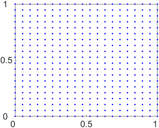
(a) Uniform sequence

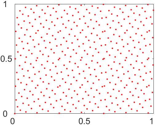
(b) Hammersley sequence

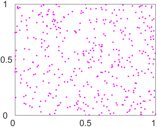
(c) Random sequence

Figure 3.1: Uniform sequence (a), Hammersley sequence (b) and random sequence (c) for discretizing target distribution.

Let us formulate the “discrete” reflector antenna problem. We consider the target distribution $\mu_{t}$ given by (1.3) has an approximate form of

$$\mu_{t}^{K}(z)=\sum_{i=1}^{K}\pi_{i}\delta(z-z_{i}),$$ (3.1)

which is expressed as the sum of Dirac measures $\delta$, where $\mathcal{P}=\{z_{1},z_{2},\dots,z_{K}\}$ is a series of points on the target domain $\Omega$ and $\pi_{i}=\pi(z_{i})$. In this section, the selection of the point set $\mathcal{P}$ on the target domain must adhere to the principle of approximating the target distribution with the fewest number of points. This requirement arises from the fact that the efficiency of the supporting paraboloid method depends on the number of points in that set. In [60], the authors simply defined the point set $\mathcal{P}$ by uniformly dividing the target domain, which results in exponential growth of the number of points in this set with respect to the dimension of the target distribution. In this paper, we propose a point set on the target domain that does not depend on the dimension of the target distribution, specifically low-discrepancy sequences (Hammersley sequence) and random sequences (see Figure 3.1). It is easy to see that the number of points in a uniform sequence will grows exponentially with respect to the target distribution dimension, whereas the number of points in a Hammersley sequence or random sequence can remains constant. Therefore, we obtain a dimensionality-independent approach for constructing the reflecting surface. We recommend using uniform sequences for low-dimensional target distributions and, conversely, opting for low-discrepancy sequences or random sequences in higher dimensions. Since the reflector antenna system is on sphere, we transform (3.1) to the unit sphere, that is, $\mu_{O}$ given by (1.4) is approximated as

$$\mu_{O}^{K}(y)=\sum_{i=1}^{K}g_{i}\delta(y-y_{i}),\quad y\in\Omega_{O},$$ (3.2)

where $g_{i}=\pi\circ Q(y_{i})$ and $y_{i}=Q^{-1}(z_{i}),z_{i}\in\mathcal{P}$. The “discrete” version of the reflector antenna problem consists of constructing a reflecting surface $R_{K}$ given by (2.1), i.e., the union of a series of pieces of paraboloids of revolution with common focus origin and axial directions $\{y_{1},y_{2},\dots,y_{K}\}$, that the rays from a source are reflected in directions $\{y_{1},y_{2},\dots,y_{K}\}$ such that the total energy in each direction $y_{i}$ equals $g_{i}$. For each $y_{i}$, the (2.4) can be rewritten as

$$\mu_{R_{K}}(y_{i})=\int_{V(y_{i})}f(x)\,\mathrm{d}\sigma(x),$$ (3.3)

which is the amount of energy sent by the reflecting surface $R_{K}$ in the direction $y_{i}$, where $V(y_{i})$ is the visibility set of all rays reflected by the $R_{K}$ in the direction $y_{i}$. The discrete reflector antenna problem is to determine a reflecting surface $R_{K}$, defined by (2.1) (i.e., paraboloids $\{P(y_{1}),\dots,P(y_{K})\}$), that satisfies

$$\mu_{O}^{K}(y_{i})=\mu_{R_{K}}(y_{i}),\quad i=1,2,\dots,K,$$

that is

$$g_{i}=\mu_{R_{K}}(y_{i}),\quad i=1,2,\dots,K,$$ (3.4)

which is a discrete form of (2.5). It was shown that if the energy conservation condition

$$\int_{\Omega_{I}}f(x)\,\mathrm{d}\sigma(x)=\sum_{i=1}^{K}g_{i},$$ (3.5)

i.e., (1.6) holds, then one can construct in a finite number of steps a reflecting surface $R_{K}$ such that

$$\sum_{i=1}^{K}(\mu_{R_{K}}(y_{i})-g_{i})^{2}\leq\epsilon.$$ (3.6)

for any prescribed in advance number $\epsilon>0$ in [8]. The conservation of energy, i.e., (3.5) is easily satisfied by normalizing (3.2).

In the following, we briefly describe the supporting paraboloid method proposed in [8] for finding an approximate solution of (3.4) that satisfies (3.6). Let us fix $\epsilon>0$, positive integer $K>1$ and the point $y_{i}\in\Omega_{O},i=1,2,\dots,K$ (or $z_{i}\in\Omega,i=1,2,\dots,K$). A reflecting surface $R_{K}$ is completely determined by the vector $(d_{1},d_{2},\dots,d_{K})$. Thus we identify a reflecting surface $R_{K}$ with a $(d_{1},d_{2},\dots,d_{K})$. Let $\mathcal{R}$ be the class of reflecting surfaces $R_{K}=(d_{1},d_{2},\dots,d_{K})$ with a fixed $d_{1}$ such that

$$\mu_{R_{K}}(y_{i})\leq g_{i}+\frac{\epsilon}{\sqrt{K(K-1)}}.$$ (3.7)

This is always possible since

$$\mu_{R_{K}}(y_{i})\to 0,\quad\text{as all}\;\;d_{2},d_{3},\dots,d_{K}\to+\infty,$$

for each $i=1,2,\dots,K$, which means that $\mu_{R_{K}}(y_{i})$ is monotonic with respect to $d_{i}$ [8]. We can use the monotonicity of $\mu_{R_{K}}$ to construct a series of reflecting surfaces in the set $\mathcal{R}$ and it converges to a solution of (3.4). The implementation of the supporting paraboloid method can be initialized with any reflecting surface in $\mathcal{R}$. In the following numerical experiments, the initial reflecting surface is given by

$$R_{K}^{0}=(d_{1},\alpha d_{2},\dots,\alpha d_{K})$$ (3.8)

where $\alpha>1$. Obviously $R_{K}^{0}\in\mathcal{R}$. Suppose that the $j$-th element $R_{K}^{j}$ of the sequence of reflecting surfaces is constructed. To build the $R_{K}^{j+1}$ from $R_{K}^{j}$, we iteratively scale focal parameters $d_{i}$ of each paraboloid of $R_{K}^{j}$ until the desired target distribution is produced. By repeating the entire scaling process over, we can obtain a sequence of reflecting surfaces $\{R_{K}^{1},R_{K}^{2},\dots\}$ which ultimately converges to a solution of (3.4) that achieves the desired density at each point $y_{i}$. The steps of the supporting paraboloid method are summarized in Algorithm 1 [8, 32, 60].

Algorithm 1 Construct reflecting surfaces by enhanced supporting paraboloid method

1:Target points $\{z_{i}\in\Omega,i=1,2,\dots,K\}$, error $\epsilon>0$, transformation $Q$, source density $f$ on $\Omega_{I}$ and target density $\pi$ on $\Omega$

2:A sequence of reflectors $\{R_{K}^{1},R_{K}^{2},\dots\}$

3:Use the transformation $Q$ to convert $z_{i}$ to $y_{i}$ on $\Omega_{O}$, i.e., $y_{i}=Q^{-1}(z_{i})$

4:Choose an initial reflector $R_{K}^{0}=(d_{1}^{0},d_{2}^{0},\dots,d_{K}^{0})\in\mathcal{R}$, given by (3.8)

5:Initialize $\widetilde{R}=R_{K}^{0}$, $j=0$ and increments $\Delta d=(0,0,\dots,0)$

6:Compute measured distribution $\mu_{\widetilde{R}}=(\mu_{\widetilde{R}}(y_{1}),\mu_{\widetilde{R}}(y_{2}),\dots,\mu_{\widetilde{R}}(y_{K}))$

7:while $\mu_{\widetilde{R}}$ does not satisfy the condition (3.6) do

8:     Let $J\subset\{2,3,\dots,K\}$ be the subset of indices for which $\mu_{\widetilde{R}}(y_{i})$ do not satisfy (3.7)

9:     if $J$ is a empty then

10:         $R_{K}^{j+1}=\widetilde{R}$ and $\Delta d_{i}=d_{i}^{j}/3,\;i\in\{2,3,\dots,K\}$

11:     else

12:         $R_{K}^{j+1}=R_{K}^{j}$ and $\Delta d_{i}=\Delta d_{i}/2,\;i\in J$ 

13:     end if

14:     Put $\widetilde{R}=R_{K}^{j+1}-\Delta d=(d_{1}^{j+1},d_{2}^{j+1}-\Delta d_{2},\dots,d_{K}^{j+1}-\Delta d_{K})$

15:     Evaluate the measured distribution $\mu_{\widetilde{R}}=(\mu_{\widetilde{R}}(y_{1}),\mu_{\widetilde{R}}(y_{2}),\dots,\mu_{\widetilde{R}}(y_{K}))$ and set $j=j+1$

16:end while

Remark 3.1.

1. In order to satisfy the energy conservation condition (3.5), let $g_{i}=\beta g_{i}$ where $\beta=\int_{\Omega_{I}}f(x)\,\mathrm{d}\sigma(x)/\sum_{i=1}^{K}g_{i}$ or $f=\beta^{\prime}f$ where $\beta^{\prime}=\sum_{i=1}^{K}g_{i}/\int_{\Omega_{I}}f(x)\,\mathrm{d}\sigma(x)$. Algorithm 1 can produce a class of convex reflecting surfaces that converge to a solution of (3.4). If one desires a concave reflecting surface, the negative increments must be instead of positive increments in line $12$ of Algorithm 1. This algorithm is similar to the supporting ellipsoid method in [33, 60], except that the ellipsoid is replaced by the paraboloid, which is mainly caused by the difference between near field and far field.

2. Algorithm 1 is easy to implement. We only iterate the focal parameter of the paraboloid, which does not depend on the dimension of the reflector antenna problem. Low-discrepancy sequences or random sequences are used to discretize the target distribution; thus, the algorithm is dimension-independent. Furthermore, it can be seen that the target distribution only needs to be computed $K$ times at input and not again during the entire iteration, which is a huge advantage for sampling complex target distributions, especially in PDEs-constrained Bayesian inverse problems. In addition, the algorithm does not require gradient information regarding the density of the target distribution, making it gradient-free.

3. In [8], the authors proved the convergence of the algorithm. This algorithm is based on an iterative procedure and does not require an initial guess, which is automatically generated by the algorithm. However, the algorithm exhibits only a linear rate of convergence. Given a desired error $\epsilon$, this algorithm constructs in $K^{2}/\epsilon$ steps a reflecting surface such that the difference between $g_{i}$ and the amount of rays actually received in the direction $y_{i}$ is bounded by $\epsilon$ for every $i=1,2,\dots,K$, that is, satisfying the (3.6). Notice that the convergence in this paper is dimension-independent due to the application of low-discrepancy sequences or random sequences in discretizing target distributions. There has been some work on improving the supporting paraboloid algorithms, including iterative methods based on the Nelder-Mead algorithm [32], Newton’s method [21], and techniques for quickly calculating the intersections of paraboloids [15]. However, we emphasize that this paper does not focus on efficiently solving the reflector design problem.

In Algorithm 1, the measure $\mu_{R_{K}}$ defined by equation (3.3) must be evaluated multiple times during each iteration. The speed of the algorithm and the accuracy of the results are significantly influenced by the efficiency of the $\mu_{R_{K}}$ evaluation method. Given a set of paraboloids, we need to determine how much energy is collected by each paraboloid. Computing the exact intersections between paraboloids is a challenging and resource-intensive operation. Instead, we employ Monte Carlo ray tracing to evaluate the measure $\mu_{R_{K}}$ [55, 21, 60]. The general idea is to trace a set of rays through the system and collect the rays on a direction $y_{i}$. Let $X:=\{x_{j},j=1,2\dots,N\}$ is the sample points (i.e., unit directions or rays) distributed by source density $f$ on the $\Omega_{I}$. Then the source measure $\mu_{I}$ given by (2.6) has the discrete form

$$\mu_{I}^{N}(x)=\sum_{i=1}^{N}f_{i}\delta(x-x_{i}),\quad x\in\Omega_{I},$$ (3.9)

where $f_{i}=f(x_{i})$, and the energy conservation condition (3.5) can be rewritten as

$$\sum_{i=1}^{N}f_{i}=\sum_{i=1}^{K}g_{i}.$$

The the measure $\mu_{R_{K}}$ on the direction $y_{i}$ is estimated by [60]

$$\mu_{R_{K}}(y_{i})=\frac{\mathcal{S}(\Omega_{I})}{N}\sum_{j=1}^{N_{i}}f(x_{ij}),$$

where $\{x_{ij},j=1,2\dots,N_{i}\}$ is the number of those rays emitted from $V(y_{i})$ and $X=\sum_{i=1}^{K}\sum_{j=1}^{N_{i}}x_{ij}$, and $\mathcal{S}(\Omega_{I})$ denotes the area of $\Omega_{I}$. In order to obtain $\{x_{ij},j=1,2\dots,N_{i}\}$, we need to check whether every ray in $X$ is emitted from $V(y_{i})$. In our case, we only require to determine the supporting paraboloid for each ray $x_{j},j=1,2\dots,N$. If a given ray is reflected by a paraboloid $P(y_{i})$, we know without further calculation that the ray will be reflected to its axial direction $y_{i}$. If a reflecting surface is given by (2.1), then the supporting paraboloid $P(y_{i})$ that reflects the ray $x_{j}$ is the one closest to the source, namely

$$i=\operatorname*{arg\,min}_{k}p_{y_{k},d(y_{k})}(x_{j}),\quad k\in\{1,2,\dots,K\}.$$ (3.10)

It is evident that tracing more rays (i.e., larger number $N$) provides a better estimate of the measure $\mu_{R_{K}}$. The statistical error associated with Monte Carlo ray tracing is given by $N_{i}^{-1/2}$ for the estimation of $\mu_{R_{K}}(y_{i})$, which is independent of the dimensionality. The iterative process in Algorithm 1 should be terminated as soon as the output values of $\mu_{R_{K}}$ fall below the peak statistical error, as measurements at this point are dominated by statistical noise.

3.2 Dual re-simulation

Our goal is to generate samples from the target distribution using a reflector antenna system. Given a reflecting surface obtained through the enhanced supporting paraboloid method, how can we use it to generate the desired samples? Possible approaches include directly utilizing reflection mapping and stereographic projection, as described in equation (1.5), or re-simulating the reflection antenna system via ray tracing. However, the reflecting surface produced by the enhanced supporting paraboloid method serves as the inner envelope of a series of paraboloids, as defined in equation (2.1). Consequently, while it is continuous, slope discontinuities occur at the edges of each patch of paraboloids. If we re-simulate the reflector antenna system or utilize the mapping in (1.5), we encounter two issues: firstly, multiple rays from the source will be reflected by the patches of supporting paraboloids in the same direction, namely in the direction of their axes; secondly, rays will be reflected by the edges of the patches of supporting paraboloids in the incorrect direction. In [60, 21], the authors produce a smooth reflecting surface by interpolating the polar radius or focal parameters of the paraboloids. For standard Cartesian or structured meshes in low-dimensional spaces, this is not problematic, as there are many various interpolation techniques that have been well-studied. Our discrete target distribution on the contrary is based on including not only the structured meshes but also the unstructured low-discrepancy sequences or random sequences in high-dimensional space. Therefore, to address the aforementioned problems during sampling from the target distribution using the reflector antenna system, we propose a dual re-simulation method based on dual reflector antennas in this section.

Figure 3.2: The dual reflector antenna system

Let $R_{\rho}$ be a convex reflecting surface. The Legendre transform of $\rho$ with respect to the $1/(1-x\cdot y),x\in\Omega_{I},y\in\Omega_{O}$ is a function $\rho^{\ast}$ defined on $S^{n}$, given by

$$\rho^{\ast}(y)=\inf_{x\in\Omega_{I}}\frac{1}{\rho(x)(1-x\cdot y)}.$$ (3.11)

Lemma 3.1.

Given a convex reflecting surface $R_{\rho(x)},x\in\Omega_{I}$ and let a function $\rho^{\ast}(y),y\in\Omega_{O}$ defined by (3.11) be the Legendre transform of $\rho$. Then $y=T_{\rho}(x)$ if and only if $x=T_{\rho^{\ast}}(y)$ almost everywhere, where $x\in\Omega_{I},y\in\Omega_{O}$, $T_{\rho}$ and $T_{\rho^{\ast}}$ are the subdifferential given by Definition 2.3 with respect to $\rho$ and $\rho^{\ast}$, respectively.

The derivation for this lemma has been given in [65]. To ensure the coherence and completeness of the paper, we provide this proof.

Proof.

For any fixed $y_{0}\in\Omega_{O}$, let the infimum (3.1) be attained at $x_{0}\in\Omega_{I}$. Then

$$\rho^{\ast}(y_{0})=\frac{1}{\rho(x_{0})(1-x_{0}\cdot y_{0})}.$$ (3.12)

For any $x\neq x_{0}$ in $\Omega_{I}$ and from (3.1), we have

$$\rho(x)\leq\frac{1}{\rho^{\ast}(y_{0})(1-x\cdot y_{0})},\quad x\in\Omega_{I}.$$ (3.13)

From (3.12) and (3.13), we see that $p_{y_{0},d}(x)=d/(1-x\cdot y_{0}),d=1/\rho^{\ast}(y_{0})$ is a supporting paraboloid of $\rho$ at $x_{0}$. Due to the symmetry between $x$ and $y$, we get

$$\rho^{\ast}(y)\leq\frac{1}{\rho(x_{0})(1-x_{0}\cdot y)},\quad y\in\Omega_{O}.$$ (3.14)

It follows from (3.12) and (3.14) that $p_{x_{0},d^{\ast}}(x)=d^{\ast}/(1-x_{0}\cdot y),d^{\ast}=1/\rho(x_{0})$ is a supporting paraboloid of $\rho^{\ast}$ at $y_{0}$. Thus we complete the proof. ∎

Remark 3.2.

Obviously, for a convex reflecting surface $R_{\rho}$ and its Legendre transform $\rho^{\ast}$, we have $d(y)=1/\rho^{\ast}(y),y\in\Omega_{O}$ and $d^{\ast}(x)=1/\rho(x),x\in\Omega_{I}$. In particular the Legendre transform of $\rho^{\ast}$ is $\rho$ itself, i.e., $\rho^{\ast\ast}=\rho$. Moreover, if $\rho$ is smooth, then $T_{\rho^{\ast}}$ is the inverse of $T_{\rho}$, i.e., $T_{\rho^{\ast}}=T_{\rho}^{-1}$. And if the reflecting surface is a solution of reflector antenna problem, that is, $\rho$ satisfies (1.7), then $\rho^{\ast}$ satisfies the equation

$$\mathcal{A}\rho^{\ast}(y)=\frac{g(y)}{f\circ T_{\rho_{\ast}}(y)},\quad y\in\Omega_{O},$$

where $\mathcal{A}$ is the operator in (1.7), and the radial graph

$$R_{\rho^{\ast}}=\{y\rho^{\ast}(y):\rho^{\ast}>0,y\in\Omega_{O}\},$$

called the dual reflecting surface, is a solution of the dual of the reflector antenna problem (see Figure 3.2).

Corollary 3.2.

Let $R_{\rho(x)},x\in\Omega_{I}$ be a convex reflecting surface and its polar radius is given by (2.2). For any ray $x\in\Omega_{I}$ from source (i.e., sample distributed by $\mu_{I}$), then the direction in which it is reflected by this reflecting surface $R_{\rho}$, i.e., the push-forward of the sample, is given by

$$y=T_{\rho}(x)=\arg\inf_{y\in\Omega_{O}}\frac{d(y)}{1-x\cdot y},\quad d(y)=\frac{1}{\rho^{\ast}(y)},$$ (3.15)

and the pull-back of $y$ is given by

$$x=T_{\rho^{\ast}}(y)=\arg\inf_{x\in\Omega_{I}}\frac{d^{\ast}(x)}{1-x\cdot y},\quad d^{\ast}(x)=\frac{1}{\rho(x)},$$ (3.16)

where $\rho^{\ast}$ is the Legendre transform of $\rho$.

Remark 3.3 (re-simulating or ray tracing).

A reflecting surface reflects the ray $x$ (resp. $y$) in the direction $T_{\rho}(x)$ (resp. $T_{\rho^{\ast}}(y)$). The procedure described above is referred to as re-simulating or ray tracing the reflector system (resp. dual reflector system), and this constitutes a sampling of $\mu_{R_{\rho}}=(T_{\rho})_{\sharp}\mu_{I}$ (resp. $\mu_{R_{\rho^{\ast}}}=(T_{\rho^{\ast}})_{\sharp}\mu_{O}$).

Given a fixed target point set $\mathcal{P}=\{z_{i},i=1,\dots,K:z_{i}\in\Omega\}$, we denote $\mathcal{P}_{O}=\{y_{i},i=1,\dots,K:y_{i}=Q^{-1}(z_{i})\in\Omega_{O}\}$. From (2.2), the polar radius of a reflecting surface $R_{K}=(d_{1},d_{2},\dots,d_{K})$ obtained by the Algorithm 1 is given by

$$\hat{\rho}(x)=\min_{y_{i}\in\mathcal{P}_{O}}\frac{d_{i}}{1-x\cdot y_{i}},\quad x\in\Omega_{I}.$$

As discussed above, the reflecting surface $R_{\hat{\rho}}=\{x\hat{\rho}(x):x\in\Omega_{I}\}$ is the envelope of $K$ paraboloids with axis direction $y_{i}\in\mathcal{P}_{O}$, and it is continuous but its derivatives is discontinuous, that is, the surface is $C^{0}$ continuity. If a new sample point $x^{\prime}$ from the distribution of the light source goes to re-simulate this reflector system, from (3.15) we get the push-forward of this sample as

$$y_{j}=T_{\hat{\rho}}(x^{\prime})=\operatorname*{arg\,min}_{y_{i}\in\mathcal{P}_{O}}\frac{d_{i}}{1-x^{\prime}\cdot y_{i}},$$ (3.17)

which is also the direction in which it is reflected by the reflecting surface $R_{\hat{\rho}}$, as well as a sample from approximate geometric optics approximation measure. It is clear that the direction is not the desired one, as $y_{j}\in\mathcal{P}_{O}$ is a fixed point. In fact, if we can obtain an ideal and smooth reflecting surface $R_{\rho}$, the exact push-forward of this sample $x^{\prime}$ should lie within a small domain containing $y_{j}$; that is, $T_{\rho}(x^{\prime})\in U(y_{j})$ where $U(x)$ denotes a small domain containing $x$. Furthermore, as $K\to\infty$ in the supporting paraboloid method, we have $T_{\hat{\rho}}(x^{\prime})=T_{\rho}(x^{\prime})$, which means that the $U(y_{j})$ is reduced to a single point. Despite identifying a smaller domain, we still face challenges in determining exactly which point corresponds to $T_{\rho}(x^{\prime})$. However, given a point $y^{\prime}$ in $U(y_{j})$, we can ascertain whether it corresponds to $T_{\rho}(x^{\prime})$ based on the dual reflecting surface. Next, we present a dual re-simulation method based on Lemma 3.1.

Let $X=\{x_{j},j=1,\dots,N\}$ denote the rays used to ray-trace the reflector antenna system. By (3.10), for each $y_{i}\in\mathcal{P}_{O}$, we can obtain the rays $\{x_{ij},j=1,\dots,N_{i}\}$ that are reflected by the supporting paraboloid $P(y_{i})$. The rays $X$ are divided into $K$ parts, each corresponding to a supporting paraboloid. We take the mean of each parts, denoted as

$$x_{i}=\frac{1}{N_{i}}\sum_{j=1}^{N_{i}}x_{ij}$$

as the ray corresponding to the axial direction of the supporting paraboloid $P(y_{i})$, i.e., $y_{i}=T_{\hat{\rho}}(x_{i})$, and the mean of polar radius of each parts, denoted as

$$\rho_{i}=\frac{1}{N_{i}}\sum_{j=1}^{N_{i}}\hat{\rho}(x_{ij})$$

as the polar radius corresponding to $x_{i}$. From Lemma 3.1 and the equation $y_{i}=T_{\hat{\rho}}(x_{i})$, we have $x_{i}=T_{\hat{\rho}^{\ast}}(y_{i})$, where $\hat{\rho}^{\ast}$ is the polar radius of the dual reflecting surface $R_{\hat{\rho}}$ given by

$$\hat{\rho}^{\ast}(y)=\min_{x_{i}\in\mathcal{P}_{I}}\frac{d^{\ast}_{i}}{1-x_{i}\cdot y},\quad y\in\Omega_{O},$$

where $\mathcal{P}_{I}=\{x_{1},x_{2},\dots,x_{K}\}$ and $d^{\ast}_{i}=1/\rho_{i}$. Analogous to reflecting surface $R_{\hat{\rho}}$, the dual reflecting surface $R_{\hat{\rho}^{\ast}}=\{y\hat{\rho}^{\ast}(y):y\in\Omega_{O}\}$ is also the envelope of $K$ paraboloids with axis direction $x_{i}\in\mathcal{P}_{I}$, and exhibits $C^{0}$ continuity. Given a sample point $y^{\prime}$ from the distribution of the output light intensity on $\Omega_{O}$ (i.e., $\mu_{O}$), let it to re-simulate this dual reflector system. From (3.16) we get the push-forward of $y^{\prime}$, which represents the direction in which it is reflected by this dual reflecting surface $R_{\hat{\rho}^{\ast}}$, as

$$x_{k}=T_{\hat{\rho}^{\ast}}(y^{\prime})=\operatorname*{arg\,min}_{x_{i}\in\mathcal{P}_{I}}\frac{d^{\ast}_{i}}{1-x_{i}\cdot y^{\prime}}.$$ (3.18)

This direction is clearly not our desired one, since $x_{k}\in\mathcal{P}_{I}$ is a fixed point. If the dual reflecting surface is smooth, the exact push-forward of $y^{\prime}$ lies within a small domain containing $x_{k}$; that is, $T_{\rho^{\ast}}(y^{\prime})\in U(x_{k})$. If $k=j$, then $p_{y_{j},d_{j}}$ is the supporting paraboloid of $R_{\hat{\rho}}$ at $x_{k}$ and $p_{x_{k},d^{\ast}_{k}}$ is the supporting paraboloid of $R_{\hat{\rho}^{\ast}}$ at $y_{j}$. We set $T_{\hat{\rho}}(x^{\prime})=y^{\prime}$, which is reasonable. For the reflecting surface $R_{\hat{\rho}}$, we cannot determine the exact direction in which $x^{\prime}$ is reflected by; we can only state that the direction of reflection lies within a small domain that contains $y_{j}$. Similarly, for its dual reflecting surface $R_{\hat{\rho}^{\ast}}$, we cannot specify the exact direction in which $y^{\prime}$ is reflected; we can only assert that the direction of reflection lies within a small domain containing $x_{k}$. However, if $y_{j}$ and $x_{k}$ are mutual the axial direction of the supporting paraboloid, then we can conclude that $T_{\hat{\rho}}(x^{\prime})=y^{\prime}$ and $T_{\hat{\rho}^{\ast}}(y^{\prime})=x^{\prime}$. Thus, we need only find a $y^{\prime}$ such that the axial direction $x_{k}$ of the supporting paraboloid of its dual reflecting surface at point $y^{\prime}\hat{\rho}^{\ast}(y^{\prime})$ corresponds to the axial direction $y_{k}$ of the supporting paraboloid of reflecting surface at point $x^{\prime}\hat{\rho}(x^{\prime})$. We refer to this process as dual re-simulation or dual ray tracing, and its steps are summarized in Algorithm 2.

Algorithm 2 Dual re-simulating the reflector antenna system

1:A reflecting surface $R_{K}=(d_{1},d_{2},\dots,d_{K})$ given by Algorithm 1, point set $\mathcal{P}_{O}=\{y_{1},\dots,y_{K}\}$ and $\mathcal{P}_{I}=\{x_{1},\dots,x_{K}\}$

2:Samples $\{y_{1}^{\prime},y_{2}^{\prime},\dots,y_{M}^{\prime}\}$ from output measure $\mu_{O}$ on $\Omega_{O}$

3:for all $i=1,2,\dots,M$ do

4:     Draw a sample (i.e., ray) $x_{i}^{\prime}$ from source measure $\mu_{I}$ on $\Omega_{I}$

5:     Compute $y_{j}=T_{\hat{\rho}}(x_{i}^{\prime})$ using (3.17)

6:     Set $k=0$

7:     while $j\neq k$ do

8:         Given a candidate point $\tilde{y}$ from $U(y_{j})$

9:         Compute $x_{k}=T_{\hat{\rho}^{\ast}}(\tilde{y})$ using (3.18)

10:     end while

11:     $y_{i}^{\prime}=\tilde{y}$

12:end for

Remark 3.4.

In step $6$ of Algorithm 2, we first transform $y_{j}$ onto the target domain $\Omega$, then draw $\tilde{y}^{\prime}$ from a distribution with a support set containing the point $Q^{-1}(y_{j})$, and finally transform $\tilde{y}^{\prime}$ onto the domain $\Omega_{O}$, i.e.,

1. Compute $y_{j}^{\prime}=Q^{-1}(y_{j})$;

2. Sample $\tilde{y}^{\prime}$ from a distribution $\mu_{j}$ with support set containing the point $y_{j}^{\prime}$;

3. Compute $\tilde{y}=Q(\tilde{y}^{\prime})$;

where the distribution $\mu_{j}$ can be set to a Gaussian distribution with $y_{j}^{\prime}$ as the mean, a uniform distribution centered on $y_{j}^{\prime}$, or other similar distributions. This distribution $\mu_{j}$ is selected based on the criterion that the union of all support of $\mu_{j},j=1,\dots,K$ covers $\Omega$, i.e.,

$$\Omega\subset\bigcup_{j=1}^{K}\operatorname{supp}(q_{j}-\epsilon),$$

where $q_{j}$ is the density of $\mu_{j}$, since we are sampling the target distribution over $\Omega$. The $\mu_{j}$ will only affect the speed of steps $5$ through $8$ in Algorithm 2 and not the drawn sample points themselves. In Section 5, for all numerical experiments, we take $\mu_{j}$ to be uniform distribution $\mathcal{U}(y_{j}^{\prime}-l/2\mathbf{1},y_{j}^{\prime}+l/2\mathbf{1})$ or Gaussian distribution $\mathcal{N}(y_{j}^{\prime},(l/6)^{2}I)$, where $\mathbf{1}=(1,1,\dots,1)$ and

$$l=\biggl{(}\frac{\mathcal{S}(\tilde{\Omega})}{K}\biggr{)}^{\frac{1}{n}}$$ (3.19)

depends on the area of the approximate target domain, the number of target points $K$ and dimension of the target distribution $n$, which represents the side lengths of the target domain divided equally into $K$ blocks. Certainly, we can choose other distributions as well. We emphasize that the selection of $\mu_{j}$ is not critical and is relatively insensitive.

Note that the dual re-simulation generates samples on the sphere, and transforming these samples to the target domain yields our desired samples from the target distribution. By combining the construction of reflecting surfaces with dual re-simulation, we summarize the geometric optics approximation sampling (GOAS) method proposed in this paper as follows:

 

Geometric optics approximation sampling (GOAS):

 

step1 (Offline)

computing a $C^{0}$ reflecting surface using the support paraboloid method, i.e., Algorithm 1;

step2 (Online)

obtaining samples from the output distribution on the sphere by dual re-simulating this reflector antenna system, i.e., Algorithm 2;

step3

using $Q$ to transform the samples given by step$2$ onto the target domain .

 

4 Error estimation under Wasserstein metrics

In the reflector antenna problem, only trivial analytical solutions, such as the spheres or a parabola (Dirac target measure), are known. The reflecting surface given by supporting paraboloid method in Section 3.1 is the convex hull of the interior intersections of a series of supporting paraboloids. This surface is $C^{0}$ and is approximated in comparison to a smooth ideal reflecting surface. On the other hand, from the sampling point of view, the primary concern is not the shape of reflector itself, but rather the quality of the dual re-simulation. As mentioned in Section 3.2, this dual re-simulation mathematically represents a sampling of the push-forward of source distribution or numerical geometric optics approximation measure. Therefore, in order to build an error estimation, we will consider the difference between the projection of the numerical geometric optics approximation measure onto target domain and the target measure. For this we will use the standard Wasserstein distance to measure the difference between distributions on the sphere [62, 63, 4].

Definition 4.1 (Wasserstein distances).

Given two compact manifold $\mathcal{X}$ and $\mathcal{Y}$ endowed with a continuous, bounded from below cost function $c(x,y):\mathcal{X}\times\mathcal{Y}\to\mathbb{R}$ for transporting one unit of mass from $x$ to $y$. Let $\mu_{1}$ and $\mu_{2}$ be measures on $\mathcal{X}$, $\mathcal{Y}$ respectively, the optimal transportation cost between $\mu_{1}$ and $\mu_{2}$ is defined by

$$OT_{c}(\mu_{1},\mu_{2})=\inf_{\gamma\in\Gamma(\mu_{1},\mu_{2})}\int_{\mathcal{X}\times\mathcal{Y}}c(x,y)\,\mathrm{d}\gamma(x,y)$$ (4.1)

where $\Gamma(\mu_{1},\mu_{2})$ is the set of measures $\gamma$ on $\mathcal{X}\times\mathcal{Y}$, called couplings of $\mu_{1}$ and $\mu_{2}$, satisfying $\gamma(A\times\mathcal{Y})=\mu_{1}(A)$ and $\gamma(\mathcal{X}\times B)=\mu_{2}(B)$ for all Borel subsets $A\subset\mathcal{X}$ and $B\subset\mathcal{Y}$. In particular, if $\mathcal{X}=\mathcal{Y}$ and $(\mathcal{X},d_{\mathcal{X}})$ is a compact metric space, then for $p\in[1,\infty]$, the Wasserstein distance of order $p$ between $\mu_{1}$ and $\mu_{2}$ is defined as $W_{p}(\mu_{1},\mu_{2})=(OT_{c}(\mu_{1},\mu_{2}))^{\frac{1}{p}}$ with

$$c(x,y)=\frac{1}{p}d^{p}_{\mathcal{X}}(x,y),\quad x,y\in\mathcal{X}.$$

Remark 4.1.

Given a measure $\gamma\in\Gamma(\mu_{1},\mu_{2})$ and pair of location $(x,y)$, the value of $\gamma(x,y)$ tells us what proportion of mass of $\mu_{1}$ at $x$ ought to be transferred to $y$ in order to reconfigure $\mu_{1}$ into $\mu_{2}$. In this section, the metric on the sphere is taken as

$$d_{S^{n}}(x,y)=\arccos(x\cdot y),$$ (4.2)

which denotes the geodesic distance between $x$ and $y$ on $S^{n}$.

In our setting of a complete separable metric space $\mathcal{X}$, one can represent $\gamma$ as a collection of conditional distributions $\{\gamma_{x}\}_{x\in\mathcal{X}}$ on $\mathcal{Y}$, in the sense that $\,\mathrm{d}\gamma(x,y)=\,\mathrm{d}\gamma_{x}(y)\,\mathrm{d}\mu_{1}(x)$. In fact, $W^{p}_{p}$ define the well-known Kantorovich’s formulation of optimal transport, which is a relaxation of the Monge problem, because for each transport map $T:\mathcal{X}\to\mathcal{Y}$ one can associate a transference plan $\gamma=\gamma_{T}$ of the same total cost [62, 63]. Let conditional distribution $\gamma_{x}=\delta(y-T(x))$ and it is seen that $\gamma(A\times B)=\mu_{1}(A\cap T^{-1}(B))$ and $\mu_{2}(B)=\mu_{1}(T^{-1}(B))$. Then

$$\int_{\mathcal{X}\times\mathcal{Y}}c(x,y)\,\mathrm{d}\gamma(x,y)=\int_{\mathcal{X}}\int_{\mathcal{Y}}c(x,y)\delta(y-T(x))\,\mathrm{d}y\,\mathrm{d}\mu_{1}(x)=\int_{\mathcal{X}}c(x,T(x))\,\mathrm{d}\mu_{1}(x).$$

It follows that

$$W^{p}_{p}(\mu_{1},\mu_{2})\leq\int_{\mathcal{X}}c(x,T(x))\,\mathrm{d}\mu_{1}(x).$$ (4.3)

It can be shown that

$$W^{p}_{p}(\mu_{1},\mu_{2})=\sup_{(\psi_{1},\psi_{2})}\biggl{\{}\int_{\mathcal{X}}\psi_{1}(x)\,\mathrm{d}\mu_{1}(x)-\int_{\mathcal{Y}}\psi_{2}(y)\,\mathrm{d}\mu_{2}(y)\biggr{\}},$$

where $(\psi_{1},\psi_{2})\in L^{1}(\mathcal{X})\times L^{1}(\mathcal{Y})$ and $\psi_{1}(x)+\psi_{2}(y)\leq c(x,y)$. This is called the dual formulation of Kantorovich [62, 63]. In special case where $p=1$ and $\mathcal{X}=\mathcal{Y}$ we have the very simple representation

$$W_{1}(\mu_{1},\mu_{2})=\sup\biggl{\{}\int_{\mathcal{Y}}\psi\,\mathrm{d}\mu_{1}(y)-\int_{\mathcal{Y}}\psi\,\mathrm{d}\mu_{2}(y)\bigg{|}\psi\in C^{0}(\mathcal{Y}),\|\psi\|_{Lip}\leq 1\biggr{\}}$$ (4.4)

where

$$\|\psi\|_{Lip}=\sup_{x\neq y}\frac{|\psi(x)-\psi(y)|}{c(x,y)}.$$

Theorem 4.1.

Let the output domain $\Omega_{O}\subset S^{n}$ and the compact target domain on a plane in $\Omega\subset\mathbb{R}^{n+1}$, and a diffeomorphism $Q$ transforms $\Omega_{O}$ to $\Omega$. The target measure $\mu_{t}$ on $\Omega$ is given by (1.3) and its discrete or approximate form $\mu_{t}^{K}$ is obtained by (3.1). The output rays distribution $\mu_{O}$ on $\Omega_{O}$ is given by (1.4) and its discrete or approximate form $\mu_{O}^{K}$ is obtained by (3.2). Then

$$W_{p}(\mu_{O},\mu_{O}^{K})\leq C_{2}p^{-1/p}\arccos(1-\frac{1}{2}C_{1}l^{2})$$

where positive parameters $C_{1}$ and $C_{2}$ depends on $Q$ and target measure $\mu_{t}$, respectively. And positive parameter $l$ depends only on target domain $\Omega$.

Proof.

Let $\mathcal{P}=\{z_{i}\}_{i=1}^{K}$ be a consequence on $\Omega$. Consider the Voronoi tessellations and let

$$U(z_{i}):=\{z\in\Omega:|z-z_{i}|\leq|z-z_{j}|,\text{for any}\;j\neq i\}$$

be the Voronoi cell for $z_{i}$. We choose some open balls $B_{l_{i}}(z_{i})$ with radius $l_{i}$,

$$l_{i}=\max_{z\in U(z_{i})}|z_{i}-z|,$$

centered at $z_{i}$. Then we have $U(z_{i})\subset B_{l_{i}}(z_{i})$ for all $i\in\{1,2,\dots,K\}$ and thus $\Omega\subset\cup_{i=1}^{K}B_{l_{i}}(z_{i})$. Define the map $F:\Omega\to\mathcal{P}$ such that $F(z)=z_{i}$ for all $z\in U(z_{i})$. Let $l=\max_{i\in\{1,2,\dots,K\}}l_{i}$, and obviously we have

$$|F(z)-z|\leq l$$ (4.5)

almost everywhere in $\Omega$. It can be easily check that this map $F$ is well-defined, since the intersection between $U(z_{i})$ and $U(z_{j})$ for $i\neq j$ is of zero Lebesgue measure and $\cup_{i=1}^{K}U(z_{i})=\Omega$. Thus $F$ is a transport map from $\mu_{t}$ to $\mu_{t}^{K}$, and then $F^{\prime}:=Q^{-1}\circ F\circ Q$ is a transport map from $\mu_{O}$ to $\mu_{O}^{K}$. Therefore, from (4.3) and (4.2), we have

$$W_{p}(\mu_{O},\mu_{O}^{K})\leq\biggl{(}\int_{\Omega_{O}}\frac{1}{p}\arccos^{p}(y\cdot F^{\prime}(y))\,\mathrm{d}\mu_{O}(y)\biggr{)}^{1/p}.$$ (4.6)

It follows from the formula $|x-y|^{2}=2(1-x\cdot y)$ for any $x,y\in S^{n}$ that

$$y\cdot F^{\prime}(y)=1-\frac{1}{2}|y-F^{\prime}(y)|^{2}=1-\frac{1}{2}|y-Q^{-1}\circ F\circ Q(y)|^{2}.$$

Then, by the change of variables formula, we have

$$\int_{\Omega_{O}}\frac{1}{p}\arccos^{p}(y\cdot F^{\prime}(y))\,\mathrm{d}\mu_{O}(y)=\int_{\Omega}\frac{1}{p}\arccos^{p}(1-\frac{1}{2}|Q^{-1}(z)-Q^{-1}\circ F(z)|^{2})\,\mathrm{d}\mu_{t}(z).$$ (4.7)

Since the $Q$ is a diffeomorphism, and by the (4.5), we have

$$|Q^{-1}(z)-Q^{-1}\circ F(z)|\leq C_{1}|z-F(z)|\leq C_{1}l.$$ (4.8)

Substituting (4.8) and (4.7) into (4.6), we get

$$W_{p}(\mu_{O},\mu_{O}^{K}) \leq\biggl{(}\int_{\Omega}\frac{1}{p}\arccos^{p}(1-\frac{1}{2}C_{1}l^{2})\,\mathrm{d}\mu_{t}(z)\biggr{)}^{1/p}$$

$$\leq C_{2}p^{-1/p}\arccos(1-\frac{1}{2}C_{1}l^{2}),$$

which completes the proof. ∎

Remark 4.2.

From the proof of the theorem, we know that the error bound for the output distribution is dependent on the set of points in its discrete form, i.e., $\mathcal{P}$. If the number $K$ of points in this set tends to infinity, we have $l\to 0$. Consequently, we obtain $W_{p}(\mu_{O},\mu_{O}^{K})=0$.

Theorem 4.2.

Let the input domain $\Omega_{I}\subset S^{n}$. The output rays distribution $\mu_{I}$ on $\Omega_{I}$ is given by (2.6) and its discrete or approximate form $\mu_{I}^{N}$ is obtained by (3.9). Then

$$W_{p}(\mu_{I},\mu_{I}^{N})\leq C_{2}p^{-1/p}\arccos(1-\frac{1}{2}C_{1}r^{2})$$

where $C_{1},C_{2}$ and $r$ are positive parameters.

Remark 4.3.

Theorem 4.2 tells us that the discrete error bound for the source distribution depends on the number of ray traced when constructing the reflecting surface. If the number $N$ of ray traced tends to infinity, we have $r\to 0$. Obviously, we obtain $W_{p}(\mu_{I},\mu_{I}^{N})=0$.

Similar to the error bound for the output distribution, the proof of Theorem 4.2 can be found in Appendix A.

Lemma 4.3.

Let $\mathcal{M}_{1}$ and $\mathcal{M}_{2}$ be two compact manifold in $\mathbb{R}^{n+1}$ endowed with two geodesic distance $d_{\mathcal{M}_{1}}$ and $d_{\mathcal{M}_{2}}$, respectively. Let the $\mu_{1}$ and $\mu_{2}$ be two measures on the manifold $\mathcal{M}_{1}$. If the map $T:\mathcal{M}_{1}\to\mathcal{M}_{2}$ is Lipschitz continuous, then

$$W_{p}(T_{\sharp}\mu_{1},T_{\sharp}\mu_{2})\leq LW_{p}(\mu_{1},\mu_{2}),$$

where $L$ is the Lipschitz constant of $T$.

Proof.

Let $\gamma\in\Gamma(u_{1},u_{2})$, and define a measure

$$\gamma_{T}:=(T\times T)_{\sharp}\gamma,$$

which is a coupling of $T_{\sharp}u_{1}$ and $T_{\sharp}u_{2}$, i.e., $\gamma_{T}(B\times C)=\gamma(T^{-1}(B)\times T^{-1}(C))$ for any Borel set $B,C\subset\mathcal{M}_{2}$. Then

$$W_{p}(T_{\sharp}u_{1},T_{\sharp}u_{2}) =\biggl{(}\inf_{\gamma_{T}\in\Gamma(T_{\sharp}u_{1},T_{\sharp}u_{2})}\int_{\mathcal{M}_{2}\times\mathcal{M}_{2}}\frac{1}{p}d^{p}_{\mathcal{M}_{2}}(x,y)\,\mathrm{d}\gamma_{T}(x,y)\biggr{)}^{1/p}$$

$$\leq\biggl{(}\int_{\mathcal{M}_{2}\times\mathcal{M}_{2}}\frac{1}{p}d^{p}_{\mathcal{M}_{2}}(x,y)\,\mathrm{d}\gamma_{T}(x,y)\biggr{)}^{1/p}$$

$$=\biggl{(}\int_{\mathcal{M}_{1}\times\mathcal{M}_{1}}\frac{1}{p}d^{p}_{\mathcal{M}_{2}}(T(x),T(y))\,\mathrm{d}\gamma(x,y)\biggr{)}^{1/p}.$$ (4.9)

Since the map $T:\mathcal{M}_{1}\to\mathcal{M}_{2}$ is Lipschitz continuous, we have

$$d^{p}_{\mathcal{M}_{2}}(T(x),T(y))\leq L^{p}d^{p}_{\mathcal{M}_{1}}(x,y),$$

where $L$ is the Lipschitz constant of $T$. Plugging this bound into (4), we deduce that

$$W_{p}(T_{\sharp}u_{1},T_{\sharp}u_{2})\leq\biggl{(}\int_{\mathcal{M}_{1}\times\mathcal{M}_{1}}\frac{1}{p}L^{p}d^{p}_{\mathcal{M}_{1}}(x,y)\,\mathrm{d}\gamma(x,y)\biggr{)}^{1/p},$$

which implies

$$W_{p}(T_{\sharp}\mu_{1},T_{\sharp}\mu_{2})\leq LW_{p}(\mu_{1},\mu_{2}).$$

∎

Lemma 4.4.

Let the output domain $\Omega_{O}\subset S^{n}$ be bounded and $\mu_{1},\mu_{2}$ be two measures on $\Omega_{O}$. For every $p\in[1,+\infty]$, then

$$W^{p}_{p}(\mu_{1},\mu_{2})\leq CW_{1}(\mu_{1},\mu_{2}),$$

where positive constant $C$ depends only on $\Omega_{O}$ and $p$.

Proof.

If $\Omega_{O}$ is bounded, then for any $x,y\in\Omega_{O}$

$$d^{p}_{S^{n}}(x,y)\leq(\max_{x_{1},y_{1}\in\Omega_{O}}d^{p-1}_{S^{n}}(x_{1},y_{1}))d_{S^{n}}(x,y)=(\text{diam}(\Omega_{O}))^{p-1}d_{S^{n}}(x,y),$$

where $\text{diam}(\Omega_{O})$ denotes the diameter of the domain $\Omega_{O}$. Hence,

$$W^{p}_{p}(\mu_{1},\mu_{2}) =\inf_{\gamma\in\Gamma(u_{1},u_{2})}\int_{\Omega_{O}\times\Omega_{O}}\frac{1}{p}d^{p}_{S^{n}}(x,y)\,\mathrm{d}\gamma(x,y)$$

$$\leq\int_{\Omega_{O}\times\Omega_{O}}\frac{1}{p}d^{p}_{S^{n}}(x,y)\,\mathrm{d}\gamma(x,y)$$

$$\leq(\text{diam}(\Omega_{O}))^{p-1}\int_{\Omega_{O}\times\Omega_{O}}\frac{1}{p}d_{S^{n}}(x,y)\,\mathrm{d}\gamma(x,y),$$

which yields $W^{p}_{p}(\mu_{1},\mu_{2})\leq\text{diam}^{p-1}(\Omega_{O})W_{1}(\mu_{1},\mu_{2})$. ∎

From the perspective of optimal transportation, a straightforward evaluation of the supporting paraboloid method would be to build an approximate transport map; that is, we obtain an inaccurate reflecting map $T_{\hat{\rho}}$ where $\hat{\rho}$ is the polar radius of the reflecting surface $R_{K}$. Therefore we provide an error estimate for this reflecting map in the discrete case.

Theorem 4.5.

Let $\hat{\rho}$ be the polar radius of a reflecting surface $R_{K}=(d_{1},d_{2},\dots,d_{K})$ given by Algorithm 1, and let the reflecting map $\widetilde{T}=T_{\hat{\rho}}$. The discrete forms of input distribution on $\Omega_{I}$ and output distribution on $\Omega_{O}$, i.e., $\mu_{I}^{N}$ and $\mu_{O}^{K}$, are given by (3.9) and (3.2), respectively. Then

$$W_{p}^{p}(\widetilde{T}_{\sharp}\mu^{N}_{I},\mu_{O}^{K})\leq C\epsilon,$$

where positive constant $C$ depends only on $\Omega_{O}$ and $p$. And $\epsilon>0$ is any prescribed in advance error bound in (3.6).

Proof.

By the Lemma 4.4, we have

$$W_{p}^{p}(\widetilde{T}_{\sharp}\mu^{N}_{I},\mu_{O}^{K})\leq C_{1}W_{1}(\widetilde{T}_{\sharp}\mu^{N}_{I},\mu_{O}^{K}),$$ (4.10)

where the positive constant $C_{1}$ depends on $\Omega_{O}$ and $p$. From (4.4), we have

$$W_{1}(\widetilde{T}_{\sharp}\mu^{N}_{I},\mu_{O}^{K})=\sup\biggl{\{}\int_{\Omega_{O}}\psi\,\mathrm{d}(\widetilde{T}_{\sharp}\mu^{N}_{I}-\mu_{O}^{K})(y)\bigg{|}\psi\in C^{0}(\Omega_{O}),\|\psi\|_{Lip}\leq 1\biggr{\}}.$$ (4.11)

If the geodesic distance $d_{S^{n}}$ is bounded by some constant $C_{2}$, then from (4.11) we have

$$W_{1}(\widetilde{T}_{\sharp}\mu^{N}_{I},\mu_{O}^{K})\leq C_{2}\sup\biggl{\{}\int_{\Omega_{O}}\psi\,\mathrm{d}(\widetilde{T}_{\sharp}\mu^{N}_{I}-\mu_{O}^{K})(y)\bigg{|}\text{continuous}\;\psi:\Omega_{O}\to[-1,1]\biggr{\}}.$$

Hence, we have

$$W_{1}(\widetilde{T}_{\sharp}\mu^{N}_{I},\mu_{O}^{K}) \leq C_{2}\int_{\Omega_{O}}\,\mathrm{d}(\widetilde{T}_{\sharp}\mu^{N}_{I}-\mu_{O}^{K})(y)$$

$$\leq C_{2}\sum_{i=i}^{K}|\mu_{R_{K}}(y_{i})-\mu_{O}^{K}(y_{i})|$$

$$\leq C_{2}\sum_{i=i}^{K}(\mu_{R_{K}}(y_{i})-g_{i})^{2}$$

$$\leq C_{2}\epsilon,$$

where the last inequality follows from (3.6). Combining this with (4.10) completes the proof.

∎

Theorem 4.6.

Let the bounded output domain $\Omega_{O}\subset S^{n}$ and the compact target domain $\Omega$ on a plane in $\mathbb{R}^{n+1}$, and a diffeomorphism $Q$ transforms $\Omega_{O}$ to $\Omega$. The source distribution on the input domain $\Omega_{I}\subset S^{n}$ and target measure on $\Omega$, i.e., $\mu_{I}$ and $\mu_{t}$, are given by (2.6) and (1.3), respectively. Let $\widetilde{T}=T_{\hat{\rho}}$ where $\hat{\rho}$ is the polar radius of a reflecting surface $R_{K}=(d_{1},d_{2},\dots,d_{K})$ given by Algorithm 1. Then

$$W_{p}((Q\circ\widetilde{T})_{\sharp}\mu_{I},\mu_{t})\leq C_{1}\arccos(1-\frac{1}{2}C_{2}r^{2})+C_{3}\epsilon^{1/p}+C_{4}\arccos(1-\frac{1}{2}C_{5}l^{2}),$$

where $C_{i},i=1,\dots,5$ are the positive constants. The positive constants $r$ and $l$ are depend only on the $\Omega_{I}$ and $\Omega$, respectively. And the $\epsilon>0$ is the error bound in (3.6).

Proof.

Let $B\subset\Omega$ and observe that $\widetilde{T}^{-1}(Q^{-1}(B))=(Q\circ\widetilde{T})^{-1}(B)$. Then

$$(Q\circ\widetilde{T})_{\sharp}\mu_{I}(B)=\mu_{I}((Q\circ\widetilde{T})^{-1}(B))=\mu_{I}(\widetilde{T}^{-1}(Q^{-1}(B)))=\widetilde{T}_{\sharp}\mu_{I}(Q^{-1}(B))=Q_{\sharp}(\widetilde{T}_{\sharp}\mu_{I})(B).$$

The $Q:\Omega_{O}\to\Omega$ is a diffeomorphism, then $Q_{\sharp}\mu_{O}=\mu_{t}$. Thus from Lemma 4.3 we have

$$W_{p}((Q\circ\widetilde{T})_{\sharp}\mu_{I},\mu_{t}) =W_{p}(Q_{\sharp}(\widetilde{T}_{\sharp}\mu_{I}),Q_{\sharp}\mu_{O})$$

$$\leq C_{1}W_{p}(\widetilde{T}_{\sharp}\mu_{I},\mu_{O}).$$

By the triangle inequality and Lemma 4.3, we have

$$W_{p}(\widetilde{T}_{\sharp}\mu_{I},\mu_{O}) \leq W_{p}(\widetilde{T}_{\sharp}\mu_{I},\widetilde{T}_{\sharp}\mu_{I}^{N})+W_{p}(\widetilde{T}_{\sharp}\mu_{I}^{N},\mu_{O})$$

$$\leq C_{2}W_{p}(\mu_{I},\mu_{I}^{N})+W_{p}(\widetilde{T}_{\sharp}\mu_{I}^{N},\mu_{O})$$

$$\leq C_{2}W_{p}(\mu_{I},\mu_{I}^{N})+W_{p}(\widetilde{T}_{\sharp}\mu_{I}^{N},\mu_{O}^{K})+W_{p}(\mu_{O}^{K},\mu_{O}).$$

Hence, from Theorem 4.1, Theorem 4.2 and Theorem 4.5, we complete this proof. ∎

Remark 4.4.

Theorem 4.6 provides an error estimate between the projection of the geometric optics approximation measure onto the target domain and the target distribution. It is easy to see that the error bound consists of three terms: a discrete error in the ray tracing of the source distribution, an error in the propagation of the discrete error in the target measure to the output distribution, and a computational error in the process of constructing the reflecting surface. Obviously, if both the number of ray traced and the number of discrete sequence points in the target measure tend to infinity, then the first two error terms will vanish. Further, if the error $\epsilon$ in (3.6) is set to $0$, we can obtain the exact reflecting surface, leading to $(Q\circ\widetilde{T})_{\sharp}\mu_{I}=\mu_{t}$.

5 Numerical experiments

Several numerical experiments are presented in this section to characterize the performance of geometric optics approximation sampling (GOAS). We compare the method with the traditional Markov chain Monte Carlo (MCMCs) simulations and the sampling via measure transport map (TM), respectively. Moreover, we use geometric optics approximate sampling to solve three inverse scattering problems: locating acoustic sources, inverse scattering from an open arc and simultaneous reconstruction of multiple parameters in a nonlinear advection-diffusion-reaction model. In these numerical experiments, different sequences–specifically, low-discrepancy sequences and random sequences–are used to obtain the target points for discretizing the target distribution in our approach. By analyzing these numerical experiments, we can gain insight into the performance and applicability of geometric optics approximation sampling in various situations. Additionally, it also confirms the theoretical results for error estimate.

In Algorithm 1, we set $\epsilon=10^{-4}$. Let $y=(y_{1},y_{2},\dots,y_{n+1})\in\mathbb{R}^{n+1}$ and $z=(z_{1},z_{2},\dots,z_{n})\in\mathbb{R}^{n}$. We set the transformation $Q$ to a stereographic projection, i.e.,

$$Q(y_{1},y_{2},\dots,y_{n+1})=\frac{(y_{1},y_{2},\dots,y_{n})}{1-y_{n+1}}$$

and its inverse

$$Q^{-1}(z_{1},z_{2},\dots,z_{n})=\frac{(2z_{1},2z_{2},\dots,2z_{n},|z|-1)}{|z|+1}.$$

Both maps are continuous and thus $Q:S^{n}\setminus\{(0,0,\dots,1)\}\to\mathbb{R}^{n}$ is a diffeomorphism. Furthermore, for all numerical experiments, we take the source distribution to be uniform in the north hemisphere. The rays $x$ from the source distribution is generated by normalizing the sample points from a standard Gaussian distribution, i.e.,

$$x=\frac{X}{|X|},\quad X\sim\mathcal{N}(0,I),$$

where $I$ is the identity matrix in $\mathbb{R}^{n+1}$.

5.1 GOAS vs. MCMCs for strongly non-Gaussian distributions

In this section, we compare the performance of our geometric optics approximation sampler (GOAS) with that of several existing MCMC methods, including the Metropolis-Hasting (MH) [52], slice sampler [44], Hamiltonian Monte Carlo (HMC) [16, 43] and the Metropolis-Adjusted Langevin Algorithm (MALA) [53]. For a comprehensive comparison, we consider the models based on several two-dimensional synthetic datasets: Funnel, Banana, Mixture of Gaussians (MoG), Ring, and Cosine [66, 29]. Together, these non-Gaussian distributions encompass a range of geometric complexities and multimodality.

In this numerical experiment, we use the Hammersley sequence to obtain a discrete representation of all non-Gaussian distributions within GOAS method. The true densities and kernel density estimations obtained through various methods are visualized in Figure 5.1, where the rightmost column of the figure displays the computational time in seconds and the number of model evaluations (i.e., density evaluations) provided by GOAS and MCMC simulations with respect to the effective sample size (ESS), refer to Appendix B for details of its computation. Obviously, compared to the MCMCs method, our GOAS approach captures the boundaries of all strongly non-Gaussian distributions more clearly. The slice sampler also produces good density estimates, including those for the Mixture of Gaussians. However, the computational time and number of model evaluations for slice sampling, as well as other MCMC simulations, are proportional to the effective sample size. In contrast, our GOAS method does not depend on ESS. Therefore, when a large number of samples need to be drawn from complex distributions, our GOAS method can be significantly more efficient then traditional MCMC simulation techniques, especially for Bayesian inverse problems governed by partial differential equations.

5.2 GOAS vs. Transport Maps

In this section, we compare the performance of our geometric optics approximation sampling (GOAS) method and Transport Maps (TM) in addressing different problems. Our GOAS method does not require the gradients of the posterior density, whereas TM does. We consider two simple Bayesian inference problems: the Biochemical Oxygen Demand (BOD) model [59, 41] and the Euler-Bernoulli beam problem [49]. For details on the Bayesian inverse problem framework, refer to Appendix B. The BOD problem has a closed-form posterior distribution, allowing the gradients of its density to be easily obtained, while the posterior distribution for the Euler-Bernoulli beam Bayesian inverse problem is constrained by a differential equation, with the gradients of its density computed using finite differences. In addition, to ensure a fair comparison of the performance of our GOAS method and TM, the BOD problem has the same geometric structure of the posterior distribution as the Euler Bernoulli beam problem. For the computation of TM, we refer to the literature [3, 48].

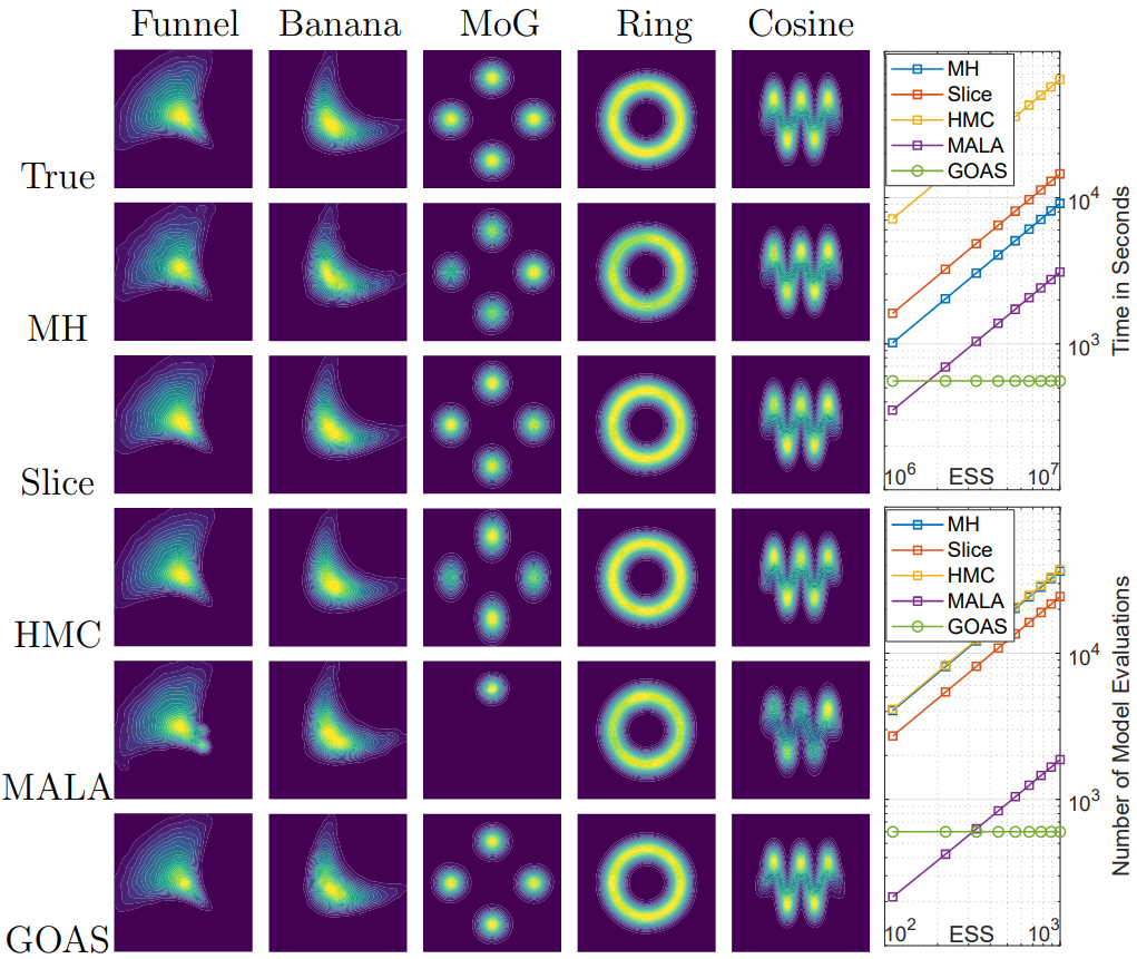
Figure 5.1: Comparison of GOAS and MCMCs for non-Gaussian distribution sampling. True densities and the kernel density estimations obtained from the GOAS and MCMCs simulation (the first five columns), as well as the computational time in seconds and number of model evaluations provided by different methods regarding the ESS (the sixth column) for sampling the MoG distribution.

Biochemical Oxygen Demand Model

For the Biochemical Oxygen Demand (BOD) problem, the objective is to estimate two coefficients in a time-dependent model of oxygen demand, which serves as an indicator of biological activity in a water sample. The simple time-dependent forward model is given by

$$\mathcal{G}(t)=A(1-\exp(-Bt)),$$

where $A=[0.4+0.4(1+erf(\theta_{1}/\sqrt{2}))]$ and $B=[0.01+0.15(1+erf(\theta_{2}/\sqrt{2}))]$. The measurement data is obtained by $y(t)=\mathcal{G}(t)+\eta$ where $\eta\sim\mathcal{N}(0,10^{-3})$. The objective is to characterize the posterior density of parameters $\theta=(\theta_{1},\theta_{2})$ knowing observation of the system at time $t={1,2,3,4,5}$, i.e., $y=(y(1),y(2),y(3),y(4),y(5))=(0.18,0.32,0.42,0.49,0.54)$. Using a standard Gaussian prior for parameters $\theta$ and from equation (B.3), the posterior density is given by

$$\pi(\theta)=\exp\biggl{[}-\frac{1}{2}\frac{1}{10^{-3}}\sum_{i=1}^{5}(\mathcal{G}(t_{i})-y(t_{i}))^{2}-\frac{1}{2}\theta\theta^{T}\biggr{]}.$$

Obviously, it is easy to obtain the gradients of the posterior density.

Euler Bernoulli beam problem

Consider a cantilever beam of $L>0$ length modeled by the $\Omega=[0,L]$, and the left boundary is fixed at the origin and the right boundary is free. The Euler-Bernoulli beam is governed by the fourth-order differential equation

$$\frac{\partial^{2}}{\partial x^{2}}\biggl{(}E(x)\frac{\partial^{2}}{\partial x^{2}}u(x)\biggr{)}=f(x),\quad x\in\Omega,$$ (5.1)

where $u:\Omega\to\mathbb{R}$ is the vertical deflection of the beam and $f:\Omega\to\mathbb{R}$ is the load. The effective stiffness of the beam is given by $E:\Omega\to\mathbb{R}$ describes beam geometry and material properties. We consider a smoothed piecewise constant approximation $\widetilde{E}_{2}:\Omega\times\mathbb{R}\to\mathbb{R}$ of the stiffness $E$ that depends on parameters $\theta=(\theta_{1},\theta_{2})$. The forward operator $\mathcal{G}$ is then given by numerically solving (5.1) with stiffness $\widetilde{E}_{2}$. The Euler Bernoulli beam problem is to infer the parameters $\theta$ in $\widetilde{E}_{2}$ from the measurements of displacement $u$ in $\Omega$. In order to compare the effects of the different problems on the GOAS and TM methods, we set the appropriate parameters to achieve a consistent geometric structure of the posterior distribution, specifically the “banana shape”. For details on the inverse problem setup, refer to Appendix C.

(a)

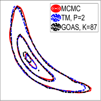
(b)

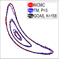
(c)

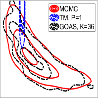
(d)

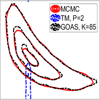
(e)

(f)

Figure 5.2: Kernel density estimations using $5\times 10^{3}$ samples obtained by GOAS with the increasing number of parabolas $K$ and TM with Hermite polynomials degree $P=1,\;P=2,\;P=3$ for Biochemical Oxygen Demand model (a)-(c) and Euler Bernoulli beam problem (d)-(f). The estimates of the MCMC simulation, i.e., the red line, serves as the “true” density.

Table 5.1: The sample Mean, Variance, Skewness and Kurtosis of $\theta=(\theta_{1},\theta_{2})$ given by different methods for Biochemical Oxygen Demand model and Euler Bernoulli Beam problem.

Method		Mean	Variance	Skewness	Kurtosis
Biochemical Oxygen Demand model
MCMC “true”		(0.0340, 0.9224)	(0.1443, 0.3716)	(1.781, 0.6741)	(7.329, 3.440)
TM	P=1	(0.0921, 0.9682)	(0.0289, 0.1155)	(-0.0040, -0.0654)	(2.884, 2.926)
	P=2	(0.0328, 0.9111)	(0.1264, 0.4004)	(1.609, 1.156)	(7.373, 5.784 )
	P=3	(0.0383, 0.9147)	(0.1611, 0.3831)	(2.737, 0.9659)	(20.88, 5.115)
	K=35	(0.0609, 0.8384)	(0.1697, 0.3715)	(1.858, 0.8179)	(8.213, 3.611)
	K=87	(0.0467, 0.9014)	(0.1509, 0.3854)	(1.810, 0.6721)	(7.901, 3.296)
GOAS	K=158	(0.0459, 0.9302)	(0.1704, 0.4019)	(1.919, 0.5989)	(7.853, 3.184)
Euler Bernoulli Beam Problem
MCMC “true”		(0.7316, 1.397)	(0.0338, 0.1025)	(1.126, 0.6622)	(4.498, 3.310)
TM	P=1	(0.5793, 3.410)	(0.0001, 1.040)	(0.0079, -0.0060)	(3.053, 3.057)
	P=2	(0.6584, 1.755)	(0.0000, 0.2013)	(-11.31, 0.5504)	(217.2, 5.807)
	P=3	(0.7204, 1.423)	(0.0365, 0.1090)	(1.797, 0.5487)	(9.847, 3.146)
	K=36	(0.7218, 1.403)	(0.0321, 0.1144)	(1.219, 0.5752)	(5.135, 2.902)
	K=85	(0.7314, 1.407)	(0.0346, 0.1062)	(1.165, 0.6730)	(4.673, 3.232)
GOAS	K=158	(0.7303, 1.405)	(0.0344, 0.1066)	(1.159, 0.7187)	(4.672, 3.437)

Table 5.2: Computational time (s and h denote seconds and hours, respectively) and the number of forward model evaluations required by GOAS with $K=158$ and TM with $P=3$ methods for Biochemical Oxygen Demand model and Euler Bernoulli Beam problem at the same ESS.

Method	Offline		Online time (s)	Total (h)
	model evaluation	time (s)
Biochemical Oxygen Demand model
TM, P=3	$7.7\times 10^{5}$	6.902	0.0213	0.0019
GOAS, K=158	$1.16\times 10^{4}$	165.4	0.0653	0.0459
Euler Bernoulli Beam Problem
TM, P=3	$9.48\times 10^{6}$	$9.8078\times 10^{4}$	0.4096	27.24
GOAS, K=158	$1.1\times 10^{4}$	157.5	0.0808	0.0437

Comparison results

For our GOAS method, we first need to identify the target domain $\Omega$, and then use the Hammersley sequence within $\Omega$ to discretize the posterior distribution. In this example, $10^{4}$ samples from the prior distribution are used to detect the domain $\Omega$ where the posterior density values exceed $\epsilon$. For the TM method, we employ the total-order Hermite polynomials of degree $P=1,2,3$, and use second-order central differences to approximate the gradient of the posterior density for the Euler Bernoulli beam problem. All runtime measurements were implemented using Matlab on a single core computer node equipped with an Inter Core i7-4790 processor and 16-GB RAM.

The kernel density estimations given by GOAS with $K=35,87,158$ and TM with $P=1,2,3$ for BOD model and Euler Bernoulli beam problem are shown in Figure 5.2. The results from MCMC method serve as the “true” density. Clearly, geometric structure of the posterior distribution of the BOD model is consistent with that of the Euler Bernoulli beam problem. The density estimates from our method GOAS gradually converge to the true density as the number of parabolas $K$ increases for both the BOD model and the Euler Bernoulli beam problem. Furthermore, the increment in the number of parabolas $K$ is the same for both problems, which suggests that the performance of method GOAS is forward problem-independent and depends only on the geometric structure of the posterior distribution. However, with the same degree increasing, the density estimates from the TM method can progressively approach the posterior density of the BOD model but do not align closely with the posterior density of the Euler Bernoulli beam problem. Referring to the second row of Figure 5.2, the TM method does not work at $P=1,P=2$. The TM method may require higher degree Hermite polynomials to accurately fit the posterior density of the Euler Bernoulli beam problem. Thus, the performance of the TM method may depends not only on the geometric structure of the distribution but also on the specific forward problem being addressed. The reason our method GOAS is forward problem-independent is that it requires only the discretization of the posterior distribution over the $\Omega$ domain, whereas the TM method needs to iteratively compute both the posterior density and its gradient during optimization. Table 5.1 lists the first four sample moments obtained by GOAS with $K=35,87,158$ and TM with $P=1,2,3$ for BOD model and the Euler Bernoulli beam problem. As the number of parabolas increases, the GOAS method yields better estimates of these moments for both problems, which is consistent with Figure 5.2. We can find that even with small number of parabolas, i.e., $K=35,36$, the GOAS method still captures the mean and variance, as shown in the seventh and fifteenth rows of Table 5.1. The TM method with cubic map yields good mean and variance but fails to accurately obtain higher order moments for the BOD model. The sample moments of the Euler-Bernoulli beam problem obtained using the TM method are completely inaccurate, except for the mean and variance at $P=3$, which is consistent with Figure 5.2.

Finally we compare the computational efficiency of GOAS and TM method. For both inverse problems, the computational time and the number of forward model evaluations required by GOAS with $K=158$ and TM with $P=3$ method, both achieving the same effective sample size, are listed in Table 5.2. It is evident that the GOAS and TM methods exhibit negligible online time, while their primary computational cost is incurred offline; specifically, the GOAS method constructs a reflecting surface, and the TM method optimizes a map. For the BOD models with closed form posterior density, it is clear that TM method is more than $20$ times faster than the GOAS method. However, for the Euler Bernoulli beam problem, our GOAS method is $623$ times faster than the TM method due to the fact that the TM method computes $9.469\times 10^{6}$ more forward problems than the GOAS method. For the BOD model, the TM method also computes $7.584\times 10^{5}$ more forward problems. The TM method requires iterative computation of the posterior density as well as its gradient, whereas GOAS only needs to compute the posterior density at a low-difference sequence. In addition, the number of forward problems evaluations for the TM method depends on the approximation of Kullback-Leibler (KL) divergence and the degree of Hermite polynomials. When implementing the TM method, a sample-average approximation (SAA) is commonly used to approximate KL divergence [18, 41, 3]. The better the approximation of KL divergence–e.g., by using more samples from the reference distribution for SAA or by increasing the degree of Hermite polynomials–the greater number of forward problems that need to be computed. For the Euler Bernoulli beam problem, if the TM method is to achieve the same density estimation accuracy as GOAS, it must increase the degree of Hermite polynomials, which in turn will require greater computational cost. Therefore, the GOAS method is generally more efficient than the TM method for Bayesian inverse problems constrained by differential equations. Moreover, for problems with analytic posterior densities, the efficiency of the GOAS method is acceptable.

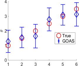
(a) Noise Level=10%

(b) Noise Level=5%

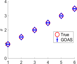
(c) Noise Level=1%

Figure 5.3: Sample mean and $95\%$ confidence interval of $\theta$ given by GOAS with $K\approx 800$ method at noise level:$10\%\,(a),\;5\%\,(b),\;1\%\,(c)$ for locating acoustic sources.

(a) low-discrepancy sequence

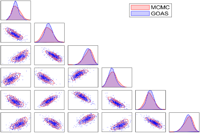
(b) random sequence

Figure 5.4: Sample points and marginal density estimates of $\theta$ given by GOAS with low-discrepancy sequence (a) and random sequence (b) at $5\%$ noise level for locating acoustic sources. The MCMC results serves as “true” values.

5.3 Locating acoustic sources

This examples is concerned with the inverse acoustic source problem from the far field measurements for the Helmholtz system. Consider the following Helmholtz equation

$$\Delta u^{s}+k^{2}u^{s}=S\quad\text{in}\ \mathbb{R}^{2},$$ (5.2)

where $k>0$ is the wave number, $u^{s}$ is the scattered field, and the source

$$S=\sum_{i=1}^{N}\lambda_{i}\delta_{z_{i}},$$ (5.3)

where $N$ is a positive integer, $z_{i}$ are points in $\Omega$ and $\lambda_{i}\neq 0$ are scalar quantities. By the asymptotic behavior of the fundamental solution to the Helmholtz equation, we can obtain the far field pattern. The locating acoustic source problem is to determine the locations $z_{i}$ from measurements of the far field pattern [38, 19, 17]. Refer to Appendix C for details on the inverse problem setup.

In this example, to discretize the posterior distribution, we first obtain a chain with length $3\times 10^{4}$ using MCMC simulation, and then cluster this chain into some classes using the K-means method [39]. The center points of the class with the posterior density values greater than $\epsilon$ are selected as the discrete points in the target domain $\Omega$. The set consisting of these center points can be viewed as a low-discrepancy sequence. Alternatively, we can first determine the $\Omega$ using a prior distribution or a short Markov chain, and then use the Hammersley sequence to obtain the discrete points for posterior density discretization.

Figure 5.3 shows sample mean and the $95\%$ confidence interval of $\theta=\{\theta_{i}\}_{i=1}^{6}$ obtained using GOAS method at $1\%,5\%,10\%$ noise level for the locating acoustic sources problem. As the noise level decreases, the sample means converge to the true values, and the confidence intervals gradually shrink, which indicates that our method GOAS is stable with respect to the noise level. Figure 5.4 illustrates the sample points and marginal density estimates of $\theta$ given by GOAS using a low-discrepancy sequence ($K=783$) and a random sequence ($K=707$) for discretizing the posterior density at a $5\%$ noise level, with the MCMC results considered as “true”. The random sequence consists of points generated from the Markov chains without clustering, taken five points apart, with posterior density values exceeding $\epsilon$. The results indicate that the low-discrepancy sequence provides a better fit than the random sequence, probably due to the smaller number of points in the random sequence compared to the low-discrepancy sequence. However, the sample points produced by the GOAS method using both sequence are mainly concentrated in regions of high probability, and the marginal density estimates given by these samples are consistent with the “true” marginal densities. This confirms that our approach is stable with respect to the target domain.

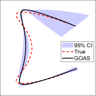
(a) Noise Level=10%

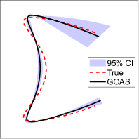
(b) Noise Level=5%

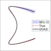
(c) Noise Level=1%

Figure 5.5: Sample mean and $95\%$ confidence interval (CI) of $\theta$ given by GOAS with $K\approx 890$ method at noise level:$10\%\,(a),\;5\%\,(b),\;1\%\,(c)$ for inverse scattering from an open arc.

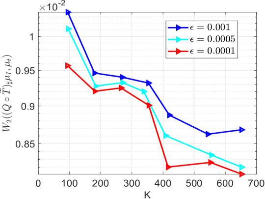
Figure 5.6: Wasserstein distance with $p=2$ between “true” posterior measure $\mu_{t}$ and projection of the numerical push-forward of source measure $\widetilde{T}_{\sharp}\mu_{I}$ where $\widetilde{T}=\widetilde{T}_{\hat{\rho}}$ and $\hat{\rho}$ is given by GOAS method at $\epsilon=0.001,0.0005,0.0001$ error bound in (3.6) with respect to $K$ for inverse scattering from an open arc.

5.4 Inverse scattering from an open arc

In this section, we consider the shape identification of open arc in scattering problem. The scattering of time-harmonic acoustic wave from thin obstacles lead to the scattering problem [36, 35]

$$(\Delta+k^{2})u =0,\quad\text{in}\;\mathbb{R}^{2}\setminus\Gamma$$ (5.4)

$$u =0,\quad\text{on}\;\Gamma$$ (5.5)

with wave number $k>0$ and the $\Gamma$ is a analytic arc in $\mathbb{R}^{2}$. The Dirichlet boundary condition corresponds to scattering from a sound-soft arc. The total field is $u=u^{i}+u^{s}$, where $u^{i}$ denotes the given incident field and the unknown scattered field $u^{s}$ satisfies the Sommerfeld radiation condition, i.e., (C.2). The inverse problem is to determine the shape of the arc $\Gamma$ from a konwledge of the far field pattern for the scattering of one incident plane wave. More details of the inverse problem can be found in Appendix C.

(a) True, $m_{d}$

(b) GOAS, $m_{d}$

(c) Std, $m_{d}$

(d) True, $m_{0}$

(e) GOAS, $m_{0}$

(f) Std, $m_{0}$

Figure 5.7: Posterior sample mean and sample standard deviation (Std) obtained via GOAS with $K=350$ for inferring the diffusion coefficient field $m_{d}$ (first row) and the initial condition field $m_{0}$ (second row) in a nonlinear advection-diffusion-reaction model.

Sample mean and $95\%$ confidence interval of $\theta$ given by GOAS method at $1\%,5\%,10\%$ noise level for inverse scattering from an open arc are shown in Figure 5.5. With the noise level decreasing, the sample means are close to the true and the confidence intervals gradually shrink, which indicate that our method GOAS is stable with respect to the noise level. Figure 5.6 plots the Wasserstein distance with $p=2$ between “true” posterior measure and projection of the numerical push-forward of source measure, i.e., $W_{2}(\widetilde{T}_{\sharp}\mu_{I},\mu_{t})$ where $\widetilde{T}=\widetilde{T}_{\hat{\rho}}$ and $\hat{\rho}$ is given by our GOAS method at $\epsilon=0.001,0.0005,0.0001$ error bound in (3.6), with respect to $K$ for this problem. The MCMC results are considered as “true” values. In this example, we approximate Wasserstein distances by adding an entropic regularization penalty to the original Kantorovich formulation of the optimal transport problem. The minimization of the regularized problem can be solved using a simple alternating minimization scheme, which involves iterations of straightforward matrix-vector products [50]. We tackle this problem using Sinkhorn algorithm with regularization parameter $0.001$. Obviously, as $K$ increases or $\epsilon$ decreases, the Wasserstein distance between posterior measure and the push-forward of source measure gradually decreases, which is consistent with the result stated in Theorem 4.6.

5.5 Simultaneous reconstruction of multiple parameters in a nonlinear advection-diffusion-reaction model

In this section, we deal with an inverse problem governed by a time-dependent advection-diffusion-reaction (ADR) model with a simple cubic reaction term. Our goal is to jointly infer the unknown diffusion coefficient field and the unknown initial condition field. We consider the advection-diffusion-reaction initial-boundary value problem

$$\frac{\partial u}{\partial t}+\nu\cdot\nabla u-\nabla\cdot(m_{d}\nabla u)+cu^{3} =f\quad\text{in}\;\Omega\times(0,T),$$ (5.6)

$$\frac{\partial u}{\partial v} =0\quad\text{on}\;\partial\Omega\times(0,T),$$ (5.7)

$$u|_{t=0} =m_{0}\quad\text{in}\;\Omega,$$ (5.8)

where $v$ is unit normal of $\partial\Omega$, and $m_{d}\in L^{2}(\Omega)$ and $m_{0}\in L^{2}(\Omega)$ are the diffusion coefficient and initial field, respectively. The parameter $\nu$ represents the advection velocity field, $c$ denotes the reaction coefficient, and $f$ is the source term. It is evident that the forward problem (5.6) is nonlinear. The inverse problem is to determine both the diffusion coefficient filed and initial condition field $(m_{d},m_{0})$ in ADR model using the measurements data $u(x,T),x\in\Omega$ [23]. More details about the inverse problem can be found in Appendix C.

The samples mean and standard deviation provided by GOAS for the inversion fields $(m_{d},m_{0})$ are shown in Figure 5.7. It can be observed that the initial condition field $m_{0}$ and the diffusion coefficient field $m_{d}$ estimated by GOAS with $K=350$ are very close to the true field, and both achieve a small sample standard deviation. Additionally, the inferred results fall within the $95\%$ confidence interval, as indicated by its sample standard deviation.

6 Conclusions

We have presented a novel sampling method, called geometric optics approximation sampling, to sample from challenging target measure. This sampler is based on the reflector antenna problem, which is concerned with constructing a reflecting surface such that rays from a source with a sampler distribution is reflected off to the output domain and creates a prescribed in advance light distribution. The key idea is to set the distribution on the output domain as a projection of the target measure on the sphere. Once a desired reflecting surface is obtained, one can draw an arbitrary number of independent and uncorrelated samples from target measure simply by dual re-simulating or rays tracing the reflector antenna system and then projecting the traced rays onto target domain. Therefore, the geometric optics approximation sampling approach consists of two main steps: the first step constructs a reflecting surface offline, and the second step dual re-simulation or ray tracing this reflector antenna system online, which in turn is then projected onto the target domain to obtain samples from the target measure. In the offline step, the reflector antenna problem is solved using the enhanced supporting paraboloid method, where the reflecting surface is defined as the convex hull of the interior intersections of a series of paraboloids and then the diameters of all the paraboloids are iteratively scaled until convergence is achieved to obtain the desired reflecting surface. The diameters of the paraboloids are obviously dimensionality-independent, and the gradient of density in the target distribution is not required during the iteration process. Notice that, for the supporting paraboloid method, we use low-discrepancy sequences or random sequences to discretize the target distribution. Since the reflector antenna problem is a optimal transportation problem, in the online step, we have proposed a dual re-simulating or rays tracing method based on its dual reflecting surface to generate samples from the target measure. This dual re-simulation can be applied to the discrete target measure not only on the uniform grids but also with low-discrepancy sequences and random sequences. For our method, we establish some theoretical analysis and error estimates. A geometric optics approximation measure, i.e., the push-forward of the source distribution, is defined by the reflecting surface. We show that this measure is well-defined. In particular, we give a result on the stability of this measure with respect to the target domain, which in turn ensures the numerical stability during sampling. Moreover, we derive a error estimate between the projection of the numerical geometric optics approximation measure and the target measure under the Wasserstein metrics, which consists of three error terms: the ray tracing error in the light source distribution, the discrete error in the target measure, and the computational error in the process of constructing the reflecting surface.

As has been demonstrated by the several examples and numerical experiments, the geometric optics approximation sampling is efficient, robust, and applicable. On the one hand, comparing with the traditional MCMC simulation, our sampler is more efficient and suitable for sampling a variety of strongly non-Gaussian complex distributions. On the other hand, comparing with other methods that require gradient information about the target density, such as measurable transport sampling, our approach is also efficient and stable because it do not depend on the forward problem itself but only on the geometric structure of the posterior measure, especially for Bayesian inverse problems constrained by partial differential equations. Moreover, our method can be applied to various Bayesian inverse problems. Finally, the numerical experiments confirm the theoretical results.

There are some potential extensions of this work. First, in this work, we use the Monte Carlo rays tracing to compute the actual output measure, which involves the computation of the intersection of the convex hull of confocal paraboloids in the supporting paraboloid method. One possible improvement is that this intersection can be computed as the intersection of a power diagram (a generalization of the Voronoi diagram) with the unit sphere [15]. Second, the reflector antenna problem can be framed as an optimal transportation problem, where its solution involves maximizing or minimizing a linear functional. Therefore we may use an efficient and stable algorithm in linear programming to solve the reflector antenna problem. Third, a fascinating extension of our current work is the application of geometric optics approximation sampling to accelerate Markov Chain Monte Carlo simulations. Finally, our method may be applied to sampling on manifolds, as well as to the construction of neural networks in deep learning. We plan to investigate these topics in the future.

Acknowledgment:  The work described in this paper was supported by the NSF of China (12271151) and NSF of Hunan (2020JJ4166) and Postgraduate Scientific Research Innovation Project of Hunan Province (CX20240364).

Appendix A Proof of Theorem 4.2

Proof.

Let a diffeomorphism $\alpha$ transform $\Omega_{I}$ to $\Sigma\subset\mathbb{R}^{n+1}$. From (2.6), we have

$$\mu_{s}(U)=\int_{U}f\circ\alpha^{-1}(z)\,\mathrm{d}\mu(z),\quad U\subset\Sigma,$$

which is a measure on $\Sigma$. Let $X=\{x_{i}\}_{i=1}^{N}$ be a rays consequence on $\Omega_{I}$. Similar to equation (3.9), we have the discrete form of $\mu_{s}$, i.e.,

$$\mu_{s}^{N}(z)=\sum_{i=1}^{N}t_{i}\delta(z-z_{i}),\quad z\in\Sigma,$$

where $z_{i}=\alpha(x_{i})$ and $t_{i}=f(x_{i})$. Consider the Voronoi tessellations and let

$$U(z_{i}):=\{z\in\Sigma||z-z_{i}|\leq|z-z_{j}|,\text{for any}\;j\neq i\}$$

be the Voronoi cell for $z_{i}$. We choose some open balls $B_{r_{i}}(z_{i})$ with radius $r_{i}$,

$$r_{i}=\max_{z\in U(z_{i})}|z_{i}-z|,$$

centered at $z_{i}$. Then we have $U(z_{i})\subset B_{r_{i}}(z_{i})$ for all $i\in\{1,2,\dots,N\}$ and thus $\Omega\subset\cup_{i=1}^{N}B_{r_{i}}(z_{i})$. Define the map $\beta:\Sigma\to\{\alpha(x_{i})\}_{i=1}^{N}$ such that $\beta(z)=z_{i}$ for all $z\in U(z_{i})$. Let $r=\max_{i\in\{1,2,\dots,N\}}r_{i}$, and obviously we have

$$|\beta(z)-z|\leq r$$ (A.1)

almost everywhere in $\Sigma$. It can be easily check that this map $\beta$ is well-defined, since the intersection between $U(z_{i})$ and $U(z_{j})$ for $i\neq j$ is of zero Lebesgue measure and $\cup_{i=1}^{N}U(z_{i})=\Sigma$. Thus $\beta$ is a transport map from $\mu_{s}$ to $\mu_{s}^{N}$, and then $\beta^{\prime}:=\alpha^{-1}\circ\beta\circ\alpha$ is a transport map from $\mu_{I}$ to $\mu_{I}^{N}$. Therefore

$$W_{p}(\mu_{I},\mu_{I}^{N}) \leq\biggl{(}\int_{\Omega_{I}}\frac{1}{p}\arccos^{p}(x\cdot\beta^{\prime}(x))\,\mathrm{d}\mu_{I}(x)\biggr{)}^{1/p}$$

$$=\biggl{(}\int_{\Omega_{I}}\frac{1}{p}\arccos^{p}(1-\frac{1}{2}|x-\beta^{\prime}(x)|^{2})\,\mathrm{d}\mu_{I}(x)\biggr{)}^{1/p}$$

$$=\biggl{(}\int_{\Sigma}\frac{1}{p}\arccos^{p}(1-\frac{1}{2}|\alpha^{-1}(z)-\alpha^{-1}\circ F(z)|^{2})\,\mathrm{d}\mu_{s}(z)\biggr{)}^{1/p}$$

$$\leq\biggl{(}\int_{\Sigma}\frac{1}{p}\arccos^{p}(1-\frac{1}{2}C_{1}|(z)-\alpha(z)|^{2})\,\mathrm{d}\mu_{s}(z)\biggr{)}^{1/p}$$

$$\leq\biggl{(}\int_{\Sigma}\frac{1}{p}\arccos^{p}(1-\frac{1}{2}C_{1}r^{2})\,\mathrm{d}\mu_{s}(z)\biggr{)}^{1/p}$$

$$\leq C_{2}p^{-1/p}\arccos(1-\frac{1}{2}C_{1}r^{2}),$$

where the first inequality follows from (4.3) and (4.2), the equality leading to the second line is an application of the formula $|x-y|^{2}=2(1-x\cdot y)$ for any $x,y\in S^{n}$, the third equality follows from the change of variables formula, and the fifth inequality follows from (A.1). ∎

Appendix B Bayesian inverse problem framework

Let $\mathbf{X}$ be a separable Hilbert space, equipped with the Borel $\sigma$-algebra, and let $\mathcal{G}:\mathbf{X}\to\mathbb{R}^{n}$ be a measurable function known as the forward operator, which represents the connection between parameter and data in the mathematical model. We aim to solve the inverse problems of finding the unknown model parameters $u$ in set $\mathbf{X}$ from measurement data $y\in\mathbb{R}^{n}$, which is usually generated by

$$y=\mathcal{G}(u)+\eta,$$ (B.1)

where the noise $\eta$ is assumed to be a $n$-dimensional zero-mean Gaussian random variable with covariance matrix $\Sigma_{\eta}$. In Bayesian inverse problems, the unknown model input and the measurement data are typically regarded as random variables. Let $\mu_{0}$ be a prior probability measure on $\mathbb{R}^{n}$ and let $\Phi_{y}:\mathbb{R}^{n}\to[0,+\infty)$ denote a measurable negative log-likelihood function. Bayes theorem then yields the posterior probability measure [57]

$$\mu^{y}(\,\mathrm{d}x)=\frac{1}{Z}\exp(-\Phi_{y}(x))\mu_{0}(\,\mathrm{d}x),\quad Z:=\int_{\mathbb{R}^{n}}\exp(-\Phi_{y}(x))\mu_{0}(\,\mathrm{d}x).$$ (B.2)

In this context, the posterior measure plays a crucial role in characterizing both the parameter values and their associated uncertainties. From (B.1), we define the negative log-likelihood

$$\Phi_{y}(u):=\frac{1}{2}|\Sigma_{\eta}^{-\frac{1}{2}}(\mathcal{G}(u)-y)|^{2}.$$

Combining the prior probability measure $\mu_{0}$ with density $\pi_{0}$ and (B.2) gives the posterior density up to a normalizing constant

$$\pi^{y}(u)=\exp\bigl{(}-\Phi_{y}(u)\bigr{)}\pi_{0}(u).$$ (B.3)

Evaluation of effective sample size

Here we describe the calculation of effective sample size (ESS) used in our results. Let the $\tau_{i}$ be the integrated autocorrelation time of dimension $i$. This value is given by

$$\tau_{i}=1+2\sum_{j=1}^{N_{s}}corr(\theta_{1},\theta_{1+j})$$

for dimension $i$ of samples $\{\theta_{j}\}_{j=1}^{N_{s}}$, where $corr(\cdot,\cdot)$ is the correlation coefficient. Then we define the maximum integrated autocorrelation time over all dimension

$$\tau_{max}=\max_{i\in\{1,2,\dots,n\}}\tau_{i}.$$

The ESS is then given by

$$ESS=\frac{N_{s}}{\tau_{max}}.$$

Appendix C Details about numerical experiments

Euler Bernoulli beam problem

In section 5.2, we consider the Euler Bernoulli beam problem described by PDE (5.1) for $\Omega=[0,L]$, where $u:\Omega\to\mathbb{R}$ is the vertical deflection of the beam and $f:\Omega\to\mathbb{R}$ is the load. The beam is in cantilever configuration where the left boundary is fixed and the right boundary is free, i.e., the boundary conditions are

$$u(0)=0,\quad\frac{\partial u}{\partial x}\bigg{|}_{x=0}=0,\quad\frac{\partial^{2}u}{\partial x}\bigg{|}_{x=L}=0,\quad\frac{\partial^{3}u}{\partial x}\bigg{|}_{x=L}=0.$$ (C.1)

Consider the function

$$Z(x,\alpha)=\biggl{(}1+\exp(-\frac{x-\alpha}{0.005})\biggr{)}^{-1},$$

with

$$\lim_{x\to-\infty}Z(x,\alpha)=0,\quad\lim_{x\to\infty}Z(x,\alpha)=1,$$

such that there is a smooth transition from $0$ to $1$ at $\alpha$. Let $L=1$, $\alpha_{1}=0,\alpha_{2}=0.1,\alpha_{3}=1$ and consider the parameter $\theta=(\theta_{1},\theta_{2})\in\mathbb{R}^{2}_{+}$. Define the function $\widetilde{E}_{2}:\Omega\times\mathbb{R}\to\mathbb{R}$ as

$$\widetilde{E}_{2}(x,\theta)=(1-Z(x,\alpha_{2}))\theta_{1}+Z(x,\alpha_{2})\theta_{2}.$$

Given a parameter $\theta$, the function $\widetilde{E}_{2}$ is a smooth approximation of the piecewise constant function $\sum_{i=1}^{2}\theta_{i}\mathbb{I}_{(\alpha_{i},\alpha_{i+1}]}$, where $\mathbb{I}_{(\alpha_{i},\alpha_{i+1}]}$ is the indicator function of the interval $(\alpha_{i},\alpha_{i+1}]\subset\mathbb{R}$.

In the numerical simulation, we use the finite difference to solve the equation (5.1) and (C.1) on a mesh of $601$ equidistant grid points in $[0,1]$. We take the load $f(x)=1$. The Gaussian prior $\mu_{0}$ is set by $(1,1)$ mean and $[0.3\;0;0\;0.5]^{2}$ covariance matrix. The measurement data are obtained by $y=\mathcal{G}(\theta)+\eta$ with $\theta=(1,1)$, where $\mathcal{G}$ is forward model (5.1) and (C.1) and $\eta$ is the Gaussian noise with the standard deviation taken by $20\%$ (i.e., noise level) of the last component of the forward model output, i.e., the displacement $u$ at the end of the beam. The measurements $y_{1},\dots,y_{41}$ are equidistant points of $601$ grid points. Note that the left end-point at $x=0$ is not observed since it is fixed by the boundary condition $u(0)=0$.

Locating acoustic sources

For the locating acoustic sources problem, we consider the Helmholtz equation (5.2), where $k>0$ is the wave number and the scattered field $u^{s}$ satisfies the Sommerfeld Radiation Condition

$$\lim_{r\rightarrow\infty}\sqrt{r}(\frac{\partial u}{\partial r}-iku)=0,$$ (C.2)

where $r=|x|,\;i=\sqrt{-1}$, and the sources is given by (5.3). Furthermore, the points $z_{i}$ are assumed to be mutually distinct. The solution to the (5.2) is formally formulated as

$$u(x)=-\sum_{i=1}^{N}\lambda_{i}\Phi(x,z_{i}),$$

where

$$\Phi(x,y)=\frac{i}{4}H^{(1)}_{0}(k|x-y|),$$ (C.3)

is the fundamental solution to the Helmholtz equation and $H^{(1)}_{0}$ is Hankel function of the first kind of order $0$. By the asymptotic behavior of $\Phi$, we obtain the far field pattern

$$u_{\infty}(\hat{x})=-\frac{e^{i\frac{\pi}{4}}}{\sqrt{8\pi k}}\sum_{i=1}^{N}\lambda_{i}e^{-ik\hat{x}\cdot z_{i}},\quad\hat{x}\in S^{1}.$$ (C.4)

In this example, we take $\lambda=1$, $k=1$, and the number of direction of is taken by $200$. The exact location of acoustic source in (5.2) is set $z_{1}=(1,3),z_{2}=(2,2.5),z_{3}=(1.5,3.5)$ and let $\theta=(1,1.5,2,2.5,3,3.5)$. The Gaussian prior $\mu_{0}$ is taken by $[2,2,2,2,2,2]$ mean and identity covariance matrix. The measurement data are obtained by $y=\mathcal{G}(\theta)+\eta$ where $\mathcal{G}$ is the far field pattern (C.4) and $\eta$ is the Gaussian noise with the standard deviation taken by $1\%,5\%,10\%$ (i.e., noise level) of the maximum norm of the model output.

Inverse scattering from an open arc

In section 5.4, we consider the inverse scattering from an open arc described by PDE (5.4). Assume that $\Gamma\subset\mathbb{R}^{2}$ is an arc of class $C^{3}$, that is

$$\Gamma:=\{z(s):s\in[-1,1]\},$$

where $z:[-1,1]\to\mathbb{R}^{2}$ is an injective and three times continuously differentiable function. This direct scattering problem is a special case of the exterior Dirichlet problem for the Helmholtz equation. We can search the scatted field in (5.4) in the form of a single-layer potential

$$u^{s}(x)=\int_{\Gamma}\Phi(x,y)\varphi(y)\,\mathrm{d}s(y),\quad x\in\mathbb{R}^{2}\setminus\Gamma,$$ (C.5)

where $\Phi$ is the fundamental solution to the Helmholtz equation in two dimensions given by (C.3). From the potential theoretic jump relations it follows that the potential $u^{s}$ given by (C.5) solves the exterior Dirichlet problem provided the density $\varphi$ is a solution to the integral equation [13, 12]

$$\int_{\Gamma}\Phi(x,y)\varphi(y)\,\mathrm{d}s(y)=-u^{i}(x),\quad x\in\Gamma,$$ (C.6)

where the incident wave, in the example, is set the plane wave in the direction $\vartheta$, i.e., $u^{i}(x)=e^{ikx\cdot\vartheta}$. From the asymptotics for the Hankel function $H^{(1)}_{0}$, we see that the far-field pattern of the single-layer potential (C.5) is given by

$$u_{\infty}(\hat{x})=\frac{e^{i\pi/4}}{\sqrt{8\pi k}}\int_{\Gamma}e^{-ik\hat{x}\cdot y}\varphi(y)\,\mathrm{d}s(y),\quad\hat{x}\in S^{1}.$$

We use the spectral method to solve the boundary integral equation (C.6). The true sound-soft arc $\Gamma$ is described by the parametric representation

$$z(s)=(\cos s+0.65\cos 2s-0.65,1.5\sin s),\quad\frac{\pi}{4}\leq s\leq\frac{7\pi}{4}.$$ (C.7)

For simplicity, we denote $z$ as

$$z(s)=(z_{1}(s),z_{2}(s)),\quad\frac{\pi}{4}\leq s\leq\frac{7\pi}{4},$$

where $z_{i}(s)=\sum_{j=1}^{N}(c_{i0}+c_{ij}\sin(js)+c^{\prime}_{ij}\cos(js))$. Let $N=2$ and $\theta=(c_{10},c_{11},c^{\prime}_{11},c_{12},c^{\prime}_{12},\\ c_{20},c_{21},c^{\prime}_{21},c_{22},c^{\prime}_{22})$. For this inverse problem, we reconstruct the parameter $\theta$. The true arc $\Gamma$, i.e., (C.7) is $(-0.65,0,1,0,0.65,0,1.5,0,0,0)$. We take $k=1,\vartheta=(1,0)$. The Gaussian prior is set to $(-0.5,0,2,0,0,0,2,0,0,0)$ mean and $0.1^{2}$ variance. The measurements are obtained by the far-field pattern at $200$ uniform grid points on the unit circle polluted with zero-mean Gaussian noise with variance $10\%$ of the maximum norm of the far-field pattern output. Similarly to locating acoustic sources example, we use a length $2\times 10^{4}$ chain obtained by MCMC to discretize the posterior distribution.

Simultaneous reconstruction of multiple parameters in a nonlinear advection-diffusion-reaction model

In this numerical example, we use the finite element method with Newton iteration to solve the equation (5.6)-(5.8). We take $T=0.005,\;\Omega=[0,1]\times[0,1],\;c=1,\;\nu=(cos(t),sin(t))$ and

$$f(x,t)=\exp\biggl{(}\frac{\|x-0.5\|_{2}^{2}}{0.9^{2}}\biggr{)}.$$

The number of time steps of discretization is $21$ and the $\Omega$ is discretised into a triangular mesh with $328$ elements and $185$ vertices. Let $x=(x_{1},x_{2})$ and the basis of space $L^{2}(\Omega)$ is truncated as $\{x_{1},x_{2},x_{1}^{2},x_{1}x_{2},x_{2}^{2},\dots,x_{1}^{\mathbb{K}},x_{1}^{\mathbb{K}-1}x_{2},\dots,x_{2}^{\mathbb{K}}\},$ where $\mathbb{K}$ is a positive integer. For computational simplicity, in this example we will reconstruct the coefficients of $(m_{d},m_{0})$ in this polynomial basis. The exact diffusion coefficient filed and initial condition field in (5.6) are set

$$m_{0}(x)=0.2x_{1}+0.3x_{2}+0.4x_{1}x_{2}+0.5x_{2}^{2}+0.1x_{1}^{3},\quad m_{d}(x)=0.01x_{1},$$

respectively. Gaussian prior $\mu_{0}$ is specified with a mean of $[0,0.15,0.15,0.15,0.15,0.15,0.15]$ and a covariance matrix given by $\text{diag}([0.0001,0.01,0.01,0.01,0.01,0.01,0.01])$. The measurement data are obtained using the equation $y=\mathcal{G}(m_{d},m_{0})+\eta$ where $\mathcal{G}$ is the forward model (5.6)-(5.8) and $\eta$ represents the Gaussian noise with a standard deviation taken by $1\%$ (i.e., noise level) of the maximum norm of the model output $u(x,T)$. Notice that, in order to avoid ‘inverse crimes’, we generate measurement data by solving the forward problem on a finer grid. An addition, we use a chain of length $10^{4}$ obtained by MCMC to discretize the posterior distribution.

References

- Andrieu and Moulines [2006] Andrieu, C., Moulines, É.: On the ergodicity properties of some adaptive mcmc algorithms (2006)
- Bai et al. [2024] Bai, T., Teckentrup, A.L., Zygalakis, K.C.: Gaussian processes for Bayesian inverse problems associated with linear partial differential equations. Statistics and Computing, 34(4), 139 (2024)
- Baptista et al. [2023] Baptista, R., Marzouk, Y., Zahm, O.: On the representation and learning of monotone triangular transport maps. Foundations of Computational Mathematics, 1–46 (2023)
- Benamou [2013] Benamou, J., Ijzerman, M., Rukhaia, G.: An entropic optimal transport numerical approach to the reflector problem. Methods and Applications of Analysis 27(4), 311–340 (2020)
- Bonnotte [2013] Bonnotte, N.: From knothe’s rearrangement to brenier’s optimal transport map. SIAM Journal on Mathematical Analysis 45(1), 64–87 (2013)
- Brix et al. [2015] Brix, K., Hafizogullari, Y., Platen, A.: Solving the monge–ampère equations for the inverse reflector problem. Mathematical Models and Methods in Applied Sciences 25(05), 803–837 (2015)
- Caffarelli and Oliker [2008] Caffarelli, L., Oliker, V.: Weak solutions of one inverse problem in geometric optics. Journal of Mathematical Sciences 154, 39–49 (2008)
- Caffarelli Luis and Vladimir [1999] Caffarelli Luis, K.S., Vladimir, O.: On the numerical solution of the problem of reflector design with given far field scattering data. in: Monge-ampere equation: application to geometry and optimization. Contemp. Math. 226, 13–32 (1999)
- Canavesi et al. [2013] Canavesi, C., Cassarly, W.J., Rolland, J.P.: Target flux estimation by calculating intersections between neighboring conic reflector patches. Optics letters 38(23), 5012–5015 (2013)
- Carlier et al. [2010] Carlier, G., Galichon, A., Santambrogio, F.: From knothe’s transport to brenier’s map and a continuation method for optimal transport. SIAM Journal on Mathematical Analysis 41(6), 2554–2576 (2010)
- Chorin and Tu [2009] Chorin, A.J., Tu, X.: Implicit sampling for particle filters. Proceedings of the National Academy of Sciences 106(41), 17249–17254 (2009)
- Colton and Kress [2013] Colton, D., Kress, R.: Integral Equation Methods in Scattering Theory. SIAM (2013)
- Colton et al. [1998] Colton, D.L., Kress, R., Kress, R.: Inverse Acoustic and Electromagnetic Scattering Theory vol. 93. Springer (1998)
- Cui et al. [2016] Cui, T., Law, K.J., Marzouk, Y.M.: Dimension-independent likelihood-informed mcmc. Journal of Computational Physics 304, 109–137 (2016)
- De Castro et al. [2016] De Castro, P.M.M., Mérigot, Q., Thibert, B.: Far-field reflector problem and intersection of paraboloids. Numerische Mathematik 134, 389–411 (2016)
- Duane et al. [1987] Duane, S., Kennedy, A.D., Pendleton, B.J., Roweth, D.: Hybrid monte carlo. Physics letters B 195(2), 216–222 (1987)
- El Badia and Nara [2011] El Badia, A., Nara, T.: An inverse source problem for helmholtz’s equation from the cauchy data with a single wave number. Inverse Problems 27(10), 105001 (2011)
- El Moselhy and Marzouk [2012] El Moselhy, T.A., Marzouk, Y.M.: Bayesian inference with optimal maps. Journal of Computational Physics 231(23), 7815–7850 (2012)
- Eller and Valdivia [2009] Eller, M., Valdivia, N.P.: Acoustic source identification using multiple frequency information. Inverse Problems 25(11), 115005 (2009)
- Feng and Li [2018] Feng, Z., Li, J.: An adaptive independence sampler mcmc algorithm for bayesian inferences of functions. SIAM Journal on Scientific Computing 40(3), 1301–1321 (2018)
- Fournier [2010] Fournier, F.: Freeform reflector design with extended sources (2010)
- Galindo-Israel et al. [1991] Galindo-Israel, V., Imbriale, W.A., Mittra, R., Shogen, K.: On the theory of the synthesis of offset dual-shaped reflectors-case examples. IEEE transactions on antennas and propagation 39(5), 620–626 (1991)
- Ghattas and Willcox [2021] Ghattas, O., Willcox, K.: Learning physics-based models from data: perspectives from inverse problems and model reduction. Acta Numerica 30, 445–554 (2021)
- Girolami and Calderhead [2011] Girolami, M., Calderhead, B.: Riemann manifold langevin and hamiltonian monte carlo methods. Journal of the Royal Statistical Society Series B: Statistical Methodology 73(2), 123–214 (2011)
- Graf and Oliker [2012] Graf, T., Oliker, V.I.: An optimal mass transport approach to the near-field reflector problem in optical design. Inverse Problems 28(2), 025001 (2012)
- Groemer [1994] Groemer, H.: Stability results for convex bodies and related spherical integral transformations. Advances in Mathematics 109, 45–74 (1994)
- Guan et al. [1998] Guan, P., Wang, X.-J., et al.: On a monge-ampere equation arising in geometric optics. J. Diff. Geom 48(2), 205–223 (1998)
- Haario et al. [2001] Haario, H., Saksman, E., Tamminen, J.: An adaptive metropolis algorithm. Bernoulli 7(2), 223–242 (2001)
- Jaini et al. [2019] Jaini, P., Selby, K.A., Yu, Y.: Sum-of-squares polynomial flow. In: International Conference on Machine Learning, pp. 3009–3018 (2019). PMLR
- Jin [2008] Jin, B.: Fast Bayesian approach for parameter estimation. International Journal for Numerical Methods in Engineering 76(2), 230–252 (2008)
- Karakhanyan and Wang [2010] Karakhanyan, A., Wang, X.-J.: On the reflector shape design. Journal of Differential Geometry 84(3), 561–610 (2010)
- Kochengin and Oliker [2003] Kochengin, S.A., Oliker, V.I.: Computational algorithms for constructing reflectors. Computing and Visualization in Science 6(1), 15–21 (2003)
- Kochengin and Oliker [1998] Kochengin, S.A., Oliker, V.I.: Determination of reflector surfaces from near-field scattering data ii. numerical solution. Numerische Mathematik 79(4), 553–568 (1998)
- Kobyzev et al. [2020] Kobyzev, I., Prince, S.J., Brubaker, M.A.: Normalizing flows: An introduction and review of current methods. IEEE transactions on pattern analysis and machine intelligence 43(11), 3964–3979 (2020)
- Kirsch and Ritter [2000] Kirsch, A., Ritter, S.: A linear sampling method for inverse scattering from an open arc. Inverse problems 16(1), 89 (2000)
- Kress [1995] Kress, R.: Inverse scattering from an open arc. Mathematical Methods in the Applied Sciences 18(4), 267–293 (1995)
- Lieberman et al. [2010] Lieberman, C., Willcox, K., Ghattas, O.: Parameter and state model reduction for large-scale statistical inverse problems. SIAM Journal on Scientific Computing, 32(5), 2523–2542 (2010)
- Liu et al. [2021] Liu, Y., Guo, Y., Sun, J.: A deterministic-statistical approach to reconstruct moving sources using sparse partial data. Inverse Problems 37(6), 065005 (2021)
- Lloyd [1982] Lloyd, S.: Least squares quantization in pcm. IEEE transactions on information theory 28(2), 129–137 (1982)
- Martin et al. [2012] Martin, J., Wilcox, L.C., Burstedde, C., Ghattas, O.: A stochastic newton mcmc method for large-scale statistical inverse problems with application to seismic inversion. SIAM Journal on Scientific Computing 34(3), 1460–1487 (2012)
- Marzouk et al. [2016] Marzouk, Y., Moselhy, T., Parno, M., Spantini, A.: Sampling via measure transport: An introduction. Handbook of uncertainty quantification 1, 2 (2016)
- Marzouk et al. [2009] Marzouk, Y., Xiu, D.: A stochastic collocation approach to Bayesian inference in inverse problems. Communications in Computational Physics 6, 826–847 (2009)
- Neal [2011] Neal, R.M.: Mcmc using hamiltonian dynamics. In: Handbook of Markov Chain Monte Carlo, pp. 113–162. Chapman and Hall/CRC (2011)
- Neal [2003] Neal, R.M.: Slice sampling. The annals of statistics 31(3), 705–767 (2003)
- Oliker and Newman [1993] Oliker, V., Newman, E.: The energy conservation equation in the reflector mapping problem. Applied mathematics letters 6(1), 91–95 (1993)
- Papamakarios et al. [2021] Papamakarios, G., Nalisnick, E., Rezende, D.J., Mohamed, S., Lakshminarayanan, B.: Normalizing flows for probabilistic modeling and inference. Journal of Machine Learning Research 22(57), 1–64 (2021)
- Parno and Marzouk [2018] Parno, M.D., Marzouk, Y.M.: Transport map accelerated markov chain monte carlo. SIAM/ASA Journal on Uncertainty Quantification 6(2), 645–682 (2018)
- Parno et al. [2022] Parno, M., Rubio, P.-B., Sharp, D., Brennan, M., Baptista, R., Bonart, H., Marzouk, Y.: Mpart: Monotone parameterization toolkit. Journal of Open Source Software 7(80), 4843 (2022)
- Peherstorfer and Marzouk [2019] Peherstorfer, B., Marzouk, Y.: A transport-based multifidelity preconditioner for markov chain monte carlo. Advances in Computational Mathematics 45, 2321–2348 (2019)
- Peyré et al. [2019] Peyré, G., Cuturi, M., et al.: Computational optimal transport: With applications to data science. Foundations and Trends in Machine Learning 11(5-6), 355–607 (2019)
- Rezende and Mohamed [2015] Rezende, D., Mohamed, S.: Variational inference with normalizing flows. In: International Conference on Machine Learning, pp. 1530–1538 (2015). PMLR
- Robert et al. [2004] Robert, C.P., Casella, G., Casella, G.: Monte Carlo Statistical Methods. Springer (2004)
- Roberts and Rosenthal [1998] Roberts, G.O., Rosenthal, J.S.: Optimal scaling of discrete approximations to langevin diffusions. Journal of the Royal Statistical Society: Series B (Statistical Methodology) 60(1), 255–268 (1998)
- Rosenblatt [1952] Rosenblatt, M.: Remarks on a multivariate transformation. The annals of mathematical statistics 23(3), 470–472 (1952)
- Shirley and Morley [2008] Shirley, P., Morley, R.K.: Realistic Ray Tracing. AK Peters, Ltd. (2008)
- Steve Brooks and Meng [2011] Steve Brooks, G.J. Andrew Gelman, Meng, X.-L.: Handbook of Markov Chain Monte Carlo. Chapman and Hall/CRC (2011)
- Stuart [2010] Stuart, A.M.: Inverse problems: a Bayesian perspective. Acta Numerica 19, 451–559 (2010)
- Stuart and Teckentrup [2018] Stuart, A.M., Teckentrup, A.L.: Posterior consistency for Gaussian process approximations of Bayesian posterior distributions. Mathematics of Computation 87(310), 721–753 (2018)
- Sullivan et al. [2010] Sullivan, A.B., Snyder, D.M., Rounds, S.A.: Controls on biochemical oxygen demand in the upper klamath river, oregon. Chemical Geology 269(1-2), 12–21 (2010)
- Sun and Zheng [2024] Sun, Z., Zheng, G.-H.: Bayesian inference via geometric optics approximation. arXiv preprint arXiv:2403.01655 (2024)
- Tierney [1994] Tierney, L.: Markov chains for exploring posterior distributions. the Annals of Statistics, 1701–1728 (1994)
- Villani et al. [2009] Villani, C., et al.: Optimal Transport: Old and New vol. 338. Springer (2009)
- Villani [2021] Villani, C.: Topics in Optimal Transportation vol. 58. American Mathematical Soc. (2021)
- Wang [1996] Wang, X.-J.: On the design of a reflector antenna. Inverse problems 12(3), 351 (1996)
- Wang [2004] Wang, X.-J.: On the design of a reflector antenna ii. Calculus of Variations and Partial Differential Equations 20(3), 329–341 (2004)
- Wenliang et al. [2019] Wenliang, L., Sutherland, D.J., Strathmann, H., Gretton, A.: Learning deep kernels for exponential family densities. In: International Conference on Machine Learning, pp. 6737–6746 (2019). PMLR
- Yan [2020] Yan, L., Zhou, T.: An adaptive surrogate modeling based on deep neural networks for large-scale Bayesian inverse problems. Communications in Computational Physics 28, 2180–2205 (2020)