Which $L$-cospectral graphs
have same degree sequences

Abstract

Let $\lambda_{i}(G)$ be the $i$-th largest Laplacian eigenvalues of graph $G$, where $1\leq i\leq|V(G)|$. Liu, Yuan, You and Chen [Discrete Math., 341 (2018) 2969–2976] raised the problem for “Which cospectral graphs have same degree sequences”. In this paper, let $W_{3}$ and $W_{5}$ be the two graphs as shown in Fig. 2.2 and let $G$ be a connected graph with $n\geq 18$ vertices. We shall show that:

• If $\lambda_{2}(G)<5<n-1<\lambda_{1}(G)$, $\lambda_{1}(G)\notin\{\lambda_{1}(W_{3}),\lambda_{1}(W_{5})\}$ and $H$ is Laplacian cospectral with $G$, then $H$ must have the same degree sequence with $G$;

• If $\lambda_{2}(G)\leq 4.7<n-2<\lambda_{1}(G)$, and $H$ is Laplacian cospectral with $G$, then $H$ must have the same degree sequence with $G$.

The former result easily leads to the unique theorem result of [Discrete Math., 308 (2008) 4267–4271], that is: Every multi-fan graph $K_{1}\vee(P_{l_{1}}\cup P_{l_{1}}\cup\cdots\cup P_{l_{t}})$ is determined by the Laplacian spectrum. Moreover, it can also deduce a new conclusion: $K_{1}\vee(P_{l_{1}}\cup P_{l_{1}}\cup\cdots\cup P_{l_{t}}\cup C_{s_{1}}\cup C_{s_{2}}\cup\cdots\cup C_{s_{k}})$ $(t\geq 1,k\geq 1)$ is determined by the Laplacian spectrum if the graph order $n\geq 18$ and each $s_{i}$ $(i=1,2,\ldots,k)$ is odd.

Keywords: Laplacian spectrum, Determined by spectrum, Cospectral, Co-degree, Join graphs.

MSC 2020: 05C50.

1 Introduction

In this paper, $G=(V,E)$ is a simple undirected graph with $n$ vertices. For $v\in V(G)$, denote $d_{G}(v)$ and $N_{G}(v)$ as the degree and neighbourhood set of $v$ in the graph $G$. In the sequel, the degrees of $G$ are enumerated in non-increasing order, i.e., $d_{1}(G)\geq d_{2}(G)\geq...\geq d_{n}(G)$, where $d_{G}(v_{i})=d_{i}(G)$ for $i\in\{1,2,...,n\}$. A vertex with degree $k$ in $G$ will be referred as a $k$-vertex of $G$. Throughout the paper, we always suppose that $v_{1}$ is a vertex of $G$ with $d_{G}(v_{1})=d_{1}(G)$, and let $n_{k}(G)$ define the number of $k$-vertices of $V(G)\setminus\{v_{1}\}$, namely,

$$\text{$n_{k}(G)=|\{u:\,d_{G}(u)=k$ and $u\in V(G)\setminus\{v_{1}\}\}|$}.$$

Usually, $P_{n}$, $C_{n}$, $K_{n}$ and $K_{s,n-s}$ denote the path, the cycle, the complete graph and complete bipartite graph with $n$ vertices, respectively. Especially, $K_{1,n-1}$ is a star with $n$ vertices. For two disjoint graphs $G$ and $H$, we denote their disjoint union by $G\cup H$. And $G\vee H$ denotes the graph obtained from $G\cup H$ by adding all edges $vu$ with $v\in V(G)$ and $u\in V(H)$. Particularly, the disjoint union of $k$ copies of $G$ is denoted by $kG$.

Let $A(G)$ and $D(G)$ be the adjacency matrix and the diagonal degree matrix of $G$, respectively. The Laplacian matrix and signless Laplacian matrix of $G$ are defined as $L(G)=D(G)-A(G)$ and $Q(G)=D(G)+A(G)$, respectively. For graph $G$ with $n$ vertices, let $\kappa_{i}(G)$ and $\lambda_{i}(G)$, respectively, be the $i$-th largest signless Laplacian and Laplacian eigenvalue of $G$, where $1\leq i\leq n$. Let $S_{Q}(G)$ and $S_{L}(G)$ denote the set of eigenvalues of $Q(G)$ and $L(G)$, respectively. It is easy to see that $Q(G)$ and $L(G)$ are positive semidefinite and therefore their eigenvalues can be, respectively, arranged as [15]

$$\kappa_{1}(G)\geq\kappa_{2}(G)\geq\cdots\geq\kappa_{n}(G)\geq 0,\,\,\text{and}\,\,\lambda_{1}(G)\geq\lambda_{2}(G)\geq\cdots\geq\lambda_{n}(G)=0$$

where $\lambda_{n-1}(G)>0$ if and only if $G$ is connected. If there is no risk of confusion, then $d_{G}(u)$, $N_{G}(u)$, $d_{i}(G)$, $\lambda_{i}(G)$ and $\kappa_{i}(G)$ are sometimes simplified as $d(u)$, $N(u)$, $d_{i}$, $\lambda_{i}$ and $\kappa_{i}$, respectively.

Two graphs are said to be $L$-cospectral (resp., $Q$-cospectral) if they have the same Laplacian spectrum (resp., signless Laplacian spectrum). Two graphs are said to be co-degree if they have the same degree sequences. A graph is called $DLS$ if there is no other non-isomorphic graph being $L$-cospectral with it.

Identifying graphs that are, or are not, determined by the spectrum of an associated matrix is one of the oldest and the most extensively studied problems in the entire spectral theory [1, 2, 17]. To the best of our knowledge, it dates back to 1950s when Günthard and Primas considered it in the context of the Hückel’s theory in Chemistry [4]. In this line, Liu et al. [12] put forward the problem for: Which cospectral graphs have same degree sequences? In [19], Liu et al. showed two sufficient conditions for two $Q$-cospectral graphs to be co-degree by setting ranges for signless Laplacian eigenvalues $\kappa_{1}$, $\kappa_{2}$ and $\kappa_{n}$, which is the main motivation of this paper, that is

Theorem 1.1.

[19] Let $G$ be a graph with $n\geq 12$ vertices and $1\leq\kappa_{n}(G)\leq\kappa_{2}(G)\leq 5<n<\kappa_{1}(G)$. If $S_{Q}(G)=S_{Q}(H)$, then $G$ and $H$ are co-degree.

Theorem 1.2.

[19] Let $G$ be a graph with $n\geq 10$ vertices and $0<\kappa_{n}(G)\leq\kappa_{2}(G)\leq 4<n<\kappa_{1}(G)$. If $S_{Q}(G)=S_{Q}(H)$, then $G$ and $H$ are co-degree.

It is natural to think what about Laplacian spectrum. Let $W_{3}$ and $W_{5}$ be the two graphs as shown in Fig. 2.2. We mainly show Theorem 1.3 and Theorem 1.4 in this paper as follows:

Theorem 1.3.

Let $G$ be a connected graph with $n\geq 18$ vertices and $\lambda_{2}(G)<5<n-1<\lambda_{1}(G)$. If $\lambda_{1}(G)\notin\{\lambda_{1}(W_{3}),\lambda_{1}(W_{5})\}$ and $S_{L}(H)=S_{L}(G)$, then $H$ and $G$ are co-degree.

Theorem 1.4.

Let $G$ be a connected graph with $n\geq 16$ vertices and $\lambda_{2}(G)\leq 4.7<n-2<\lambda_{1}(G)$. If $S_{L}(H)=S_{L}(G)$, then $H$ and $G$ are co-degree.

Let $G$ be a graph such that every $L$-cospectral graph of $G$ is also co-degree with $G$. If the degree sequence of $G$ is $\pi$ and every graph $H$ with $\pi$ as its degree sequence can be easily characterized, and we can easily prove that $G$ and $H$ must be isomorphic, then $G$ is $DLS$. From this fact and Theorem 1.3, we can easily deduce the following conclusion, which is the unique theorem result of [14].

Corollary 1.1.

[14] Every multi-fan graph $K_{1}\vee(P_{l_{1}}\cup P_{l_{1}}\cup\cdots\cup P_{l_{t}})$ $(t\geq 1)$ is $DLS$.

What’s more, we can also deduce the following conclusion:

Corollary 1.2.

Let $G:=K_{1}\vee(P_{l_{1}}\cup P_{l_{1}}\cup\cdots\cup P_{l_{t}}\cup C_{s_{1}}\cup C_{s_{2}}\cup\cdots\cup C_{s_{k}})$ $(t\geq 1,k\geq 1)$ with $n\geq 18$ vertices. If each $s_{i}$ $(i=1,2,\ldots,k)$ is odd, then $G$ is $DLS$.

2 Initial results

For a graph $G$ and vertex set $X\subseteq V(G)$, we write $G[X]$ to denote the subgraph induced by $X$ and denote by $G-X$ the subgraph of $G$ induced by $V(G)\setminus X$. If $X$ is a singleton vertex $\{v\}$, then we simply write $G-v$. What’s more, for $u,v\in V(G)$, we use $G-uv$ ($G+uv$) to denote the graph obtained from $G$ by deleting (adding) the edge $uv$. And we let $a^{(k)}$ denote $k$ copies of number $a$.

Lemma 2.1.

[5] Let $U(G;tP_{k})$ be the graph obtained from a connected graph $G$ by attaching the pendant vertex $w_{i1}$ of $t$ paths $P_{k}$ to one non-isolated vertex $v$ of $G$, where the $i$-th path is $P^{(i)}_{k}=w_{i1}w_{i2}\cdots w_{ik}$ and $i\in\{1,2,\ldots,t\}$. Let $\widehat{U}(G;tP_{k})$ be a graph obtained from $U(G;tP_{k})$ by adding any $s$ edges among $\{w_{1k},w_{2k},\ldots,w_{tk}\}$, where $1\leq s\leq\frac{t(t-1)}{2}$. Then, $\lambda_{1}(U(G;tP_{k}))=\lambda_{1}(\widehat{U}(G;tP_{k}))$.

Lemma 2.2.

[3] Let $G$ be a graph with $N_{G}(u_{1})=N_{G}(u_{2})=\cdots=N_{G}(u_{k})=\{w_{1},w_{2},\ldots,w_{p}\}$. If $G^{*}$ is the graph obtained from $G$ by adding any $s$ $(1\leq s\leq\frac{k(k-1)}{2})$ edges among $\{u_{1},u_{2},\ldots,u_{k}\}$, then the eigenvalues of $L(G^{*})$ are as follows: those eigenvalues of $L(G)$ which are equal to $p$ $(k-1$ in number$)$ are incremented by $\lambda_{i}(G^{*}[X])$, $i=1,2,\ldots,k-1$, and the remaining eigenvalues are the same, where $X=\{u_{1},u_{2},\ldots,u_{k}\}$.

Lemma 2.3.

[7] Let $\overline{G}$ be the complement of a graph $G$. If $S_{L}(G)=\{\lambda_{1},\lambda_{2},\cdots,\lambda_{n-1},0\}$, then $S_{L}(\overline{G})=\{n-\lambda_{1},n-\lambda_{2},\cdots,n-\lambda_{n-1},0\}$.

From Lemma 2.3, we can easily deduce the Laplacian spectrum of $K_{1}\vee G$.

Corollary 2.1.

Let $\lambda_{1}\geq\lambda_{2}\geq\cdots\geq\lambda_{n}(=0)$ be the Laplacian spectrum of graph $G$. Then $n+1\geq 1+\lambda_{1}\geq 1+\lambda_{2}\geq\cdots\geq 1+\lambda_{n-1}\geq\lambda_{n}(=0)$ is the Laplacian spectrum of graph $K_{1}\vee G$.

From Corollary 2.1, we can further obtain the following result.

Corollary 2.2.

Let $G:=K_{1}\vee(P_{l_{1}}\cup P_{l_{1}}\cup\cdots\cup P_{l_{t}}\cup C_{s_{1}}\cup C_{s_{2}}\cdots\cup C_{s_{k}})$ $(t\geq 1,k\geq 1)$ with $n$ vertices, then $S_{L}(G)$ is equal to

$$\left\{n,1^{(t+k-1)},0,3-2\cos\left(\frac{i}{l_{j}}\pi\right):1\leq i\leq l_{j}-1,1\leq j\leq t,3-2\cos\left(\frac{2i\pi}{s_{j}}\right):1\leq i\leq s_{j}-1,1\leq j\leq k\right\}.$$

Especially, if $G:=K_{1}\vee(P_{l_{1}}\cup P_{l_{1}}\cup\cdots\cup P_{l_{t}})$ $(t\geq 1)$ with $n$ vertices, then $S_{L}(G)$ is equal to

$$\left\{n,1^{(t-1)},0,3-2\cos\left(\frac{i}{l_{j}}\pi\right):1\leq i\leq l_{j}-1,1\leq j\leq t\right\}.$$

Lemma 2.4.

[9] Let $G$ be a graph with $n$ vertices. The Laplacian spectrum of $G$ contains $n$ if and only if $G$ has a spanning subgraph that is a complete bipartite graph.

Let $uv$ be an edge of $G$ and $v$ be a vertex of $G$. We denote by $m(v)$ the average degree of the vertices in $N(v)$, i.e., $m(v)=\underset{w\in N(v)}{\sum}d(w)/d(v)$. We set

$$\Psi(uv)=\frac{d(u)(d(u)+m(u))+d(v)(d(v)+m(v))}{d(u)+d(v)}.$$

Lemma 2.5.

[15, 3, 16] If $G$ is a connected graph with at least one edge, then

$$d_{1}(G)+1\leq\lambda_{1}(G)\leq\kappa_{1}(G)\leq\max\{\Psi(uv):uv\in E(G)\}\leq d_{1}(G)+d_{2}(G),$$

where the first equality holds if and only if $d_{1}(G)=|V(G)|-1$, the second equality holds if and only if $G$ is bipartite, and the third equality holds if and only if $G$ is regular or bipartite semiregular.

Lemma 2.6.

[8] Let $G$ be a connected graph with $n\geq 3$ vertices, then $\lambda_{2}(G)\geq d_{2}(G)$.

Lemma 2.7.

[12] Let $G$ be a connected graph with $n\geq 8$ vertices and $d_{2}(G)=2$. If $S_{L}(G)=S_{L}(H)$ then $G$ and $H$ are co-degree.

The following interacting theorem for $G$ and $G-e$ is famous and useful.

Lemma 2.8.

[6] If $G$ is a graph with $n\geq 3$ vertices, then $0=\lambda_{n}(G-e)=\lambda_{n}(G)\leq\lambda_{n-1}(G-e)\leq\lambda_{n-1}(G)\leq\dots\leq\lambda_{1}(G-e)\leq\lambda_{1}(G),$ and $0\leq\kappa_{n}(G-e)\leq\kappa_{n}(G)\leq\kappa_{n-1}(G-e)\leq\kappa_{n-1}(G)\leq\dots\leq\kappa_{1}(G-e)\leq\kappa_{1}(G).$

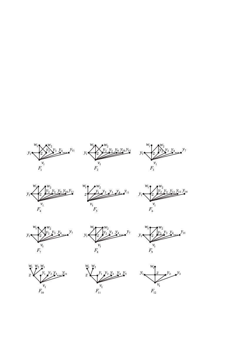
Figure 2.1: The graphs $F_{1}$, $F_{2}$, $\ldots$, $F_{12}$.

For graphs $G$ and $F$, we write $F\subset G$ if $F$ is a subgraph of $G$, and we call $F$ is forbidden to $G$ if $G$ cannot contain $F$ as its subgraph. Let $F_{1},F_{2},\ldots,F_{12}$ be the $12$ graphs as shown in Figure 2.1. By direct calculations, $\lambda_{2}(F_{i})\geq 5$, $i=1,2,\ldots,9$, and $\lambda_{2}(F_{i})>4.7$, $i=10,11,12$. Thus, if $G$ is a graph with $\lambda_{2}(G)<5$, then

each graph of $$\{ F_{i} 1\leq i\leq 9 \} G$$: is forbidden to . (2.1)

If $G$ is a graph with $\lambda_{2}(G)\leq 4.7$, then

each graph of $$\{ F_{i} 10\leq i\leq 12 \} G$$: is forbidden to . (2.2)

Moreover, let $W_{1},W_{2},\ldots,W_{7}$ be the $7$ graphs as shown in Figure 2.2. We show an upper bound and a lower bound of the first largest Laplacian eigenvalue of graphs $W_{1}$ and $W_{2}$, that is:

Lemma 2.9.

Let $W_{1}$ and $W_{2}$ be the graphs with $n\geq 5$ vertices in Fig 2.2, where $1\leq s\leq n-4$. Then $n-2<\lambda_{1}(W_{1})=\lambda_{1}(W_{2})<n-1$.

Proof. Let $v_{1},w_{1},w_{2}$ be the three vertices labeled in $W_{2}$ in Fig 2.2, where $d_{W_{2}}(v_{1})=n-3$, $d_{W_{2}}(w_{1})=s$ and $d_{W_{2}}(w_{2})=n-3-s$. The remaining vertices all have degree $2$. By Lemmas 2.2 and 2.5, $\lambda_{1}(W_{1})=\lambda_{1}(W_{2})>n-2$. Let $E_{1}$ and $E_{2}$ be the sets of edges incident with $w_{1}$ and $w_{2}$ in graph $W_{2}$, respectively. For the edges in $E(W_{2})\setminus(E_{1}\cup E_{2})$ (all incident with $v_{1}$), we let $E_{3}$ and $E_{4}$ be the sets of edges adjacent to the edges in $E_{1}$ and $E_{2}$, respectively. Then $E(W_{2})=E_{1}\cup E_{2}\cup E_{3}\cup E_{4}$.

If $uv\in E_{1}$, then

$$\Psi(uv)=\frac{s^{2}+2s+4+(s+n-3)}{s+2}=\frac{s^{2}+3s+n+1}{s+2}<n-1.$$

If $uv\in E_{2}$, then

$$\Psi(uv)=\frac{(n-3-s)^{2}+2(n-3-s)+4+(n-3+n-3-s)}{n-3-s+2}=\frac{(n-1-s)^{2}+s}{n-1-s}<n-1.$$

If $uv\in E_{3}$, then

$$\Psi(uv)=\frac{(n-3)^{2}+2(n-3)+4+(s+n-3)}{n-3+2}=\frac{(n-3)^{2}+3(n-3)+4+s}{n-1}<n-1.$$

If $uv\in E_{4}$, then

$$\Psi(uv)=\frac{(n-3)^{2}+2(n-3)+4+(n-3-s+n-3)}{n-3+2}=\frac{(n-3)^{2}+4(n-3)+4-s}{n-1}<n-1.$$

Therefore, by Lemmas 2.2 and 2.5, $\lambda_{1}(W_{1})=\lambda_{1}(W_{2})<n-1$. ∎

For a connected graph $G$, denote by $\tau(G)$ the number of triangles of $G$. The following lemma is useful.

Lemma 2.10.

[10] If $G$ is a graph with $n$ vertices and $m$ edges, then

$$\sum_{i=1}^{n}\lambda_{i}=\sum_{i=1}^{n}d_{i}=2m,\hskip 5.0pt\sum_{i=1}^{n}\lambda^{2}_{i}=2m+\sum_{i=1}^{n}d^{2}_{i},\,\text{and}\,\, \sum_{i=1}^{n}\lambda^{3}_{i}=3\sum_{i=1}^{n}d^{2}_{i}+\sum_{i=1}^{n}d^{3}_{i}-6\tau(G).$$

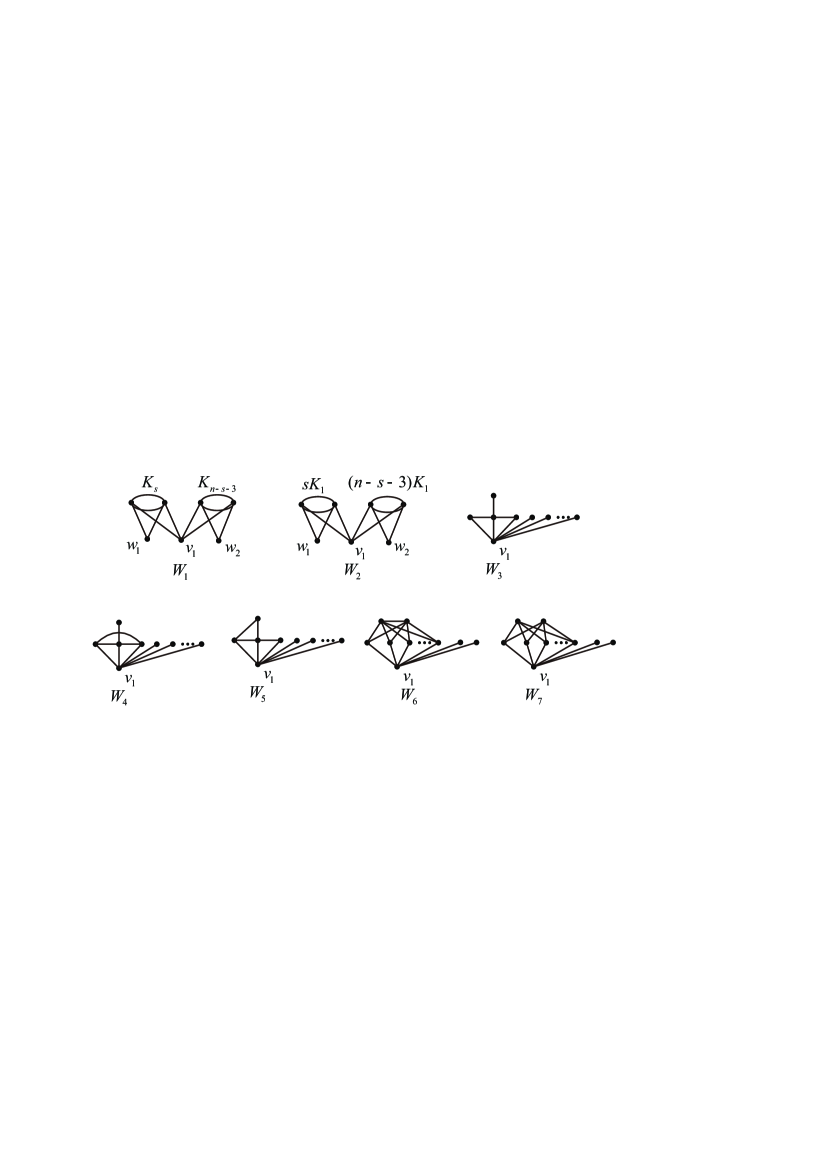
Figure 2.2: The graphs $W_{1}$, $W_{2}$, $\ldots$, $W_{7}$.

3 Proof of Theorem 1.3

Let $\operatorname{diag}\{b_{1},b_{2},...,b_{n}\}$ be a diagonal matrix with the given vectors lying on the main diagonal. And we denote by $\theta_{i}(M)$ the $i$-th largest eigenvalue of the square matrix $M$ with order $n$, where $1\leq i\leq n$.

Lemma 3.1.

[13] Let $G$ be a graph with $\left\{w_{1},w_{2},\dots,w_{s}\right\}$=W $\subseteq V(G)$. If $H\cong G[W]$, then for any $i\in\left\{1,2,\dots,s\right\}$ and $0\leq p_{i}\leq d_{G}(w_{i})$, we have $\lambda_{i}(G)\geq\theta_{i}(diag\left\{p_{1},p_{2},\dots\,p_{s}\right\}-A(H))$.

Lemma 3.2.

[18] Let $G$ be a connected graph with $n$ vertices and $d_{2}(G)\leq 4$. If either $d_{n}(G)=1<11\leq d_{1}(G)$ or $2\leq d_{n}(G)<8\leq d_{1}(G)$, then $\lambda_{1}(G)\leq\kappa_{1}(G)\leq d_{1}(G)+3$.

Next, we will use vertex-weighted graphs illustrated in Figure 3.1. They are ‘vertex-weighted’ in the sense that some of their vertices are accompanied with weights. Precisely, vertices $z_{1}$, $z_{2}$ and $z_{3}$ have weight 4, vertex $u_{1}$ has weight $3$, and weight $d(v_{1})$ of $v_{1}$ is as in the figure. These graphs can be seen as subgraphs of larger graphs, say $R^{\prime}_{1},R^{\prime}_{2},\ldots,R^{\prime}_{10}$, in which degrees of the previously mentioned vertices are equal to given weights. We don’t need to know the exact distribution of other edges, but we care about the vertex degrees, and that is why they are interpreted as weights. More succinctly, we use the same notation for vertex weights and vertex degrees. Therefore, for $1\leq i\leq 10$, the matrix representation of $R_{i}$, say $L^{*}(R_{i})$, is the principal submatrix of the Laplacian matrix $L(R^{\prime}_{i})$.

Remark 3.1.

In what follows, we consider graphs $G$ that contain some of graphs $R^{\prime}_{i},1\leq i\leq 10$, as subgraphs, and in each situation we estimate $\lambda_{2}(G)$ as demonstrated in this remark. Take, for example, that a graph $G$ contains $R^{\prime}_{8}$ as a subgraph $($Notice that $u_{1}$ has weight $3$ in $R_{8}$ in Fig 3.1, which means that there exists some vertex, say $z$, such that $z\in V(R^{\prime}_{8})\setminus V(R_{8})$ and $zu_{1}\in E(R^{\prime}_{8})$$)$. Then $L^{*}(R_{8})$ is a principal submatrix of $L(R^{\prime}_{8})$. By Lemmas 2.8 and 3.1, we have $\lambda_{2}(G)\geq\theta_{2}(L^{*}(R_{8}))>5$ when $d_{R^{\prime}_{8}}(v_{1})\geq 5$, where

$L^{*}(R_{8})=\begin{pmatrix}&d_{R^{\prime}_{8}}(v_{1})&-1&-1&-1&0\\ &-1&4&-1&-1&-1\\ &-1&-1&3&0&0\\ &-1&-1&0&2&0\\ &0&-1&0&0&1\end{pmatrix}$.

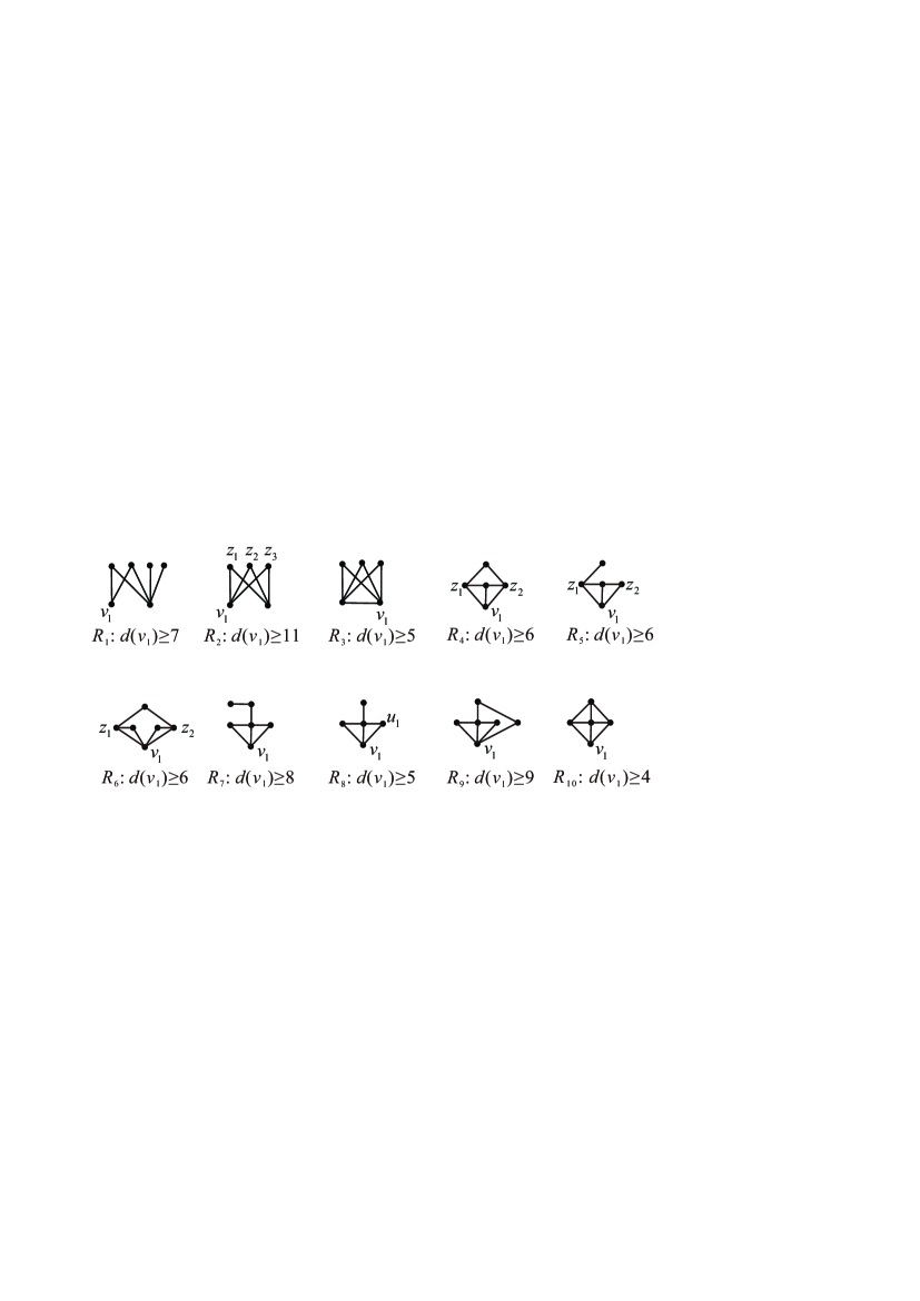
Figure 3.1: The graphs $R_{1}$, $R_{2}$, $\ldots$, $R_{10}$.

Lemma 3.3.

Let $G$ be a connected graph with $n\geq 15$ vertices such that $\lambda_{2}(G)<5$ and $d_{1}(G)\geq n-4$. Then, $d_{2}(G)\leq 4$ and any two $4$-vertices (if exist) are not adjacent. Moreover, if $w\notin\{v_{1}\}\cup N_{G}(v_{1})$, then $d_{G}(w)\leq 3$ and $w$ is adjacent to at most two $4$-vertices.

Proof. By Lemma 2.6, we have $d_{2}(G)\leq 4$ since $\lambda_{2}(G)<5$. Let $w$ be a vertex with $w\notin\{v_{1}\}\cup N_{G}(v_{1})$ (if exists). If $d_{G}(w)=4$, then by Lemmas 2.8 and 3.1 we have $\lambda_{2}(G)\geq\theta_{2}({L}^{*}(R_{1}))\geq 5$, a contradiction. Thus $d_{G}(w)\leq 3$. This implies that every 4-vertex is adjacent to $v_{1}$. Assume that there exists two 4-vertices being adjacent, then the two 4-vertices and $v_{1}$ induces a triangle. One can easily check that $\lambda_{2}(G)\geq 5$ when $d_{G}(v_{1})\geq 4$ by Lemma 3.1, a contradiction. So we can conclude that any two $4$-vertices (if exist) are not adjacent.

Next, we show that $w$ is adjacent to at most two 4-vertices. Otherwise, suppose that $d_{G}(w)=3$ and $w$ is adjacent to three 4-vertices. Then, the three 4-vertices induces an independent set of $G$, and then by Lemmas 2.8 and 3.1 we have $\lambda_{2}(G)\geq\theta_{2}(L^{*}(R_{2}))\geq 5$, a contradiction. ∎

Lemma 3.4.

Let $G$ be a connected graph with $n\geq 15$ vertices, $d_{2}(G)=4$ and $\lambda_{2}(G)<5<n-1<\lambda_{1}(G)$. Then $n-3\leq d_{1}(G)\leq n-2$ and $n_{4}(G)=1$. Moreover, $zv_{1}\in E(G)$ and $1\leq|N_{G}(z)\cap N_{G}(v_{1})|\leq 2$, where $z$ is the unique $4$-vertex of $G$.

Proof. Since $d_{2}(G)=4$ and $n-1<\lambda_{1}(G)\leq d_{1}(G)+4$ (by Lemma 2.5), we have $d_{1}(G)\geq n-4\geq 11$. In view of Lemma 3.2, it follows that $d_{1}(G)\geq n-3$. Let $z$ be a 4-vertex of $G$. By Lemma 3.3, we have $zv_{1}\in E(G)$. Note that $d_{G}(v_{1})\geq n-3$, so $\left|N_{G}(z)\cap N_{G}(v_{1})\right|\geq 1$. If $\left|N_{G}(z)\cap N_{G}(v_{1})\right|=3$, then by Lemmas 2.8 and 3.1, we have $\lambda_{2}(G)\geq\theta_{2}(L^{*}(R_{3}))\geq 5$, a contradiction. Thus, $1\leq|N_{G}(z)\cap N_{G}(v_{1})|\leq 2$ and $n-3\leq d_{1}(G)\leq n-2$.

Next, we show that $n_{4}(G)=1$. By contradiction, assume that $n_{4}(G)\geq 2$ and $z_{1},z_{2}$ are two 4-vertices of $G$. By Lemma 3.3, $z_{1}z_{2}\not\in E(G)$ and $\{z_{1},z_{2}\}\subset N_{G}(v_{1})$. Since $1\leq|N_{G}(z_{1})\cap N_{G}(v_{1})|\leq 2$, we can suppose $w_{1}\in N_{G}(z_{1})\setminus(N_{G}(v_{1})\cup\{v_{1}\})$. If there exists $u\in N_{G}(v_{1})$ such that $u\in N_{G}(z_{1})\cap N_{G}(z_{2})$, then either $\lambda_{2}(G)\geq\theta_{2}(L^{*}(R_{4}))\geq 5$ ($w_{1}z_{2}\in E(G)$) or $\lambda_{2}(G)\geq\theta_{2}(L^{*}(R_{5}))\geq 5$ ($w_{1}z_{2}\notin E(G)$), a contradiction. Thus, $N_{G}(z_{1})\cap N_{G}(z_{2})\cap N_{G}(v_{1})=\mbox{{\rm\O}}$.

Now, note that $1\leq|N_{G}(z_{2})\cap N_{G}(v_{1})|\leq 2$, if $w_{1}z_{2}\in E(G)$, then $\lambda_{2}(G)\geq\theta_{2}(L^{*}(R_{6}))\geq 5$, a contradiction. So we can suppose $w_{2}\in N_{G}(z_{2})\setminus(N_{G}(v_{1})\cup\{v_{1}\})$ and $w_{2}\neq w_{1}$. And hence $d_{1}(G)=n-3$. If $n_{4}(G)\geq 3$, we assume that $z_{3}$ is an another $4$-vertex. Then from above statements, we have either $w_{1}z_{3}\in E(G)$ or $w_{2}z_{3}\in E(G)$. And so $\lambda_{2}(G)\geq\theta_{2}(L^{*}(R_{6}))\geq 5$, a contradiction. Thus $n_{4}(G)=2$. Now we would like to show that $N_{G}(w_{i})\setminus\{z_{i}\}\subset N_{G}(z_{i})$, $i\in\{1,2\}$. Otherwise, $\lambda_{2}(G)\geq\theta_{2}(L^{*}(R_{7}))\geq 5$, a contradiction. Note that $N_{G}(z_{1})\cap N_{G}(z_{2})=\{v_{1}\}$. It is easy to see that $w_{1}$ and $w_{2}$ are in different components of $G-v_{1}$ (Otherwise $\lambda_{2}(G)\geq\theta_{2}(L^{*}(R_{8}))\geq 5$). So $G$ is a subgraph of $W_{1}$ in Fig 2.2. By Lemmas 2.8 and 2.9, $\lambda_{1}(G)\leq\lambda_{1}(W_{1})=\lambda_{1}(W_{2})<n-1$, a contradiction. This confirms $n_{4}(G)=1$. ∎

Proof of Theorem 1.3. Since $G$ is connected, $\lambda_{n-1}(G)>0$. Then $\lambda_{n-1}(H)=\lambda_{n-1}(G)>0$, so $H$ is also connected. For short, next we write $n_{i}(G)$, $d_{j}(G)$, $n_{i}(H)$ and $d_{j}(H)$ as $n_{i}$, $d_{j}$, $n_{i}^{*}$ and $d_{j}^{*}$, respectively, where $i\in\{1,2,3,4\}$ and $j\in\{1,2,\ldots,n\}$. Without loss of generality, we suppose $d_{1}\leq d^{*}_{1}$. By Lemmas 2.6 and 2.5, we have $d_{2}\leq 4$, $d_{2}^{*}\leq 4$, $d_{1}\geq n-4$ and $d_{1}^{*}\geq n-4$. Since $n-4>11$, it follows from Lemma 3.2 that $d_{1}\geq n-3$ and $d_{1}^{*}\geq n-3$. Since $K_{1,n-1}$ is determined by its Laplacian spectrum (see [11]), taking Lemma 2.7 into consideration, we may suppose that $d_{2}\geq 3$ and $d_{2}^{*}\geq 3$.

From Lemma 2.10, we have

$$\left\{\begin{array}[]{ll}&2n_{3}^{*}+6n_{4}^{*}+d_{1}^{*}(d_{1}^{*}-3)=2n_{3}+6n_{4}+d_{1}(d_{1}-3),\\ &n_{2}^{*}-3n_{4}^{*}-d_{1}^{*}(d_{1}^{*}-4)=n_{2}-3n_{4}-d_{1}(d_{1}-4),\\ &2n_{1}^{*}+2n_{4}^{*}+d_{1}^{*}(d_{1}^{*}-5)=2n_{1}+2n_{4}+d_{1}(d_{1}-5).\end{array}\right.$$ (3.1)

We claim that $d_{1}=d^{*}_{1}$. Conversely we assume that $d_{1}<d^{*}_{1}$. Then, $n-3\leq d_{1}<d^{*}_{1}\leq n-1$. Note that $d_{2}^{*}\geq 3$, so $n-2\geq n^{*}_{2}=\big{(}n_{2}+3n^{*}_{4}+d^{*}_{1}(d^{*}_{1}-4)-d_{1}(d_{1}-4)-3n_{4}\big{)}$ by (3.1). By Lemma 3.4, we know $n_{4}\leq 1$. And note that there are three possibilities for $d_{1}$ and $d^{*}_{1}$: If $d_{1}^{*}=n-1$ and $d_{1}=n-2$, then $n-2\geq d^{*}_{1}(d^{*}_{1}-4)-d_{1}(d_{1}-4)-3=2n-10$. And hence $n\leq 8$, contrary with $n\geq 18$; If $d_{1}^{*}=n-1$ and $d_{1}=n-3$, then $n-2\geq d^{*}_{1}(d^{*}_{1}-4)-d_{1}(d_{1}-4)-3=4n-19$. And hence $n\leq 5$, contrary with $n\geq 18$; If $d_{1}^{*}=n-2$ and $d_{1}=n-3$, then $n-2\geq d^{*}_{1}(d^{*}_{1}-4)-d_{1}(d_{1}-4)-3=2n-12$. And hence $n\leq 10$, contrary with $n\geq 18$. This confirms $d_{1}=d^{*}_{1}$.

Now combining $d_{1}=d^{*}_{1}$ with (3.1), we have

$$\left\{\begin{array}[]{ll}&n_{3}^{*}+3n_{4}^{*}=n_{3}+3n_{4},\\ &n_{2}^{*}-3n_{4}^{*}=n_{2}-3n_{4},\\ &n_{1}^{*}+n_{4}^{*}=n_{1}+n_{4}.\end{array}\right.$$ (3.2)

From (3.2), if $n_{4}=n^{*}_{4}$, then $n_{i}=n_{i}^{*}$, $i=1,2,3$. The result already holds. Next, without loss of generality, we conversely assume that $n_{4}>n^{*}_{4}$. By Lemma 3.4, we know $n_{4}\leq 1$. So $0=n^{*}_{4}<n_{4}=1$. Combining this with (3.2), we have

$$\left\{\begin{array}[]{ll}&n_{3}^{*}=n_{3}+3,\\ &n_{2}^{*}=n_{2}-3,\\ &n_{1}^{*}=n_{1}+1.\end{array}\right.$$ (3.3)

By Lemma 3.4, we obtain that $n-3\leq d^{*}_{1}=d_{1}\leq n-2$ as $n_{4}=1$.

Case 1. $d_{1}=d^{*}_{1}=n-2$. Suppose that $z$ is the unique 4-vertex of $G$, $d_{G}(v_{1})=n-2$ and $w_{1}=V(G)\setminus(N_{G}(v_{1})\cup\{v_{1}\})$. By Lemma 3.3, we have $zv_{1}\in E(G)$. Obviously, $zw_{1}\in E(G)$ (Otherwise $\lambda_{2}(G)\geq\theta_{2}(L^{*}(R_{3}))\geq 5$). Suppose that $N_{G}(z)=\{v_{1},w_{1},w_{2},w_{3}\}$. By Lemma 3.3, $1\leq d_{G}(w_{1})\leq 3$ and $2\leq d_{G}(w_{i})\leq 3$, $i=2,3$.

Subcase 1.1. $d_{G}(w_{1})=1$. $(i)$: If $d_{G}(w_{2})=d_{G}(w_{3})=2$, then by Lemma 2.1 or Lemma 2.2, $\lambda_{1}(G)=\lambda_{1}(W_{3})$, a contradiction. $(ii)$: If $d_{G}(w_{2})=3>d_{G}(w_{3})=2$ or $d_{G}(w_{2})=2<d_{G}(w_{3})=3$, then by Lemma 3.1, $\lambda_{2}(G)\geq\theta_{2}(L^{*}(R_{8}))\geq 5$, a contradiction. $(iii)$: $d_{G}(w_{2})=d_{G}(w_{3})=3$. If $w_{2}w_{3}\notin E(G)$, then by Lemmas 2.8 and 3.1, $\lambda_{2}(G)\geq\theta_{2}(L^{*}(R_{8}))\geq 5$, a contradiction. Otherwise, $w_{2}w_{3}\in E(G)$. But now by Lemmas 2.1 and 2.2, $\lambda_{1}(G)=\lambda_{1}(W_{4})=\lambda_{1}(W_{3})$, a contradiction.

Subcase 1.2. $d_{G}(w_{1})=2$. $(i)$: If $w_{1}w_{2}\in E(G)$ or $w_{1}w_{3}\in E(G)$, by symmetry we just consider $w_{1}w_{2}\in E(G)$. $(a)$: If $d_{G}(w_{3})=3$, then $\lambda_{2}(G)\geq\lambda_{2}(G-w_{1}w_{2})\geq\theta_{2}(L^{*}(R_{8}))\geq 5$, a contradiction. $(b)$: If $d_{G}(w_{3})=2$, then by Lemma 2.1, $\lambda_{1}(G)=\lambda_{1}(W_{5})$, a contradiction. $(ii)$: If $w_{1}w_{2}\notin E(G)$ and $w_{1}w_{3}\notin E(G)$, then $\lambda_{2}(G)\geq\theta_{2}(L^{*}(R_{9}))\geq 5$, a contradiction.

Subcase 1.3. $d_{G}(w_{1})=3$. $(i)$: If $w_{1}w_{2}\notin E(G)$ and $w_{1}w_{3}\notin E(G)$, then $\lambda_{2}(G)\geq\theta_{2}(L^{*}(R_{9}))\geq 5$, a contradiction. $(ii)$: If exactly one vertex of $\{w_{2},w_{3}\}$ is adjacent to $w_{1}$, then by Lemmas 2.8 and 3.1, we have $\lambda_{2}(G)\geq\theta_{2}(L^{*}(R_{9}))\geq 5$, a contradiction. $(iii)$: If $w_{1}w_{2}\in E(G)$ and $w_{1}w_{3}\in E(G)$, then $\lambda_{2}(G)\geq\theta_{2}(L^{*}(R_{10}))\geq 5$, a contradiction.

Case 2. $d_{1}=d^{*}_{1}=n-3$. Let $V(G)\setminus N_{G}(v_{1})=\{w_{1},w_{2},v_{1}\}$. If $w_{1}$ and $w_{2}$ are in different components of $G-v_{1}$, then $G$ is a subgraph of $W_{1}$. By Lemmas 2.8 and 2.9, $\lambda_{1}(G)\leq\lambda_{1}(W_{1})=\lambda_{1}(W_{2})<n-1$, a contradiction. Thus, $w_{1}$ and $w_{2}$ are in the same component, say $G_{1}$, of $G-v_{1}$. Let $G_{2}=(G-v_{1})-V(G_{1})$. By Lemma 2.1 , we have $\lambda_{1}(G)=\lambda_{1}(\widetilde{G})$, where $\widetilde{G}$ is obtained from $G$ by deleting all edges of $E(G_{2})$. Note that $d_{2}=4$ and $n_{4}=1$. If $|V(G_{2})|\geq 2$, by Lemmas 2.2 and 2.8, then $\lambda_{1}(G)=\lambda_{1}(\widetilde{G})\leq\lambda_{1}(W_{6})=\lambda_{1}(W_{7})<n-1$, a contradiction. Thus, $|V(G_{2})|\leq 1$ and $n-2\leq|V(G_{1})|\leq n-1$.

Let $z$ be the unique 4-vertex of $G$. By Lemma 3.3, we have $zv_{1}\in E(G)$. Moreover, $1\leq|N_{G}(z)\cap N_{G}(v_{1})|\leq 2$ by Lemma 3.4. So at least one of $\{w_{1},w_{2}\}$ is adjacent to $z$, without loss of generality, we suppose $w_{1}z\in E(G)$. Next we would like to show that $|N_{G}(z)\cap N_{G}(v_{1})|=1$. By contradiction, we assume that $|N_{G}(z)\cap N_{G}(v_{1})|=2$ and $N_{G}(z)\cap N_{G}(v_{1})=\{y_{1},y_{2}\}$. Now, obviously, $N_{G}(w_{1})\subset\{z,y_{1},y_{2}\}$, otherwise $\lambda_{2}(G)\geq\theta_{2}(L^{*}(R_{7}))\geq 5$, a contradiction. And $N_{G}(y_{i})\subset\{z,v_{1},w_{1}\}$, $i=1,2$, otherwise $\lambda_{2}(G)\geq\theta_{2}(L^{*}(R_{8}))\geq 5$, a contradiction. However, it means that $w_{1}$ and $w_{2}$ are in different components of $G-v_{1}$, a contradiction. So we can conclude that $|N_{G}(z)\cap N_{G}(v_{1})|=1$, $zw_{1}\in E(G)$ and $zw_{2}\in E(G)$. For convenience, from now on we suppose $N_{G}(z)\cap N_{G}(v_{1})=\{y_{1}\}$ and $N_{G}(v_{1})=\{z,y_{1},y_{2},\ldots,y_{n-4}\}$.

Subcase 2.1. $w_{1}w_{2}\notin E(G)$.

Subcase 2.1.1. $w_{1}y_{1}\in E(G)$ or $w_{2}y_{1}\in E(G)$. Note that $n_{4}=1$ and $d_{2}=4$, so in this case, exactly one vertex of $\{w_{1},w_{2}\}$ is adjacent to $y_{1}$. By symmetry, we may suppose that $w_{1}y_{1}\in E(G)$. Then $2\leq d_{G}(w_{1})\leq 3$ and $1\leq d_{G}(w_{2})\leq 3$.

$(i)$: $d_{G}(w_{1})=3$. And we may suppose $w_{1}y_{2}\in E(G)$. $(a)$: If $d_{G}(w_{2})=2$ and $w_{2}y_{2}\in E(G)$, then $\lambda_{1}(G)\leq\lambda_{1}(W_{7})<n-1$ since $d_{2}=4$ and $n_{4}=1$, a contradiction. $(b)$: If $d_{G}(w_{2})=2$ and $w_{2}y_{2}\notin E(G)$, then $\lambda_{2}(G)\geq\lambda_{2}(F_{1})\geq 5$, a contradiction. $(c)$: If $d_{G}(w_{2})=3$, then $\lambda_{2}(G)\geq\lambda_{2}(F_{1})\geq 5$, a contradiction. $(d)$: Otherwise $d_{G}(w_{2})=1$. Note that $n-2\leq|V(G_{1})|\leq n-1$, $n_{4}=1$, $d_{2}=4$ and $n\geq 18$. So it is easy to see that $F_{2}\subset G$. And hence $\lambda_{2}(G)\geq\lambda_{2}(F_{2})>5$, a contradiction.

$(ii)$: $d_{G}(w_{1})=2$. $(a)$: If $d_{G}(w_{2})=3$, then $\lambda_{2}(G)\geq\lambda_{2}(F_{3})>5$, a contradiction. $(b)$: If $d_{G}(w_{2})=1$, then $\lambda_{1}(G)\leq\lambda_{1}(W_{7})<n-1$ since $d_{2}=4$ and $n_{4}=1$, a contradiction. $(c)$: Otherwise $d_{G}(w_{2})=2$. Note that $n-2\leq|V(G_{1})|\leq n-1$, $n_{4}=1$, $d_{2}=4$ and $n\geq 18$. So it is easy to see that $F_{4}\subset G$. And hence $\lambda_{2}(G)\geq\lambda_{2}(F_{4})>5$, a contradiction.

Subcase 2.1.2. $w_{1}y_{1}\notin E(G)$ and $w_{2}y_{1}\notin E(G)$. In this case, we claim that $d_{G}(y_{1})=2$. Otherwise $d_{G}(y_{1})=3$. Then $F_{5}\subset G$ and $\lambda_{2}(G)\geq\lambda_{2}(F_{5})>5$, a contradiction. So $N_{G}(y_{1})=\{z,v_{1}\}$.

$(i)$: $d_{G}(w_{1})=d_{G}(w_{2})=1$. Then $\lambda_{1}(G)\leq\lambda_{1}(W_{7})<n-1$, a contradiction.

$(ii)$: $\{d_{G}(w_{1}),d_{G}(w_{2})\}=\{1,2\}$. By symmetry, we may suppose that $d_{G}(w_{1})=1$ and $d_{G}(w_{2})=2$. Note that $n-2\leq|V(G_{1})|\leq n-1$, $n_{4}=1$, $d_{2}=4$ and $n\geq 18$. So it is easy to see that $F_{6}\subset G$. And hence $\lambda_{2}(G)\geq\lambda_{2}(F_{6})>5$, a contradiction.

$(iii)$: $\{d_{G}(w_{1}),d_{G}(w_{2})\}=\{1,3\}$. By symmetry, we may suppose that $d_{G}(w_{1})=1$ and $d_{G}(w_{2})=3$. Then it is easy to see that $F_{3}\subset G$. And hence $\lambda_{2}(G)\geq\lambda_{2}(F_{3})>5$, a contradiction.

$(iv)$: $d_{G}(w_{1})\geq 2$ and $d_{G}(w_{2})\geq 2$. If $|N_{G}(w_{1})\cap N_{G}(w_{2})|\geq 2$, then $F_{7}\subset G$ and $\lambda_{2}(G)\geq\lambda_{2}(F_{7})>5$, a contradiction. Otherwise, $|N_{G}(w_{1})\cap N_{G}(w_{2})|=1$. Then $F_{1}\subset G$ and $\lambda_{2}(G)\geq\lambda_{2}(F_{1})\geq 5$, a contradiction.

Subcase 2.2. $w_{1}w_{2}\in E(G)$. In this case, $2\leq d_{G}(w_{i})\leq 3$, $i=1,2$. As before, we will consider some subcases as following.

Subcase 2.2.1. $w_{1}y_{1}\in E(G)$ or $w_{2}y_{1}\in E(G)$. Note that $n_{4}=1$ and $d_{2}=4$, so in this case, exactly one vertex of $\{w_{1},w_{2}\}$ is adjacent to $y_{1}$. By symmetry, we may suppose that $w_{1}y_{1}\in E(G)$. Then $d_{G}(w_{1})=3$ and $2\leq d_{G}(w_{2})\leq 3$. If $d_{G}(w_{2})=2$, then by Lemmas 2.2 and 2.8, $\lambda_{1}(G)=\lambda_{1}(\widetilde{G})\leq\lambda_{1}(\widetilde{G}+y_{1}w_{2})\leq\lambda_{1}(W_{6})=\lambda_{1}(W_{7})<n-1$, a contradiction. Otherwise, $d_{G}(w_{2})=3$. Then $F_{8}\subset G$ and $\lambda_{2}(G)\geq\lambda_{2}(F_{8})>5$, a contradiction.

Subcase 2.2.2. $w_{1}y_{1}\notin E(G)$ and $w_{2}y_{1}\notin E(G)$.

$(i)$: $d_{G}(w_{1})=d_{G}(w_{2})=2$. If $d_{G}(y_{1})=2$, then by Lemmas 2.2 and 2.8, $\lambda_{1}(G)=\lambda_{1}(\widetilde{G})\leq\lambda_{1}(W_{6})=\lambda_{1}(W_{7})<n-1$, a contradiction. Otherwise, $d_{G}(y_{1})=3$. Then $F_{5}\subset G$ and $\lambda_{2}(G)\geq\lambda_{2}(F_{5})>5$, a contradiction.

$(ii)$: $\{d_{G}(w_{1}),d_{G}(w_{2})\}=\{2,3\}$. By symmetry, we may suppose that $d_{G}(w_{1})=2$, $d_{G}(w_{2})=3$ and $w_{2}y_{2}\in E(G)$ ($y_{2}\notin\{y_{1},w_{1},z\}$). Note that $F_{5}\not\subset G$, so $d_{G}(y_{1})\not=3$, i.e. $d_{G}(y_{1})=2$. Then it is easy to see that $F_{9}\subset G$ since $n-2\leq|V(G_{1})|\leq n-1$, $n_{4}=1$, $d_{2}=4$ and $n\geq 18$. And hence $\lambda_{2}(G)\geq\lambda_{2}(F_{9})\geq 5$, a contradiction.

$(iii)$: $d_{G}(w_{1})=d_{G}(w_{2})=3$. If $|N_{G}(w_{1})\cap N_{G}(w_{2})|\geq 2$, then $F_{7}\subset G$ and $\lambda_{2}(G)\geq\lambda_{2}(F_{7})>5$, a contradiction. Otherwise, $|N_{G}(w_{1})\cap N_{G}(w_{2})|=1$. Then $F_{1}\subset G$ and $\lambda_{2}(G)\geq\lambda_{2}(F_{1})\geq 5$, a contradiction.

In summary, we can conclude that if graphs G and H satisfy the conditions of Theorem 1.3, then G and H must be co-degree. ∎

In view of the proof of Theorem 1.3, we can easily obtain the following corollary:

Corollary 3.1.

Let $G$ be a connected graph with $n\geq 18$ vertices and $\lambda_{2}(G)<5<n-1<\lambda_{1}(G)$. If $d_{1}(G)\neq n-2$ and $S_{L}(H)=S_{L}(G)$, then $H$ and $G$ are co-degree.

4 Proofs of Theorem 1.4 and Corollaries 1.1 and 1.2

Lemma 4.1.

Let $G$ be a connected graph with $n\geq 16$ vertices. If $\lambda_{2}(G)\leq 4.7<n-2<\lambda_{1}(G)$, then $d_{2}(G)\leq 3$ and $d_{1}(G)\geq n-4$.

Proof. Since $\lambda_{2}(G)\leq 4.7$, by Lemma 2.6, $d_{2}(G)\leq 4$. Then $n-2<\lambda_{1}(G)\leq d_{1}(G)+4$ by Lemma 2.5, so $d_{1}(G)\geq n-5\geq 11$. Now, by Lemma 3.2, we have $n-2<\lambda_{1}(G)\leq d_{1}(G)+3$, so $d_{1}(G)\geq n-4$.

Next we will show that $d_{2}(G)\leq 3$. By contradiction, we assume that $d_{2}(G)=4$ and $z$ is a 4-vertex. By Lemma 3.3, $zv_{1}\in E(G)$. If $|N_{G}(z)\cap N_{G}(v_{1})|=0$, then $F_{10}\subset G$, so $\lambda_{2}(G)\geq\lambda_{2}(F_{10})>4.7$, a contradiction; If $|N_{G}(z)\cap N_{G}(v_{1})|=1$, then $F_{11}\subset G$, so $\lambda_{2}(G)\geq\lambda_{2}(F_{11})>4.7$, a contradiction; If $|N_{G}(z)\cap N_{G}(v_{1})|=2$, then $F_{12}\subset G$, so $\lambda_{2}(G)\geq\lambda_{2}(F_{12})>4.7$, a contradiction; If $|N_{G}(z)\cap N_{G}(v_{1})|=3$, then by Lemmas 2.8 and 3.1, we have $\lambda_{2}(G)\geq\theta_{2}(L^{*}(R_{3}))\geq 5>4.7$, a contradiction. Therefore, $n_{4}(G)=0$ and $d_{2}(G)\leq 3$. ∎

Proof of Theorem 1.4. By Lemma 4.1, $d_{2}(G)\leq 3$, $d_{2}(H)\leq 3$, $d_{1}(G)\geq n-4$ and $d_{1}(H)\geq n-4$. In the following, we simplify $n_{i}(G)$, $n_{i}(H)$, $d_{1}(G)$ and $d_{1}(H)$ as $n_{i}$, $n_{i}^{*}$, $d_{1}$ and $d_{1}^{*}$, respectively, where $i\in\{1,2,3\}$. Since $K_{1,n-1}$ is determined by its Laplacian spectrum (see [11]), taking Lemma 2.7 into consideration, we may suppose that $d_{2}=d_{2}^{*}=3$. And without loss of generality, we suppose $d_{1}\leq d_{1}^{*}$. By Lemma 2.10, we have

$$\left\{\begin{array}[]{lll}n^{*}_{1}+n^{*}_{2}+n^{*}_{3}=n_{1}+n_{2}+n_{3},\\ n^{*}_{1}+2n^{*}_{2}+3n^{*}_{3}+d^{*}_{1}=n_{1}+2n_{2}+3n_{3}+d_{1},\\ n^{*}_{1}+4n^{*}_{2}+9n^{*}_{3}+(d^{*}_{1})^{2}=n_{1}+4n_{2}+9n_{3}+(d_{1})^{2}.\end{array}\right.$$ (4.4)

From (4.4), it is easy to get that

$$n^{*}_{2}=n_{2}+d^{*}_{1}(d^{*}_{1}-4)-d_{1}(d_{1}-4).$$ (4.5)

We claim that $d_{1}=d^{*}_{1}$. Conversely we assume that $d_{1}<d^{*}_{1}$. Then, $n-4\leq d_{1}<d^{*}_{1}\leq n-1$. Since $d_{2}^{*}=3$, we get $n-2\geq n^{*}_{2}\geq d^{*}_{1}(d^{*}_{1}-4)-d_{1}(d_{1}-4)$ by (4.5). And note that there are six possibilities for $d_{1}$ and $d^{*}_{1}$: If $d_{1}^{*}=n-1$ and $d_{1}=n-2$, then $n-2\geq d^{*}_{1}(d^{*}_{1}-4)-d_{1}(d_{1}-4)=2n-7$. And hence $n\leq 5$, contrary with $n\geq 16$; If $d_{1}^{*}=n-1$ and $d_{1}=n-3$, then $n-2\geq d^{*}_{1}(d^{*}_{1}-4)-d_{1}(d_{1}-4)=4n-16$. And hence $n\leq 4$, contrary with $n\geq 16$; If $d_{1}^{*}=n-1$ and $d_{1}=n-4$, then $n-2\geq d^{*}_{1}(d^{*}_{1}-4)-d_{1}(d_{1}-4)=6n-27$. And hence $n\leq 5$, contrary with $n\geq 16$; If $d_{1}^{*}=n-2$ and $d_{1}=n-3$, then $n-2\geq d^{*}_{1}(d^{*}_{1}-4)-d_{1}(d_{1}-4)=2n-9$. And hence $n\leq 7$, contrary with $n\geq 16$; If $d_{1}^{*}=n-2$ and $d_{1}=n-4$, then $n-2\geq d^{*}_{1}(d^{*}_{1}-4)-d_{1}(d_{1}-4)=4n-20$. And hence $n\leq 6$, contrary with $n\geq 16$; If $d_{1}^{*}=n-3$ and $d_{1}=n-4$, then $n-2\geq d^{*}_{1}(d^{*}_{1}-4)-d_{1}(d_{1}-4)=2n-11$. And hence $n\leq 9$, contrary with $n\geq 16$. This confirms $d_{1}=d^{*}_{1}$.

Now combining $d_{1}=d^{*}_{1}$ with (4.5), we get $n_{2}^{*}=n_{2}$. Then by (4.4), it is easy to see that $n_{1}^{*}=n_{1}$ and $n_{3}^{*}=n_{3}$. Therefore, $G$ and $H$ are co-degree. ∎

Proof of Corollary 1.1. For convenience, let $G:=K_{1}\vee(P_{l_{1}}\cup P_{l_{1}}\cup\cdots\cup P_{l_{t}})=K_{1}\vee(sP_{1}\cup P_{l_{s+1}}\cup P_{l_{s+2}}\cup\cdots\cup P_{l_{t}})$ ($2\leq l_{s+1}\leq l_{s+2}\leq\cdots\leq l_{t}$), $n:=1+\sum_{i=1}^{t}l_{i}$ and $H$ be $L$-cospectral with $G$. By Corollary 2.2 and Lemma 2.4, $\lambda_{1}(G)=n\notin\{\lambda_{1}(W_{3}),\lambda_{1}(W_{5})\}$ and $\lambda_{2}(G)=3+2\cos\pi/l_{t}<5$. When $n\leq 17$, it is easy to check that $H=G$ by Lemmas 2.4, 2.5 and 2.6. So we suppose $n\geq 18$. By Theorem 1.3, $H$ and $G$ must be co-degree. Obviously, $H=K_{1}\vee(sP_{1}\cup P_{n_{s+1}}\cup P_{n_{s+2}}\cup\cdots\cup P_{n_{t}})$ or $H=K_{1}\vee(sP_{1}\cup P_{n_{s+1}}\cup P_{n_{s+2}}\cup\cdots\cup P_{n_{t}}\cup C_{q_{1}}\cup C_{q_{2}}\cdots\cup C_{q_{k}})$ ($2\leq n_{s+1}\leq n_{s+2}\leq\cdots\leq n_{t},k\geq 1$). But now combining this with Corollary 2.2, $H=G$, i.e. $G$ is $DLS$. ∎

Proof of Corollary 1.2. For convenience, let $G:=K_{1}\vee(P_{l_{1}}\cup P_{l_{1}}\cup\cdots\cup P_{l_{t}}\cup C_{s_{1}}\cup C_{s_{2}}\cup\cdots\cup C_{s_{k}})$ $(t\geq 1,k\geq 1)$ with $n\geq 18$ vertices and $H$ be $L$-cospectral with $G$. By Corollary 2.2 and Lemma 2.4, $\lambda_{1}(G)=n\notin\{\lambda_{1}(W_{3}),\lambda_{1}(W_{5})\}$. Moreover, if each $s_{i}$ $(i=1,2,\ldots,k)$ is odd, then $\lambda_{2}(G)<5$ by Corollary 2.2. Then by Theorem 1.3, $H$ and $G$ must be co-degree. Similar with the proof of Corollary 1.1, it is easy to see that $H=G$ by Corollary 2.2, i.e. $G$ is $DLS$. ∎

References

[1] E.R. van Dam, W.H. Haemers, Which graphs are determined by their
spectrum? Linear Algebra Appl., 373 (2003), 241–272.
[2]E.R. van Dam, W.H. Haemers, Developments on spectral characterizations of graphs, Discrete Math., 309 (2009), 576–586.
[3] K.C. Das, The
Laplacian sprectrum of a graph, Comput. Appl. Math., 48
(2004), 715–724.
[4] H.H. Günthard, H. Primas, Zusammenhang von Graphtheorie und Mo-Theotie von Molekeln mit Systemen konjugierter Bindungen, Helv. Chim. Acta, 39 (1956), 1645–1653.
[5] J.-M. Guo, The Laplcian spectral radius of a graph under perturbation, Comput. Appl. Math., 54 (2007), 709–720.
[6] J.V.D. Heuvel, Hamilton cycles and eigenvalues of
graphs, Linear Algebra Appl., 226-228 (1995), 723–730.
[7]A.K. Kelmans, The number of trees in a graph I, II, Automat. Remote Control 26 (1965) 2118–2129 and 27 (1966) 233–241 (Translated from
Avtomat. i Telemekh. 26 (1965) 2194–2204 and 27 (1966) 56–65 [in Russian]).
[8]J.S. Li, Y.L. Pan, A note on the second largest eigenvalue of the Laplacian matrix of a graph, Linear Multilinear Algebra, 48 (2000), 117–121.
[9]B. Liu, Z. Chen, M. Liu, On graphs with the largest Laplacian index, Czechoslovak Math. J., 58 (2008), 949–960.
[10]M. Liu, Some graphs determined by their (signless) Laplacian spectra, Czechoslovak Math. J., 62 (2012), 1117–1134.
[11] M. Liu, X. Tan, B. Liu, The (signless) Laplacian spectral radius of unicyclic and bicyclic graphs with vertices and pendant vertices, Czechoslovak Math. J., 60 (2010), 849–867.
[12] M. Liu, Y. Yuan, L. You, Z. Chen, Which cospectral graphs have same degree sequences, Discrete Math., 341 (2018), 2969–2976.
[13]M. Liu, Y. Zhu, H. Shan, K.C. Das, The spectral characterization of butterfly-like graphs, Linear
Algebra Appl., 513 (2017), 55–68.
[14]X. Liu, Y. Zhang, X. Gui, The multi-fan graphs are determined by their Laplacian spectra, Discrete Math., 308 (2008), 4267–4271.
[15] R. Merris, Laplacian matrices of graphs: a survey, Linear Algebra Appl., 197-198 (1994), 143–176.
[16] Y.-L. Pan, Sharp upper bounds for the Laplacian graph eigenvalues, Linear Algebra Appl., 355 (2002), 287–295.
[17] W. Wang, A simple arithmetic criterion for graphs being determined by their generalized spectra, J. Combin. Theory B, 122 (2017), 438–451.
[18]J. Ye, M. Liu, Z. Stanić, Two classes of graphs determined by the signless Laplacian spectrum, paper accepted.
[19]G. Zhang, M. Liu, H. Shan, Which -cospectral graphs have same degree sequences, Linear Algebra
Appl., 520 (2017), 274–285.