Improving hp-Variational Physics-Informed Neural Networks for Steady-State Convection-Dominated Problems
Abstract
This paper proposes and studies two extensions of applying hp-variational physics-informed neural networks, more precisely the FastVPINNs framework, to convection-dominated convection-diffusion-reaction problems. First, a term in the spirit of a SUPG stabilization is included in the loss functional and a network architecture is proposed that predicts spatially varying stabilization parameters. Having observed that the selection of the indicator function in hard-constrained Dirichlet boundary conditions has a big impact on the accuracy of the computed solutions, the second novelty is the proposal of a network architecture that learns good parameters for a class of indicator functions. Numerical studies show that both proposals lead to noticeably more accurate results than approaches that can be found in the literature.
Keywords: steady-state convection-diffusion-reaction problems, FastVPINNs, SUPG stabilization, hard-constrained Dirichlet boundary conditions, learning of the indicator function
1 Introduction
Convection-diffusion-reaction (CDR) problems are fundamental models for simulating transport events. CDR problems capture the interaction between a fluid’s bulk motion, or convection, its progressive spreading of properties by random molecular motion, or diffusion, and the impact from other quantities in coupled systems, which might be modelled as the reaction term. They constitute a framework for modelling the transport of variables like temperature or concentration.
Let be a bounded domain with polygonal Lipschitz-continuous boundary . The Lebesgue and Sobolev spaces on this domain are denoted by and , respectively, where, , . The Hilbert space, equivalent to , is denoted by . Then, a linear CDR boundary value problem, already in nondimensionalized form, is given by
| (1) | ||||
Here, , is the unknown scalar solution and is a known source function. In addition, is the diffusion coefficient, is the convection field, and is the reaction field. The Dirichlet boundary condition is prescribed by .
Of particular interest in many applications is the situation that the convective term dominates the equation. In particular, it is often larger than the diffusive term by several orders of magnitude, i.e., the CDR problem is said to be convection-dominated when , where is the characteristic length of the problem. With the Péclet number, , defined as
the convection-dominated regime is often characterized by , in many applications . In the convection-dominated situation, which is also sometimes called singularly perturbed, typical solutions of CDR problems possess so-called layers, which are thin regions where the solution has very steep gradients, e.g., see Roos et al. (2008). It is known from asymptotic analysis that the layer width is or , depending on the type of the layer.
Classical discretization techniques for CDR problems, based on finite element, finite volume, or finite difference methods, face in the convection-dominated regime the difficulty that the layer width is (much) smaller than the affordable mesh width. Consequently, the layers, which are the most important features of the solution, cannot be resolved. The situation that important features of a solution cannot be resolved is typical for multiscale problems. For convection-dominated CDR problems, the layers are subgrid scales. It is well known that one has to utilize so-called stabilized discretizations to cope with this difficulty. In the framework of finite element methods, one of the earliest but still one of the most popular proposals is the Streamline-Upwind Petrov–Galerkin (SUPG) method from Hughes and Brooks (1979); Brooks and Hughes (1982). The numerical analysis of this linear discretization is well understood, see Roos et al. (2008). However, it requires the choice of a function of stabilization parameters, which is often chosen to be a piecewise constant function on the given triangulation. For these parameters, usually proposals based on a one-dimensional problem with constant coefficients are applied, e.g., see John and Knobloch (2007). However, numerical solutions with such parameters often exhibit spurious oscillations in a vicinity of layers. It is shown in John et al. (2011, 2023) that (in some sense) optimized stabilization parameters might reduce the size of spurious oscillations considerably. A more recent approach for determining appropriate stabilization parameters is presented in Yadav and Ganesan (2024), which utilizes artificial neural networks. Both techniques, the optimization and the use of neural networks, are inherently nonlinear. The recent review Barrenechea et al. (2024) studied methods that lead to numerical solutions which satisfy discrete maximum principles, i.e., which provide numerical solutions without unphysical values. It is emphasized in this paper that to achieve this property in combination with high accuracy, then one has to apply a nonlinear method, because different approaches have to be applied for the subgrid and for the large scales. As conclusion, convection-dominated CDR problems are a challenging class of problems from the numerical point of view and the accurate and physically consistent numerical solution requires to use nonlinear methods.
In recent times, deep learning based methods are increasingly being used in applied mathematics problems, such as solving boundary value problems with partial differential equations (PDEs). Collectively termed scientific machine learning (SciML), Cuomo et al. (2022); Baker et al. (2019); Psaros et al. (2023), such methods act in conjunction with or entirely replace classical approaches. The field of SciML has witnessed a surge in development, leading to a growing number of accessible SciML libraries, e.g., Lu et al. (2021a); NVIDIA Modulus . The application of such methods has grown exponentially since the introduction of physics-informed neural networks (PINNs) in Lagaris et al. (1998); Raissi et al. (2019). In addition to the typical data-driven loss functional used in neural networks, a PINN incorporates an additional loss term to minimize the residual of the underlying PDE and to enforce the physics-based constraints. The abilities to obtain gradients conveniently with automatic differentiation and to train the same neural network for both forward and inverse modelling are some characteristics that make PINNs an interesting alternative of classical methods, Abueidda et al. (2021); Lu et al. (2021b).
Variational PINNs (VPINNs) are an extension of PINNs that use a weak form of the PDE in the loss functional, see Kharazmi et al. (2019); Khodayi-Mehr and Zavlanos (2020). VPINNs use, as PINNs, a neural network for approximating the solution. The test functions belong to a polynomial function space, which is analogous to the Petrov–Galerkin framework in finite element methods. Usually, the domain is decomposed into subdomains (elements) and the support of each test function is just one subdomain, defining a so-called hp-VPINN. Similar to finite element methods, the accuracy of hp-VPINNs has been shown, for certain problems, to increase by further domain decomposition (h-refinement) or by increasing the order of the polynomial space (p-refinement), see Kharazmi et al. (2021).
However, the standard use of hp-VPINNs shows some bottlenecks and limitations. A bottleneck is the high computational expense of the training, e.g., as reported in Frerichs-Mihov et al. (2024a), which increases in direct proportion to the number of elements. Furthermore, many current hp-VPINNs implementations face difficulties with complex geometries, which include skewed quadrilateral elements, which are prevalent in real-world scenarios. To overcome these issues, FastVPINNs, as introduced in Anandh et al. (2024b, a); Ghose et al. (2024), employs a tensor-based method for loss functional computations, coupled with the implementation on GPUs, leading to a remarkable reduction in training time of order compared to conventional hp-VPINNs. Additionally, FastVPINNs use bilinear transformations, allowing to simulate problems on complex geometries with skewed quadrilateral elements.
Despite all the positive aspects of PINNs and hp-VPINNs, it has been observed in Krishnapriyan et al. (2021) that these approaches face difficulties when applied to singularly perturbed problems, like convection-dominated CDR problems. Many contributions that study PINNs or (hp-)VPINNs for CD(R) problems consider either the (much more) simpler one-dimensional case or only a mildly convection-dominated regime, see the introduction of Frerichs-Mihov et al. (2024a) for a survey of corresponding works. The choice of examples for the current paper is guided by Frerichs-Mihov et al. (2024a, b); Matthaiou et al. (2024), where strongly convection-dominated problems are studied. The emphasis of these papers was on using loss functionals that are alternative to the standard residual loss, the selection of collocation points in PINNs, and on approaches that preserve given bounds of the solution. For two examples studied in Frerichs-Mihov et al. (2024a, b) the obtained results were characterized as nonsatisfactory.
The first contribution of this paper consists in proposing alternative loss functionals, compared with the standard residual loss, for convection-dominated problems. A term in the spirit of the SUPG stabilization is introduced, which contains a stabilization parameter. In addition, the effect of including a regularization with respect to the weights of the neural network is studied. A first main novelty is the proposal of a FastVPINNs architecture that learns spatially varying stabilization parameters. It is shown that this approach leads to noticeable improvements of the accuracy of the numerical solutions. The second main contribution is on the realization of hard-constrained Dirichlet boundary conditions, more precisely, on the definition of the indicator function that separates the extension of the boundary conditions and the function that is learnt by the network. Also for this task, a FastVPINNs architecture is proposed that learns the parameters for a class of indicator functions. The adaptively chosen parameters lead to a considerable increase of the accuracy compared with manually chosen parameters.
The paper is organized as follows. Section 2 describes the general setup of the FastVPINNs framework. The loss functionals are introduced in Section 3. Numerical studies with constant stabilization parameters and with manually chosen indicator functions are presented in Section 4. The two main novelties, the FastVPINNs architectures for spatially varying stabilization parameters and for the adaptive choice of the parameters in the indicator function, are introduced and studied in Section 5. Finally, Section 6 summarizes the main results of this paper.
2 Setup of the FastVPINNs Framework
This section starts by introducing the variational form of the CDR problem (1). Then, the fast hp-VPINNs are described.
Let
then the variational form is obtained in the usual way by multiplying equation (1) with an arbitrary test function , integrating over , and then utilizing integration by parts on the second order derivative term, e.g., see Ganesan and Tobiska (2017). Given an extension of the boundary condition into . Then, the variational form of (1) reads as follows: Find such that and
where the bilinear form is defined as
| (2) | ||||
For defining a hp-VPINN, the domain is then divided into an array of non-overlapping cells, labeled as , where , such that their union . Let be a finite-dimensional subspace of , spanned by basis functions. As a result, the discretized form of (2) can be written as follows: Find such that and
| (3) |
where is an appropriate discrete extension of the Dirichlet boundary condition and
These integrals are approximated by employing numerical quadrature:
Here, is the number of quadrature points in a cell, is the set of quadrature nodes, and is the set of weights (which include the area of ).
The hp-VPINN framework (Kharazmi et al., 2021) utilizes specific test functions , where ranges from to , which are localized and defined within individual non-overlapping cells
Here, represents a polynomial function of degree . This selection of test and solution spaces resembles a Petrov–Galerkin finite element method.
By utilizing these functions, we define the cell-wise residual of the variational form (3) with by
| (4) | ||||
Now, the variational loss is given by
| (5) |
There are two conceptually different ways of incorporating Dirichlet boundary conditions in the framework of hp-VPINNs. First, these boundary conditions can be learnt. To this end, a term is included in the loss functional that measures the difference between the prescribed boundary values and the values of the neural network solution taken at the boundary. In this approach, the Dirichlet boundary conditions are satisfied usually only approximately. This is, in our opinion, not appropriate in the case of convection-dominated CDR problems. First, conditions posed on the inlet boundary , , where is the outward pointing unit normal vector at , are transported in the domain and thus are essential for determining the correct form of the solution inside the domain. And second, boundary layers, which are an essential feature of the solution, might not be present in if the boundary condition is only approximately satisfied. In addition, one has to choose a weight for the boundary term that relates the importance of this term to other terms in the loss functional. For these reasons, we decided to pursue the alternative approach of using a hard-constrained imposition of the boundary conditions in the hp-VPINNs. With this approach, the boundary conditions, which are given data of the problem, are satisfied exactly.
The ansatz function for using hard-constrained boundary conditions, see Lu et al. (2021b), is
| (6) |
Here, is a continuous function in that satisfies for and is an indicator function satisfying
| (7) |
For example, the indicator function used in Frerichs-Mihov et al. (2024a) has the form
| (8) |
where depends on the diffusion coefficient , but not on the shape of the solution close to the boundary. The current paper employs different indicator functions for different examples, which are detailed in the respective numerical sections. In addition, we study a method where the parameters for a function of type (8) are obtained from the neural network, in Section 5. Now, the representation (6) is inserted in (4) to get the residual , which then can be substituted in (5) to define the cost functional of the neural network by
| (9) |
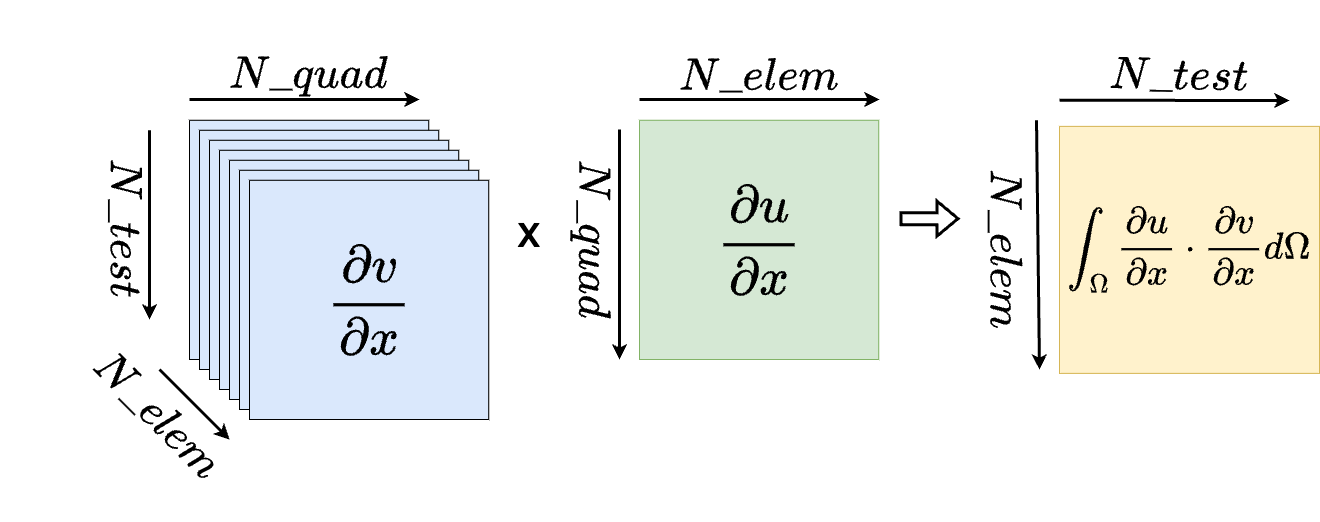
FastVPINNs computes the variational loss (9) by stacking the test functions and their gradients into a three-dimensional tensor and reshaping the neural network gradients into a matrix, see Figure 1, thus enabling the calculation of the final residual vector for all elements in a single operation using BLAS routines available in TensorFlow Abadi et al. (2015). This approach has two main advantages: using BLAS operations on the GPU allows for efficient and fast calculations, and stacking the gradients and performing tensor-based operations enable the loss for the entire domain to be computed in a single calculation, reducing the training time’s dependency on the number of elements, which is a major challenge in conventional hp-VPINNs frameworks. Additionally, FastVPINNs can handle complex geometries, making this method suitable for a wide range of problems. For further details on the implementation of the FastVPINNs framework, see Anandh et al. (2024a).
3 Loss Functional
The main topic of Frerichs-Mihov et al. (2024a) is the investigation of different loss functionals for PINNs and hp-VPINNs applied to the numerical solution of convection-dominated CDR problems. The motivation for studying different loss functionals stems from the observation that the standard residual is not an appropriate choice for performing parameter optimization in stabilized finite element methods, see John et al. (2011). It was observed in Frerichs-Mihov et al. (2024a) that it was possible to obtain more accurate solutions with loss functionals that are different to the standard residual loss.
In the current paper, two alternative loss functionals will be studied.
3.1 SUPG Stabilization Loss
The SUPG finite element method, which is already mentioned in the introduction, adds an additional term to the standard Galerkin finite element discretization. This term essentially introduces numerical diffusion in streamline direction. The global SUPG stabilization term has the form
| (10) |
where is called stabilization parameter and the diffusive term is neglected in the residual (the first factor), which is appropriate in the convection-dominated regime. In the framework of finite elements, (10) is localized by decomposing the integral in a sum of integrals over the mesh cells and then is often defined to be a piecewise constant function on the given triangulation. In the framework of neural networks, the SUPG stabilization loss functional is given by
| (11) |
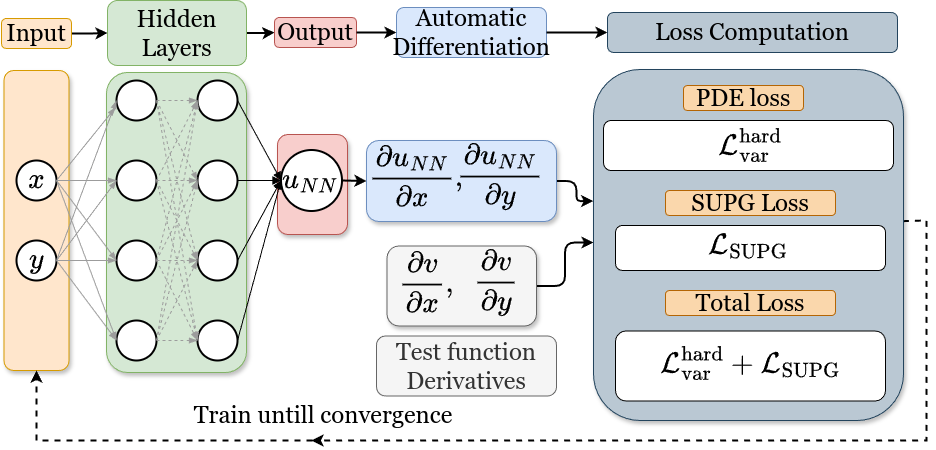
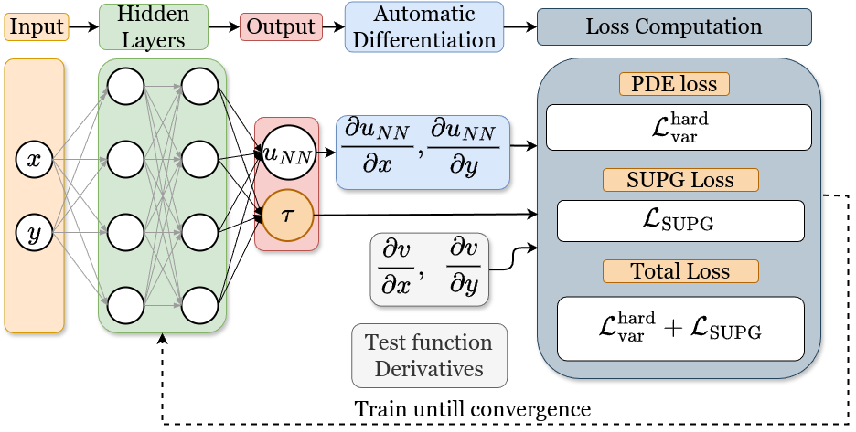
where is the variational loss defined in (9). Minimizing the loss functional (11) penalizes large streamline derivatives. Hence, the additional SUPG loss can be also interpreted as a physics-informed regularization term, since functions with small residuals but large streamline derivatives are excluded from the set of possible solutions. It is well known that regularization techniques might help to prevent overfitting. An architecture of the network for the loss functional including the SUPG term with prescribed stabilization parameter is presented in Figure 2.
3.2 Weight Regularization Loss
The training of a neural network requires the solution of a large-scale non-convex optimization problem. For such problems, usually a regularization term is included in the loss functional. In addition, this term might counteract overfitting and thus it enhances the generalization capacity of the network. A standard approach consists in adding a -type regularization, so that the loss functional becomes
| (12) |
where is the total number of entries in the weight matrices of the network and is the set of all weights in the network. The weight decay regularization parameter needs to be tuned.
4 Numerical Studies with Constant Parameters
In this section, we first validate the FastVPINNs code by solving the Eriksson–Johnson problem, as presented in Sikora et al. (2023), by comparing accuracy and computing times. Subsequently, we address two convection-dominated problems, assessing the performance of the proposed loss functionals (11) and (12) with constant stabilization and regularization parameter, respectively, within the framework of hp-VPINNs and we compare the results and efficiency with those reported in the literature.
All simulations were conducted on a system equipped with an AMD Threadripper CPU and an NVIDIA A6000 GPU. For neural network training, we utilized TensorFlow 2.0, specifically employing the tf.float64 datatype to ensure high precision. The network architecture incorporates tanh activation functions, and we used the Adam optimizer for the training iterations. We adopted test functions similar to those described in Kharazmi et al. (2021). These functions are defined as , where represents the th order Legendre polynomial. For numerical integration, we implemented Gauss–Lobatto–Legendre quadrature routines as used in Kharazmi et al. (2021).
4.1 Studied Problems
The Eriksson–Johnson Problem ()
This problem, originally proposed in Eriksson and Johnson (1991), was used in Sikora et al. (2023) for assessing a PINN for (mildly) convection-dominated problems. It is defined by , , , and the right-hand side of (1) is chosen such that the solution has the form
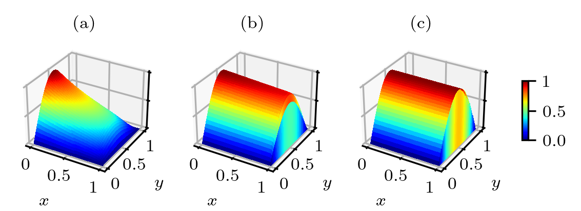
Dirichlet conditions were imposed on . Solutions for various values of the diffusion coefficient are displayed in Figure 3. The smallest value of the diffusion coefficient considered in Sikora et al. (2023) is . For small values of the diffusion coefficient, the solution exhibits a boundary layer at .
Solution with Outflow Boundary Layers ()
This example, proposed in John et al. (1997), features two layers at the outflow boundary, which, according to an asymptotic analysis, have a width of . The data for problem (1) are given by , , , , and the prescribed solution has the form:
| (13) | ||||
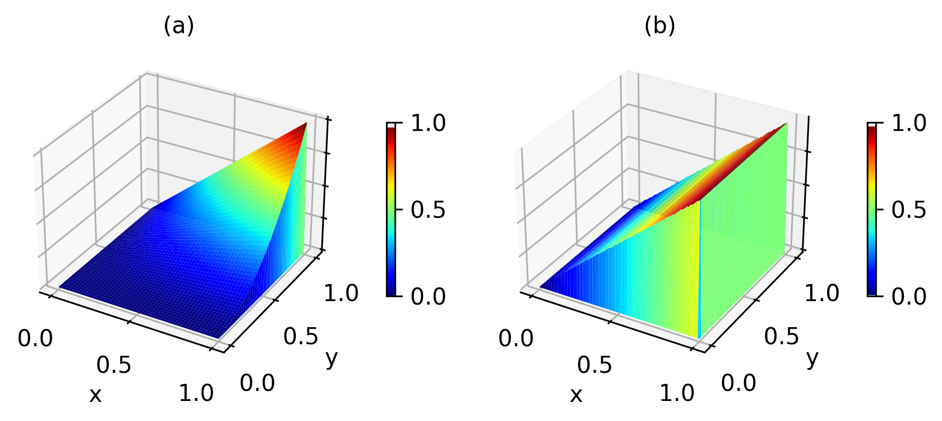
Dirichlet boundary conditions are imposed on . By construction, the outflow boundary layers are situated at and at , and there is even a so-called corner singularity at the right upper corner of the domain. Figure 4(a) depicts the prescribed solution (13).
Parabolic layer problem ()
The data for problem (1) are given by , , , , and . Homogeneous Dirichlet conditions are prescribed at . The solution exhibits an exponential layer at the outflow boundary and two parabolic boundary layers at the characteristic boundaries and , as shown in Figure 4 (b).
To obtain a high accuracy solution for this problem to compare with, we employed the Monotone Upwind-type Algebraically Stabilized (MUAS) method. The MUAS method, formulated in John and Knobloch (2022), is an algebraically stabilized scheme. It has been shown in the survey Barrenechea et al. (2024) that algebraically stabilized scheme are currently the most promising finite element approaches for computing solutions of convection-dominated convection-diffusion-reaction problems that satisfy Discrete Maximum Principles.
4.2 Validation of the FastVPINNs Implementation and Comparison with the Literature
In this section, we consider the Eriksson–Johnson problem as studied in Sikora et al. (2023) and compare the available data with our results. The approach in Sikora et al. (2023) utilizes a single element with 6400 quadrature points and a weak boundary constraint for the Dirichlet boundaries. In contrast, our hp-VPINNs method employs an element domain with test functions and quadrature points per element, i.e., in total also 6400 quadrature points, and it uses a hard boundary constraint for imposing Dirichlet conditions. Despite these differences, both approaches share common features in their neural network architecture and training process. Specifically, both use a neural network with hidden layers and neurons per hidden layer, employ the Adam optimizer for training with a learning rate of , and run for training epochs. In this study, we have used , as it was done in Sikora et al. (2023).
The indicator functions for the hard constraints (6) were chosen to be
with and . That means, for the indicator function we prescribed a sharp boundary layer at the boundary to account for the corresponding layer of the solution. This is not necessary at the other parts of the boundary. The standard loss functional defined in (9), which takes into account the hard constraint boundary conditions, was used.
| quadrature points | FastVPINNs | Sikora et al. (2023) | |
| 6400 | 0.1 | 0.265 | |
| 6400 | 0.01 | 0.346 | |
| 6400 | 0.001 | 0.332 |
| FastVPINNs (CPU) | FastVPINNs (GPU) | (Sikora et al., 2023, Fig. 14) |
| 0.011 | 0.0027 | 0.0375 |
Tables 1 and 2 present the obtained results. It can be seen that, on the one hand, the application of FastVPINNs gives results that are more accurate by several orders of magnitude than the results from Sikora et al. (2023). Here, the approximation of the error in is defined by
| (14) |
where is the number of test points at which the error is calculated. In all of the examples, the test points are given by a grid of equidistant points in . And on the other hand, the training times are considerably smaller, by a factor of about 3 on CPUs and by a factor of 14 if GPUs are used.
The obtained results validate our implementation of FastVPINNs. In our opinion, the improved accuracy compared with the literature can be attributed to two factors. First, the use of hard constraints for the boundary conditions, which seems to be essential for boundary layer problems, and second the -refinement approach of hp-VPINNs.
4.3 Studies with the SUPG Stabilization and the Regularization with Constant Parameters
In this section, we analyze the performance of the SUPG-based loss functional and loss functional with regularization applied to problems and . Concretely, our studies explore the SUPG stabilization defined in (11) and PDE loss with regularization given in (12). For the simulations, we employed a neural network architecture consisting of seven hidden layers with 30 neurons each. The domain was discretized into 64 cells, with 100 quadrature points and 36 test functions per cell, resulting in a total of 6400 quadrature points. To conduct the experiments, learning rates of and have been used. The is calculated as given in (14). The network is trained for 100,000 epochs, and the smallest error obtained during this training, i.e., after each epoch and not necessarily after the final epoch, is reported below. The used parameters are similar to those used in the studies described in Frerichs-Mihov et al. (2024a). For both problems, we applied an indicator function as presented in Frerichs-Mihov et al. (2024a):
| (15) |
| loss | search range | optimal value | |
| loss | search range | optimal value | |
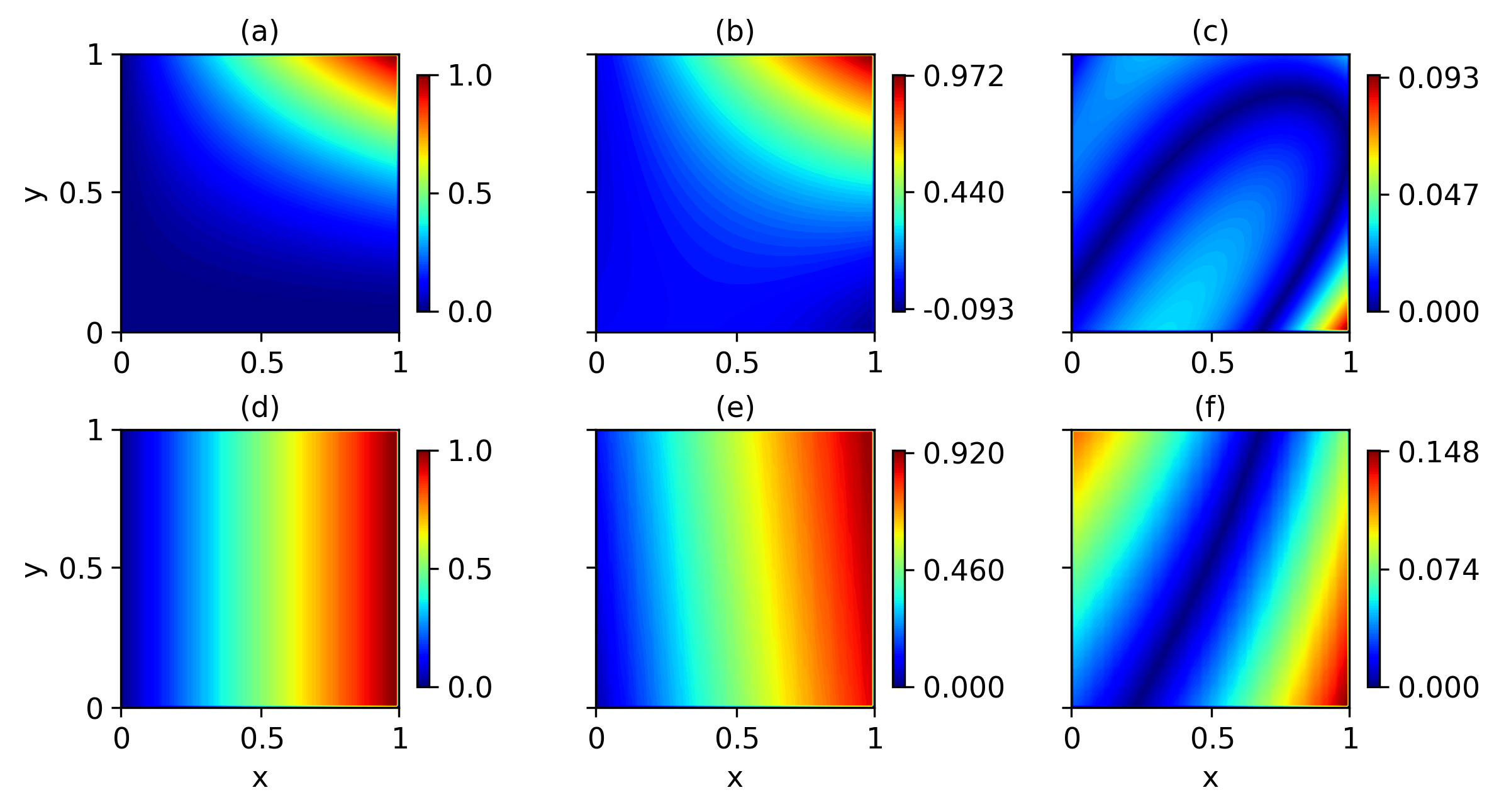
Our numerical studies were conducted in two phases. First, we performed an initial broad-range hyperparameter search, computing for a wide range of hyperparameters, as detailed in Tables 3 and 4. Following this, we conducted a refined hyperparameter search based on the best performing values from the initial search. The optimal hyperparameters for each loss functional are presented in aforementioned tables and the corresponding solutions and point-wise errors in Figure 5. For both problems, it can be seen that the SUPG stabilization () outperformed the approach that uses only regularization (). In particular, for problem our methods achieved lower errors compared to the PINNs and hp-VPINNs simulations performed in Frerichs-Mihov et al. (2024a). However, on the other hand, both results are not yet completely satisfactory. There is a comparatively big error in the right lower corner of the domain for the numerical solution of and the contour lines of the numerical solution of are not parallel to the -axis. But all in all, we think that the obtained results demonstrate that including the SUPG stabilization term is an appropriate way for enhancing the accuracy of variational physics-informed neural networks.
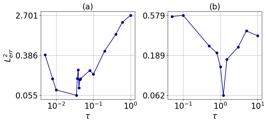
Next, results of a sensitivity analysis concerning the accuracy of the numerical solutions for variations of the parameter in will be presented. It is important to note that even when all parameters are kept constant, the minimum error obtained varies noticeably across multiple runs of the simulations. To obtain a more representative picture, we repeated the simulations 5 times and used the average of the minimum errors to plot the values shown in Figure 6. It is important to clarify that the errors mentioned in Tables 3 and 4 are the result of the best run only. For , it can be seen that there is a certain, but relatively small, interval for the stabilization parameter where the obtained errors are close to the best one. In the case of , there is even just a single stabilization parameter that gives the by far most accurate result. The best values from Figure 6 correspond with those from Tables 3 and 4. This study shows that a refined search is needed to find the optimal value of the stabilization parameter to obtain accurate results. This search is usually not feasible in practice since the solution of the problem is usually not known.
5 Learning the Parameters in the SUPG Loss and the Indicator Function
The studies from Section 4 and further preliminary numerical simulations have identified two main challenges in addressing convection-dominated CDR problems with the hp-VPINNs as studied in this paper. The first challenge consists in determining the optimal, or at least a good, SUPG stabilization parameter . The second challenge involves the choice of a suitable indicator function (7) for enforcing Dirichlet boundary conditions, see also Matthaiou et al. (2024) for a discussion of this challenge. This second challenge is particularly important because the indicator function must not only match the Dirichlet boundary values at the boundary, but its gradient near the boundary should also fit to the solution’s gradient. To address these challenges, we propose two enhancements to hp-VPINNs, and with that in particular to FastVPINNs. Firstly, we introduce a modified neural network that simultaneously predicts a spatially varying stabilization parameter along with the solution as shown in Figure 7. Secondly, we also propose an adaptive indicator function whose slope near the boundaries is controlled by a learnable parameter, which is learnt during the training process.
5.1 Neural Network Predicting the Stabilization Parameter
The stabilization parameter that controls the artificial streamline diffusion can be expressed as a function of the coefficients of the CDR problem and the local mesh width, as it is done in finite element methods. However, the difficulty of this approach is that the optimal stabilization parameter is not known for problems defined in two- and higher-dimensional domains. In a neural network context, the stabilization parameter can be considered as an additional hyperparameter that has to be found by performing hyperparameter tuning, as it was done in Section 4. However, this approach is time-consuming and it might be infeasible in practice.
To address this challenge, we propose a neural network that can predict the stabilization parameter along with the solution, as shown in Figure 7. With this approach, the neural network-predicted can be spatially varying, and this variation depends not only on the coefficients of the problem but also on the local shape of the predicted solution. This feature can also be observed for optimized SUPG stabilization parameters, e.g., see John et al. (2011, 2023). In this way, numerical stabilization is added only where needed.
The network-predicted is constrained using a sigmoid activation function to ensure that it remains positive. Preliminary numerical studies showed that it is of advantage, for obtaining consistent values of across different runs, to set to zero at the boundary of the domain. That means, the quadrature nodes on do not contribute to the SUPG stabilization loss defined in (10). In fact, the solution on is known and applying a stabilization there is not mandatory. We used the indicator function
where, is the stabilization parameter predicted by the neural network, is the sigmoid function, and is an indicator function defined by
Then we set
where , termed as ‘ growth’, is controlling the strength of the stabilization factor. The hyperparameter needs to be fine-tuned. The predicted is then used in the calculation of given in (11).
We will use problems and to demonstrate the effect of applying the learnt in the SUPG stabilization loss. Three approaches will be compared: PDE loss (9) only, PDE loss with SUPG stabilization (11) and constant , and PDE loss with SUPG stabilization (11) with learnt -based SUPG stabilization.
In our previous studies we observed that using a symmetric indicator function as given in (15) might generate large errors on the boundary when there is no steep gradient in the solution, compare Figure 5. Therefore, for this study, we applied a modified indicator function that has a steep slope at the outflow boundaries and and a low slope at the other two boundaries:
| (16) |
Similarly for , we applied a modified indicator function, which has a steep slope at boundaries , and , and a low slope at the boundary :
| (17) |
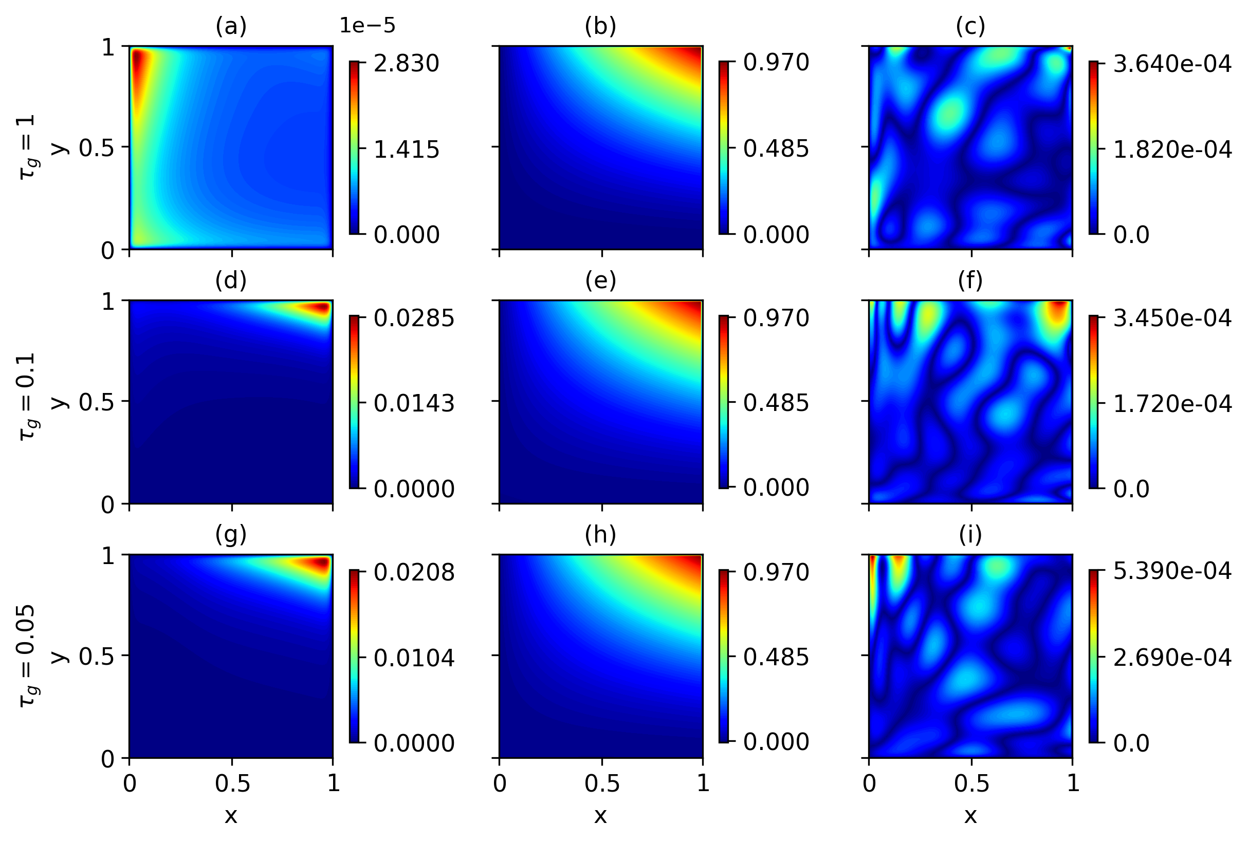
A neural network with seven hidden layers and 30 neurons per layer was used. The network was trained for epochs with a learning rate of . We used cells with quadrature points and test functions per cell. To determine the optimal hyperparameters for the constant and neural network-predicted , we initially performed a single run for each hyperparameter within the broad search ranges specified in Tables 5 and 6 for the problems and , respectively. From these initial runs, we identified the hyperparameters that performed the best for each approach. Subsequently, we ran 10 simulations using these optimal hyperparameters for each study. The average values from these 10 runs are presented in Tables 5 and 6. It can be observed that the model with the learnt (with the hyperparameter ) leads to notably more accurate results than both the model with constant (as a hyperparameter) and the model without any SUPG loss. Some representative solutions for the approach with the learnt stabilization parameter are presented in Figures 8 and 9.
| loss |
|
|
|||||
| search range | - | ||||||
| optimal parameter | - | ||||||
| best |
| loss |
|
|
|||||
| search range | - | ||||||
| optimal parameter | - | ||||||
| best |
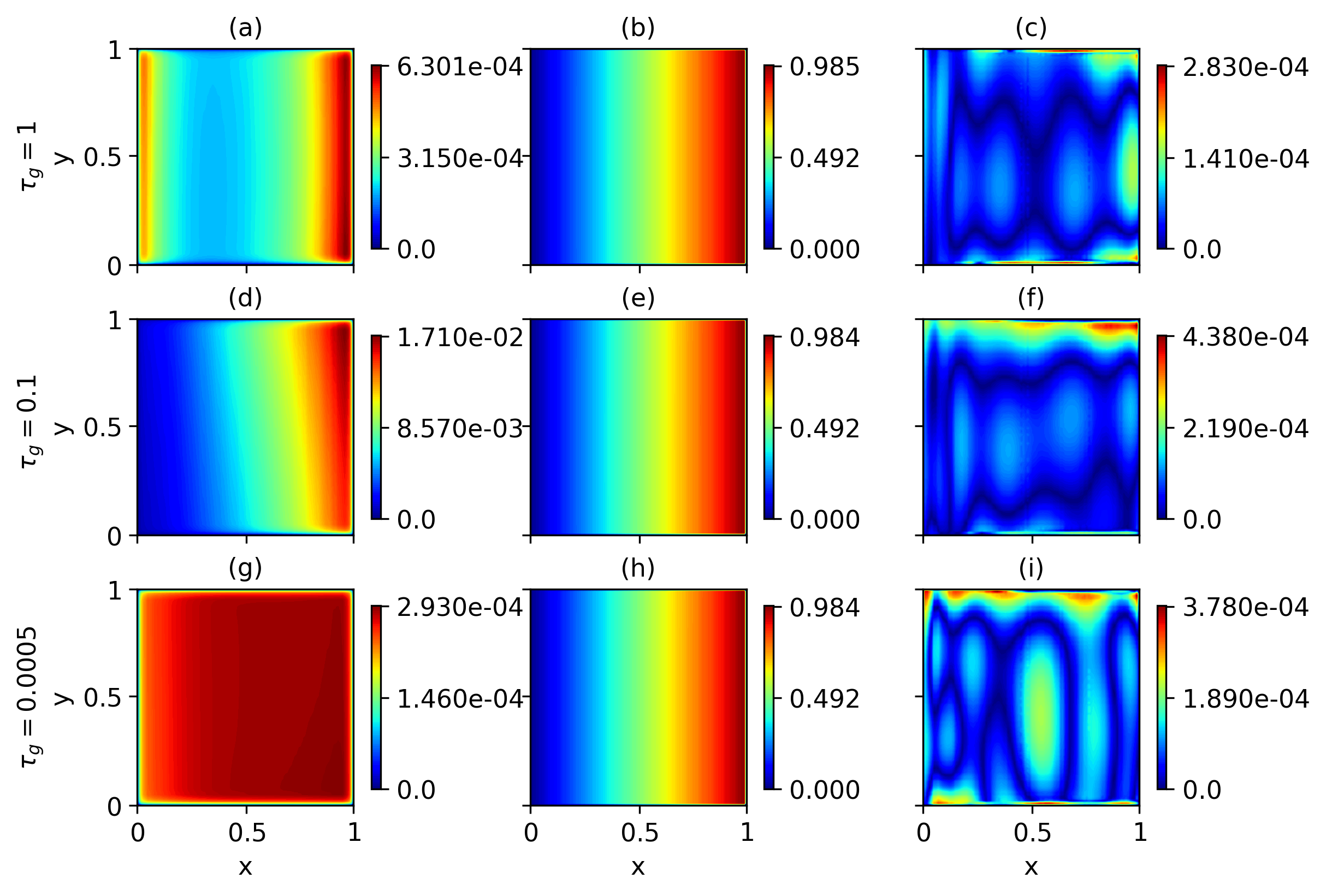
All errors presented in Tables 5 and 6 are considerably smaller than those in Tables 3 and 4, respectively. For , in particular the error in the right lower corner of the domain almost disappeared, compare Figures 5 and 8. In the case of , the contour lines of the computed solutions are parallel to the -axis now. These observations show that a combination of a learnt stabilization parameter and a suitable indicator function, namely using (16) and (17) instead of (15), leads to a tremendous increase of accuracy.
5.2 Adaptive Indicator Function
In our previous set of studies, we used a fixed indicator function to impose hard-constrained boundary conditions and we observed in preliminary simulations that the choice of the indicator function might have a considerable impact on the accuracy of the computed solutions. To the best of our knowledge, there is no proposal available on how to select a priori a good indicator function. That’s why, we pursue an approach to compute an adaptive indicator function. This function is still of the same principal form as used so far, but it is constructed using trainable parameters that control the slope of the function near the boundaries. Our approach will enable the neural network to learn not only the solution but also the parameters for the indicator functions, resulting in a better fit for the specific parameters of the chosen problem.
Concerning problem , we propose an adaptive indicator function of form (18), more precisely,
| (18) |
where and are learnable parameters controlling the gradient near the boundaries. Specifically, governs the behavior at the inlet boundaries, while controls the behavior at the outflow boundaries.
Similarly, we introduce an adaptive indicator function for with three learnable parameters: , , and , namely
| (19) |
In this formulation, affects the inlet boundary, the characteristic boundaries, and the outflow boundary.
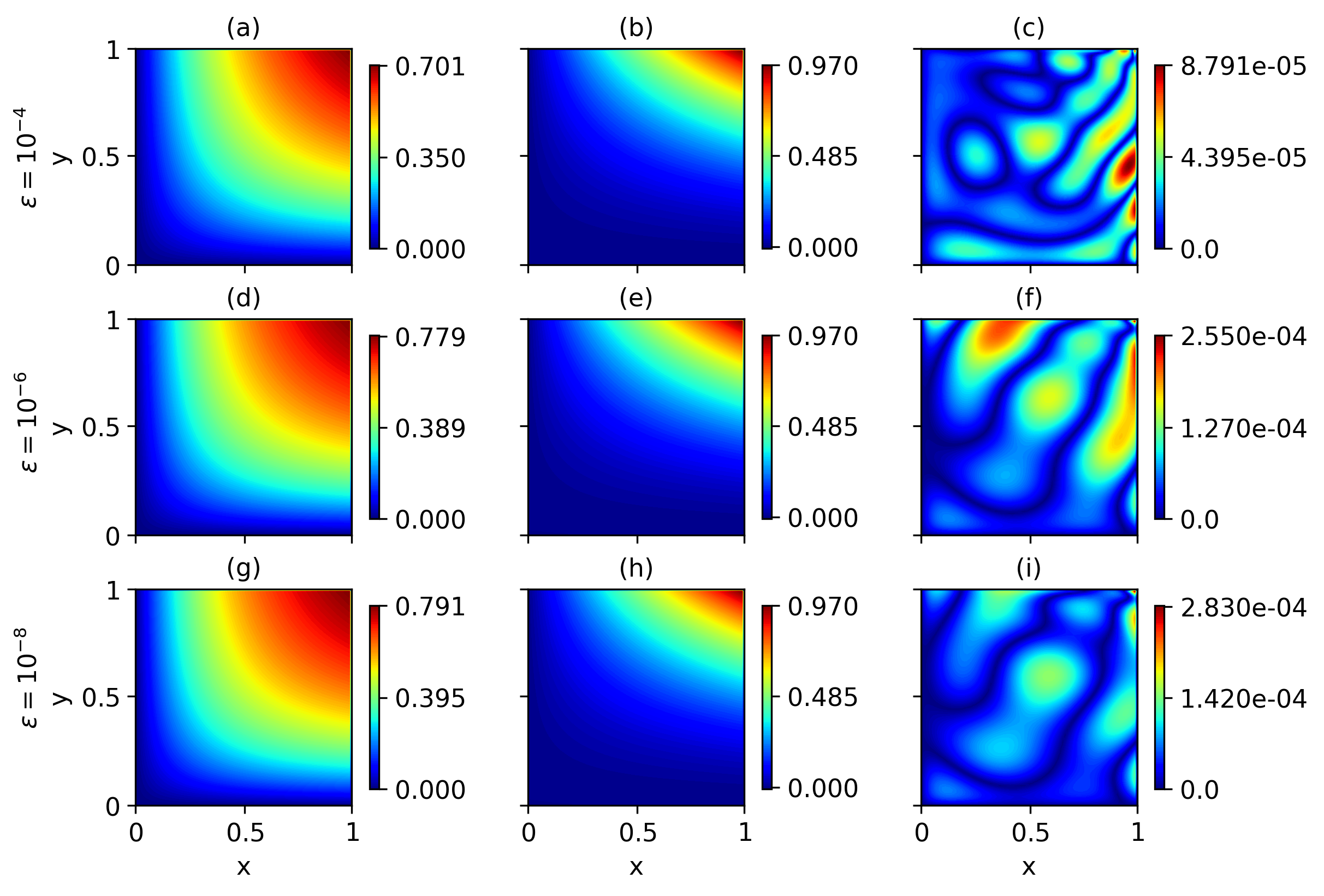
The numerical studies with adaptive indicator functions were performed only with the loss functional from (9). Since the steepness of layers depends on the Péclet number, we considered different values of the diffusion coefficient to investigate how the network’s prediction of the indicator function depends on the steepness of the layers.
|
|
|
|
|
|
|||||||||||||
Results for are presented in Figure 10 and Table 7. The parameters for the indicator function were initialized with and , where . For instance, when , we set . It can be seen in Table 7 that in fact very different parameters are proposed by the neural network for the inlet and outflow boundaries, respectively, with the value at the inlet boundaries being considerably smaller. The parameters do not depend very much on the diffusion coefficient, i.e., on the Péclet number. The indicator functions have a different shape than the function given in (16), which takes values very close to 1 in most parts of . It can be seen that the results obtained with the adapted parameters are (much) more accurate than those with the initial parameters. Comparing with Table 5, one can notice also that the error in the case is noticeably smaller if the adaptive indicator function is used.
|
|
|
|
|
|
|
|
|||||||||||||||||
| 1 | 2.129 | 0 | -0.086 | 2 | 3.927 | |||||||||||||||||||
| 1 | 3.295 | 0 | -0.088 | 3 | 3.921 | |||||||||||||||||||
| 2 | 3.380 | 0 | -0.079 | 4 | 4.004 |
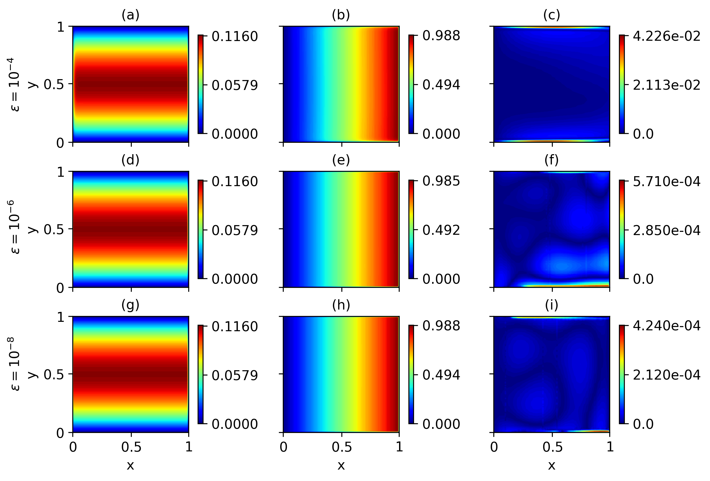
For problem , whose solution possesses different types of layers and whose ansatz for the indicator function is given in (19), the obtained results are given in Figure 11 and Table 8. The evaluation comes to similar conclusions as for the other example. Again, the learnt parameters for the indicator function depend only slightly on the Péclet number. The visualizations of the indicator functions look very much alike. Comparing with Table 6, one can observe that the results for is considerably more accurate for the approach with adaptive indicator function.
6 Conclusion
FastVPINNs are a very efficient approach for computing approximations of solutions of boundary value problems. In this paper, this approach was combined with two methods for improving the accuracy of computed solutions of convection-diffusion-reaction problems in the convection-dominated regime. First, the residual loss was augmented with a SUPG stabilization term and an architecture was proposed that computes a spatially varying stabilization parameter. And second, an architecture was developed that learns appropriate parameters for defining a good indicator function for imposing hard-constrained Dirichlet boundary conditions. Both extensions led to a considerable increase of the accuracy of the computed solutions. In contrast, the inclusion of a regularization term with the weights of the network was not helpful for obtaining solutions with higher accuracy.
References
- Abadi et al. (2015) Martín Abadi, Ashish Agarwal, Paul Barham, Eugene Brevdo, Zhifeng Chen, Craig Citro, Greg S. Corrado, Andy Davis, Jeffrey Dean, Matthieu Devin, Sanjay Ghemawat, Ian Goodfellow, Andrew Harp, Geoffrey Irving, Michael Isard, Yangqing Jia, Rafal Jozefowicz, Lukasz Kaiser, Manjunath Kudlur, Josh Levenberg, Dandelion Mané, Rajat Monga, Sherry Moore, Derek Murray, Chris Olah, Mike Schuster, Jonathon Shlens, Benoit Steiner, Ilya Sutskever, Kunal Talwar, Paul Tucker, Vincent Vanhoucke, Vijay Vasudevan, Fernanda Viégas, Oriol Vinyals, Pete Warden, Martin Wattenberg, Martin Wicke, Yuan Yu, and Xiaoqiang Zheng. TensorFlow: Large-scale machine learning on heterogeneous systems, 2015. URL https://www.tensorflow.org/. Software available from tensorflow.org.
- Abueidda et al. (2021) Diab W. Abueidda, Qiyue Lu, and Seid Koric. Meshless physics-informed deep learning method for three-dimensional solid mechanics. Internat. J. Numer. Methods Engrg., 122(23):7182–7201, 2021. ISSN 0029-5981,1097-0207.
- Anandh et al. (2024a) Thivin Anandh, Divij Ghose, and Sashikumaar Ganesan. FastVPINNs: An efficient tensor-based Python library for solving partial differential equations using hp-Variational Physics Informed Neural Networks. Journal of Open Source Software, 9(99):6764, 2024a.
- Anandh et al. (2024b) Thivin Anandh, Divij Ghose, Himanshu Jain, and Sashikumaar Ganesan. FastVPINNs: Tensor-Driven Acceleration of VPINNs for Complex Geometries. arXiv preprint arXiv:2404.12063, 2024b.
- Baker et al. (2019) Nathan Baker, Frank Alexander, Timo Bremer, Aric Hagberg, Yannis Kevrekidis, Habib Najm, Manish Parashar, Abani Patra, James Sethian, Stefan Wild, Karen Willcox, and Steven Lee. Workshop report on basic research needs for scientific machine learning: Core technologies for artificial intelligence. USDOE Office of Science (SC), Washington, D.C. (United States), 2 2019. doi: 10.2172/1478744. URL https://www.osti.gov/biblio/1478744.
- Barrenechea et al. (2024) Gabriel R. Barrenechea, Volker John, and Petr Knobloch. Finite element methods respecting the discrete maximum principle for convection-diffusion equations. SIAM Rev., 66(1):3–88, 2024. ISSN 0036-1445,1095-7200.
- Brooks and Hughes (1982) Alexander N. Brooks and Thomas J. R. Hughes. Streamline upwind/Petrov-Galerkin formulations for convection dominated flows with particular emphasis on the incompressible Navier-Stokes equations. Comput. Methods Appl. Mech. Engrg., 32(1-3):199–259, 1982. ISSN 0045-7825. FENOMECH ’81, Part I (Stuttgart, 1981).
- Cuomo et al. (2022) Salvatore Cuomo, Vincenzo Schiano Di Cola, Fabio Giampaolo, Gianluigi Rozza, Maziar Raissi, and Francesco Piccialli. Scientific machine learning through physics-informed neural networks: where we are and what’s next. J. Sci. Comput., 92(3):Paper No. 88, 62 pages, 2022. ISSN 0885-7474,1573-7691.
- Eriksson and Johnson (1991) Kenneth Eriksson and Claes Johnson. Adaptive finite element methods for parabolic problems. I: A linear model problem. SIAM J. Numer. Anal., 28(1):43–77, 1991. ISSN 0036-1429.
- Frerichs-Mihov et al. (2024a) Derk Frerichs-Mihov, Linus Henning, and Volker John. On loss functionals for physics-informed neural networks for steady-state convection-dominated convection-diffusion problems. Comm. Appl. Math. Comp., page to appear, 2024a.
- Frerichs-Mihov et al. (2024b) Derk Frerichs-Mihov, Volker John, and Marwa Zainelabdeen. On collocation points for physics-informed neural networks applied to convection-dominated convection-diffusion problems. In Proceedings of ENUMATH 2023. Springer, 2024b. accepted.
- Ganesan and Tobiska (2017) Sashikumaar Ganesan and Lutz Tobiska. Finite elements. Cambridge-IISc Series. Cambridge University Press, Cambridge, 2017. ISBN 978-1-108-41570-5. Theory and algorithms.
- Ghose et al. (2024) Divij Ghose, Thivin Anandh, and Sashikumaar Ganesan. FastVPINNs: A fast, versatile and robust Variational PINNs framework for forward and inverse problems in science. In ICLR 2024 Workshop on Differential Equations in Science, 2024.
- Hughes and Brooks (1979) T. J. R. Hughes and A. Brooks. A multidimensional upwind scheme with no crosswind diffusion. In Finite element methods for convection dominated flows (Papers, Winter Ann. Meeting Amer. Soc. Mech. Engrs., New York, 1979), volume 34 of AMD, pages 19–35. Amer. Soc. Mech. Engrs. (ASME), New York, 1979.
- John et al. (1997) V. John, J. M. Maubach, and L. Tobiska. Nonconforming streamline-diffusion-finite-element-methods for convection-diffusion problems. Numer. Math., 78(2):165–188, 1997. ISSN 0029-599X.
- John and Knobloch (2007) Volker John and Petr Knobloch. On spurious oscillations at layers diminishing (SOLD) methods for convection-diffusion equations. I. A review. Comput. Methods Appl. Mech. Engrg., 196(17-20):2197–2215, 2007. ISSN 0045-7825.
- John and Knobloch (2022) Volker John and Petr Knobloch. On algebraically stabilized schemes for convection-diffusion-reaction problems. Numer. Math., 152(3):553–585, 2022. ISSN 0029-599X,0945-3245.
- John et al. (2011) Volker John, Petr Knobloch, and Simona B. Savescu. A posteriori optimization of parameters in stabilized methods for convection-diffusion problems—Part I. Comput. Methods Appl. Mech. Engrg., 200(41-44):2916–2929, 2011. ISSN 0045-7825.
- John et al. (2023) Volker John, Petr Knobloch, and Ulrich Wilbrandt. A posteriori optimization of parameters in stabilized methods for convection-diffusion problems—Part II. J. Comput. Appl. Math., 428:Paper No. 115167, 17 pages, 2023. ISSN 0377-0427,1879-1778.
- Kharazmi et al. (2019) Ehsan Kharazmi, Zhongqiang Zhang, and George Em Karniadakis. Variational physics-informed neural networks for solving partial differential equations. arXiv preprint arXiv:1912.00873, 2019.
- Kharazmi et al. (2021) Ehsan Kharazmi, Zhongqiang Zhang, and George E. M. Karniadakis. -VPINNs: variational physics-informed neural networks with domain decomposition. Comput. Methods Appl. Mech. Engrg., 374:Paper No. 113547, 25 pages, 2021. ISSN 0045-7825,1879-2138.
- Khodayi-Mehr and Zavlanos (2020) Reza Khodayi-Mehr and Michael Zavlanos. Varnet: Variational neural networks for the solution of partial differential equations. In Learning for Dynamics and Control, pages 298–307. PMLR, 2020.
- Krishnapriyan et al. (2021) Aditi Krishnapriyan, Amir Gholami, Shandian Zhe, Robert Kirby, and Michael W Mahoney. Characterizing possible failure modes in physics-informed neural networks. In Advances in Neural Information Processing Systems, volume 34, pages 26548–26560, Virtual, Online, 2021. Curran Associates, Inc.
- Lagaris et al. (1998) I.E. Lagaris, A. Likas, and D.I. Fotiadis. Artificial neural networks for solving ordinary and partial differential equations. IEEE Transactions on Neural Networks, 9(5):987–1000, 1998.
- Lu et al. (2021a) Lu Lu, Xuhui Meng, Zhiping Mao, and George Em Karniadakis. DeepXDE: a deep learning library for solving differential equations. SIAM Rev., 63(1):208–228, 2021a. ISSN 0036-1445,1095-7200.
- Lu et al. (2021b) Lu Lu, Raphaël Pestourie, Wenjie Yao, Zhicheng Wang, Francesc Verdugo, and Steven G. Johnson. Physics-informed neural networks with hard constraints for inverse design. SIAM J. Sci. Comput., 43(6):B1105–B1132, 2021b. ISSN 1064-8275,1095-7197.
- Matthaiou et al. (2024) Marina Matthaiou, Volker John, and Marwa Zainelabdeen. Bound-preserving PINNs for steady-state convection-diffusion-reaction problems. WIAS Preprint No. 3134, 2024.
- (28) NVIDIA Modulus, 2024. https://developer.nvidia.com/modulus. Last accessed Jan 01, 2024.
- Psaros et al. (2023) Apostolos F. Psaros, Xuhui Meng, Zongren Zou, Ling Guo, and George Em Karniadakis. Uncertainty quantification in scientific machine learning: methods, metrics, and comparisons. J. Comput. Phys., 477:Paper No. 111902, 83 pages, 2023. ISSN 0021-9991,1090-2716.
- Raissi et al. (2019) M. Raissi, P. Perdikaris, and G. E. Karniadakis. Physics-informed neural networks: a deep learning framework for solving forward and inverse problems involving nonlinear partial differential equations. J. Comput. Phys., 378:686–707, 2019. ISSN 0021-9991,1090-2716.
- Roos et al. (2008) Hans-Görg Roos, Martin Stynes, and Lutz Tobiska. Robust numerical methods for singularly perturbed differential equations, volume 24 of Springer Series in Computational Mathematics. Springer-Verlag, Berlin, second edition, 2008. ISBN 978-3-540-34466-7. Convection-diffusion-reaction and flow problems.
- Sikora et al. (2023) Maciej Sikora, Patryk Krukowski, Anna Paszynska, and Maciej Paszynski. Physics informed neural networks with strong and weak residuals for advection-dominated diffusion problems, 2023.
- Yadav and Ganesan (2024) Sangeeta Yadav and Sashikumaar Ganesan. Artificial neural network-augmented stabilized finite element method. J. Comput. Phys., 499:Paper No. 112702, 15 pages, 2024. ISSN 0021-9991,1090-2716.