A Flexible Framework for Grant-Free Random Access in Cell-Free Massive MIMO Systems

Abstract

We propose a novel generalized framework for grant-free random-access (GFRA) in cell-free massive multiple-input multiple-output systems where multiple geographically separated access points (APs) or base stations (BSs) aim to detect sporadically active user-equipment (UEs). Unlike a conventional architecture in which all the active UEs transmit their signature or pilot sequences of equal length, we admit a flexible pilot length for each UE, which also enables a seamless integration into conventional grant-based wireless systems. We formulate the joint UE activity detection and the distributed channel estimation as a sparse support and signal recovery problem, and describe a Bayesian learning procedure to solve it. We develop a scheme to fuse the posterior statistics of the latent variables inferred by each AP to jointly detect the UEs’ activities, and utilize them to further refine the channel estimates. In addition, we allude to an interesting point which enables this flexible GFRA framework to encode the information bits from the active UEs. We numerically evaluate the normalized mean square error and the probability of miss-detection performances obtained by the Bayesian algorithm and show that the latent-variable fusion enhances the detection and the channel estimation performances by a large margin. We also benchmark against a genie-aided algorithm which has a prior knowledge of the UEs’ activities.

I Introduction

Grant-free random-access (GFRA)or massive machine-type communication (MTC) is one of the potential technologies that is expected to play a crucial role in the next-generation wireless standards [1, 2]. With an increasing demand for several internet-of-things applications in the health, infrastructure, energy sectors, etc., and with a limited availability of wireless resources, obtaining a dedicated block of wireless resources to cater to a sporadically active set of user-equipment (UEs)may not always be feasible. Moreover, each MTC UE may not occupy a complete resource block (RB) of the same size as a conventional UE which may deem a typical multi-user multiple-input multiple-output (MIMO)receiver algorithm not an appropriate fit. Therefore, it is imperative to develop schemes which are flexible enough to be adapted to both the conventional and MTC communications.

Massive GFRA is a well researched topic where one or multiple access points (APs)attempt to detect sporadically active UEs using their transmitted uplink (UL) signature or pilot sequences, and a few of the relevant papers are [1, 2, 3, 4, 5, 6, 7, 8, 9, 10]. Typically, all the existing literature consider a system model where the active UEs transmit their pilot sequences of equal length, and the APs detect their activities and estimate their channel state information (CSI) using sparse signal recovery algorithms [11, 12, 13, 14]. However, to the best of our knowledge, none of the existing papers account for a scenario where the active UEs send their signature sequences of different lengths, which can potentially enable a seamless integration with the conventional grant-based wireless systems. This restriction of equal pilot lengths to the UEs can possibly narrow down the scope of GFRA in practical scenarios, especially when there is a resource crunch.

To broaden the realm and make GFRA appealing to be implemented in practice, we break the notion of equal pilot lengths for all the MTC UEs, and develop a generalized and a flexible framework in a distributed or cell-free massive multiple-input multiple-output (MIMO) setup. Therefore, we can fit the MTC UEs along with any other normal UEs which are allocated resources in a grant based manner. The size of the RB of a conventional UE can be interpreted as the transmission window in which the MTC UEs can send their pilot sequences of any size. We can see that this also subsumes a standard GFRA case when the transmission window is of the same size as the pilot length, which makes our structure general.

We propose a novel generalized massive GFRA framework where the MTC UEs can transmit their variable length signature sequences within a transmission window of a predefined size for activity detection and channel estimation. We formulate this as a distributed sparse signal and support recovery problem and adopt a Bayesian framework to solve it at the multiple distributed APs. Then, we devise a scheme to fuse the posterior statistics of the latent variables from the APs to improve the activity detection and channel estimation performance. We empirically evaluate the probability of miss-detection (MD)and the normalized mean square error (NMSE)performances of the developed algorithm, and benchmark against a genie-aided estimator which has a prior knowledge of the activities of the UEs.

We advert to another interesting point that can be utilized by this flexible framework to encode information bits depending on the sizes of the pilot sequence of a UE and the transmission window. For instance, if we denote the pilot length and the transmission window by $T$ and $W$, respectively, then we can encode $\lfloor\log_{2}\left(T-W+1\right)\rfloor$ information bits based on the occupancy of the pilot sequence within the transmission window. Therefore, this generalized structure not only seamlessly integrates into a conventional wireless system but also provides an additional benefit (almost for “free”), which makes it furthermore significant to design specialized and novel receiver algorithms.

II System Model and Problem Statement

We consider an UL cell-free massive MIMO wireless communication system with $L$ APs equipped with $N_{r}$ antennas each, receiving signals from $K$ out of $N$ ($K\ll N$) single transmit antenna UEs. We represent the channel between the $k$-th UE and the $\ell$-th AP by $\mathbf{b}_{\ell k}\in\mathbb{C}^{N_{r}\times 1}$ which follows a circularly symmetric complex normal distribution $\mathcal{CN}\left(\mathbf{b}_{\ell k};\mathbf{0},\beta_{\ell k}\mathbf{I}_{N_{r}}\right)$, where $\beta_{\ell k}$ is the large scale fading coefficient (LSFC). The APs do not have any prior information about the activity pattern of the UEs, i.e., they do not know the value of $K$. The $k$-th UE can potentially transmit its pilot signal of length $T_{k}$ symbols within an observation window of $W$ symbol intervals. We consider the case when the APs know the size of the transmission window and the lengths of the UEs’ pilot signals, but do not have any information about the exact starting symbol intervals of the UEs’ transmissions. We represent the received signal at the $\ell$-th AP during the $W$ symbol intervals as:

$$\mathbf{Z}_{\ell}^{T} =\sum_{k=1}^{K}\mathbf{b}_{\ell i_{k}}\begin{bmatrix}\underbrace{0,\ldots,0}_{S_{i_{k}}-1}&\mathbf{x}_{i_{k}}^{T}&\underbrace{0,\ldots,0}_{W-\left(T_{{i_{k}}}+S_{i_{k}}-1\right)}\end{bmatrix}+\mathbf{W}_{\ell}^{T},$$ (1)

where $\mathbf{Z}_{\ell}^{T}\in\mathbb{C}^{N_{r}\times W}$, $\ell\in\{1,\ldots,L\}$, $i_{k}\in\{1,\ldots,N\}$ denotes the index of the $k$-th active UE, $k\in\{1,\ldots,K\}$, ${\mathbf{x}_{i_{k}}}=\left[x_{{i_{k}},1},\ldots,x_{{i_{k}},T_{{i_{k}}}}\right]^{T}\in\mathbb{C}^{T_{{i_{k}}}\times 1}$, and $S_{i_{k}}\in\{1,\ldots,W-T_{{i_{k}}}+1\}$ are the pilots and the starting symbol index of the ${i_{k}}$-th active UE, respectively, $\mathbf{W}_{\ell}^{T}\in\mathbb{C}^{N_{r}\times W}$ is the additive noise with i.i.d. circularly symmetric complex Gaussian entries of mean $0$ and variance $1$. The maximum transmit power of each UE is $P_{\rm max}^{(\rm Tx)}$, i.e., $\mathbb{E}[\left\|\mathbf{x}_{k}\right\|^{2}]\leq P_{\rm max}^{(\rm Tx)}$, $k\in[1,\ldots,N]$.

Our goal is to develop a distributed algorithm that jointly detects the activity of the UEs and estimate their channels given the received signals $\mathbf{Z}_{\ell}$, $\ell\in[1,\ldots,L]$ and the pilot symbols $\mathbf{x}_{k}$, $k\in\{1,\ldots,N\}$. We rewrite (1) to formulate the device activity detection and channel estimation problem as follows:

$$\mathbf{Z}_{\ell}^{T} =\sum_{k=1}^{K}\begin{bmatrix}\mathbf{0}_{N_{r}\times\left(S_{i_{k}}-1\right)}&\mathbf{b}_{\ell i_{k}}&\mathbf{0}_{N_{r}\times\left(W-T_{i_{k}}-S_{i_{k}}+1\right)}\end{bmatrix}$$

$$\qquad\qquad\qquad\times\begin{bmatrix}\mathbf{x}_{i_{k}}^{T}&0&\ldots&0\\ \vdots&\vdots&\ddots&\vdots\\ 0&0&\ldots&\mathbf{x}_{i_{k}}^{T}\end{bmatrix}+\mathbf{W}_{\ell}^{T},$$ (2)

$$=\sum_{k=1}^{K}\mathbf{G}_{\ell i_{k}}^{T}\mathbf{D}_{i_{k}}^{T}+\mathbf{W}_{\ell}^{T},$$ (3)

where $\mathbf{G}_{\ell i_{k}}\in\mathbb{C}^{\left(W-T_{i_{k}}+1\right)\times N_{r}}$ contains one non-zero row ($S_{i_{k}}$-th row is non-zero), and $\mathbf{D}_{i_{k}}^{T}\in\mathbb{C}^{\left(W-T_{i_{k}}+1\right)\times W}$ contains the pilot sequences of the $i_{k}$-th UE. Now, when we include all the inactive devices into (3), we get

$$\mathbf{Z}_{\ell}^{T} =\sum_{k=1}^{N}\mathbf{G}_{\ell k}^{T}\mathbf{D}_{k}^{T}+\mathbf{W}_{\ell}^{T},$$ (4)

where $\mathbf{G}_{\ell k}\in\mathbb{C}^{\left(W-T_{k}+1\right)\times N_{r}}$ is non-zero only for the $K$ active UEs (which is unknown). We transpose (4) and rewrite in a matrix form as:

$$\mathbf{Z}_{\ell}=\mathbf{D}\mathbf{G}_{\ell}+\mathbf{W}_{\ell},\qquad\ell\in[1,\ldots,L],$$ (5)

where
$\mathbf{G}_{\ell}=\begin{bmatrix}\mathbf{G}_{\ell 1}^{T}&\ldots&\mathbf{G}_{\ell N}^{T}\end{bmatrix}^{T}\in\mathbb{C}^{\left((W+1)N-\sum_{k=1}^{N}T_{k}\right)\times N_{r}}$ is a joint row-sparse matrix with $K$ non-zero rows, and
$\mathbf{D}=\begin{bmatrix}\mathbf{D}_{1}&\ldots&\mathbf{D}_{N}\end{bmatrix}\in\mathbb{C}^{W\times\left((W+1)N-\sum_{k=1}^{N}T_{k}\right)}$ is the over-complete dictionary matrix.

Estimating $\mathbf{G}_{\ell}$ using the received signal $\mathbf{Z}_{\ell}$ is a local multiple-measurement-vector (MMV) sparse signal recovery problem at the $\ell$-th AP. Our aim is to use the received signals $\mathbf{Z}_{1},\ldots,\mathbf{Z}_{L}$ to jointly detect the active UEs and estimate the channels at each AP. Moreover, the support set of $\{\mathbf{G}_{1},\ldots,\mathbf{G}_{L}\}$ also determines the starting symbol times of the active UEs. For convenience, we denote the $n$-th column of $\mathbf{G}_{\ell}$ and $\mathbf{Z}_{\ell}$ as $\mathbf{g}_{\ell n}\in\mathbb{C}^{\left((W+1)N-\sum_{k=1}^{N}T_{k}\right)\times 1}$ and $\mathbf{z}_{\ell n}\in\mathbb{C}^{W\times 1}$, $n\in\{1,\ldots,N_{r}\}$, respectively, and $M\triangleq(W+1)N-\sum_{k=1}^{N}T_{k}$. Now, we describe the algorithm for the UE activity detection and distributed channel estimation.

III Sparse Bayesian Joint User Activity Detection and Distributed Channel Estimation

Our goal is to infer the posterior distributions of $\mathbf{G}_{\ell}$ given $\mathbf{Z}_{\ell}$ and $\mathbf{x}_{k}$, $k\in\{1,\ldots,N\}$, $\ell\in\{1,\ldots,L\}$. Each AP uses its local received signal to estimate its channel in a distributed fashion and a central processing unit (CPU) fuses the posterior statistics of the latent variables to jointly detect the active UEs. A key point to note is that the support set of $\mathbf{G}_{\ell}$, $\ell\in\{1,\ldots,L\}$, is common across all the APs, and we utilize this for the joint UE activity detection. We adopt the sparse-Bayesian-learning (SBL) or variational-Bayesian (VB) framework to infer the posterior distributions of the UEs’ channels locally at each AP, and then combine them to detect their activities at a CPU. We refer the reader to [11, 12, 13] for detailed descriptions of VB and SBL.

We describe the VB procedure here. To begin with, we impose a sparsity promoting two-stage hierarchical complex Gaussian prior on the columns of $\mathbf{G}_{\ell}$ with mean $\mathbf{0}$ and a common diagonal precision matrix $\mathbf{P}_{\ell}=\mathrm{diag}\left(\bm{\alpha}_{\ell}\right)$, where $\bm{\alpha}_{\ell}=\left[\alpha_{1},\ldots,\alpha_{M}\right]^{T}\in\mathbb{R}_{+}^{M\times 1}$. We treat the elements of $\bm{\alpha}_{\ell}$ as independent and identically distributed latent variables which follow a non-informative Gamma hyperprior with given rate and shape parameters. Such a two-stage hierarchical structure results in a Student’s $t$-distributed prior on $\mathbf{g}_{\ell n}$, $n\in\{1,\ldots,N_{r}\}$, $l\in\{1,\ldots,L\}$, which is heavy tailed and promotes sparse estimates.

III-A Distributed Channel Estimation

To obtain the posterior distributions of the channels via the VB procedure, we impose an independence structure on the latent variables $\mathbf{g}_{\ell n}$, $n\in\{1,\ldots,N_{r}\}$, and $\alpha_{\ell m}$, $m\in\{1,\ldots,M\}$, $\ell\in\{1,\ldots,L\}$, which means that the joint posterior probability distribution is the product of the posterior distributions of the individual latent variables. Then, we compute them to minimize the Kullback-Leibler (KL) divergence between the approximate and the original posterior distributions. We do not include the fundamentals of the VB or SBL framework due to lack of space. In VB, we decompose the natural logarithm of the joint probability distribution of the observations and the latent variables as follows:

$$\log P\left(\mathbf{Z}_{\ell},\mathbf{G}_{\ell},\bm{\alpha}_{\ell};{\mathbf{D}},a,b\right)$$

$$=\sum_{n=1}^{N_{r}}\log P_{\mathbf{z}_{\ell n}}\left(\mathbf{z}_{\ell n}\,\arrowvert\,\mathbf{g}_{\ell n};{\mathbf{D}}\right)+\sum_{n=1}^{N_{r}}\log P_{\mathbf{g}_{\ell n}}\left(\mathbf{g}_{\ell n}\,\arrowvert\,\bm{\alpha}_{\ell}\right)$$

$$\qquad\qquad\qquad\qquad+\sum_{m=1}^{M}\log P_{\alpha_{\ell m}}\left(\alpha_{\ell m};a,b\right),$$ (6)

where the conditional probability distributions are given by

$$P_{\mathbf{z}_{\ell n}}\left(\mathbf{z}_{\ell n}\,\arrowvert\,\mathbf{g}_{\ell n};{\mathbf{D}}\right)\propto\exp\left(-\left\|\mathbf{z}_{\ell n}-\mathbf{D}\mathbf{g}_{\ell n}\right\|^{2}\right),$$ (7)

$$P_{\mathbf{g}_{\ell n}}\left(\mathbf{g}_{\ell n}\,\arrowvert\,\bm{\alpha}_{\ell}\right)\propto\exp\left(-\mathbf{g}_{\ell n}^{H}\mathbf{P}_{\ell}\mathbf{g}_{\ell n}+\sum_{m=1}^{M}\log\,\alpha_{\ell m}\right),$$ (8)

$$P_{\alpha_{\ell m}}\left(\alpha_{\ell m};a,b\right)\propto\alpha_{\ell m}^{a-1}\exp\left(-b\,\alpha_{\ell m}\right),$$ (9)

where $a$ and $b$ are the shape and rate parameters of the hyperprior $P_{\alpha_{\ell m}}\left(\alpha_{\ell m};a,b\right)$, respectively. We exclude the constant terms in (7), (8) and (9) for brevity. Now, we compute the posterior probability distribution ${q}_{\mathbf{g}_{\ell n}}(\mathbf{g}_{\ell n})$ given the observations as:

$$\log\,{q}_{\mathbf{g}_{\ell n}}\left(\mathbf{g}_{\ell n}\right)\propto\left<\log P\left(\mathbf{Z}_{\ell},\mathbf{G}_{\ell},\bm{\alpha}_{\ell};{\mathbf{D}},a,b\right)\right>_{\sim{q}_{\mathbf{g}_{\ell n}}},$$ (10)

where the operator $\left<\cdot\right>_{\sim{q}_{\mathbf{g}_{\ell n}}}$ denotes the expectation with respect to the posterior distributions of all the latent variables except ${q}_{\mathbf{g}_{\ell n}}$. Substituting (7), (8), and (9) in (6), and grouping the terms dependent on $\mathbf{g}_{\ell n}$ together, we get

$$\log\,{q}_{\mathbf{g}_{\ell n}}\left(\mathbf{g}_{\ell n}\right)$$

$$\propto-\left(\mathbf{g}_{\ell n}^{H}\left({\mathbf{D}}^{H}{\mathbf{D}}+\left<\mathbf{P}_{\ell}\right>\right)\mathbf{g}_{\ell n}-2\Re\left(\mathbf{g}_{\ell n}^{H}{\mathbf{D}}^{H}\mathbf{z}_{\ell n}\right)\right).$$ (11)

Using the structure of (11), we deduce that ${q}_{\mathbf{g}_{\ell n}}$ follows a complex normal distribution with the covariance and mean:

$$\bm{\Sigma}_{\ell} =\left({\mathbf{D}}^{H}{\mathbf{D}}+\left<\mathbf{P}_{\ell}\right>\right)^{-1},$$ (12)

$$\left<\mathbf{g}_{\ell n}\right> =\bm{\Sigma}_{\ell}{\mathbf{D}}^{H}\mathbf{z}_{\ell n},\qquad n\in\{1,\ldots,N_{r}\},$$ (13)

respectively. To compute $\bm{\Sigma}_{\ell}$ with a reduced complexity, we use the Woodbury matrix inversion lemma to get

$$\bm{\Sigma}_{\ell} =\left<\mathbf{P}_{\ell}\right>^{-1}$$

$$\quad\times\left[\mathbf{I}_{M}-\mathbf{D}^{H}\left(\mathbf{I}_{W}+\mathbf{D}\left<\mathbf{P}_{\ell}\right>^{-1}\mathbf{D}^{H}\right)^{-1}\mathbf{D}\left<\mathbf{P}_{\ell}\right>^{-1}\right]\!\!,$$ (14)

where $\left<\mathbf{P}_{\ell}\right>$ is the posterior mean of $\mathbf{P}_{\ell}$, $\mathbf{I}_{W}$ and $\mathbf{I}_{M}$ are identity matrices of size $W\times W$ and $M\times M$, respectively. From (13), we see that the covariance matrix $\bm{\Sigma}_{\ell}$ is common for the posterior distributions of the channels across all the $N_{r}$ antennas, and we write the posterior mean of $\mathbf{G}_{\ell}$ as:

$$\left<\mathbf{G}_{\ell}\right> =\bm{\Sigma}_{\ell}{\mathbf{D}}^{H}\mathbf{Z}_{\ell},\qquad\ell\in\{1,\ldots,L\}.$$ (15)

Now we shift to the derivation of the posterior distribution of $\bm{\alpha}_{\ell}$ which is used to detect the UEs’ activities.

III-B Latent-variable-Fusion based User Activity Detection

We derive the posterior distributions ${q}_{\alpha_{\ell m}}(\alpha_{\ell m})$ of $\alpha_{\ell m}$, $m\in\{1,\ldots,M\}$, $\ell\in\{1,\ldots,L\}$, and then propose a mechanism to fuse their statistics to detect the UEs’ activities. We compute the expectation of the natural logarithm of the joint probability distribution in (6) with respect to the posterior distributions of all the latent variables except $\alpha_{\ell m}$ to obtain ${q}_{\alpha_{\ell m}}(\alpha_{\ell m})$ as:

$$\log\,{q}_{\alpha_{\ell m}}\left(\alpha_{\ell m}\right)\propto\left<\log P\left(\mathbf{Z}_{\ell},\mathbf{G}_{\ell},\bm{\alpha}_{\ell};{\mathbf{D}},a,b\right)\right>_{\sim{q}_{\alpha_{\ell m}}},$$

where the operator $\left<\cdot\right>_{\sim{q}_{\alpha_{\ell m}}}$ denotes the expectation with respect to the posterior probability distributions of all the latent variables except ${q}_{\alpha_{\ell m}}$. Grouping the terms dependent on $\alpha_{\ell m}$ together and simplifying, we get

$$\log\,{q}_{\alpha_{\ell m}}\left(\alpha_{\ell m}\right)\propto\left(a+N_{r}-1\right)\log\alpha_{\ell m}$$

$$\qquad\qquad\qquad\qquad\quad-\left(b+\sum_{n=1}^{N_{r}}\left<\left\arrowvert g_{\ell nm}\right\arrowvert^{2}\right>\right)\alpha_{\ell m},$$ (16)

where $g_{\ell nm}$ is the $m$-th element of $\mathbf{g}_{\ell n}$, $m\in\{1,\ldots,M\}$, and $\left<\left\arrowvert g_{\ell nm}\right\arrowvert^{2}\right>$ can be computed using $\left<\mathbf{G}_{\ell}\right>$ and $\bm{\Sigma}_{\ell}$. From the structure of (16), we deduce that ${q}_{\alpha_{\ell m}}\left(\alpha_{\ell m}\right)$ follows a Gamma distribution with its posterior mean $\left<\alpha_{\ell m}\right>$ as follows:

$$\left<\alpha_{\ell m}\right>=\frac{a+N_{r}}{b+\sum_{n=1}^{N_{r}}\left<\left\arrowvert g_{\ell nm}\right\arrowvert^{2}\right>},\quad m\in\{1,\ldots,M\}.$$ (17)

As we mentioned before, the support sets of $\mathbf{G}_{\ell}$, $\ell\in\{1,\ldots,L\}$, are common across all the APs. Therefore, we utilize the posterior means obtained in (17) at each AP to jointly detect the UEs’ activities.

We apply a weighted-average method to fuse the posterior means $\left<\alpha_{\ell m}\right>$, $\ell\in\{1,\ldots,L\}$ and $m\in\{1,\ldots,M\}$ sent from the APs to the CPU. We assume that the CPU has an estimate of $\beta_{\ell k}$, $k\in\{1,\ldots,N\}$, $\ell\in\{1,\ldots,L\}$ using the history of the UEs’ activities. For each UE, the CPU selects the AP with the largest LSFC as its master AP, i.e.,

$$\ell_{k}^{(\rm M)}=\operatorname*{arg\,max}_{l\in\{1,\ldots,L\}}\beta_{\ell k},\qquad k\in\{1,\ldots,N\},$$ (18)

Algorithm 1 User Activity Detection and Channel Estimation

0:  $\mathbf{Z}_{\ell}$, $\beta_{\ell k}$, $k\in\{1,\ldots,N\}$, $\ell\in\{1,\ldots,L\}$, $\mathbf{D}$, $a$, $b$.

0:  $\left<\mathbf{G}_{1}\right>,\ldots,\left<\mathbf{G}_{L}\right>$, $\left<\bar{\bm{\alpha}}\right>$.

1:  Initialize $\left<\bar{\bm{\alpha}}_{\ell}\right>$, $\ell\in\{1,\ldots,L\}$.

2:  Select master APs $\ell_{k}^{(\rm M)}$, $k\in\{1,\ldots,N\}$ using (18).

3:  repeat

4:     $\left<\bm{\alpha}_{\ell}\right>=\left<\bar{\bm{\alpha}}_{\ell}\right>$.

5:     repeat

6:        $\left<\mathbf{P}_{\ell}\right>=\mathrm{diag}\left(\left<\bm{\alpha}_{\ell}\right>\right)$, $\ell\in\{1,\ldots,L\}$.

7:        Compute $\bm{\Sigma}_{\ell}$ and $\left<\mathbf{G}_{\ell}\right>$, $\ell\in\{1,\ldots,L\}$ using (14) and (15), respectively.

8:        Compute $\left<\bm{\alpha}_{\ell}\right>$, $\ell\in\{1,\ldots,L\}$ using (17).

9:     until MAX_ITER

10:     for $k=1$ to $N$ do

11:        for $m=\left(W+1\right)\left(k-1\right)-\sum_{k^{\prime}=1}^{k-1}T_{k^{\prime}}+1$ to $\left(W+1\right)k-\sum_{k^{\prime}=1}^{k}T_{k^{\prime}}$ do

12:           Compute $\left<\bar{\alpha}_{\ell m}\right>$, $\ell\in\{1,\ldots,L\}$ using (19).

13:           $\left<\bar{\alpha}_{m}\right>=\left<\bar{\alpha}_{\ell_{k}^{(\rm M)}m}\right>$.

14:        end for

15:     end for

16:  until stopping condition is met

We depend on the fact that a UE’s activity statistic computed at its master AP is more reliable than that obtained at the other APs. Therefore, we allot a higher weight to the posterior means determined at the master APs than that of the other APs for each UE. Once the APs compute $\left<\bm{\alpha}_{\ell}\right>$, $\ell\in\{1,\ldots,L\}$, they feed them back to the CPU which computes the following:

$${\left<\bar{\alpha}_{\ell m}\right>}=\frac{\beta_{\ell k}\left<{\alpha}_{\ell m}\right>+\beta_{\ell_{k}^{(\rm M)}k}\left<\alpha_{\ell_{k}^{(\rm M)}m}\right>}{\beta_{\ell k}+\beta_{\ell_{k}^{(\rm M)}k}},\quad k\in\{1,\ldots,N\},$$ (19)

$$m\in\left\{\left(W+1\right)\left(k-1\right)-\sum_{k^{\prime}=1}^{k-1}T_{k^{\prime}}+1,\ldots,\right.$$

$$\qquad\qquad\qquad\qquad\qquad\left.\left(W+1\right)k-\sum_{k^{\prime}=1}^{k}T_{k^{\prime}}\right\}.$$ (20)

Note that the indices $m$ in (20) vary for different UEs depending on the lengths of their signature sequences. The CPU then forwards $\left<\bar{\bm{\alpha}}_{\ell}\right>\triangleq\left[\left<\bar{\alpha}_{\ell 1}\right>\ldots\left<\bar{\alpha}_{\ell M}\right>\right]$ to the $\ell$-th AP, $\ell\in\{1,\ldots,L\}$. We mention that if $\ell=\ell_{k}^{(M)}$ for any $k$, then $\left<\bar{\alpha}_{\ell m}\right>=\left<\alpha_{\ell_{k}^{(\rm M)}m}\right>$ for all $m$ in the range given in (20).

From (14), (15) and (17), we see that the posterior statistics of the latent variables are interdependent on each other. Therefore, we initialize them randomly and execute the VB procedure iteratively till it converges to a locally optimal solution. We present the method for the joint UE activity detection and the distributed channel estimation in the Algorithm 1. To obtain reliable estimates of $\left<\bar{\bm{\alpha}}_{\ell}\right>$, $\ell\in\{1,\ldots,L\}$, we execute the steps $6$ to $8$ for MAX_ITER iterations (set to $5$ in our simulations) and then fuse the posterior statistics to detect the UEs. Once we obtain $\left<\bar{\bm{\alpha}}_{\ell}\right>$, $\ell\in\{1,\ldots,L\}$ at the CPU upon convergence, we reshape it based on the indices in (20) for all the UEs. Then, for each UE, we choose

$$m_{k}^{(\rm min)}=\operatorname*{arg\,min}_{m\,\in\,{\textrm{Eqn. }\eqref{eqn:alphabarlm_withCSI_mrange}}}{\left<\bar{\alpha}_{\ell_{k}^{(\rm M)}m}\right>},\quad k\in\{1,\ldots,N\},$$ (21)

to obtain $\bm{\alpha}^{(\rm min)}\triangleq\left[{\left<\bar{\alpha}_{\ell_{1}^{(\rm M)}m_{1}^{(\rm min)}}\right>},\ldots,{\left<\bar{\alpha}_{\ell_{N}^{(\rm M)}m_{N}^{(\rm min)}}\right>}\right]^{T}\in\mathbb{R}_{+}^{N\times 1}$. Then, we set a threshold value (set to $1$ in our simulations), and select all the indices of the entries in $\bm{\alpha}^{(\rm min)}$ which are below it as the detected UEs. Note that the entries corresponding to the active UEs in (21) capture their starting symbol intervals.

To reduce the complexity of computing the matrix inverse in (14), we also include a generalized approximate message passing (GAMP) based variant of VB in our simulations [14]. We omit the complete mathematical description, convergence, and computational complexity analysis due to lack of space.

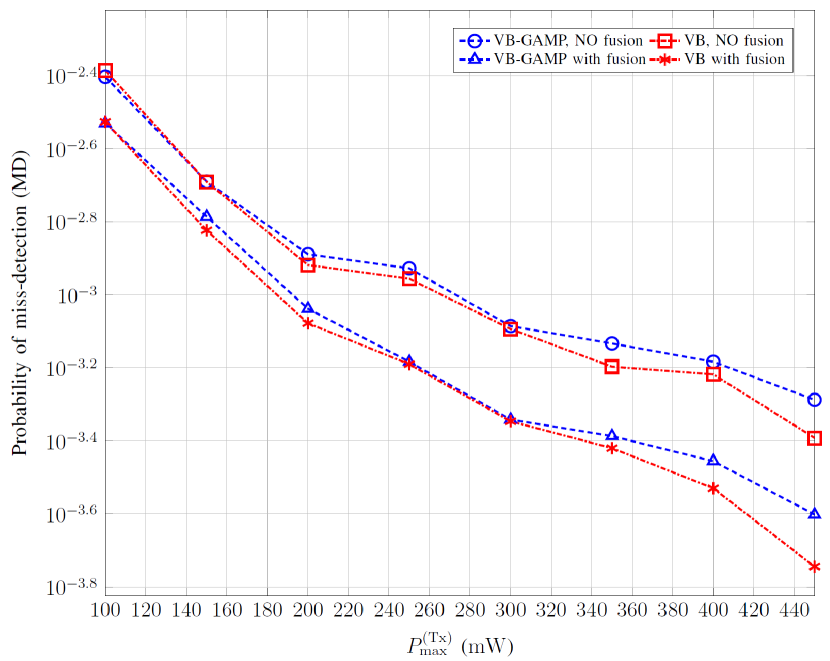
Figure 1: Probability of MD as a function of $P_{\rm max}^{(\rm Tx)}$.

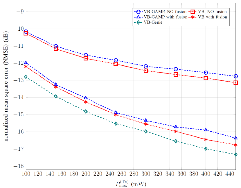
Figure 2: NMSE as a function of $P_{\rm max}^{(\rm Tx)}$.

IV Simulation Results

We numerically evaluate the probability of miss-detection (MD)and the normalized mean square error (NMSE)performances to demonstrate the efficacy of the proposed flexible GFRA framework. We deploy $20$ APs with $2$ antennas each at a height of $10$ m and $200$ UEs uniformly at random in a square area of $1\times 1$ ${\rm km}^{2}$. We set the number of active UEs to $20$. We use a wrap-around technique to approximately generate an infinitely large network with $40$ antennas and $20$ active UEs per ${\rm km}^{2}$ [15, 16]. We sample the pilot lengths from a uniform distribution between $20$ and $24$ ($W=24$). We use complex Gaussian pilots of unit energy and a bandwidth of $1$ MHz. The noise power spectral density is set to $-169$ dBm, and the LSFC (in dB) of the channel between the $k$-th UE and the $\ell$-th AP is generated as: $\beta_{\ell k}=-140.6-36.7\log_{10}\left(d_{\ell k}\right)+\Psi_{\ell k}$, where $d_{\ell k}$ is the distance in km, $\Psi_{\ell k}$ is the log-normal shadowing distributed as $\mathcal{N}(0,\sigma_{\rm sf}^{2})$ and $\sigma_{\rm sf}$ is set to $4$ dB [17]. We set $a$ and $b$ to $10^{-10}$.

We vary $P_{\rm max}^{\rm(Tx)}$ from $100$ mW to $450$ mW in our simulations. We adopt the UE-centric power allocation scheme developed in [18] to set the instantaneous transmit power (denoted $P_{k}^{\rm(Tx)}$) of the $k$-th UE as: $P_{k}^{\rm(Tx)}=P_{\rm max}^{\rm(Tx)}\frac{\min_{k^{\prime}}\beta_{\ell_{k^{\prime}}^{(\rm M)}k^{\prime}}}{\beta_{\ell_{k}^{(\rm M)}k}}$, $k\in\{1,\ldots,K\}$. This scheme makes sure only the UEs with the least LSFC to any AP transmits with the maximum power ensuring fairness among them. We set the maximum number of iterations for all the algorithms to $250$, which means that the Steps $4$ to $15$ in the Algorithm 1 are executed either till convergence or for a maximum of $\left\lfloor\frac{250}{\rm MAX\_ITER}\right\rfloor$ iterations.

Fig. 1 compares the probability of MD of the distributed latent-variable fusion based UE activity detection and the state-of-the-art distributed VB based procedures (with legend entries “NO fusion”: Steps $4$ and $10$ to $15$ in Algorithm 1 are not executed for this). This figure shows that our proposed flexible framework with variable pilot lengths is able to achieve a good UE detection performance irrespective of whether we use a latent variable fusion or not. Moreover, we see that the detection probability improves by a large margin by combining the posterior statistics of the latent variables at the CPU (legend entries “with fusion”). For example, the maximum transmit power of the UEs can be reduced by around $100$ mW to achieve a probability of MD of $0.08\leavevmode\nobreak\ \%$ using the latent variable fusion approach, which leads to large power savings to the UEs. This also shows that the posterior statistics obtained at the master APs are more reliable than that of the other APs, which improves the detection rate.

Fig. 2 depicts the NMSE performances of the distributed VB channel estimation procedures with and without latent variable fusion. We also compare against a genie-aided channel estimator which has a prior knowledge about the active UEs, and therefore can be considered as a lower bound for the NMSE of the developed latent variable fusion based estimators. We clearly see that by utilizing the posterior statistics sent from the APs to the CPU, the performance moves close to the lower bound. For instance, we can achieve the same NMSE of VB-Genie for the developed distributed VB algorithm by expending only a little less than $50$ mW of the maximum transmit power. Moreover, from the Figures 1 and 2, we observe that a VB-GAMP implementation results in a marginal loss in performance compared to VB procedure.

V Conclusions & Future Work

We proposed a novel flexible framework for GFRA in cell-free massive MIMO systems which admitted variable length signature sequences for the UEs. We formulated the joint UE activity detection and the distributed channel estimation as a sparse support and signal recovery problem, and described a Bayesian learning procedure to solve it. To enhance the detection performance, we devised a latent-variable fusion mechanism to combine the posterior statistics inferred at the APs. We also referred to an intricate point to encode the information bits from the active UEs without any additional transmit power. Finally, we numerically evaluated the NMSE and the MD performances of the SBL algorithm to illustrate the efficacy of the generalized framework. We aim to investigate the joint activity detection, channel estimation, and data detection for the flexible framework as part of our future work.

References

- [1] Z. Chen, F. Sohrabi, and W. Yu, “Sparse activity detection for massive connectivity,” IEEE Trans. Signal Process., vol. 66, no. 7, pp. 1890–1904, 2018.
- [2] L. Liu, E. G. Larsson, W. Yu, P. Popovski, C. Stefanovic, and E. de Carvalho, “Sparse signal processing for grant-free massive connectivity: A future paradigm for random access protocols in the internet of things,” IEEE Signal Process. Mag., vol. 35, no. 5, pp. 88–99, 2018.
- [3] K. Senel and E. G. Larsson, “Grant-free massive mtc-enabled massive MIMO: A compressive sensing approach,” IEEE Trans. Commun., vol. 66, no. 12, pp. 6164–6175, 2018.
- [4] L. Liu and W. Yu, “Massive connectivity with massive MIMO—part i: Device activity detection and channel estimation,” IEEE Trans. Signal Process., vol. 66, no. 11, pp. 2933–2946, 2018.
- [5] Y. Li, M. Xia, and Y.-C. Wu, “Activity detection for massive connectivity under frequency offsets via first-order algorithms,” IEEE Trans. Wireless Commun., vol. 18, no. 3, pp. 1988–2002, 2019.
- [6] U. K. Ganesan, E. Björnson, and E. G. Larsson, “Clustering-based activity detection algorithms for grant-free random access in cell-free massive MIMO,” IEEE Trans. Commun., vol. 69, no. 11, pp. 7520–7530, 2021.
- [7] Z. Chen, F. Sohrabi, and W. Yu, “Sparse activity detection in multi-cell massive MIMO exploiting channel large-scale fading,” IEEE Trans. Signal Process., vol. 69, pp. 3768–3781, 2021.
- [8] W. Chen, H. Xiao, L. Sun, and B. Ai, “Joint activity detection and channel estimation in massive MIMO systems with angular domain enhancement,” IEEE Trans. Wireless Commun., vol. 21, no. 5, pp. 2999–3011, 2022.
- [9] Y. Li, Q. Lin, Y.-F. Liu, B. Ai, and Y.-C. Wu, “Asynchronous activity detection for cell-free massive MIMO: From centralized to distributed algorithms,” IEEE Trans. Wireless Commun., vol. 22, no. 4, pp. 2477–2492, 2023.
- [10] H. Zhang, Q. Lin, Y. Li, L. Cheng, and Y.-C. Wu, “Activity detection for massive connectivity in cell-free networks with unknown large-scale fading, channel statistics, noise variance, and activity probability: A bayesian approach,” IEEE Trans. Signal Process., vol. 72, pp. 942–957, 2024.
- [11] M. E. Tipping, “Sparse Bayesian learning and the relevance vector machine,” Journal of machine learning research, vol. 1, no. Jun, pp. 211–244, 2001.
- [12] D. Wipf and B. Rao, “Sparse Bayesian learning for basis selection,” IEEE Trans. Signal Process., vol. 52, no. 8, pp. 2153–2164, 2004.
- [13] C. M. Bishop, Pattern Recognition and Machine Learning. Springer New York, 2006.
- [14] M. Al-Shoukairi, P. Schniter, and B. D. Rao, “A GAMP-based low complexity sparse Bayesian learning algorithm,” IEEE Trans. Signal Process., vol. 66, no. 2, pp. 294–308, 2018.
- [15] T. L. Marzetta, E. G. Larsson, and H. Yang, Fundamentals of massive MIMO. Cambridge University Press, 2016.
- [16] Ö. T. Demir, E. Björnson, L. Sanguinetti et al., “Foundations of user-centric cell-free massive mimo,” Foundations and Trends® in Signal Processing, vol. 14, no. 3-4, pp. 162–472, 2021.
- [17] Further advancements for E-UTRA physical layer aspects (Release 9). 3GPP TS 36.814, Mar. 2010.
- [18] J. Bai and E. G. Larsson, “Activity detection in distributed MIMO: Distributed AMP via likelihood ratio fusion,” IEEE Wireless Comm. Letters, vol. 11, no. 10, pp. 2200–2204, 2022.