Pheromone-Guided Navigation of Potential Mates: A Distinct Exploration Strategy

Abstract\\

Animals, especially insects, navigate their environments using complex strategies that integrate responses to chemical signals such as pheromones. The relative importance an insect places on foraging, finding a mate or other tasks can significantly influence its movement patterns. This study uncovers the distinct exploration strategies that emerge when these priorities vary. A new model is introduced that explicitly treats a pair of insects and their response to each other’s pheromones. The strategy results in dynamics that exhibit characteristic anomalous scaling in displacement and non-Gaussian distributions of position; specifically, compressed exponential distributions for the number of encounters and the total duration of encounters. Our model not only elucidates these emergent behaviours but also provides insight into optimizing encounter frequencies. These strategies can be inverted to design pheromone-based traps for luring target species to specific areas for removal. The model is also applicable more broadly to pairs of agents that both respond to the paths traced by themselves and each other.

I Introduction

Animal exploration strategies often deviate from simple random movement [1, 2]. This complexity arises particularly in species relying on chemical signals (semiochemicals) such as pheromones for communication and navigation [3, 4]. Traditional random walk models have proven valuable for studying such processes, yet increasing evidence reveals the need for more sophisticated approaches to capture the nontrivial dynamics observed in nature [5]. Recent efforts have focused on deviations from classical diffusion processes, compelling the development of models that accommodate these complexities [6, 7].

One such complexity arises in systems exhibiting anomalous diffusion, where the mean squared displacement (MSD) scales nonlinearly with time—a phenomenon ubiquitous in physical, financial, artificial, and biological systems [8, 9, 10, 11, 12, 13, 14, 15]. In biological contexts, this behaviour often stems from memory effects or interactions with evolving environments. Insects, for example, modify their environment by laying down pheromone trails, which subsequently influence not only their own movements but also those of others in their vicinity [16, 17, 18]. This phenomenon extends to living cells that alter their surroundings by depositing biochemical signals or mechanically remodelling the extracellular matrix [19, 20, 21], as well as large animals that mark their territories [22, 23]. These feedback loops, reminiscent of self-organizing systems, lead to emergent behaviours that deviate sharply from classical diffusion models. Non-Markovian random walks, in which movement decisions depend on the walker’s history, provide a framework for understanding these anomalous behaviours [24, 25, 26, 27, 28, 29, 30, 31, 32, 33].

One established approach for modelling such memory-driven dynamics is the true self-avoiding walk (TSAW), introduced by Amit, Parisi, and Peliti [24]. In the TSAW, movement (transition) probabilities, $p$, depend on the visitation history of each site:

$$p\propto e^{-\beta h_{i}},$$ (1)

where $h_{i}$ represents the number of times site $i$ has been visited, and $\beta$ is a constant analogous to inverse temperature, controlling the strength of self-avoidance. The TSAW extends the concept of the self-avoiding walk (SAW) [34, 35] that is well-known for modelling the behaviour of flexible chain polymers. Despite its name, the SAW is more accurately described as a ‘self-terminating’ walk, where revisiting a site terminates the walk. In contrast, the TSAW employs a ‘softer’ self-avoidance, where the walker tries to avoid retracing its steps.

Within the TSAW model, when self-interaction is repulsive ($\beta>0$), the time dependence of the MSD, $R^{2}$, as a function of time exhibits distinct scaling laws in different dimensions, $d$, at large times [24, 36, 37, 30, 33, 38]:

$$R^{2}\sim\begin{cases}t^{4/3}\quad&d=1\\ t(\ln t)^{1/2}\quad&d=2\\ t\quad&d\geq 3.\end{cases}$$ (2)

In contrast, introducing an attractive self-interaction ($\beta<0$) dramatically restricts the walker’s movement. This leads to repetitive oscillations between two sites for any dimension $d$, resulting in a constant MSD at large times [30, 38]:

$$R^{2}\to C,$$

where $C$ is a constant depending on $d$ and $\beta$. Introducing a saturation limit for $h_{i}$ (e.g., $h_{i}=0$ for unvisited site $i$, and $h_{i}=1$ if visited) transforms the self-attractive case, preventing walker trapping. This modified model, known as the self-attracting true random walk (SATW) or one-step reinforced random walk, [39, 30, 29, 40, 41, 42, 38], exhibits a diverging MSD at large times:

$$R^{2}\sim\begin{cases}t\quad&d=1\\ t^{2/3}\quad&d=2\\ t\quad&d=3,|\beta|<|\beta_{c}|\\ t^{1/2}\quad&d=3,|\beta|>|\beta_{c}|\\ \end{cases}$$ (3)

Here, $\beta_{c}$ marks a critical value in three dimensions, signifying the transition to a subdiffusive regime.

Natural environments present intricate scenarios, particularly when multiple interacting individuals are involved [43, 44]. For example, the trade-off between food exploration and mate-seeking plays a significant role in shaping insect movement. Insects rely on multiple semiochemicals, such as trail and sex pheromones, to guide their movements and interactions, resulting in complex, correlated behaviour. Foraging insects avoid revisiting previously explored locations due to diminishing chances of finding food, while the presence of sex pheromones draws them toward areas marked by potential mates. This dynamic interaction between food foraging and mate-seeking leads to a collective mode of exploration, particularly in species that deposit different types of semiochemicals [4, 18].

When these behaviours are coupled, they give rise to novel collective dynamics characterized by emergent scaling relations that define new universality classes. As far as we are aware, the study of such active systems, where food-foraging and mate-seeking are intertwined, remains largely unexplored. This research represents an exciting frontier in understanding collective dynamics.

II Method

II.1 The Model

We consider a $d$-dimensional lattice over which two random walkers, A and B, undergo random walks. If we are modelling the paths of insects, A and B could represent a male and a female. The process starts when the walkers are $D_{0}$ apart. Each walker leaves a single, characteristic unit of ‘debris’ upon stepping on the site $i$. Furthermore, in our model the agents prefer to avoid places they have been before, but are attracted to places that the other agent has been before. Thus, this model can represent a pair of insects that are foraging and seeking each other with the debris being the pheromones from each insect. The amount (height) of pheromones released by the agent $X$ (A or B) at site $i$ up to time $t$ reads:

$$h_{i}^{(X)}(t)=\sum_{\tau=1}^{t}\delta_{x_{\tau}^{(X)},i},\quad h_{i}^{(X)}(0)=0\;\forall i,$$ (4)

where $x_{\tau}^{(X)}$ is the position of the agent $X$ at time $\tau$ and $\delta$ is the Kronecker delta. In the example of the insects, this measures the amount of pheromone left by each of the insects at each site as a function of time (see Fig. 1a). Each agent engages with its own debris and that of the other agent differently. The crucial aspect of our model is the transition probability for the agent $X$ moving from the site $i$ to $j$, which is expressed as follows:

$$\begin{split}p^{(X)}_{i\to j}&=\frac{e^{-\beta h_{j}^{(X)}}e^{+\beta^{\prime}h_{j}^{(X^{\prime})}}}{Z}\qquad\beta,\beta^{\prime}\geq 0,\\ Z&\equiv\sum_{j\in\text{nn}_{i}}e^{-\beta h_{j}^{(X)}}e^{+\beta^{\prime}h_{j}^{(X^{\prime})}}\end{split}$$ (5)

where a prime, $X^{\prime}$, indicates the other agent, and $\text{nn}_{i}$ denotes the nearest neighbors of site $i$. The coefficients $\beta\geq 0$ and $\beta^{\prime}\geq 0$ serve as the avoiding and attracting factors, respectively. Note that this model does not allow the agents to stay at the same site at consecutive times, but the agents could move together to a neighbouring site. According to the equation above, at each time step, an agent is more likely to move to sites containing a greater amount of the other agent’s debris and less likely to move to sites with a greater amount of its own. Our model assumes reciprocal behaviour: the agents operate under the same transition rules. These rules incorporate memory effects, as the transition probabilities depend on the values of $h_{i}$, which are themselves determined by the agents’ past locations.

We are interested in calculating the mean-squared distance between two agents, A and B:

$$d^{2}_{t}\equiv\left\langle(x^{(A)}_{t}-x^{(B)}_{t})^{2}\right\rangle,$$ (6)

and the mean end-to-end distance of the path of a single agent, equivalent to MSD for each agent:

$$R^{2}_{t}\equiv\left\langle\left(x_{t}-x_{0}\right)^{2}\right\rangle,$$ (7)

where $\langle\cdot\rangle$ denotes the ensemble average. Since the model assumes reciprocal behaviour, the average MSD will be the same for both agents.

The scaling ansatz held for many anomalous diffusion processes is given by [10, 6, 8]:

$$R^{2}_{t\to\infty}\sim t^{\alpha}(\ln t)^{\hat{\alpha}},$$ (8)

where $\alpha=1$ and $\hat{\alpha}=0$ for normal diffusion, i.e., for non-correlated standard random walks. Superdiffusion refers to the case $\alpha>1$ or $\alpha=1,\hat{\alpha}>0$, while subdiffusion corresponds to $\alpha<1$. Additionally, the increment statistics display a similar behaviour to MSD at large times, offering another measure, called mean-squared increment (MSI) [38]:

$$\Delta^{2}_{t,T}\equiv\left\langle\left(x_{T+t}-x_{T}\right)^{2}\right\rangle$$ (9)

We track two important measures to analyze the evolving interactions between the agents: the frequency of encounters ($m$) and the total time ($\mathcal{T}$) spent in the same place (lattice cell) as they change over time $t$. In the case of non-correlated normal random walks moving in one dimension, the probability distributions of these metrics, $P(m,t)$ and $P(\mathcal{T},t)$, exhibit Gaussian behaviour. However, in two dimensions, these distributions are exponential. Moreover, the probability distribution of each agent’s position, $P(x,t)$, is known to be Gaussian regardless of the dimensionality [14]. Calculating the statistical measures for uncorrelated normal random walks is not the primary focus of this work. Therefore, further details are provided in the Supplementary Material.

The key difference between our model and previous ones lies in the source of attraction within Eq. 5. In our model, the attraction stems from the path laid down by the other walker (agent), not the walker’s own path. This novel interaction gives rise to distinct universality classes and unique behaviours. Furthermore, it provides a model for physical systems such as the pathways of insects driven by different pheromone, and could apply to a broad range of systems including active biological cells and growth of neural networks [45].

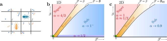
Figure 1: Pheromonal random walks and phase diagrams. (a) Two insects (agents), A and B, represented in orange and blue respectively, collaborate to navigate in a stochastic and correlated manner, moving right, left, up, or down in two dimensions. As they visit sites, each insect deposits a unit of pheromone, indicated by orange circles for insect A and blue circles for insect B. In this configuration, the amount of the orange pheromone at the labelled site $i$ is $h_{i}^{(A)}=1$, while for the blue pheromone is $h_{i}^{(B)}=3$ and at $j$ it is $h_{j}^{(A)}=2,h_{j}^{(B)}=1$. The model assumes that each agent is more likely to move to sites with a greater amount of pheromone of the other agent and less of its own pheromone. (b) The phase diagram for a one-dimensional system. We expect the scaling relation for MSD $R^{2}_{t}\sim t^{\alpha}$ at large times. When $\beta^{\prime}\leq\beta$ (red region), the system manifests superdiffusion with $\alpha=4/3$. The dashed line represents the function $\beta^{\prime}=\mathcal{B}(\beta)$, which separates the orange and blue regions and its exact form is unknown. For $\beta^{\prime}>\mathcal{B}$ (blue region), the system exhibits subdiffusion with an exponent $\alpha$ approaching 1 from below ($\alpha\to 1^{-}$). When $\beta=0$ and $\beta^{\prime}$ is large (purple region), the system exhibits subdiffusion with $\alpha=1/2$. The case where $\beta=\beta^{\prime}=0$ corresponds to normal diffusion (the tiny green region). (c) The phase diagram for a two-dimensional system. The MSD follows the relation $R^{2}_{t}\sim t^{\alpha}(\ln t)^{\hat{\alpha}}$ at large times. Here, for $\beta\leq\beta^{\prime}$ (red region), $\alpha=1$ and $\hat{\alpha}=1/2$. For $\beta^{\prime}>\mathcal{B}_{\text{2D}}$ (blue region), $\alpha\to 0.9$ and $\hat{\alpha}=0$. Unlike the 1D case, we do not observe a unique behaviour for $\beta=0$. The orange regions, $\beta<\beta^{\prime}<\mathcal{B}$, in (b) and (c) are transient regions where the system may not show stable behaviour.

II.2 Computational Details

All data was obtained from random walk simulations with transition probabilities given by eqn. 5 in 1D and 2D and were carried out using code developed in our group. We considered initial separations of $D_{0}=100$ for 1D and $D_{0}=10$ for 2D, with the self-avoidance coefficient set to $\beta=0,0.5$ or $1$ and various values of the attraction coefficient, $\beta^{\prime}$. The ensemble averages were computed over 5 million samples for each parameter set, with some cases requiring over 10 million samples when $\beta^{\prime}>\mathcal{B}$. During the simulation, measures such as the end-to-end distance, increment for each agent and the distance between the two agents were calculated at logarithmically spaced time intervals. Histograms of distances, positions, and encounter metrics were generated at specific time points. Output files were saved and stored for subsequent analysis to determine MSD, mean-squared distance, MSI, position distributions, encounter frequencies, total encounter durations, and their scaling behaviors.

III Results

Due to the reciprocal nature of our model, statistical measures such as $R^{2}_{t}$, and $P(x,t)$ are identical for both agents. Therefore, we report these measures only for the first walker.

The phase diagrams for the diffusion exponents in 1D and 2D (related to Eq. (8)) are shown in Fig. 1. In one dimension, we identify three distinct universality classes: (i) For $\beta^{\prime}\leq\beta$, the diffusion exponent is $\alpha=4/3$, characterizing a superdiffusion regime. (ii) For $\beta^{\prime}>\mathcal{B}$ (where $\mathcal{B}$ depends on $\beta$), the diffusion exponent approaches $\alpha=1$ from below ($\alpha\to 1^{-}$), indicating a pseudonormal (or subdiffusion) regime. This behaviour deviates from normal diffusion, where $\alpha=1$. We will demonstrate that the position probability distribution in this subdiffusion regime is non-Gaussian. The intermediate region ($\beta<\beta^{\prime}<\mathcal{B}$) exhibits a transition between the two regimes. Investigating this region poses practical challenges, as it may require extremely long simulations, and we skip it in this manuscript. (iii) When $\beta=0$, and $\beta^{\prime}$ is large, the system represents subdiffusion with $\alpha=1/2$. Importantly, all these results are independent of the initial distance between the two walkers, $D_{0}$.

Figure 2a demonstrates the time dependence of an agent’s MSD for various values of $\beta^{\prime}$, with a fixed coefficient $\beta=1$ and $D_{0}=100$. Figure 2b displays the mean-squared distance between two agents over time, again with varying $\beta^{\prime}$ values. These curves exhibit similar asymptotic trends compared to $R^{2}_{t}$. The case of $\beta=0$ is unique, as shown in Fig. 2c: for large values of $\beta^{\prime}$, the exponent $\alpha=1/2$. Figure 2d illustrates how the exponent $\alpha$ depends on $\beta^{\prime}$ for three values of $\beta$ (0, 0.5, and 1).

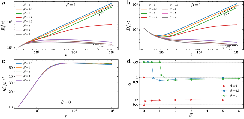
Figure 2: Mean-squared displacement and distance for a 1D model system. Here we plot the statistical measures for the first agent. Due to the reciprocal interaction scheme, the statistics for both agents are identical. (a) $R^{2}_{t}/t$ versus time $t$ is plotted for various $\beta^{\prime}$ with fixed $\beta=1$. Superdiffusion ($\alpha=4/3$; $R_{t}^{2}/t\sim t^{1/3}$ for large $t$) is evident for $\beta^{\prime}\leq 1$, while subdiffusion ($\alpha\to 1^{-};R_{t}^{2}/t\sim t^{0^{-}}$ for large $t$) occurs for $\beta^{\prime}\geq 2$. (b) The mean-squared distance between two agents, $d_{t}^{2}$ is depicted, demonstrating a similar asymptotic behaviour to the mean-squared displacement of each agent. (c) $R^{2}_{t}/t^{1/2}$ is plotted versus $t$ for $\beta=0$ and $\beta^{\prime}>0$, showing that for large values of $\beta^{\prime}$, $\alpha=1/2$ ($R^{2}_{t}/t^{1/2}\to const$) at large $t$. (d) The dependence of $\alpha$ versus $\beta^{\prime}$ is plotted for various values of $\beta=0,0.5$, and $1$. The error bars are smaller than symbol sizes.

The distinct universality classes governing the system’s dynamics are reflected in the behaviour of the position probability distribution, $P(x,t)$, and the encounter-related probability distributions, $P(m,t)$ and $P(\mathcal{T},t)$. These distributions themselves display unique universality classes. Fig. 3a shows the normalized probability distribution function of the first agent for cases $\beta^{\prime}=0,0.5$ and $1$ with fixed $\beta=1$. These distribution functions corresponding to $\beta^{\prime}\leq\beta$ all are symmetric. In the absence of attraction of agents ($\beta^{\prime}=0$), the probability distribution $P(x,t)$ exhibits two peaks. As $\beta^{\prime}$ increases, these peaks shift towards the origin, ultimately overlapping when $\beta^{\prime}=1$. To demonstrate the evolution of $P(x,t)$, we calculated the probability distributions at $t=5\times 10^{5},10^{6},5\times 10^{6}$, and $10^{7}$. Fig. 3b illustrates this for the case of $\beta^{\prime}=0$. As shown in the inset, rescaling $x\to x/t^{2/3}$ and $P\to t^{2/3}P$ leads to a collapse of the curves onto a single curve. This curve exhibits a thin tail (faster-than-Gaussian decay) that follows the relation $\exp(-az^{3.3})$, with $a$ dependent on $\beta$ and $\beta^{\prime}$. The thin-tailed behaviour is also observed for all $\beta^{\prime}\leq\beta$, as exemplified by the case of $\beta^{\prime}=1$ in the inset of Fig. 3c where the tail follows the $\exp(-az^{3})$.

When $\beta^{\prime}>\mathcal{B}$, the distribution functions $P(x,t)$ lose their symmetry, where $\mathcal{B}\approx 1.5$ for fixed $\beta=1$. If we set the initial distance between two agents to $D_{0}=0$, one could expect a symmetric function for $P(x,t)$. The asymmetric behaviour is evident in Fig. 3d for $\beta^{\prime}=1.5,5$, and $6$ with fixed $\beta=1$. For all $\beta^{\prime}>\mathcal{B}$, the appropriate transformation to collapse the $P(x,t)$ curves for different times is $x\to(x-\frac{D_{0}}{2})/t^{2/3}$ and $P\to tP$. The inset of Fig. 3e demonstrates this collapse for the case $\beta^{\prime}=5$.

The position probability distribution functions for cases with $\beta=0$ and $\beta^{\prime}>\mathcal{B}\approx 0.5$ exhibit strikingly different behaviour. As shown in Fig. 3f, for $\beta=0$ and $\beta^{\prime}=5$, the first agent (initially at the origin) remains largely confined within a region $x\lessapprox 100$. Note that within the region $x\lessapprox-35$, rescaling $x\to t^{-1/2}x$ and $P\to tP$ collapses the distribution curves for different times $t$ onto a single curve.

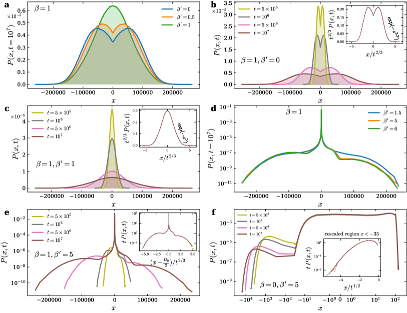
Figure 3: Position probability distribution function. (a) The $P(x,t)$ of the first agent for $\beta^{\prime}=0,0.5$, and $1$ (fixed $\beta=1$) at time $t=10^{7}$. Distributions for $\beta^{\prime}\leq\beta$ are symmetric. With increasing $\beta^{\prime}$, the bimodal peaks of $P(x,t)$ shift towards the origin, overlapping at $\beta^{\prime}=1$. (b) and (c) Time evolution of the probability distribution function for $\beta^{\prime}=0$ and $\beta^{\prime}=1$, respectively. Inset demonstrates that rescaling $x\to t^{-2/3}x$ and $P\to t^{2/3}P$ collapses the curves for different times onto a single curve. The tail of the collapsed curve follows $\exp(-z^{3.3})$ for $\beta^{\prime}=0$ and $\exp(-z^{3})$ for $\beta^{\prime}=1$, where $z\equiv x/t^{2/3}$. (d) For $\beta^{\prime}\geq\mathcal{B}$, where $\mathcal{B}\approx 1.5$ for $\beta=1$, the probability distributions $P(x,t)$ are asymmetric. (e) For $\beta=1,\beta^{\prime}=5$ (actually for all $\beta^{\prime}\geq\mathcal{B}$), rescaling $x\to t^{-2/3}(x-D_{0}/2)$ and $P\to tP$ collapses the $P(x,t)$ curves for different times. Inset demonstrates this collapse. (f) Position probability distribution for $\beta=0$, $\beta^{\prime}=5$. The first agent is largely confined within a region less than about $100$ and explores primarily $x<0$. Inset: For $x\lessapprox-35$, rescaling $x\to t^{-1/2}x$ and $P\to tP$ collapses the curves. Note that the initial distance between two agents for all simulations is $D_{0}=100$.

The distribution of the number of encounters between the agents ($m$) up to time $t$ is a crucial metric. For insects that are foraging and seeking a mate, this would be the distribution of the frequency of the insects meeting. Figure 4(a) shows the probability distributions $P(m,t=10^{7})$ for $\beta^{\prime}=0,0.5$, and $1$ in a semi-log plot. The inset highlights their compressed exponential behaviour: $\exp(-az^{4/3})$, where $a$ depends on $\beta$ and $\beta^{\prime}$. Figure 4b shows time-dependent distributions for $\beta=1,\beta^{\prime}=1$. The inset demonstrates that by rescaling $m\to t^{-1/3}m$ and $P\to t^{1/3}P$, curves for different times collapse onto a single curve. This transformation holds for all $\beta^{\prime}\leq\beta$. Figure 4c depicts the distribution functions for $\beta^{\prime}=1.5,3$, and $5$ (semi-log plot), revealing exponential decay: $\exp(-am)$. The inset confirms that these probability distributions are time-independent, so $P(m,t)\sim\exp(-am)$, with $a$ depending on $\beta$ and $\beta^{\prime}$. Figure 4d, for the case with self-interaction off ($\beta=0,\beta^{\prime}>0$), exhibits a similar exponential behaviour in $P(m,t)$ as seen in Fig. 4c. Thus, the fundamental behaviour of the exploration changes from superdiffusive to subdiffusive with the strength of the attract of the insects to each other’s paths.

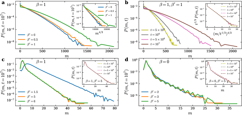
Figure 4: Probability distribution of encounters. (a) Probability distribution $P(m,t=10^{7})$ of encounters for $\beta^{\prime}=0,0.5$, and $1$ with fixed $\beta=1$ over the period $t=10^{7}$. The inset shows the distributions follow a compressed exponential function, $\exp(-az^{4/3})$, where $a=a(\beta,\beta^{\prime})$. (b) Time-dependent probability distributions of encounters for $\beta=1,\beta^{\prime}=1$. The inset demonstrates the collapse of curves onto a single curve using the transformation $m\to t^{-1/3}m$ and $P\to t^{1/3}P$. This scaling holds for all $\beta^{\prime}\leq\beta$. (c) $P(m,t=10^{7})$ for $\beta^{\prime}=1.5,5$, and $6$ with fixed $\beta=1$ in a semi-log plot. The distributions display exponential decay, $\exp(-am)$. The inset confirms that the distributions are time-independent. (d) $P(m,t=10^{7})$ for case $\beta=0,\beta^{\prime}=2,3,5$. Similar to (c), an exponential decay behaviour is observed, but not very strictly.

Another crucial metric is the probability distribution of the duration of meetings up to time $t$, denoted as $P(\mathcal{T},t)$. Fig. 5a shows the probability distribution at $t=10^{7}$ for $\beta^{\prime}=0,0.5$, and 1 in a semi-log plot. The inset demonstrates that $P(\mathcal{T},t)$ follows a compressed exponential function, $\exp(-az^{4/3})$, similar to the behaviour observed for $P(m,t)$ in Fig. 4a. Figure 5b illustrates the time evolution of $P(\mathcal{T},t)$ at various times ($t=5\times 10^{5},10^{6},5\times 10^{6}$, and $10^{7}$). The inset shows that by rescaling $\mathcal{T}\to\mathcal{T}/t^{1/3}$ and $P\to t^{1/3}P$, these curves collapse onto a single curve. For $\beta^{\prime}$ exceeding the transition value $\mathcal{B}$, the probability distributions exhibit markedly different behaviour. As shown in Fig. 5c, the probability distribution function has high values for finite $\mathcal{T}$, indicating that agents spend limited time together despite a higher attraction coefficient. The three curves, corresponding to $\beta^{\prime}=1.5,5$, and 6, exhibit a compressed exponential behaviour, $\exp(a_{1}z^{1.5})$, in the region $0.1\lesssim\mathcal{T}/t\lesssim 0.6$, and $\exp(a_{2}z^{5})$ for $0.6\lesssim\mathcal{T}/t\lesssim 0.9$. The coefficients $a_{1}$ and $a_{2}$ depend on $\beta$ and $\beta^{\prime}$. Fig. 5d depicts the time-dependence of $P(\mathcal{T},t)$ for $\beta=1,\beta^{\prime}=5$. The inset reveals that rescaling $\mathcal{T}\to\mathcal{T}/t$ and $P\to t^{1.4}P$ leads to a collapse of the curves.

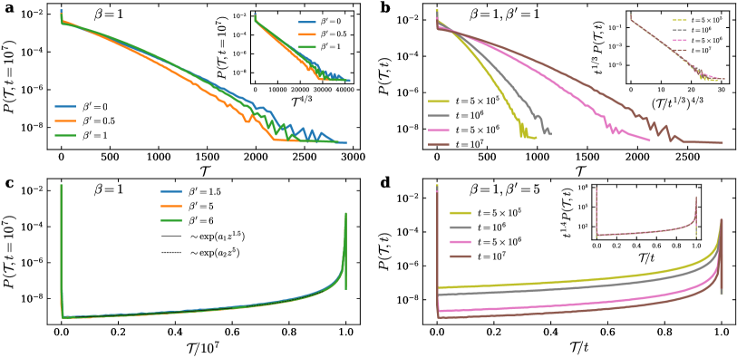
Figure 5: Probability distribution of meeting duration. (a) Probability distribution $P(\mathcal{T},t=10^{7})$ of the total duration of meetings for $\beta^{\prime}=0,0.5$, and $1$ with fixed $\beta=1$. The inset shows the distributions follow a compressed exponential, $\exp(-az^{4/3})$, where the coefficient $a=a(\beta,\beta^{\prime})$. (b) Time-dependent probability distributions for $\beta=1,\beta^{\prime}=1$. The inset demonstrates that rescaling $\mathcal{T}\to\mathcal{T}/t^{1/3}$ and $P\to t^{1/3}P$ collapses the curves for different times onto a single curve. (c) $P(\mathcal{T},t)$ for superdiffusion region with $\beta^{\prime}=1.5,5$, and 6. Distributions exhibit high values for small $\mathcal{T}$, indicating limited duration of meetings. Two compressed exponential regimes are observed: $\exp(a_{1}z^{1.5})$ for $0.1\lesssim\mathcal{T}/t\lesssim 0.6$ (black solid line) and $\exp(a_{2}z^{5})$ for $0.6\lesssim\mathcal{T}/t\lesssim 0.9$ (black dashed line). The coefficients $a_{1}$ and $a_{2}$ are functions of $\beta$ and $\beta^{\prime}$. (d) $P(\mathcal{T},t=10^{7})$ for $\beta=1,\beta^{\prime}=5$. The inset shows that the curves for different times collapse under the rescaling $\mathcal{T}\to\mathcal{T}/t$ and $P\to t^{1.4}P$.

In two dimensions, the system exhibits markedly different behaviour (see Fig. 1b). We initialize the simulation with the first agent (A) at the origin ($x=y=0$) and the second agent (B) at position ($x=D_{0},y=0$). The asymptotic behaviours do not relate to the value of $D_{0}$, at least for moderate values of $D_{0}$. Here, we set $D_{0}=10$. For $\beta^{\prime}\leq\beta$, superdiffusion is observed with $\alpha=1$ and $\hat{\alpha}=1/2$. While Fig. 6a suggests a slight deviation from this behaviour for $\beta=1$ and $\beta^{\prime}=1$, we turn to the mean-squared increment (Eq. 9) to obtain more reliable statistics. As shown in Fig. 6b, the curves for different values of $T$ ultimately reach a plateau for large $t$, confirming the superdiffusive regime. When $\beta^{\prime}\geq\mathcal{B}$, the system transitions to a subdiffusion regime with $\alpha\to 0.9$ and $\hat{\alpha}=0$, as illustrated in Figs. 6c-d. In our case, $\mathcal{B}\approx 2$ when $\beta=1$.

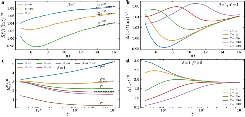
Figure 6: Mean-squared displacement for a 2D model system. (a) MSD divided by $t(\ln t)^{1/2}$ versus $\ln t$ for $\beta^{\prime}=0,0.5,1$ with fixed $\beta=1$. While a slight deviation from the expected $\alpha=1,\hat{\alpha}=1/2$ behaviour is observed for $\beta=1,\beta^{\prime}=1$, further analysis is needed for confirmation. (b) Mean-squared increment for various $T$ values, demonstrating a plateau at large $T$ and $t$ for $\beta=1,\beta^{\prime}=1$. (c) MSD for various $\beta^{\prime}=2,3,4,5$, and $6$ with fixed $\beta=1$. The brown curve represents the case $\beta=0,\beta^{\prime}=5$. The asymptotic behaviour indicates a transition to a subdiffusion regime for $\beta^{\prime}>\mathcal{B}$, with $\alpha=0.9$ and $\hat{\alpha}=0$. (d) $\Delta^{2}_{t,T}/t^{0.9}$ versus time is plotted for various $T$ (fixed $\beta=1,\beta^{\prime}=5$). The curves reaching a plateau confirm the exponents, $\alpha=0.9$ and $\hat{\alpha}=0$.

We analyze the position probability distribution of the first agent for various $\beta^{\prime}$ with fixed $\beta=1$ (Fig. 7). For $\beta^{\prime}\leq\beta$, the distributions exhibit thin tails. However, when $\beta^{\prime}>\mathcal{B}$, the distributions transition to a fat-tailed (slower-than-Gaussian decay) behaviour.

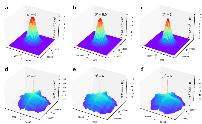
Figure 7: Position probability distribution function for a 2D model system. (a)-(f) Position probability distributions at $t=10^{7}$ for $\beta^{\prime}=0,0.5,1,3,4,5$, with fixed $\beta=1$. (a)-(c) exhibit thin-tailed distributions while (d)-(f) show fat-tailed ones.

IV Discussion

The results of our 1D model reveal significant deviations from classical diffusion, driven by the trade-off between self-avoidance and attraction between agents. These dynamics manifest in distinct scaling behaviours, highlighting the complex interactions that arise from pheromone-guided exploration strategies. Table 1 summarizes the key findings from our 1D model. The observed time-dependent probability distributions follow the scaling form:

$$P(u,t)\sim t^{-\zeta_{u}}f_{u}(u/t^{\nu_{u}}),$$ (10)

where $u$ represents variables such as position ($x$ or $x-D_{0}$), number of encounters ($m$), and total duration of encounters ($\mathcal{T}$). The exponents $\zeta_{u}$ and $\nu_{u}$ characterize the scaling behaviour, and $f_{u}$ represents a universal scaling function. In thin-tailed distributions, the exponents $\zeta_{u}$ and $\nu_{u}$ are equal due to the normalizability of the probability distributions. However, in fat-tailed distributions, these exponents may not be equal [46, 47].

The mean distance between two agents exhibits asymptotic behaviour similar to MSD for all values of $\beta$ and $\beta^{\prime}$ in any dimension (see Fig. 2b and Supplementary Figures S2 and S5). In a simplified scenario with independent walkers, we can envision the first agent as stationary at the origin while the second agent takes two steps at each time increment. This leads to a scaling equivalence: the distance between the second agent and the origin at time $t$ is analogous to the single-walker’s MSD at time $2t$, $R^{2}_{2t}$. When walkers’ trajectories are correlated to each other’s traces, a mean-field approach could be applicable. A crucial assumption for this approach is a uniform debris profile across the lattice. If we also maintain the reciprocal transition probability scheme, the simple interpretation of shifted origins for calculating the distance still remains valid.

For a purely self-interacting walker ($\beta>0,\beta^{\prime}=0$), our model reduces to the well-studied true self-avoiding walk (TSAW) model [24, 30, 38]. For all values of $\beta^{\prime}\leq\beta$, we observe thin-tailed position distributions with $\zeta_{x}=\nu_{x}=2/3$, but different shapes. Interestingly, increasing $\beta^{\prime}$ from zero to $\beta$ transforms the distribution from a symmetric two-peaked form to a symmetric single-peak function (Fig. 3a). Furthermore, the exponent $\alpha=4/3$, characteristic of the TSAW, emerges for all $\beta^{\prime}\leq\beta$ (Fig. 2d). A mean-field approach could provide insights into this behaviour: at large times, if we assume $h^{(A)}_{i}\approx h^{(B)}_{i}\approx\bar{h}$, the transition probability in Eq. (5) becomes proportional to $\exp[-(\beta-\beta^{\prime})\bar{h}]$. Since $\beta\geq\beta^{\prime}$, this effectively maps our model to the TSAW regime. However, for $\beta^{\prime}>\mathcal{B}$, this interpretation may not hold due to strong non-ergodicity and the significant influence of extreme events in the probability distributions of position and inter-agent distance.

A particularly intriguing aspect lies in the likelihood of meeting. Although Supplementary Fig. S6 suggests Gaussian distributions for $m$ and $\mathcal{T}$ in non-correlated normal RWs, our model reveals compressed exponential functions for both $P(m,t)$ and $P(\mathcal{T},t)$, as shown in Figs. 4a-b, 5a-b. For $P(m,t)$ this slower decay compared to Gaussian distributions implies a higher frequency of observing a large number of meetings, and for $P(\mathcal{T},t)$ it implies a higher frequency of long total meeting durations within excursions. This is observed even though our walkers exhibit a greater increase in MSD with time than in non-correlated random walks. Thus, by tuning the values of $\beta$ and $\beta^{\prime}$, we can optimize the distribution of the meetings. In this regime, $\zeta_{m}=\nu_{m}=1/3$ and $\zeta_{\mathcal{T}}=\nu_{\mathcal{T}}=1/3$.

Strong attraction to another agent though preferred movement to lattice points with their debris leads to the emergence of fundamentally distinct dynamics within the system. For inter-attraction coefficients $\beta^{\prime}$ exceeding both $\beta$ and a specific threshold $\mathcal{B}$, the exponent $\alpha$ asymptotically approaches $1^{-}$ (as seen in Fig. 2a). While the near-unity exponent might suggest ‘normal’ diffusion, the fat-tailed position probability distribution (Fig. 3) reveals a significant departure from true Gaussian behaviour. The term ‘pseudonormal’ could aptly describe this regime. Moreover, the meeting probabilities in this regime show non-Gaussian distributions. The probability $P(m,t)$ reaches a steady value (time-independent) for large times and also decays exponentially. The function $P(\mathcal{T},t)$ displays complex time-dependence (Figs. 5c-d). While $P(\mathcal{T},t)$ peaks near $\mathcal{T}\approx 0$, it also has a significant probability around $\mathcal{T}\approx t$. This indicates that while walkers typically have short encounters, there remains a possibility of longer durations. The scaling exponents in this regime are $\zeta_{x}=1,\nu_{x}=2/3$, $\zeta_{m}=\nu_{m}=0$ and $\zeta_{\mathcal{T}}=1.4,\nu_{\mathcal{T}}=1$.

A particularly intriguing scenario emerges when self-repulsion is absent, while strong inter-attraction exists between agents ($\beta^{\prime}>\mathcal{B},\beta=0$). In this regime, agents can become temporarily localized within regions, leading to subdiffusion with $\alpha=1/2$. Interestingly, this exponent matches the three-dimensional true self-avoiding walk (Eq. 3). The fat-tailed asymmetric $P(x,t)$ for the first agent (Fig. 3f) reflects the initial separation distance $D_{0}$ and a typical preference for movement to the left (first agent) and right (second agent).

This regime exhibits strong non-ergodicity, necessitating extensive sampling for ensemble averaging. It contrasts sharply with the $\beta>0,\beta^{\prime}>\mathcal{B}$ case, even though both fall into the broader subdiffusion category. We do not observe this contrasting behaviour in 2D or higher dimensions, likely due to the increased freedom of movement compared to the constraints imposed by the 1D open boundary conditions. The scaling exponents for $P(x,t)$ are $\zeta_{x}=1,\nu_{x}=1/2$, but the scaling exponents for measures of encounter frequency and duration align with the pseudonormal regime ($\beta>0,\beta^{\prime}>\mathcal{B}$).

Table 1: The asymptotic behaviour of various measures for 1D model systems. All coefficients $a,a_{1}$ and $a_{2}$ for each measure are independent and may depend on the values $\beta$ and $\beta^{\prime}$. $D_{0}$ is the initial ($t=0$) distance between two agents. $\mathcal{B}$ is a function of $\beta$.

	$0\leq\beta^{\prime}\leq\beta$	$\beta^{\prime}>\mathcal{B},\beta>0$	$\beta^{\prime}>\mathcal{B},\beta=0$	$\beta^{\prime}=\beta=0$
$R^{2}_{t\to\infty}$	$t^{4/3}$	$t^{1^{-}}$	$t^{1/2}$	$t$
$d^{2}_{t\to\infty}$	$R^{2}_{t\to\infty}$	$R^{2}_{t\to\infty}$	$R^{2}_{t\to\infty}$	$R^{2}_{t\to\infty}$
$P(x,t)$	$t^{-2/3}f\left(\dfrac{x}{t^{2/3}}\right)$, $f$ is thin-tailed	$t^{-1}f\left(\dfrac{x-D_{0}/2}{t^{2/3}}\right)$ $f$ is fat-tailed	$t^{-1}f\left(\dfrac{x}{t^{1/2}}\right)$ for $x\ll 0$ $f$ is fat-tailed	$t^{-1/2}f\left(\dfrac{x}{t^{1/2}}\right)$, $f(z)=e^{-az^{2}}$
$P(m,t)$	$t^{-1/3}f\left(\dfrac{m}{t^{1/3}}\right)$ $f(z)=e^{-az^{4/3}}$	$e^{-am}$	not conclusive, but should be similar to $\beta^{\prime}>\mathcal{B}$, $\beta>0$	$t^{-1/2}f\left(\dfrac{m}{t^{1/2}}\right)$, $f(z)=e^{-az^{2}}$
$P(\mathcal{T},t)$	$t^{-1/3}f\left(\dfrac{\mathcal{T}}{t^{1/3}}\right)$, $f(z)=e^{-az^{4/3}}$	$t^{-1.4}f\left(\dfrac{\mathcal{T}}{t}\right)$ $f(z)=e^{a_{1}z^{1.5}}$, $0.1\lesssim z\lesssim 0.6$ $f(z)=e^{a_{2}z^{5}}$, $0.6\lesssim z\lesssim 0.9$	not conclusive, but should be similar to $\beta^{\prime}>\mathcal{B}$, $\beta>0$	$t^{-1/2}f\left(\dfrac{\mathcal{T}}{t^{1/2}}\right)$, $f(z)=e^{-az^{2}}$

Our simulations in two dimensions reveal two distinct regimes: superdiffusion and subdiffusion (Fig. 6, Table 2). When $\beta^{\prime}\leq\beta$, we observe scaling exponents ($\alpha=1,\hat{\alpha}=1/2$) consistent with the true self-avoiding walk (TSAW). The probability distribution $P(x,y,t)$ exhibits symmetry and thin tails, further emphasized by $P(x,y=0,t)$ and $P(x=0,y,t)$ (Supplementary Fig. S10). Interestingly, two-dimensional scaling exponents deviate from the relation in Eq. 10, instead including logarithmic terms in the position and distribution functions for the encounter frequency:

$$P(u,t)\sim t^{-\zeta_{u}}(\ln t)^{-\hat{\zeta}_{u}}\,f_{u}\left(\frac{u}{t^{{\nu}_{u}}(\ln t)^{\hat{\nu}_{u}}}\right),$$ (11)

where $\zeta_{x}=1$, $\hat{\zeta}_{x}=1/2$, $\nu_{x}=1/2$, $\hat{\nu}_{x}=1/4$, $\zeta_{m}=0$, $\hat{\zeta}_{m}=1/2$, $\nu_{m}=0$, and $\hat{\nu}_{m}=1/2$. The exponents for $\mathcal{T}$ are the same as those for $m$.

For $\beta^{\prime}>\mathcal{B}_{\text{2D}}$, the system transitions to a unique subdiffusive universality class with $\alpha=0.9$ and $\hat{\alpha}=0$. These exponents stand out in the context of subdiffusion. The position distribution scaling exponents are $\zeta_{x}=1$ and $\nu_{x}=0.9/2$. These findings highlight the distinctive behaviours that emerge in two dimensions when there is a strong attraction to the other agent’s debris.

Table 2: The asymptotic behaviour of various measures for 2D model systems. All coefficients $a$ for each measure are independent and may depend on the values $\beta$ and $\beta^{\prime}$. $D_{0}$ is the initial ($t=0$) distance between two agents. $\mathcal{B}_{\text{2D}}$ is a function of $\beta$.

	$0\leq\beta^{\prime}\leq\beta$	$\beta^{\prime}>\mathcal{B}_{\text{2D}}$	$\beta^{\prime}=\beta=0$
$R^{2}_{t\to\infty}$	$t(\ln t)^{1/2}$	$t^{0.9}$	$t$
$d^{2}_{t\to\infty}$	$R^{2}_{t\to\infty}$	$R^{2}_{t\to\infty}$	$R^{2}_{t\to\infty}$
$P(\vec{x},t)$	$t^{-1}(\ln t)^{-1/2}f\left(\dfrac{\vec{x}}{t^{1/2}(\ln t)^{1/4}}\right)$	$t^{-1}f\left(\dfrac{\vec{x}-\vec{D}_{0}}{t^{0.9/2}}\right)$	$t^{-1}f\left(\dfrac{\vec{x}}{t^{1/2}}\right)$ $f(z)=e^{-az^{2}}$
$P(m,t)$	$(\ln t)^{-1/2}f\left(\dfrac{m}{(\ln t)^{1/2}}\right)$, $f(z)=e^{-az}$	not conclusive	$(\ln t)^{-1}f\left(\dfrac{m}{\ln t}\right)$ $f(z)=e^{-az}$

V Conclusion

Our study introduces a model for a class of systems with two distinct agents that avoid retracing their own paths but seek the other agent. This dynamic demonstrates a distinctive exploration strategy that is shaped by the interplay between foraging and mating of insects guided by the deposition of pheromones. Our findings reveal distinct phases — superdiffusion and subdiffusion — determined by the balance between self-avoiding ($\beta$) their own path and attraction ($\beta^{\prime}$) to the other agent’s path. In the case of insect behaviour, this work highlights how prioritising seeking a mate over foraging (small $\beta$ and large $\beta^{\prime}$) can fundamentally alter movement patterns, leading to scaling behaviours that deviate significantly from classical diffusion models.

This research reveals novel universality classes and raises intriguing theoretical questions. Connecting the findings to known frameworks of anomalous diffusion, search processes in ecological systems [15, 48], and statistical physics [9] could significantly advance our understanding of these phenomena. The profound impact of memory effects underscores their potential relevance beyond the specific context of the specific example of insect exploration considered here.

The observed anomalous scaling relationships and non-Gaussian probability distributions highlight the transformative influence of the evolving debris (pheromone) landscape on the system’s behaviour. This memory-driven feedback loop holds significant implications for exploration efficiency and in the case of insect exploration, for the likelihood of meeting to mate.

The emergence of fat-tailed position distributions in the subdiffusive regime warrants particular attention. These distributions suggest potential shifts in exploration strategies, favouring either localized search patterns or less frequent but longer-range movements than in normal distributions. In insect populations, such behaviours could profoundly impact population growth and dispersal patterns.

While the model effectively captures core aspects of pheromone-guided interactions, exploring extensions presents exciting possibilities. Future research incorporating factors like pheromone decay, environmental complexity, non-reciprocal interactions, or subexponential transition probabilities promises to reveal even richer and more realistic behaviours. This work lays a strong foundation for further investigations with broad implications for ecology and our understanding of complex systems governed by memory effects. Additionally, the model could inspire novel approaches in multi-agent reinforcement learning and multi-agent systems, particularly in scenarios involving information sharing through environmental modifications (e.g., [49, 50]). The observed strategies and scaling relationships might inform the development of efficient search algorithms in dynamic environments, showcasing the potential for cross-disciplinary insights between animal behaviour and artificial intelligence.

x1¡ 8