Accelerating Benders decomposition for solving a sequence of sample average approximation replications††thanks: This research has been supported by ONR grant N00014-21-1-2574.
Abstract
Sample average approximation (SAA) is a technique for obtaining approximate solutions to stochastic programs that uses the average from a random sample to approximate the expected value that is being optimized. Since the outcome from solving an SAA is random, statistical estimates on the optimal value of the true problem can be obtained by solving multiple SAA replications with independent samples. We study techniques to accelerate the solution of this set of SAA replications, when solving them sequentially via Benders decomposition. We investigate how to exploit similarities in the problem structure, as the replications just differ in the realizations of the random samples. Our extensive computational experiments provide empirical evidence that our techniques for using information from solving previous replications can significantly reduce the solution time of later replications.
Keywords:
Benders decomposition Stochastic Programming Integer Programming1 Introduction
We study methods for solving two-stage mixed-integer stochastic programs with continuous recourse and randomness only in the right-hand side of the second-stage problem:
| (1) |
where is the optimal value of the second-stage problem and is defined by
Here is the first-stage decision vector, is the vector of recourse decisions and is a random vector.
Unless has a finite and small number of possible realizations, it is usually impossible to solve this general form of a stochastic program to optimality because the expected value is hard to compute. Indeed, in dyer2006computational the authors prove that two-stage linear stochastic programming problems are -hard. Sample average approximation (SAA) kleywegt2002sample is an approach for obtaining approximate solutions to stochastic programs which approximates the expectation with an average over a finite set of scenarios sampled from the distribution of the random vector. With scenarios , the SAA problem is given by:
| (2) |
Let be the optimal value and an optimal solution of problem (2). As these quantities are random, the multiple-replications procedure (MRP) mak1999monte ; bayraksan2006assessing has been proposed as a method to determine a confidence interval on the optimal value of the problem. MRP calculates this confidence interval for a candidate solution by solving multiple SAA replications with different independent samples of . When only a fixed set of realizations of the random data is available, lam2018bounding propose a method to estimate solution quality using bootstrap aggregating to generate multiple samples and solving the corresponding SAA replications. Solving multiple SAA replications with different random samples can also be used to find higher-quality feasible solutions, e.g., sen2016mitigating . With these motivations in mind, we focus on the problem of solving a set of SAA replications of the same underlying stochastic programming instance derived from different samples.
Our objective in this work is to investigate how information obtained from solving one SAA replication can be used to speed up solution of other replications in order to minimize the total computation time to solve a set of SAA replications. If these SAA replications are solved on a sufficiently large cluster of computers, the wall clock time (as opposed to total computation time) could be minimized by simply solving all the replications in parallel. However, even in this setting, we argue that minimizing total computation time is an appropriate goal, as computing time is typically a limited resource, and power usage grows with total computation time. In addition, when multiple machines are available, algorithms such as Benders decomposition can be implemented in parallel on these machines when solving a single replication. Thus, solving the SAA replications sequentially and using information from early replications to reduce the solution time of later replications can also lead to reduced wall clock time.
One approach to solving an SAA replication is to solve its deterministic equivalent form birge2011introduction . However, this formulation can become too large to solve directly when the the number of scenarios is large. Decomposition methods like Benders decomposition Benders1962 ; van1969shaped and dual decomposition caroe1999dual address this by decomposing the problem and solving a sequence of smaller problems, coordinating the results, and repeating. In this work, we focus on problems with continuous recourse and randomness appearing only in the right-hand side of the subproblem constraints. This problem structure is seen in many applications such as fleet planning mak1999monte , telecommunications network design sen1994network and melt control dupavcova2005melt . Benders decomposition is a leading technique for solving problems having this structure as it is able to exploit the convexity of the recourse function, and hence we study techniques for reusing information when using Benders decomposition to solve a set of SAA replications.
Our assumptions on the problem structure imply that the dual feasible region of the Benders subproblem is fixed across all possible scenarios. Thus, our first proposal is to reuse dual solutions from previous replications to generate Benders cuts for future SAA replications by storing dual solutions in a dual solution pool (DSP). Then, whenever we would normally solve a subproblem to generate a Benders cut, we first check the DSP to see if any dual solutions there define a violated cut, and if so, we add the cut and avoid solving the subproblem. The idea of reusing stored dual solutions to generate Benders cuts has been used in different contexts when solving a single stochastic program, such as in stochastic decomposition higle1991stochastic ; wang2020statistical and Benders decomposition sakhavand2022subproblem ; adulyasak2015benders . This is the first time this technique has been used in the context of solving multiple different SAA replications. We support this idea theoretically by estimating the number of solutions that need to be in the DSP to assure that a nearly most-violated cut can be found for a given first-stage solution.
While using the DSP can reduce time spent solving subproblems to generate Benders cuts, we make several additional contributions that reduce the computation time significantly beyond this. First, in preliminary computational studies we observed that the DSP tends to grow excessively large as the number of replications increases, making the process of checking the DSP for violated cuts time-consuming. To address this, we propose a method for curating the DSP by retaining only some of the dual solutions in the pool. Second, we propose two techniques for choosing Benders cuts to include in the Benders main problem at the start of the algorithm. We tested these methods on two-stage stochastic linear and integer programs on two test problems. The combination of initialization techniques and DSP methods reduced the total time taken to solve these replications by half compared to using the DSP alone.
Our work contributes to a growing body of literature investigating techniques for improving methods for solving a sequence of closely related instances of an optimization problem. The surveys bengio2021machine and deza2023machine provide an overview of recent research investigating the use of machine learning (ML) to learn better methods for solving instances from a family of related instances. In stochastic programming, the authors in jia2021benders train a support vector machines for the binary classification of the usefulness of a Benders cut and observe that their model allows for a reduction in the total solving time for a variety of two-stage stochastic programming instances. dumouchelle2022neur2sp propose to approximate the second-stage solution value with a feed-forward neural network. Recent work by larsen2023fast also leverages ML to estimate the scenario subproblem optimal values. In mitrai2023learning , the authors develop an ML approach to accelerate generalized Benders decomposition by estimating the optimal number of cuts that should be added to the main problem in the first iteration. There has also been work on using ML to quickly compute primal solutions for stochastic programs bengio2020learning ; nair2018learning . ML-enhanced Benders decomposition has been used to accelerate solution times across various domains, including power systems BOROZAN2024110985 , wireless resource allocation lee2020accelerating , network design problems chan2023machine , model predictive control mitrai2024computationally , among others. These studies generally begin by solving optimization problems offline to collect data, followed by training an ML model to find algorithm parameters that speed up future solves. We investigate techniques for accelerating the solution of a fixed number of problem replications, and hence our setting differs from this work in that we do not assume we have an opportunity for doing computations offline on a prior family of instances to gather information that can be used online when solving a new instance.
This paper is organized as follows: In Section 2, we review the Benders decomposition method, for both two-stage stochastic linear and integer programs. In Section 3, we present our methods for accelerating Benders decomposition by reusing information from the solution of previous replications. In Section 4, we present our results from computational experiments.
2 Benders Decomposition
In this section, we describe the Benders decomposition method Benders1962 ; van1969shaped for solving the SAA (2). The dual of the subproblem (1) for scenario is given by:
| (3) |
We denote the dual feasible region as , which is independent of the scenario .
We make the following assumptions about the stochastic program (1):
-
•
The subproblem dual feasible region is non-empty.
-
•
Relatively complete recourse: For every feasible first-stage solution and every in the support of the random variable , there exists a feasible decision to subproblem (1).
We make the relatively complete recourse assumption mainly to simplify exposition. In Section 3.4.1, we introduce extensions of our methods to handle the case where relatively complete recourse does not hold.
Under these assumptions both the primal and the dual of the subproblem (1) have an optimal solution and from strong duality, we conclude that their optimal values are equal. Let denote the set of all the vertices of . Then,
| (4) |
Benders decomposition is based on a reformulation of (2), that introduces a new variable to represent the optimal value of subproblem for each scenario . Using (4), the reformulation is as follows: {mini} c^⊤x + ∑_k=1^K p_k θ_k \addConstraintAx = b \addConstraintθ_k ≥(h(ξ_k) - T(ξ_k) x)^⊤π, π∈V, k ∈[K]. In the following subsections we discuss how this reformulation is used within Benders decomposition to solve two-stage stochastic linear programs (LPs) (Section 2.1) and two-stage stochastic IPs with continuous recourse (Section 2.2).
2.1 Stochastic LPs
The size of the reformulation (2) depends on the number of vertices of the dual subproblem , which is usually too large to explicitly enumerate. Thus, a delayed cut generation scheme is used to iteratively add these constraints. Specifically, Benders decomposition works with a “main problem” which has the form of (2) but at each iteration only includes a subset of the constraints for each scenario : {mini!} c^⊤x + ∑_k=1^K p_k θ_kMP^t= \addConstraintAx = b \addConstraintθ_k ≥(h(ξ_k) - T(ξ_k) x)^⊤π_k, π_k ∈V_k, t, k ∈[K]. The constraints (2.1) in the reformulation are called Benders cuts.
Algorithm 1 outlines the Benders decomposition algorithm for LPs. We start by solving the main problem with some initial cuts of the form (2.1) included. For simplicity of exposition, we assume these initial cuts are sufficient to assure problem (2.1) is bounded and hence has an optimal solution, (). Next, we solve subproblems (1), with , to check for violated cuts and evaluate the objective for each subproblem . If this objective value is greater than , we have identified a violated cut. This leads to the generation of a Benders cut, defined by the dual solution . After iterating through all the subproblems, and adding violated cuts to the main problem, we solve the updated main problem. This iterative process continues until no further violated cuts are found, leading to an optimal solution of the original problem.
At each iteration, the main problem objective provides a lower bound, , to the problem because it is a relaxation to the original reformulation (2). We also obtain an upper bound in each iteration by solving the subproblems at every iteration. The difference between and can be used as a convergence condition, terminating when this difference falls below a tolerance denoted by .
This version of Benders decomposition in which we introduce auxiliary variables for every scenario is called the multi-cut version. An alternate version is the single-cut version van1969shaped in which a single variable is used to represent the epigraph of the expected value of the subproblem objective taken over the full set of scenarios. We focus on the multi-cut version in this paper, but in Section 3.4.2 we discuss how the methods proposed here can be extended to the single-cut version of the algorithm.
2.2 Stochastic IPs
When dealing with stochastic programs featuring integer variables in the first-stage, solving the main problem can be computationally expensive because it is an integer program. Hence, instead of iteratively solving the main problem and adding cuts, stochastic IPs can alternatively be solved using the branch-and-cut method fortz2009improved ; naoum2013interior .
A standard branch-and-cut algorithm for solving two-stage stochastic integer programs with continuous recourse is outlined in Algorithm 2. The algorithm begins by adding initial Benders cuts to the main problem. Starting the algorithm with some initial cuts defined can help speed up convergence of the algorithm saharidis2011initialization ; fortz2009improved . The LP relaxation of this main problem is represented by the root node or . This node is added to the list of candidate branch-and-bound nodes .
In each iteration, the algorithm selects a node from and solves the corresponding LP relaxation, a relaxation of the problem with added constraints from branching. This LP generates a candidate solution . If violates the integrality constraints (i.e., ), the algorithm creates two new subproblems by subdividing the feasible region (branching step). These two new subproblems are then appended to .
If , we solve subproblems (1) with and for for each to check if the solution () is feasible to the original problem. If any violated Benders cuts are found, they are added to the main problem, and the relaxation at that node is solved again. This process of dynamically adding cuts can be implemented using a “Lazy constraint callback” in MIP solvers. If no violated cuts are identified, then the current solution is feasible. Whenever we find a feasible solution with a better objective value than the current best solution, we update the upper bound and the incumbent solution . The algorithm terminates when there are no more nodes to explore in .
In fortz2009improved , the authors describe an implementation of Benders decomposition using the branch-and-cut technique. They highlight the importance of initializing the algorithm with a good set of cuts included in the main problem to accelerate convergence. To achieve this, they first solve the LP relaxation of the original problem using Benders decomposition and retain all identified cuts in the initial main problem of the IP. We follow their approach but only retain the cuts which are active at the optimal solution of the LP relaxation to manage the size of the main problem.
3 Techniques for Reusing Information to Accelerate Benders Decomposition
We now consider a setting where we wish to solve a sequence of SAA replications of the form (2), each with an independently drawn set of scenarios. Suppose we wish to solve such replications, and each having scenarios, for . The question we investigate is, when solving the SAA (2) associated with a replication with Benders decomposition, how can we use information obtained from solving replications to reduce the solution time?
We first mention a very simple technique that can be used for stochastic IPs, which is to provide the optimal first-stage solution from a previous replication as an initial feasible solution in the branch-and-bound process. This may be helpful as it would provide an upper bound that can be used for pruning nodes in the search process. Specifically, suppose the first-stage optimal solution of the previous replication is . Then, when solving a new replication, we first solve subproblems (1) at and for each scenario in this replication. We then provide the solution as an initial feasible solution.
In the remainder of this section we propose other techniques for reusing information to accelerate Benders decomposition. To do so, we consider the key computational tasks within Benders decomposition: solving the main problem and solving subproblems to generate cuts. We propose two techniques, the use of a dual solution pool (Section 3.1) and a curated version of this pool (Section 3.2) to reduce time solving the subproblems. We also propose initialization techniques in Section 3.3 aimed at accelerating convergence of the algorithm.
3.1 Dual Solution Pool
As discussed in Section 2, the extreme points of the dual of the subproblem (1) are used to generate Benders cuts. Given our assumption that are fixed in the second-stage problem, the dual feasible region of the subproblem is the same for every possible scenario, as shown in (3). This implies that the dual solutions from previous replications can be used to generate valid Benders cuts for the current replication without solving subproblems.
To exploit this observation, as we discover dual solutions when solving an SAA replication, we store them in a dual solution pool (DSP) denoted by . Then, when solving a new SAA replication, these dual solutions can be used to generate Benders cuts if they cut off the current primal solution, thereby potentially avoiding the need to solve the subproblem (1).
We first describe how the DSP is used when solving two-stage stochastic LPs. Algorithm 1 is modified by running Algorithm 3 before starting the loop of solving subproblems (line 7). After obtaining a main problem solution, , we check the DSP, , for each scenario to find if it contains any dual solutions that define a Benders cut violated by . Specifically, we solve the following problem for each scenario (line 3 of Algorithm 3):
| (5) |
That is, for each , is defined as the objective value of subproblem (4) evaluated at , with the feasible region replaced by . If problem (5) identifies a violated cut, i.e., for some scenario , we add the identified cut for each such scenario and proceed with solving the updated main problem (lines 4-5 in Algorithm 1). If no violated cut is found from the DSP for any scenario , then Algorithm 3 proceeds with solving the scenario subproblems (line 7). If any of these subproblems yields a violated Benders cut, the dual solution that defines the cut is not in the DSP (otherwise we would have found the violated cut when running Algorithm 3). Thus, every dual solution that defines a violated cut is saved, and at the end of the replication we add these the DSP for use in the solution of the following SAA replications.
We propose to use the DSP in two ways when solving two-stage stochastic IPs. First, as discussed in Section 2.2, the LP relaxation of the stochastic IP is solved to obtain a set of initial cuts to include in the main problem before starting the branch-and-cut process. The DSP can be used exactly as described in the last paragraph for solving two-stage stochastic LPs to accelerate this process. Second, we can apply Algorithm 3 when an integer feasible solution is found in Algorithm 2 before solving subproblems (lines 9-15 of Algorithm 2). If a cut is found from the DSP for any scenario it is added to the main problem and the LP relaxation at the node is re-solved (line 5). If no cuts are found in the DSP, then the subproblems are solved as usual.
We next turn to a theoretical investigation of the size of the DSP that is required for it to be expected to successfully find violated Benders cuts. Specifically, we consider an abstraction in which we are solving a sequence of problems of the form:
| (6) |
for where each is a random vector drawn independently from the same distribution. For each problem, we find an optimal solution, represented as , for . Given this set of solutions (think of it as the DSP), we then obtain a new random coefficient from the same distribution and wish to understand whether the best solution among the previously found solutions is near-optimal for this new coefficient. The following lemma establishes a bound on this probability as a function of and the optimality gap , under the assumption that the distribution of the objective coefficients satisfies a concentration property.
Lemma 1.
Let for and be random coefficient vectors drawn from an identical distribution that satisfies
| (7) |
where is the mean of the distribution and is a variation parameter. Assume is bounded and let be the diameter of . Let and . Then:
Proof.
Let be identically distributed random variables with mean and distribution satisfying (7). We bound the probability that and differ significantly:
| (8) |
where the last inequality uses the fact that and are independently distributed.
The optimality gap in Lemma 1 is written as in order to have it be proportional to the scale of .
Using Lemma 1, and doing some algebraic manipulations, we obtain that if is large enough relative to the variation parameter () and the sample size satisfies
then the probability that one of the solutions obtained is within of the optimal solution for a new coefficient drawn from the same distribution is at least .
To relate this analysis to our use of DSP for searching for a violated Benders cut, recall that to search for a violated cut from the DSP, we solve the problem (5) in the hopes of finding a violated cut, rather than solving the true dual subproblem (3). We thus consider as the set of the solutions, , and the cost vector as . If the solution has been used in a previous replication to generate Benders cuts, then has the same distribution as the distribution of the cost vectors in the subproblems (3) in that previous replication, and hence will contain dual optimal solutions from samples from the same distribution as . If this cost vector distribution satisfies (7), then Lemma 1 provides a bound on the probability that the objective value of the best solution found in the DSP (i.e., the dual solution that provides the largest right-hand side value of a Benders cut) will be close to the optimal value (i.e., the maximum possible Benders cut violation). This implies that if a violated Benders cut exists, one would likely be found in the DSP. This analysis is not directly applicable if the primal solution was not seen in a previous replication. However, the DSP contains dual solutions derived from many other primal solutions, and hence may still be useful for generating Benders cuts, which we verify empirically in Section 4.
3.2 Curated DSP
Our preliminary experiments indicated that the number of dual solutions in the DSP tends to grow rapidly as we solve more SAA replications. This growth makes it increasingly time-consuming to search the DSP for violated cuts. To address this, we propose to use a curated DSP in which we restrict the set of stored dual solutions to a more manageable size. This restricted set of stored dual solutions is denoted by . We use the curated DSP exactly as the DSP is used as described in Section 3.1. The only difference is that when searching for cuts based on past dual solutions, we search the set rather than the full DSP ().
Our approach for creating a curated DSP is detailed in Algorithm 4. After each SAA replication, the full DSP is partitioned into three sets: the permanent set (), the trial set (), and the remaining solutions which we refer to as “the bench”. The permanent set includes dual solutions that have generated violated cuts in multiple past replications. Once a solution is added to the permanent set, it remains there for all subsequent replications. The trial set consists of newly generated dual solutions discovered during the previous replication. These newly discovered solutions are included in the curated DSP in the following replication. If a solution in the trial set successfully identifies a violated cut, it is added to the permanent set in the next replication. The curated DSP, , is the union of the permanent and trial sets. After finishing solving a replication, all dual solutions used to define violated cuts in the replication are added to a set called . After each replication, dual solutions are re-evaluated: those that were already in the DSP and defined a violated cut (i.e., they are in the set ) are added to the permanent set . Any dual solution that was newly generated during the current replication, and was not already part of the full DSP, is added to the trial set . This allows new solutions to be tested and potentially included in future replications if they prove effective. For the next replication, the curated DSP is updated by combining the updated permanent and trial sets.
3.3 Initialization Techniques
The Benders decomposition method can be significantly accelerated if the main problem is initialized with a good set of Benders cuts. For linear programs, adding the “right” initial cuts can theoretically lead to convergence in just one iteration. Initializing the main problem with Benders cuts has also been observed to be important to solve stochastic IPssaharidis2011initialization ; fortz2009improved . Thus, we investigate techniques for determining a set of Benders cuts to add to the initial Benders main problem. We focus our discussion on initialization techniques for two-stage stochastic IPs, and then discuss adaptations of these ideas that we propose for two-stage stochastic LPs.
In our approach, we aim to leverage dual solutions collected from prior replications () to generate initialization cuts for the current replication. Using all the collected dual solutions to generate a cut for every scenario would provide an initialization of the algorithm that provides the best possible bound given those dual solutions. However, this would also lead to a large number of initial cuts in the main problem, slowing down the solution of the main problem LP relaxations throughout the algorithm. Thus, we explore techniques for selecting, for each , a subset of dual solutions from the DSP from which to add Benders cuts. To guide this selection, we use the first-stage solutions encountered during Benders decomposition in previous replications. We denote the set of all feasible solutions found during the solution process in past replications as (e.g., this includes integer first-stage solutions the solver finds via its internal heuristics and integer solutions discovered at nodes in the branch-and-bound search), and denote the set of optimal solutions of previous replications as . We propose two methods for choosing the initial cuts to add: static initialization and adaptive initialization, described in the following two subsections.
3.3.1 Static Initialization
The main idea behind this approach that a previous optimal solution has a high likelihood of being near-optimal for this replication kim2015guide . Therefore, we want to initialize the algorithm with cuts that maximize the objective value of the subproblem dual when evaluated on solutions in our set of previous optimal solutions . For each previous optimal solution, , and for each scenario , we identify a dual solution from the DSP that maximize the subproblem objective value, i.e., a dual solution that achieves the maximum in (5). If there is a tie between multiple dual solutions, we randomly select one of them. We could add the Benders cut corresponding to this dual solution for each and each . However, in our experiments, we found that doing this for all previous optimal solutions yielded many cuts in the initialization that were not useful. Thus, we only add cuts for the first two optimal solutions in , leading to at most two cuts per scenario.
3.3.2 Adaptive Initialization
In this initialization technique, we use both the set of optimal solutions of previous replications, , and the full set of previously found feasible solutions, , to identify initial Benders cuts to include in the main model. This technique proceeds in two phases. In phase one, we find the solution which has the lowest objective value among the solutions in for the current SAA replication. In the second phase, we identify a set of cuts which ensure that the objective values of all other solutions in are suboptimal compared to when evaluated on the selected set of cuts. These cuts provide a strong initialization and ensure that these solutions are not encountered later in Benders decomposition, as, by design, their objective values in the model will be worse than the objective value of the initial solution we provide to the model. The hope is that the set of solutions, , serves as a representative approximation for the entire feasible region , and constructing the cuts this way will lead to faster convergence. In the limit, if we had all the feasible primal solutions in , then this initialization would find the optimal solution.
Phase One.
Let denote the objective value of a first-stage solution . In this phase, our goal is to find the solution with the lowest true objective value, i.e., it satisfies
While this could be accomplished by directly evaluating for all this would be computationally expensive as it requires solving all scenario subproblems for each solution. Therefore, to find , we use an approximation of the true objective value,
where, for each , is the approximate value of the subproblem for scenario as defined in (5). represents the approximate objective value of , with the subproblems being evaluated on the DSP () instead of the full feasible region (). This approximation always underestimates the true objective value, i.e., as for all because .
Algorithm 5 outlines the process of finding . We start by calculating the approximate objective for each solution in and then arrange them in ascending order of this approximate objective value. We then check whether the solution with the smallest value of , say , has the lowest true objective value, by solving the scenario subproblems (1) with and for each scenario to find the true objective value of this solution. In this process, we may generate new dual solutions which are added to the DSP. If any new dual solutions are found, this will increases the value of to , and might no longer be the solution with the lowest value of among . Therefore, we re-evaluate for all solutions on the updated to see if remains the best candidate. If so, the algorithm terminates; otherwise, we select the new minimizer and repeat the process. When the algorithm terminates it holds that
and hence we have found the solution with the lowest true objective value in the set . This algorithm is guaranteed to converge in at most iterations because in each iteration we expand such that for a new .
Phase two.
The goal of phase two is to identify a (hopefully small) set for each scenario such that, when the objective value of each solution in is evaluated using the Benders cuts defined by these solutions, the evaluation is higher than . As a result, when the Benders algorithm proceeds, none of these solutions will be identified as a candidate solution that might be better than . In this process, since we are considering more solutions () than we considered in phase one (), we may find a solution that has a better objective value than identified in phase one, in which case we update .
Given a collection of sets of dual solutions for , we define the lower bound approximation of the objective value of ,
where, for each , is the objective of the subproblem evaluated using the set of dual solutions :
Note that for all scenarios, , and so
for all . Thus,
Using this notation, we restate the primary goal of phase two which is to find sets of dual solutions that satisfy
| (10) |
The pseudocode for phase two is presented in Algorithm 6. To initialize , we first add the dual solutions obtained by solving subproblems for . This ensures that . For IPs, we first solve the LP relaxation to add initialization cuts and thus we also include the dual solutions which defined active cuts at the optimal solution of the LP relaxation in the sets . Next, we evaluate for all . If the solution with least value of , say , has the same objective value as , then we have converged having achieved our goal (10).
However, if (line 7), this implies that we need to add more cuts to to increase above . To do so, we first calculate . If , then we know there are cuts in the DSP which can be added to to achieve the goal of
| (11) |
Indeed, this would be achieved by adding the dual solution from that achieves the maximum in (5) to for each . However, we heuristically try to minimize the number of dual solutions that are added to achieve (11). We arrange the scenarios in decreasing order of values of . This quantity tells us how much will increase if we add the dual solution which achieves to . For each scenario in this order, we add a dual solution from that achieves the maximum in (5) to , and stop as soon as we achieve (11).
If (line 13), this implies the dual solutions in are not sufficient for adding to to achieve (11). Indeed, may even have a lower true objective than the current . In this case, we solve the subproblems (1) for and each scenario to calculate . For each , we add to and , the optimal dual solution from the subproblem. If , we update the current best solution to be . Once the algorithm converges, the final is provided as an initial feasible solution when solving the SAA replication.
Adaptive initialization as described is designed primarily for initializing Benders decomposition when solving stochastic IPs. For stochastic LPs, in preliminary experiments we found that too much time is spent doing this initialization process relative to the savings it yields in the eventual algorithm. Thus, for LPs, we make some changes to the adaptive initialization. In phase one, we evaluate the previously collected optimal solutions () on the DSP. Let denote the solution with the lowest approximate objective value . Rather than solving scenario subproblems to verify whether has the lowest true objective value (line 4 of Algorithm 5), we directly declare to be . Phase two begins with this solution and proceeds as in Algorithm 6, with line 4 skipped as it is not relevant for LPs. The next change is after the else condition on line 13, which is run when . In the LP case, we do not solve subproblems at this point. Instead, we update to , add the dual solution that achieves the maximum in (5) at to for each , and then terminate the initialization.
3.4 Extensions
In this section, we describe how our ideas for accelerating Benders decomposition using information from previous replications can be adapted for solving problems without relatively complete recourse (Section 3.4.1) and for the single-cut version of Benders decomposition (Section 3.4.2).
3.4.1 Relatively Complete Recourse
In the absence of relatively complete recourse, the reformulation (2) that is the basis of Benders decomposition needs to be augmented with Benders feasibility cuts Benders1962 : where is the set of extreme rays of the dual feasible region .
The Benders decomposition algorithm is modified such that if the subproblem (1) is infeasible, then an extreme ray of the dual feasible region is identified and used to add a Benders feasibility cut to the main problem.
Since the dual feasible region remains fixed according to our assumptions that and are fixed, the set of rays also remains constant across replications. Thus, as we seek to solve a sequence of SAA replications, we can store the dual extreme rays that are identified in a DSP just as we do for Benders optimality cuts. When we obtain a main problem solution, we search the DSP for violated cuts (both optimality and feasibility cuts). If no violated cut is found for any scenario, we proceed by solving the subproblems to generate a feasibility or optimality cut. Curating the DSP follows the same principles as we have discussed in Section 3.2.
For the static and adaptive initialization method, we can initialize the Benders optimality cuts exactly as described previously. In adaptive initialization, if a scenario subproblem (1) is infeasible, then we identify an extreme ray of the dual feasible region and add the associated Benders feasibility cut as an initial cut. For adding Benders feasibility cuts, we would check the DSP to determine if any primal solutions from previous replications are violated by any of the associated feasibility cuts, and add at least one such cut for each solution in that violates one of these cuts.
3.4.2 Single-Cut
In single-cut implementation of Benders decomposition, we introduce a variable which represents the expected value of the subproblem objective. The single-cut Benders decomposition algorithm is based on a reformulation that includes Benders cuts of the form
| (12) |
where for each .
In standard Benders decomposition, given a main problem solution , a Benders cut of the form (12) is found by solving the scenario subproblem (1) for each scenario , and then using the dual solution from subproblem for each to define the cut (12). The single-cut version uses fewer variables in the main problem and only adds one cut per iteration. Hence, the main problem typically is more compact and hence solves faster than in the multi-cut approach, but it often requires more iterations to reach optimality.
Our proposal for using the DSP and the curated DSP directly adapts to the single-cut version. For every scenario , at a solution , we find the dual solution with maximum by solving (5) and then aggregate them to generate a cut (12) using these dual solutions. If it is violated by , we add it to the main problem and continue with the algorithm. Otherwise, we solve all scenario subproblems and generate a cut using those dual solutions (and update the DSP with the newly identified dual solutions). We expect that this would speed up the Benders iterations because the full set of scenario subproblems do not need to be solved at every iteration.
To adapt static initialization in this context, for each previously collected optimal solution, we identify dual solutions from the DSP that maximize the subproblem objective value by solving (5) for each . Aggregating these yields a cut for that primal solution, and repeating this procedure for all previously collected optimal solutions leads to a set of initial cuts that can be added to the main problem.
For adaptive initialization, phase one remains unchanged, where the primary goal is to identify the best solution () to provide as an initial feasible solution to the branch-and-cut algorithm. We follow the steps in Algorithm 5 to do this. To adapt this method for single-cut, we also maintain in phase one. Now, whenever we evaluate any solution, say , on the DSP to estimate its value, the dual solutions for each scenario that correspond to are stored in . Furthermore, any dual solutions that are found when solving the scenario subproblems are also incorporated into . In phase two, we follow the same steps as outlined in Algorithm 6. This algorithm outputs both an updated and the initial candidate solution, . In the multi-cut version, we would add a Benders cut to the main problem for every dual solution in for each scenario . For single-cut, the main problem is first initialized with a cut of the form (12), with the dual solutions defined according to the optimal dual solution of subproblem (1) with and . To determine which additional cuts to initialize the main problem with, we iterate through each primal solution . For each such , we find the maximum value of the right-hand side of the currently added cuts on . Let’s call this value . If exceeds , we do nothing as the current cuts are sufficient to ensure that the objective value of in the model is higher than the objective value of in the model. Otherwise, we find the dual solution which achieves for each scenario and use these to define a cut. This cut is added to the main problem, ensuring that, as a result of phase two, the updated will be at least .
4 Computational Study
This section presents a comprehensive computational study to evaluate the effectiveness of our proposed information reuse strategies.
4.1 Experimental Setup and Implementation Details
We compare the following approaches for reusing information from previous solves of a replication:
-
•
Baseline: This approach represents the standard Benders decomposition algorithm. The only information reused from previous replications is that for IPs an initial feasible solution is provided based on the optimal solution of the most recent replication, as described at the beginning of Section 3. No information is reused for LPs.
-
•
DSP: This approach stores the dual solutions collected in previous SAA replications and uses them to generate cuts as described in Section 3.1.
-
•
Curated DSP: This approach refines the DSP by maintaining a smaller pool of dual solutions as described in Section 3.2.
-
•
Static init: This approach extends the curated DSP approach by initializing the algorithm with cuts generated through static initialization as described in Section 3.3.1.
-
•
Adaptive init: This approach extends the curated DSP approach by initializing the algorithm with cuts generated through adaptive initialization as described in Section 3.3.2.
For the computational experiments, we solve 26 replications of problem (2), each with an independently drawn set of scenarios. The first replication is used for data collection and is identical for all compared methods. Thus, to compare the impact of different strategies for reusing information, all results presented in the following sections are based on the 25 SAA replications excluding the first one. Every replication is given a time limit of one hour for each method. To reduce the time required to run the experiments, we run less than the full 25 replications for the baseline method because it is significantly slower than the other methods. This method is only tested on the 2nd, 14th and 26th replications, and results reported are averaged over these three runs instead of the full 25 as in the other methods. Since all replications are independent and the only information used from previous replications is an initial feasible solution for IPs, and nothing for LPs, an average of a metric taken over this subset is expected to be a close approximation of the average over the full set of replications.
We implemented Benders decomposition in Python using Gurobi 10.0.1 as the optimization solver for both LPs and IPs. When searching the DSP and curated DSP for dual solutions that potentially generate a violated cut (i.e., when solving subproblem (5)) we use the linalg library in NumPy for matrix multiplications and use numba to efficiently calculate the . We use Python’s hash function to determine if a dual solution obtained after solving a subproblem is already present in the DSP or not. We build a main problem model and a single subproblem model which is updated with the current primal solution () and scenario data () whenever we need to look for a cut, saving model building time and enabling warm-starting of the subproblems. As discussed in the beginning of Section 3, whenever we solve a new SAA replication (after the first), we provide the solver with the optimal primal solution of the previous replication as a candidate solution. To do this, we solve the scenario subproblems given the new scenario data and this candidate solution , and then provide this solution () to the solver. This initialization is done for all methods except for the adaptive initialization, in which the method generates its own candidate solution. We do this initialization even for the baseline method in order to better illustrate the impacts of the other techniques we propose for reusing information.
We terminate Benders decomposition when the optimality gap percentage is less than : A candidate Benders cut of the form is considered violated by the current main problem solution if it satisfies
This relative cut violation threshold ensures that the violation exceeds a small tolerance scaled by the norm of the cut’s coefficients.
For the branch-and-cut method (Section 2.2), we implement the algorithm using a callback provided by the solver Gurobi. Whenever the algorithm finds an integer feasible solution, the callback is called to verify if this solution is feasible to the true problem. In this callback, if we are using the DSP, we first check the DSP for violated cuts. If no violated cuts are found in the DSP, we solve subproblems to check if any cuts are violated. If DSP is not employed, then we directly solve subproblems to check for violated cuts. Due to the presence of callbacks, we set the lazyconstraints parameter to 1, and that avoids reductions and transformations which are incompatible with lazy constraints.
For stochastic IPs, we first solve the LP relaxation of the problem via Benders decomposition. Benders cuts that are active after solving the LP relaxation are retained in the main problem and used as part of the formulation that is given to the solver when it starts the the branch-and-cut algorithm. The initialization methods add cuts in addition to these cuts. If we deploy any initialization method for the IP, then the same method is also used to initialize the LP relaxation of the problem. Initialization methods are always used in conjunction with curated DSP to check for violated cuts. Only duals from curated DSP are considered to generate initialization cuts.
The experiments were run on two Intel Core i7 machines: an i7-9700 CPU at 3.00GHz and an i7-10700 CPU at 2.90GHz.
4.2 Test Problems
The study investigates the performance of all these methods on two problem classes: stochastic network design and stochastic capacitated facility location. We describe these problems at a high level below. Appendix A provides the detailed formulation of each problem. All test instances have 400 scenarios, unless mentioned otherwise.
Capacitated Facility Location Problem (CFLP)
The CFLP has a set of facilities and a set of customers with uncertain demands. The objective of the problem is to minimize the total expected cost of building and operating facilities while ensuring that customer demand is met. In the first-stage, we decide which facilities to open. Every facility has a setup cost and also a capacity. In the second-stage, we decide how to allocate goods from open facilities to satisfy customer demand as much as possible. Unmet demands are penalized, and thus this model has relatively complete recourse.
Our instances use the data from cornuejols1991comparison and the extension of these to create stochastic programming instances from dumouchelle2022neur2sp . They create a stochastic variant by first generating the first-stage costs and capacities, followed by generating scenarios by sampling demand vectors using the distributions defined in cornuejols1991comparison . In Tables 2 and 2, we list the number of facilities and sets of customers we consider for the IP and LP instances, respectively. We use larger test instances for the LP instances to provide a more difficult test for that problem class.
| Facilities | Customers |
|---|---|
| 15 | |
| 25 | |
| 35 | |
| 55 | |
| 75 |
| Facilities | Customers |
|---|---|
| 25 | |
| 55 | |
| 85 |
Multi Commodity Network Design Problem (CMND)
The CMND problem is defined on a directed network comprising of nodes (), arcs (), and commodities (). Each commodity must be routed from an origin node to a destination node in the network. The arcs are characterized by installation costs and capacity. The objective is to determine a subset of arcs for installation with the goal of minimizing the expected total cost. In the first-stage, binary decisions are made for each arc to decide if it will be installed or not. In the second-stage, after the demand for each commodity is revealed, routing decisions are made for how to route the realized commodity amounts in the network.
We use the test instances in crainic2011progressive . The instances were originally proposed for the deterministic fixed charge capacitated multi-commodity network design problem ghamlouche2003cycle . To generate stochastic programming instances, we adopt the approach outlined in jia2021benders . They use the techniques described in song2014chance to create random samples for the demands of various commodities. In each scenario, the demand of a commodity follows a normal distribution with the mean set to the demand in the deterministic instances and standard deviation of 0.1 times the mean. To generate instances, we start with base instances given in Tables 10 and 11. These tables give the number of nodes, arcs and commodities for each base instance. For each base instance, we run experiments on three versions of these instances that differ in the ratio of fixed costs to variable costs. These are given by r02.1, r02.2, and r02.3 in the actual dataset documentation for the II base instance.
| Problem Set | |||
|---|---|---|---|
| II | 10 | 35 | 25 |
| III | 10 | 35 | 50 |
| IV | 10 | 60 | 10 |
| Problem Set | |||
|---|---|---|---|
| VI | 10 | 60 | 50 |
| IX | 10 | 83 | 50 |
| X | 20 | 120 | 40 |
4.3 Results
| Metric | Description |
|---|---|
| Total T | Time taken to optimize a SAA replication |
| LP T | Time taken to solve the LPs to optimality |
| Init T | Time taken to initialize the problem. For IPs, this includes selecting |
| active cuts from the LP and finding other initial cuts | |
| IP T | Time taken to solve the IPs to optimality, excluding LP T and Init T |
| Iterations | (LP only) # of iterations needed to solve the problem |
| SP count | # of times subproblems are solved to generate cuts |
| DSP T | Time taken to search for a violated cut in the DSP |
| SP T | Time taken to solve subproblems and find a violated cut |
| Cut T | Time taken to find violated cuts to add to the main problem |
| Nodes | (IP only) # of branch-and-bound nodes |
| Root gap | (IP only) Gap closed at the root node of the IP from initialization cuts |
| Callback calls | (IP only) # of calls to the callback to check an integer feasible solution |
Table 5 summarizes the metrics used to evaluate different methods. Each metric represents the arithmetic mean of the quantity calculated over the 25 SAA replications after the first replication. For results that are aggregated over multiple instances, like in Tables 6 - 11, the quantity presented is a shifted geometric mean over all instances of that test problem, with a shift of 1 being applied. Geometric mean is chosen as the relevant mean when summarizing results over different base instances because there might be a lot of variation in the values for different instances. Arithmetic mean is used for summarizing results across the 25 replications of an individual instance because we expect the values to remain more consistent over the 25 replications. All the time-related measurements are done in seconds.
For IPs, note that LP T represents the time spent solving the initial LP relaxation before proceeding with the IP. IP T notes the time taken to solve the IP after initializing, and Total T includes the time taken for this entire process. For each IP instance, Total T = Init T + LP T + IP T111This equality holds on a per-instance basis, but does not hold for the summary statistics because we use geometric mean to summarize across instances..
DSP T and SP T describe how much time is being spent to generate Benders cuts via the DSP and by solving subproblems. Cut T tells us the total time taken to find and add Benders cuts: for each instance, Cut T = DSP T + SP T.
4.3.1 LP Results
| Method | Total T | Iterations | SP count | Cut T | DSP T | SP T | Init T |
|---|---|---|---|---|---|---|---|
| Baseline | 213.9 | 81.2 | 81.2 | 187.4 | - | 187.4 | - |
| DSP | 62.1 | 66.4 | 8.0 | 50.8 | 36.0 | 14.3 | - |
| Curated DSP | 46.3 | 58.6 | 8.4 | 37.8 | 22.3 | 15.2 | - |
| Static init | 23.3 | 25.1 | 8.4 | 20.7 | 5.4 | 15.2 | 0.1 |
| Adaptive init | 22.2 | 20.7 | 8.5 | 18.7 | 3.2 | 15.4 | 1.3 |
| Method | Total T | Iterations | SP count | Cut T | DSP T | SP T | Init T |
|---|---|---|---|---|---|---|---|
| Baseline | 616.9 | 131.4 | 131.4 | 531.2 | - | 531.2 | - |
| DSP | 89.7 | 75.2 | 10.0 | 70.2 | 26.3 | 40.3 | - |
| Curated DSP | 63.4 | 66.2 | 10.2 | 47.3 | 4.9 | 41.4 | - |
| Static init | 49.9 | 31.5 | 10.4 | 44.4 | 2.0 | 42.2 | 0.1 |
| Adaptive init | 51.2 | 21.9 | 10.5 | 44.0 | 1.2 | 42.7 | 3.6 |
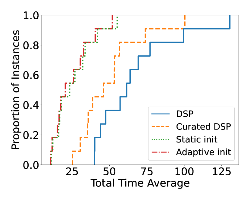
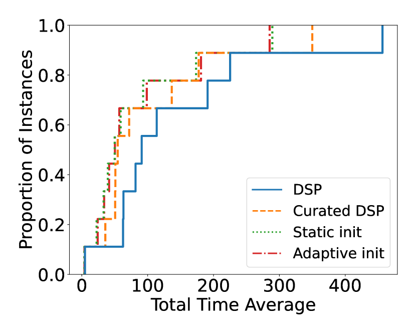
Tables 6 and 7 display the summary results of the different methods for solving the LP test instances for CFLP and CMND problems, respectively. The tables demonstrate the significant benefits of information reuse techniques for solving these test instances. The introduction of DSP drastically reduces SP count, suggesting that we are usually able to find violated cuts in the DSP, and only occasionally need to solve subproblems to generate cuts. This validates the presence of valuable dual solutions within the DSP, and their effectiveness in generating violated cuts. The reduction in SP count directly contributes to savings in SP T, leading to the observed savings in Total T. A somewhat surprising result is the decrease in iterations of the algorithm from baseline to DSP.
As hoped, we observe curated DSP reduces DSP T and hence leads to a reduction in Cut T and ultimately Total T. Intuitively, one might expect SP T to increase from DSP to curated DSP, as we have fewer dual solutions in the curated pool. However, the curation does not lead to a substantial increase in SP T suggesting that curated DSP obtains a good trade-off in the time saved from searching the DSP against the small extra time spent solving the subproblems
Both static and adaptive initialization methods consistently outperform baseline and DSP methods, needing significantly fewer iterations to converge. This shows the value of initializing the algorithm with Benders cuts. This reduction in iterations directly contributes to these methods having the shortest overall Total T. Interestingly, adaptive initialization needs the fewest iterations to converge. This suggests that it is able to identify useful cuts. However, we do not see proportional decrease in Total T because adaptive initialization needs more time to find these initial cuts. Also, adaptive initialization usually adds more cuts in the main problem, leading to longer time to solve the main problem. Overall, using the combination of information reuse methods we propose, we are able to solve these problems approximately 10 times faster compared to baseline on average.
We complement the summary results presented Tables 6 and 7 with the total time cumulative distribution function (CDF) plots shown in Figure 1. In these figures, the Y-axis shows the proportion of solved instances and the X-axis represents time. To focus on the relative improvements beyond just using DSP, these figures display only the four methods that reuse information and exclude the baseline method. Broadly, we observe that curated DSP improves significantly over DSP and that both initialization methods improve significantly over curated DSP, while they are comparable to each other.
4.3.2 IP Results
| Method | Total T | IP T | LP T | Cut T | DSP T | SP T | Init T |
|---|---|---|---|---|---|---|---|
| Baseline | 387.5 | 327.1 | 44.9 | 163.9 | - | 163.9 | 0.6 |
| DSP | 244.0 | 212.6 | 20.0 | 61.0 | 56.9 | 3.0 | 0.5 |
| Curated DSP | 216.9 | 191.4 | 14.7 | 46.2 | 41.4 | 3.8 | 0.5 |
| Static init | 194.1 | 182.4 | 6.1 | 43.9 | 39.2 | 3.8 | 0.6 |
| Adaptive init | 102.2 | 77.7 | 5.7 | 5.7 | 4.5 | 1.2 | 13.7 |
| Method | Total T | IP T | LP T | Cut T | DSP T | SP T | Init T |
|---|---|---|---|---|---|---|---|
| Baseline | 667.2 | 537.8 | 89.2 | 259.2 | - | 259.2 | 1.5 |
| DSP | 100.9 | 75.2 | 18.2 | 26.1 | 23.2 | 2.9 | 1.0 |
| Curated DSP | 61.8 | 45.8 | 9.8 | 10.5 | 7.0 | 3.4 | 1.0 |
| Static init | 58.5 | 47.2 | 6.5 | 9.4 | 6.3 | 2.9 | 1.1 |
| Adaptive init | 40.5 | 21.2 | 6.1 | 1.6 | 1.2 | 0.5 | 8.4 |
Tables 8 and 9 display the summary results of the different methods for solving the IP test instances for CFLP and CMND problems, respectively. We find that DSP reduces SP T which translates into savings in Total T. Curated DSP reduces the DSP T because of a smaller pool, in turn also helping to decrease Total T. Similar to the LP results, curated DSP does not lead to a significant increase in SP T, suggesting that curated DSP provides a good trade-off in the time checking the DSP against the time spent solving subproblems.
The static and adaptive initialization methods consistently outperform baseline and DSP techniques. While the two initialization methods performed comparably for LPs, we see a clear distinction for IPs. For CFLP, static initialization offers only a marginal improvement over curated DSP, whereas adaptive initialization demonstrates a substantial two-fold improvement in total time and a ten-fold reduction in cut generation time. This highlights the effectiveness of adaptive initialization in identifying strong initial cuts. Data for CMND shows a similar trend, with adaptive initialization again proving superior and static initialization providing only a marginal benefit over curated DSP. Although adaptive initialization has a higher initial computational cost (Init T), it delivers superior overall performance (Total T), making it the best choice for IPs.
| Method | Nodes | Root gap (%) | Callback calls | SP count |
|---|---|---|---|---|
| Baseline | 2814.5 | 2.9 | 115.7 | 115.7 |
| DSP | 2819.9 | 3.1 | 116.6 | 6.1 |
| Curated DSP | 2824.7 | 3.1 | 114.8 | 6.6 |
| Static init | 2645.7 | 3.1 | 111.0 | 6.5 |
| Adaptive init | 2129.8 | 2.8 | 13.4 | 1.9 |
| Method | Nodes | Root gap (%) | Callback calls | SP count |
|---|---|---|---|---|
| Baseline | 2404.9 | 12.7 | 140.1 | 140.1 |
| DSP | 1446.1 | 11.6 | 71.2 | 5.0 |
| Curated DSP | 1357.7 | 11.2 | 64.5 | 5.5 |
| Static init | 1420.7 | 9.3 | 62.5 | 5.2 |
| Adaptive init | 1379.0 | 3.9 | 10.8 | 1.2 |
Tables 10 and 11 present results of additional metrics for these instances. We observe a significant reduction in the SP count after employing DSP, similar to what we saw for LPs. Interestingly, deploying adaptive initialization leads to a significant reduction in both the callback calls and SP count compared to other methods. This suggests that the initial cuts generated by adaptive initialization provide a strong relaxation of the original problem, minimizing the need for looking for additional cuts during the optimization process. Furthermore, adaptive initialization improves root gaps, particularly for CMND. Since root gaps help isolate the impact of initialization, this demonstrates that adaptive initialization closes the most gap among all methods. The resulting reduction in callback calls confirms that the initial cuts are highly effective.
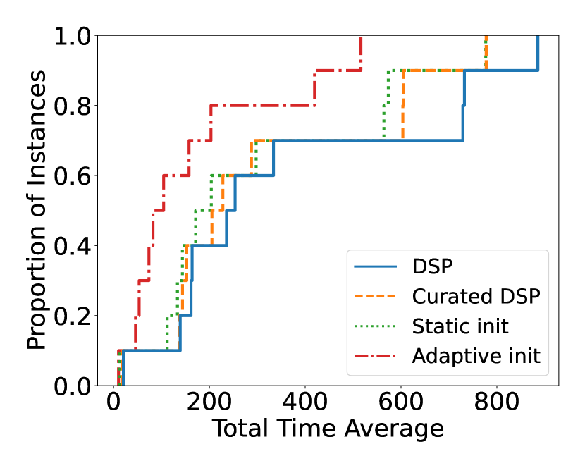
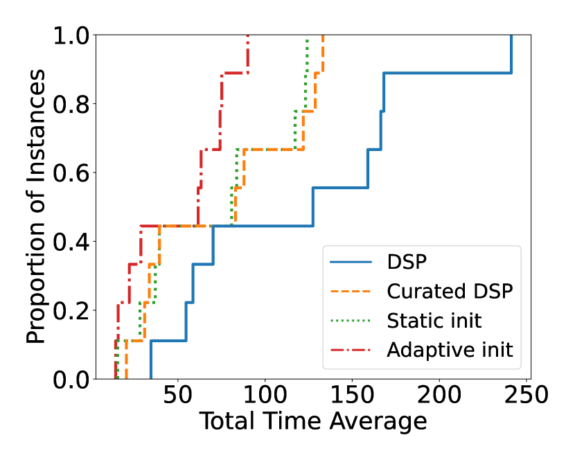
Figure 2 presents the cumulative distribution function (CDF) plots of solution times for IP instances, again displaying the results only for the methods that reuse information. These plots further illustrate that the adaptive initialization method has the best performance. We also see that curated DSP generally leads to an improvement in total time compared to regular DSP.
4.3.3 Cut Distribution
| Method | Initial cuts | SP cuts | DSP cuts | Total cuts |
|---|---|---|---|---|
| Baseline | - | 39192 | - | 39192 |
| DSP | - | 448 | 33455 | 33903 |
| Curated DSP | - | 589 | 34139 | 34728 |
| Static Init | 784 | 608 | 33327 | 34719 |
| Adaptive Init | 13105 | 128 | 3610 | 16843 |
| Method | Initial cuts | SP cuts | DSP cuts | Total cuts |
|---|---|---|---|---|
| Baseline | - | 55721 | - | 55721 |
| DSP | - | 85 | 29851 | 29936 |
| Curated DSP | - | 128 | 27604 | 27732 |
| Static Init | 782 | 50 | 26455 | 27287 |
| Adaptive Init | 8723 | 24 | 3629 | 12376 |
Our algorithm generates Benders cuts from three sources: cuts provided during initialization (Initial cuts), cuts derived by solving subproblems during the algorithm (SP cuts), and cuts obtained by searching a pool of dual solutions (DSP cuts). To provide more insight about our methods, we present in Tables 12 and 13 the distribution of cuts of each type for a sample IP instance of the CFLP and CMND problems, respectively. To focus on differences between the methods, the Initial cuts and Total cuts exclude active LP cuts, which are nearly identical for all methods.
We find that the inclusion of DSP in the Benders decomposition framework significantly reduces the number of subproblems solved to generate cuts, leading to a dramatic decrease in SP cuts. This is expected and confirms the presence of useful dual solutions within the pool, capable of generating violated cuts. We also find that curated DSP requires slightly more SP cuts than DSP, which can be attributed to the reduced size of the curated DSP compared to the DSP. Using either of the initialization methods leads to a further reduction in the number of subproblem solves required to generate cuts relative to the curated DSP. Finally, we observe a drastic reduction in the number of total cuts needed to reach the optimal solution when using adaptive initialization, which is explained by the significant decrease in the number of cuts added from the DSP. The adaptive initialization method requires very few additional cuts beyond the initial set introduced during problem initialization. This translates to significant time savings in solving the SAA replication.
4.3.4 Impact of Adaptive Initialization
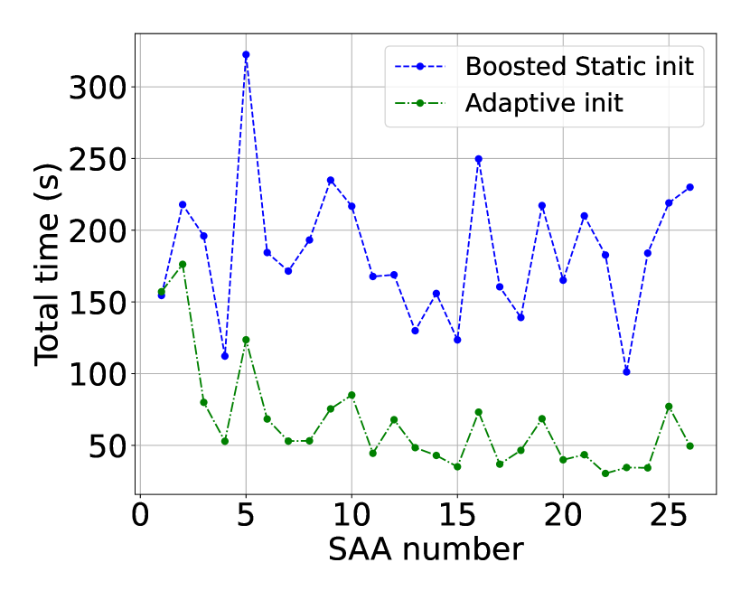
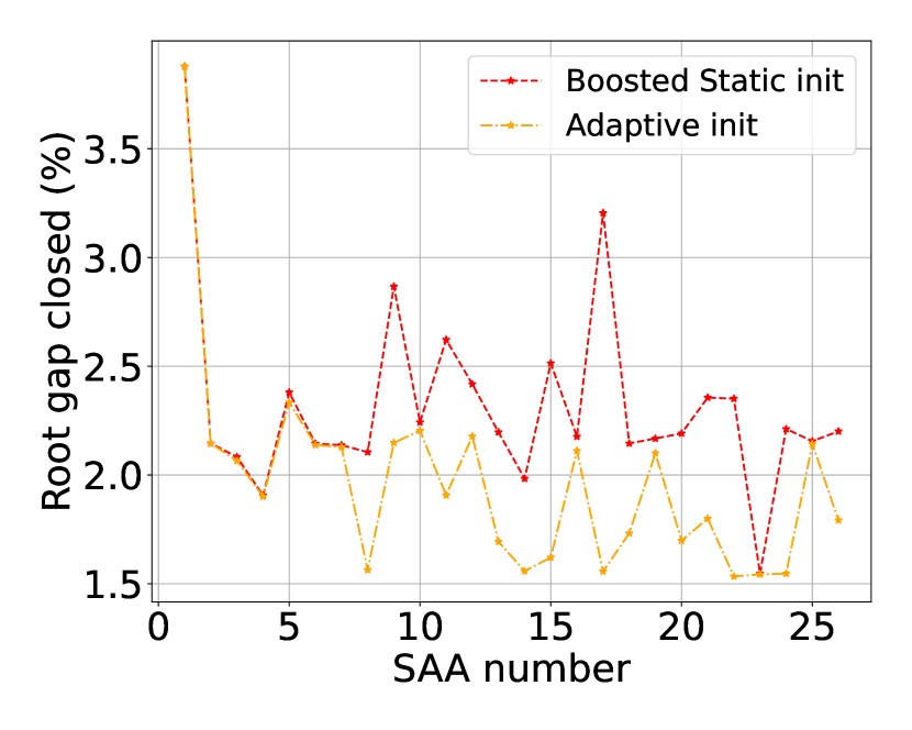
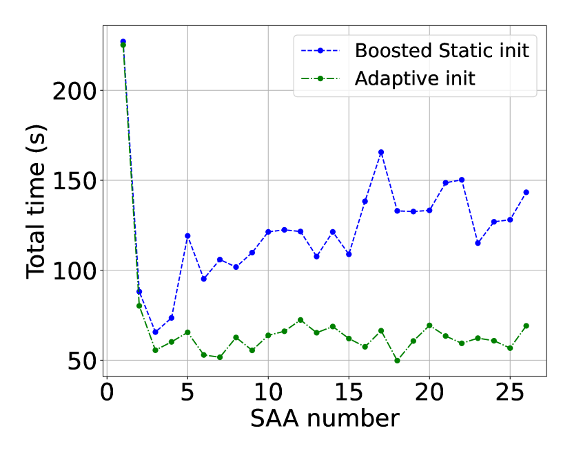
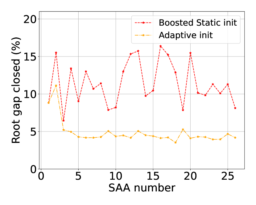
Analysis of the cut distribution in Tables 12 and 13 reveals that adaptive initialization consistently introduces a higher number of initial cuts compared to static initialization. To isolate the impact of cut quality from quantity on the observed performance improvements, we conduct another experiment in which we modify the static initialization method to add the same number of cuts as adaptive initialization. In this version of static initialization, which we refer to as boosted static initialization, we solve the LP relaxation first as usual, and then use static initialization to add cuts per scenario to the main problem, where is the number of cuts that was added by the adaptive initialization method for the same instance. For each scenario within the new SAA replication, we identify the top dual solutions from the DSP that lead to the highest value of the subproblem objective value function, , evaluated at the first two optimal solutions in . The cuts generated from these are then used to initialize the problem. This ensures both initialization approaches use the same number of cuts.
In Fig. 3, we track the root node gap closed and also the average time taken to solve the SAA replication over 26 replications using boosted static initialization and adaptive initialization. The results demonstrate that adaptive initialization remains superior even when the static initialization adds the same number of cuts. Thus, we conclude that the adaptive nature of adaptive initialization is important, and in particular it seems to benefit from allowing the number of cuts added for each scenario to vary.
4.3.5 Impact of Curated DSP
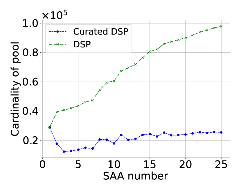
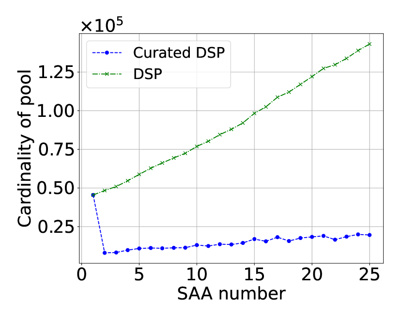
In Figure 4, we plot the size of the DSP and curated DSP as we solve more SAA replications. For CMND, we notice that, the DSP constantly increases in size, but the curated DSP has a sharp decrease in size in the second replication. Although it begins to grow again after that, the increase is not as significant compared to the DSP. This indicates that we have successfully achieved our goal for the curated DSP, as we are able to maintain a controlled size of the pool. In the case of CFLP, we notice similar trends, although the reduction in size from the first to the second replication is not as pronounced as in CMND. Additionally, by the end of the 25 replications, the size of the pool is nearly the same as it was after the first replication.
We next investigate the importance of our particular mechanism for choosing the dual solutions to keep in the curated DSP. To do this, we compared our method to a baseline that randomly selects the same number of dual solutions as were chosen in our curated DSP method. We refer to this method as the random curated DSP.
| Method | CFLP | CMND |
|---|---|---|
| Curated DSP | 153.17 | 89.56 |
| Random curated DSP | 152.28 | 92.19 |
In Table 14, we display the average total time taken to solve 25 SAA replications after the first one with these two methods. We use the same instances to test these methods as the experiments on cut distribution in Sec. 4.3.3. The results indicate that there is no significant improvement in time using our curated DSP method compared to a random curated DSP. Thus, we find that the key feature of the curated DSP that explains its performance is the reduction of the size of the DSP – the particular choice of the dual solutions that are kept does not outperform a random choice. Thus, the key feature of our method is that it suggests the number of dual solutions to retain in the curated DSP without requiring this number as input.
4.3.6 Performance with Varying Number of Scenarios
All the previous experiments have been done on instances in which the number of scenarios in each replication is 400. We next investigate the impact of varying the number of scenarios in the replications on our conclusions.
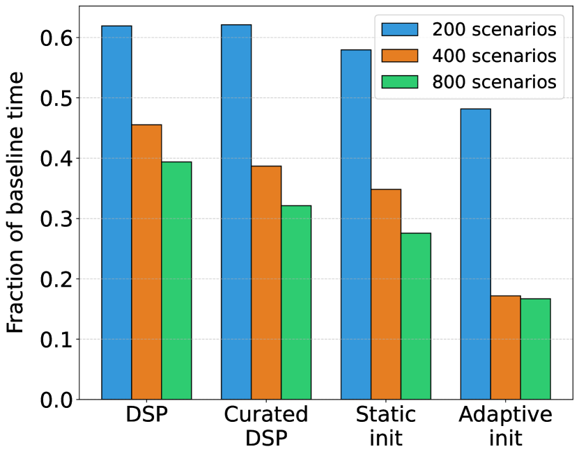
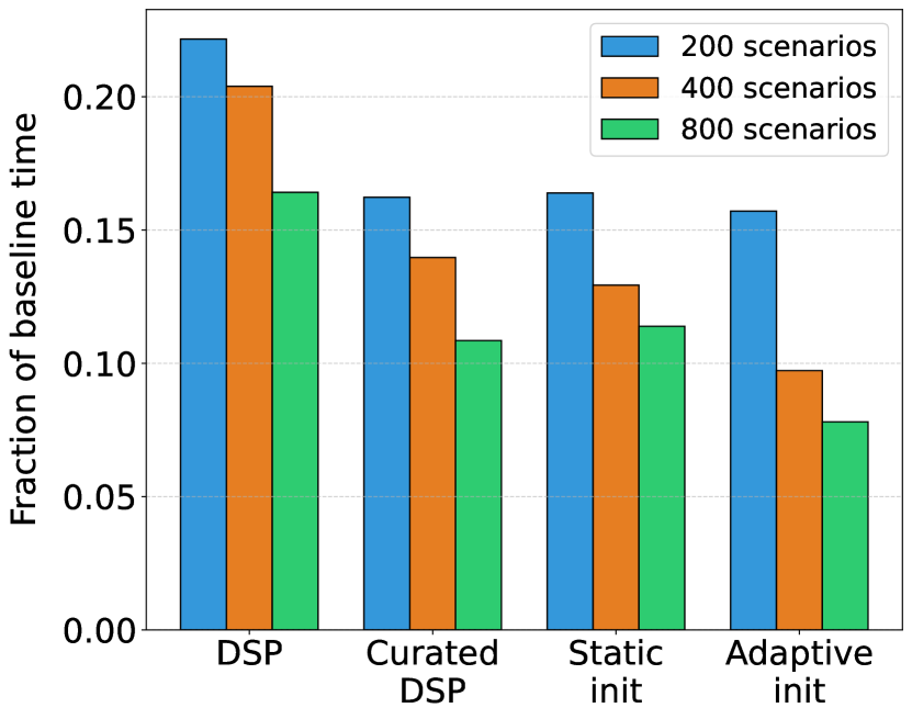
For this experiment, we select one instance for each problem class and then run our methods for that instance with the number of scenarios as 200, 400, and 800. For network design, we use instance r09.2 for the LP case and r03.3 for the IP case For facility location, we select the instance with 55 facilities and 495 customers for LP, while the IP instance has 35 facilities and 105 customers.
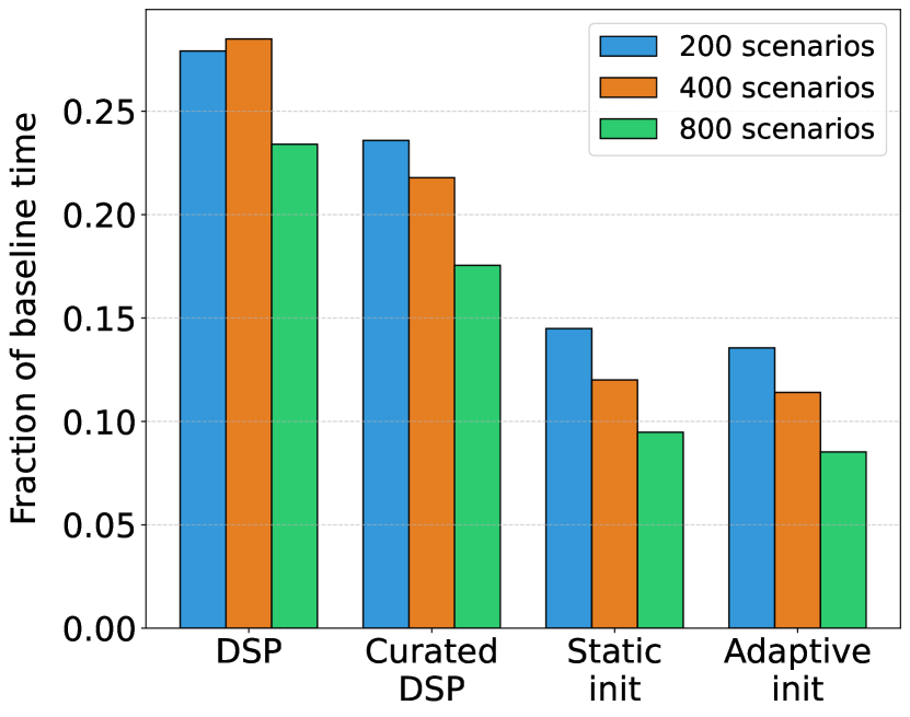
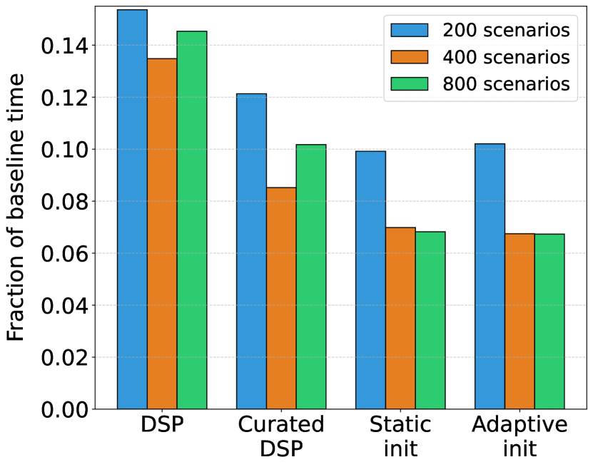
Figure 5 displays the relative performance of our information reuse methods as a fraction of the execution time of the baseline method, across three scenario sets. We find that in general the relative performance of the different methods is similar across the different scenario sizes. We also find that the improvements from reusing information tend to be more significant for instances with more scenarios, which is not surprising considering that in such instances there is more work that has to be done in solving subproblems, and hence more opportunity to save time on that work with the proposed DSP and initialization techniques.
5 Conclusion and Future Directions
We presented methods to accelerate solving a sequence of SAA replications in two-stage stochastic programming, assuming randomness only in the right-hand sides of the subproblems. These methods are derived for Benders decomposition as the solution algorithm and we find that, for our test problems, it is possible to reduce the time to solve the replications after the first one by a factor of 10 for both stochastic LP and IP problems by using the information reuse techniques we have proposed.
One significant direction for future research is to consider problems in which the subproblems have uncertainty in either the objective coefficients or the recourse matrix. Such problems do not have the property that the dual feasible region is fixed across scenarios, and hence the techniques we proposed do not extend directly to such problems.
This paper focused on the Benders decomposition algorithm, as it is a leading algorithm for both two-stage stochastic LPs and for IPs with continuous recourse. Future research could investigate techniques for accelerating different algorithms in this context of solving a sequence of SAA replications. For example, for two-stage stochastic LPs, the level method lemarechal1995new ; fabian2007solving often performs better than Benders decomposition. We anticipate that the techniques presented here would be useful for accelerating this and other cut-based decomposition methods, but testing this hypothesis would be an interesting direction for future work. It would also be interesting to explore methods to accelerate alternative methods for solving two-stage stochastic IPs, such as dual decomposition caroe1999dual and methods that use different types of cuts boland2018combining ; chen2022generating ; gade2014decomposition ; lulli2004branch ; rahmaniani2017benders ; van2020converging .
References
- (1) Adulyasak, Y., Cordeau, J.F., Jans, R.: Benders decomposition for production routing under demand uncertainty. Operations Research 63(4), 851–867 (2015)
- (2) Bayraksan, G., Morton, D.P.: Assessing solution quality in stochastic programs. Mathematical Programming 108, 495–514 (2006)
- (3) Benders, J.: Partitioning procedures for solving mixed-variables programming problems. Numerische Mathematik 4, 238–252 (1962). URL https://doi.org/10.1007/BF01386316
- (4) Bengio, Y., Frejinger, E., Lodi, A., Patel, R., Sankaranarayanan, S.: A learning-based algorithm to quickly compute good primal solutions for stochastic integer programs. In: Integration of Constraint Programming, Artificial Intelligence, and Operations Research: 17th International Conference, CPAIOR 2020, Vienna, Austria, September 21–24, 2020, Proceedings 17, pp. 99–111. Springer (2020)
- (5) Bengio, Y., Lodi, A., Prouvost, A.: Machine learning for combinatorial optimization: a methodological tour d’horizon. European Journal of Operational Research 290(2), 405–421 (2021)
- (6) Birge, J.R., Louveaux, F.: Introduction to stochastic programming. Springer Science & Business Media (2011)
- (7) Boland, N., Christiansen, J., Dandurand, B., Eberhard, A., Linderoth, J., Luedtke, J., Oliveira, F.: Combining progressive hedging with a Frank–Wolfe method to compute Lagrangian dual bounds in stochastic mixed-integer programming. SIAM Journal on Optimization 28(2), 1312–1336 (2018)
- (8) Borozan, S., Giannelos, S., Falugi, P., Moreira, A., Strbac, G.: Machine learning-enhanced benders decomposition approach for the multi-stage stochastic transmission expansion planning problem. Electric Power Systems Research 237, 110985 (2024). DOI https://doi.org/10.1016/j.epsr.2024.110985. URL https://www.sciencedirect.com/science/article/pii/S0378779624008708
- (9) Carøe, C.C., Schultz, R.: Dual decomposition in stochastic integer programming. Operations Research Letters 24(1-2), 37–45 (1999)
- (10) Chan, T., Lin, B., Saxe, S.: A machine learning approach to solving large bilevel and stochastic programs: Application to cycling network design. Available at SSRN 4592562 (2023)
- (11) Chen, R., Luedtke, J.: On generating lagrangian cuts for two-stage stochastic integer programs. INFORMS Journal on Computing 34(4), 2332–2349 (2022)
- (12) Cornuéjols, G., Sridharan, R., Thizy, J.M.: A comparison of heuristics and relaxations for the capacitated plant location problem. European journal of operational research 50(3), 280–297 (1991)
- (13) Crainic, T.G., Fu, X., Gendreau, M., Rei, W., Wallace, S.W.: Progressive hedging-based metaheuristics for stochastic network design. Networks 58(2), 114–124 (2011)
- (14) Deza, A., Khalil, E.B.: Machine learning for cutting planes in integer programming: A survey. arXiv preprint arXiv:2302.09166 (2023)
- (15) Dumouchelle, J., Patel, R., Khalil, E.B., Bodur, M.: Neur2sp: Neural two-stage stochastic programming. arXiv preprint arXiv:2205.12006 (2022)
- (16) Dupačová, J., Popela, P.: Melt control: Charge optimization via stochastic programming. In: Applications of stochastic programming, pp. 277–297. SIAM (2005)
- (17) Dyer, M., Stougie, L.: Computational complexity of stochastic programming problems. mathematical programming 106, 423–432 (2006)
- (18) Fábián, C.I., Szőke, Z.: Solving two-stage stochastic programming problems with level decomposition. Computational Management Science 4, 313–353 (2007)
- (19) Fortz, B., Poss, M.: An improved benders decomposition applied to a multi-layer network design problem. Operations research letters 37(5), 359–364 (2009)
- (20) Gade, D., Küçükyavuz, S., Sen, S.: Decomposition algorithms with parametric Gomory cuts for two-stage stochastic integer programs. Mathematical Programming 144(1-2), 39–64 (2014)
- (21) Ghamlouche, I., Crainic, T.G., Gendreau, M.: Cycle-based neighbourhoods for fixed-charge capacitated multicommodity network design. Operations research 51(4), 655–667 (2003)
- (22) Higle, J.L., Sen, S.: Stochastic decomposition: An algorithm for two-stage linear programs with recourse. Mathematics of operations research 16(3), 650–669 (1991)
- (23) Jia, H., Shen, S.: Benders cut classification via support vector machines for solving two-stage stochastic programs. INFORMS Journal on Optimization 3(3), 278–297 (2021)
- (24) Kim, S., Pasupathy, R., Henderson, S.G.: A guide to sample average approximation. Handbook of simulation optimization pp. 207–243 (2015)
- (25) Kleywegt, A.J., Shapiro, A., Homem-de Mello, T.: The sample average approximation method for stochastic discrete optimization. SIAM Journal on optimization 12(2), 479–502 (2002)
- (26) Lam, H., Qian, H.: Bounding optimality gap in stochastic optimization via bagging: Statistical efficiency and stability. arXiv preprint arXiv:1810.02905 (2018)
- (27) Larsen, E., Frejinger, E., Gendron, B., Lodi, A.: Fast continuous and integer l-shaped heuristics through supervised learning. INFORMS Journal on Computing (2023)
- (28) Lee, M., Ma, N., Yu, G., Dai, H.: Accelerating generalized benders decomposition for wireless resource allocation. IEEE Transactions on Wireless Communications 20(2), 1233–1247 (2020)
- (29) Lemaréchal, C., Nemirovskii, A., Nesterov, Y.: New variants of bundle methods. Mathematical programming 69, 111–147 (1995)
- (30) Lulli, G., Sen, S.: A branch-and-price algorithm for multistage stochastic integer programming with application to stochastic batch-sizing problems. Management Science 50(6), 786–796 (2004)
- (31) Mak, W.K., Morton, D.P., Wood, R.K.: Monte carlo bounding techniques for determining solution quality in stochastic programs. Operations research letters 24(1-2), 47–56 (1999)
- (32) Mitrai, I., Daoutidis, P.: Learning to initialize generalized benders decomposition via active learning. FOCAPO/CPC, San Antonio, Texas (2023)
- (33) Mitrai, I., Daoutidis, P.: Computationally efficient solution of mixed integer model predictive control problems via machine learning aided benders decomposition. Journal of Process Control 137, 103207 (2024)
- (34) Nair, V., Dvijotham, D., Dunning, I., Vinyals, O.: Learning fast optimizers for contextual stochastic integer programs. In: UAI, pp. 591–600 (2018)
- (35) Naoum-Sawaya, J., Elhedhli, S.: An interior-point benders based branch-and-cut algorithm for mixed integer programs. Annals of Operations Research 210, 33–55 (2013)
- (36) Rahmaniani, R., Crainic, T.G., Gendreau, M., Rei, W.: The benders decomposition algorithm: A literature review. European Journal of Operational Research 259(3), 801–817 (2017)
- (37) Saharidis, G.K., Boile, M., Theofanis, S.: Initialization of the benders master problem using valid inequalities applied to fixed-charge network problems. Expert Systems with Applications 38(6), 6627–6636 (2011)
- (38) Sakhavand, N., Gangammanavar, H.: Subproblem sampling vs. scenario reduction: efficacy comparison for stochastic programs in power systems applications. Energy Systems pp. 1–29 (2022)
- (39) Sen, S., Doverspike, R.D., Cosares, S.: Network planning with random demand. Telecommunication systems 3(1), 11–30 (1994)
- (40) Sen, S., Liu, Y.: Mitigating uncertainty via compromise decisions in two-stage stochastic linear programming: Variance reduction. Operations Research 64(6), 1422–1437 (2016)
- (41) Song, Y., Luedtke, J.R., Küçükyavuz, S.: Chance-constrained binary packing problems. INFORMS Journal on Computing 26(4), 735–747 (2014)
- (42) van der Laan, N., Romeijnders, W.: A converging Benders’ decomposition algorithm for two-stage mixed-integer recourse models. Operations Research 72, 2190–2214 (2023)
- (43) Van Slyke, R.M., Wets, R.: L-shaped linear programs with applications to optimal control and stochastic programming. SIAM journal on applied mathematics 17(4), 638–663 (1969)
- (44) Wang, S., Gangammanavar, H., Ekşioğlu, S., Mason, S.J.: Statistical estimation of operating reserve requirements using rolling horizon stochastic optimization. Annals of Operations Research 292, 371–397 (2020)
Appendix A
We provide detailed descriptions of the problems considered in our computational study. We adopt the formulations and problem descriptions from jia2021benders for both test problems.
A.1 Capacitated Facility Location Problem
Consider a set of facilities, where a facility has a setup cost and a production capacity limit . Additionally consider a set of customers , where each customer has an uncertain demand denoted by . The vector of realizations of this uncertain demand in a scenario is denoted by . This demand can be met by shipping from any open facility to customer at a unit transportation cost . Any unmet demand for customer incurs a lost-sale penalty, with a unit cost . The objective is to select a subset of facilities to open in order to minimize the total expected cost.
This problem is modeled as a two-stage stochastic programming problem. The first-stage binary decision variables indicate whether the facility is opened or not. In the second-stage, after revelation of the demands, we introduce continuous decision variables , which represent goods transported from facility to customer . The model aims to find the best decisions to minimize the sum of facility setup cost, expected transportation cost, and expected lost-sale cost. The first-stage formulation is given by:
| s.t. |
The second-stage problem for each scenario , is defined using transportation variables from a facility to a customer and auxiliary variables that denote the amount of unmet demand of customer . We have:
| subject to | ||||
By allowing unmet demand, the problem always has a feasible solution and Benders decomposition only requires optimality cuts.
A.2 Multi Commodity Network Design Problem
Consider a directed network with node set , arc set , and commodity set . Each commodity has an uncertain demand that must be routed from an origin node, , to its destination node, . The vector of demands in scenario is denoted by . For each arc , there is an installation cost and an arc capacity . The cost for transporting one unit of commodity on installed arc is . Any demand that is not met is penalized at a rate of per unit.
The objective in the first-stage is to decide which subset of arcs to install to minimize the sum of arc installation cost and expected total transportation cost and penalty for unmet demand. In the second-stage, after demand is realized, the goal is to determine the optimal flow of commodities through the installed arcs to minimize the sum of transportation and unmet demand costs.
In the first-stage, we define binary decisions for all arcs such that if we install arc . The first-stage formulation is given by:
In the second-stage, we define non-negative continuous decisions to represent transportation units of commodity on arc . Additionally, we introduce auxiliary variables to denote the unmet demand for commodity . For scenario , the formulation is given by:
| subject to | ||||
The parameter is set to if node is the origin of the commodity if node is the destination of the commodity , or 0 otherwise. By allowing unmet demand, the problem always has a feasible solution and Benders decomposition only requires optimality cuts.