Discrete Curvature on Graphs

In this paper we address the reverse isoperimetric inequality for convex bodies with uniform curvature constraints in the hyperbolic plane $\mathbb{H}^{2}$. We prove that the thick $\lambda$-sausage body, that is, the convex domain bounded by two equal circular arcs of curvature $\lambda$ and two equal arcs of hypercircle of curvature $1/\lambda$, is the unique minimizer of area among all bodies $K\subset\mathbb{H}^{2}$ with a given length and with curvature of $\partial K$ satisfying $1/\lambda\leq\kappa\leq\lambda$ (in a weak sense). We call this class of bodies thick $\lambda$-concave bodies, in analogy to the Euclidean case where a body is $\lambda$-concave if $0\leq\kappa\leq\lambda$. The main difficulty in the hyperbolic setting is that the inner parallel bodies of a convex body are not necessarily convex. To overcome this difficulty, we introduce an extra assumption of thickness $\kappa\geq 1/\lambda$.
In addition, we prove the Blaschke’s rolling theorem for $\lambda$-concave bodies under the thickness assumption. That is, we prove that a ball of curvature $\lambda$ can roll freely inside a thick $\lambda$-concave body. In striking contrast to the Euclidean setting, Blaschke’s rolling theorem for $\lambda$-concave domains in $\mathbb{H}^{2}$ does not hold in general, and thus has not been studied in literature before. We address this gap, and show that the thickness assumption is necessary and sufficient for such a theorem to hold.

Keywords: reverse isoperimetric inequality, $\lambda$-concavity, $\lambda$-convexity, hyperbolic plane, Blaschke’s rolling theorem

MARIA ESTEBAN

Abstract

1 Introduction

The reverse isopermietric problem is inspired from the classical isoperimetric problem which has been thoroughly studied in the past and generalized in a variety of contexts (see [1]). The classical problem concerns about finding the body with the largest volume for a given surface area. In $\mathbb{R}^{n}$ it is well known that the solution is an $n$-dimensional ball. The reverse isoperimetric problem addresses the opposite case. That is, it searches for the body that minimizes the volume for a given surface area. This problem has a trivial solution as, for a given surface area, the $n$-dimensional volume can be arbitrary small (the flat pancake problem [2]).

To avoid this degeneration, in this paper we restrict the reverse isoperimetric problem to convex bodies with uniform curvature constraints. Our focus will be on bodies lying in the hyperbolic plane $\mathbb{H}^{2}$, which we assume has constant curvature of -$1$. In particular, we look at convex bodies $K\subset\mathbb{H}^{2}$ whose boundary curvature satisfies $1/\lambda\leq\kappa\leq\lambda$, in a weak sense (see below). We call these thick $\lambda$-concave bodies. Recall that a convex body is a closed convex set with non-empty interior. This restricts the body from being too flat or too curved.

1.1 Some reverse isoperimetric results

In this paper, we focus on $\lambda$-concave and $\frac{1}{\lambda}$-convex bodies. Throughout, we assume that $\lambda>1$ and that the normal to the boundary $\partial K$ of a convex body $K$ points in the direction of convexity.

Definition 1 ($\lambda$-convex and $\lambda$-concave bodies [3]).

A convex body $K\subset\mathbb{H}^{2}$ is $\lambda$-convex if for each $x\in\partial K$ there exists a neighborhood $U_{x}\subset\mathbb{H}^{2}$ and a closed curve of constant curvature $\partial S_{\lambda}$ (see Section 2.1) such that

$$U_{x}\cap\partial K\subset S_{\lambda}$$

where $S_{\lambda}$ is the convex region bounded by $\partial S_{\lambda}$. Similarly, $K$ is $\lambda$-concave if for each $x\in\partial K$ there exists a neighborhood $U_{x}\subset\mathbb{H}^{2}$ such that

$$U_{x}\cap\partial S_{\frac{1}{\lambda}}\subset K$$

Equivalently, if $\partial K$ is $C^{2}$-smooth then $K$ is $\lambda$-convex if for all $x\in\partial K$ the geodesic curvature $k(x)\geq\lambda$, and $\lambda$-concave if for all $x\in\partial K$ the geodesic curvature $0\leq k(x)\leq\lambda$.

Some results on the isoperimetric problem of $\lambda$-convex and $\lambda$-concave bodies have already been obtained in $\mathbb{R}^{n}$.

• The Reverse Isoperimetric Inequality for $\lambda$-concave Bodies ([4], see also [5, 6]). Let $n\geq 2$. Let $K\subset\mathbb{R}^{n}$ be a $\lambda$-concave body, and let $S\subset\mathbb{R}^{n}$ be a $\lambda$-sausage, i.e., the convex hull of two balls of radius $1/\lambda$. If $|\partial K|=|\partial S|$, then $|K|\geq|S|$, and equality holds if and only if $K$ is a $\lambda$-sausage.

Less is known for $\lambda$-convex bodies in $\mathbb{R}^{n}$.The following conjecture was formulated by Borisenko (see [4]):

• Conjecture: The Reverse Isoperimetric Inequality for $\lambda$-convex bodies in $\mathbb{R}^{n}$. Let $n\geq 2$. Let $K\subset\mathbb{R}^{n}$ be a $\lambda$-convex body, and let $L\subset\mathbb{R}^{n}$ be a $\lambda$-convex lens, i.e., the intersection of two balls of radius $1/\lambda$. If $|\partial K|=|\partial L|$, then $|K|\geq|L|$, and equality holds if and only if $K$ is a $\lambda$-convex lens.

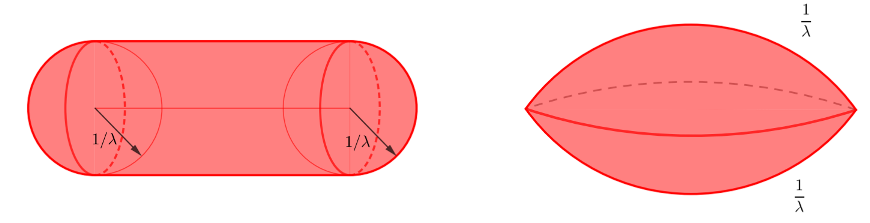
Figure 1: $\lambda$-sausage (left) and $\lambda$-convex lens (right) [4]

For $n=2$ the conjecture was proved by [7] (see [8] for alternative proof). For $n=3$ the conjecture was proved in [3]. In this paper, we also address the Blaschke’s Rolling Theorem for thick $\lambda$-concave bodies. The statement of the classical result is as follows:

• Theorem: Blaschke’s Rolling Theorem [9]. Let $\gamma$ be a closed, smooth, convex curve in $\mathbb{R}^{2}$ such that for all $x\in\gamma,\,\kappa(x)\leq\lambda$. Then, a ball of curvature $\lambda$ rolls freely inside.

This result was extended in $\mathbb{R}^{n}$ by [10, 11], and later on in Riemannian manifolds of bounded curvature by [12, 13, 14, 15]. Nevertheless, this theorem does not hold in general for $\lambda$-concave domains in $\mathbb{H}^{2}$, and hence was never studied in literature before. We fix this gap by providing a Blaschke’s Rolling Theorem for $\lambda$-concave bodies under the thickness condition (Theorem C). We also show that this result is optimal.

1.2 Reverse isoperimetric inequality in $\mathbb{H}^{2}$

We will first define the main object of interest in this paper, the thick $\lambda$-sausage:

Definition 2 (Thick $\lambda$-sausage).

A thick $\lambda$-sausage is the convex domain bounded by two equal circular arcs of curvature $\lambda$ and two equal arcs of hypercircle of curvature $1/\lambda$ (see Figure 2).

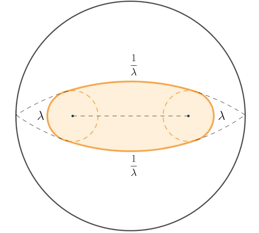
Figure 2: Thick $\lambda$-sausage

In this paper we provide a proof of the theorems stated below. Note that given $K\subset\mathbb{H}^{2}$, $|\partial K|$ refers to the length of the boundary $\partial K$ and $|K|$ to the area of $K$.

Theorem A.

(Reverse isoperimetric inequality for thick $\lambda$-concave bodies in $\mathbb{H}^{2}$) Let $K\subset\mathbb{H}^{2}$ be a thick $\lambda$-concave body and let $S\subset\mathbb{H}^{2}$ be a thick $\lambda$-sausage, as in Definition (2). If $|\partial K|=|\partial S|$, then $|K|\geq|S|$. Moreover, equality holds if and only if $K$ is a thick $\lambda$-sausage.

Theorem B.

(Lower bound for reverse isoperimetric inequality for thick $\lambda$-concave bodies in $\mathbb{H}^{2}$) Let $K\subset\mathbb{H}^{2}$ be a thick $\lambda$-concave body. Then,

$$|K|\geq\frac{|\partial K|}{\lambda}+2\pi\left(1-\sqrt{1-\frac{1}{\lambda^{2}}}\right).$$

Moreover, equality holds if and only if $K$ is a thick $\lambda$-sausage.

Remark: In fact, if $K\subset\mathbb{H}^{2}(-c^{2})$ is a thick $\lambda$-concave body, then,

$$|K|\geq\frac{|\partial K|}{\lambda}+\frac{2\pi}{c^{2}}\left(1-\sqrt{1-\frac{c^{2}}{\lambda^{2}}}\right).$$

And, as $c\rightarrow 0$, the inequality approaches the classical Euclidean result in $\mathbb{R}^{2}$ proved in [4] (this inequality complements the analogous results in $\mathbb{S}^{2}$ [16])

Theorem C.

(Blaschke’s rolling theorem for $\lambda$- concave bodies) Let $K\subset\mathbb{H}^{2}$ is a thick $\lambda$-concave body. Then the ball of curvature $\lambda$ can roll freely in $K$. Moreover, for every $\lambda^{\prime}>\lambda$, there exists a closed convex curve with $1/\lambda^{\prime}\leq k\leq\lambda$ such that a disk of radius $R=\coth^{-1}(\lambda)$ can not roll freely in the domain bounded by the curve.

1.3 Structure of the paper

In Section 2, we provide some background information on the curvature of convex bodies in the hyperbolic plane. In Section 3 we give the proof of Theorem A, which is divided into three steps for clarity. The proof follows a similar approach than in the Euclidean case, where the structure of the inner parallel bodies is analyzed, but with the additional difficulty than in the hyperbolic plane the inner parallel body of a convex body is not necessarily convex. The proof of Theorem B and Theorem C will mostly follow from Theorem A.

1.4 Acknowledgements

I would like to express my gratitude to Kostiantyn Drach for supervising this project as part of the Barcelona Introduction to Mathematical Research 2024 (BIMR) summer program, organized by the Centre de Recerca Matemàtica (CRM).

2 Background Theory

2.1 Curves of constant curvature in $\mathbb{H}^{2}$

In the Hyperbolic Space of curvature -$1$ there are multiple types of curves of constant geodesic curvature (see Figure 3). This section provides the definition and properties of such curves (see e.g [17] or [3]).

• Circles: Circles of radius $R$ have geodesic curvature $\lambda=\lambda=\coth(R)>1$. Both in the Poincaré Disk Model and in the Upper Half-Plane Model, hyperbolic circles are Euclidean circles, even though, in general, the hyperbolic center does not coincide with the Euclidean center of the disk.

• Geodesics: The geodesic curvature of geodesics is 0. In the Poincaré Disk Model, geodesics appear as arcs of circles that are orthogonal to the boundary of the disk or as straight lines passing through the center. In the Upper Half-Plane Model, geodesics are represented as either semicircles orthogonal to the boundary (the real line) or vertical lines perpendicular to the boundary.

• Horocyles: A horocycle is a curve whose perpendicular geodesics converge asymptotically to the same direction. Horocyles have geodesic curvature $\lambda=1$. In the Poincaré Disk Model, horocycles appear as Euclidean circles that are tangent to the boundary of the disk. The center of the horocyle is an ideal point (lies on the boundary of the Hyperbolic space) and has “infinite radius”. In the Upper Half-Plane model, horocycles appear as Euclidean circles tangent to the real line or as horizontal lines.

• Hypercircles: Hypercircles are curves equidistant to a geodesic. They have a geodesic curvature $\lambda\in(0,1)$. In the Poincaré Disk Model and Upper Half-Plane model, a hypercircle appears as an arc of a Euclidean circle that intersects the boundary of the model at two distinct points with an angle $0<\alpha<\frac{\pi}{2}$.

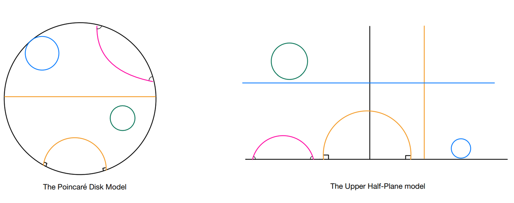
Figure 3: Hyperbolic (green), Geodesics (orange), Horocycles (blue) and Hypercircles (pink)

2.2 Some useful lemmas

Lemma 2.1.

In the Poincaré Disk Model, the geodesic curvature of a curve at (0,0) is $\frac{1}{2}$ of its Euclidean curvature at that point.

Proof.

The Poincaré metric in the unit disk $x^{2}+y^{2}<1$ is $ds^{2}=\frac{4\left(dx^{2}+dy^{2}\right)}{\left(1-x^{2}-y^{2}\right)^{2}}$. To calculate the geodesic curvature of a curve through (0,0), we use the parallel transport to quantify how much does the curve curve with respect to the geodesic, which in this case is the diameter of the circle. Near the center, its arclength parametrization is approximately $(\frac{t}{2},0)$ for $t\rightarrow 0$. Hence, the parallel transport along this geodesic for small distances near center will be Euclidean and the geodesic curvature at that point will be just $\frac{1}{2}$ of its Euclidean curvature at that point. ∎

Lemma 2.2.

Let $\beta$ be the angle between the hypercicle and the boundary of the of the unit disk in the Poincaré Disk Model, as seen in Figure 4. Then, the curvature $\lambda$ of an hypercircle $\Gamma\subset\mathbb{H}^{2}$ is $\lambda=\cos(\beta)$.

Proof.

Let $\Gamma$ be a hypercircle that passes through the center of the disk (note that we can map any hypercircle to the center of this disk with a Möbius transformation). We can then consider the construction shown in Figure 4:

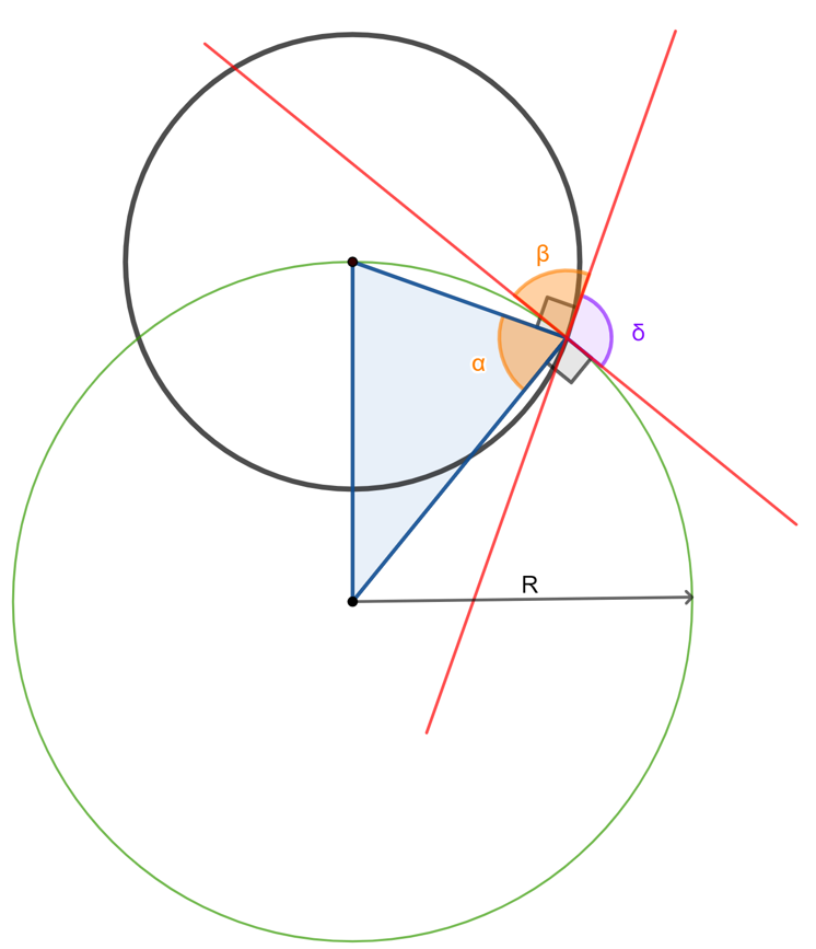
Figure 4: Construction of the proof of Lemma 2.2. We consider the triangle joining the center of the unit disk, the center of the hypercirlce and their point of intersection. Using properties of the tangent lines at the point of intersection, we can relate the radius R to the curvature at (0,0) and $\beta$.

First, notice that $\beta=\alpha$. This is because the radius at the point of tangency is perpendicular to the tangent (red lines). Therefore, we get that $\delta=\pi-\alpha$, which leads to $\delta+\beta=\pi$ and $\beta=\alpha$. Now, let us construct the blue triangle as shown in Figure 4. Using some trigonometric identities we get that

$$\sin\left(\frac{\pi}{2}-\alpha\right)=\frac{1}{2R}.$$

Hence,

$$2\cos(\alpha)=\frac{1}{R}.$$

The hypercircle $\Gamma$ at (0,0) has Euclidean curvature $\frac{1}{R}=2\cos(\alpha)$. Therefore, from Lemma 2.1, the hyperbolic curvature of $\Gamma$ at (0,0) is $\cos(\alpha)=(\cos(\beta))$. Since (0,0) is not a special point, every point of $\gamma$ has hyperbolic curvature $\cos(\beta)$. ∎

Lemma 2.3.

If all points of a hypercircle $\Gamma$ lie at a distance $R>0$ from a certain geodesic, then $\cos(\beta)=\tanh(R)$, where $\beta$ is the angle between $\Gamma$ and the boundary of the model.

Proof.

In the Upper-Half plane model of Hyperbolic space, hypercircles $\Gamma$ with respect to the geodesic line $x=0$ can be represented as straight lines intersecting the boundary with an angle $\beta<\frac{\pi}{2}$. In this model, the distance $R$ between $\Gamma$ and the geodesic is defined by the arc that intersects both lines and meets the boundary perpendicularly, as illustrated in Figure 5.

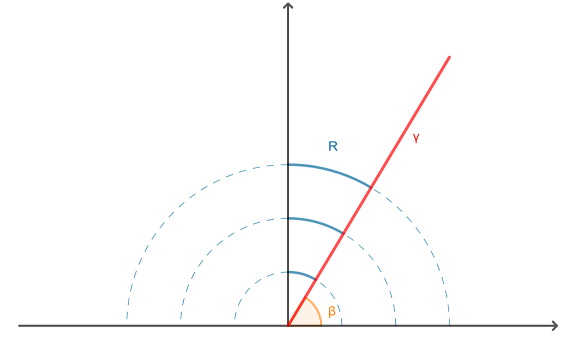
Figure 5: Hypercircle in the Upper Half-Plane

We can parameterize these family of arcs as:

$$\sigma(t)=(A\cos(t),A\sin(t))$$

for $A>0$. Then, $R$ can be obtained by calculating the hyperbolic length of $\sigma(t)$ from $\beta\leq t\leq\frac{\pi}{2}$,

$$R=\int_{\beta}^{\frac{\pi}{2}}\frac{|\sigma^{{}^{\prime}}(t)|}{\text{Im}(\sigma(t))}\text{dt}=\int_{\beta}^{\frac{\pi}{2}}\frac{1}{\sin(t)}\text{dt}=\log(\tan(\frac{\beta}{2})).$$

Then,

$$\tanh(R)=\tanh(\log(\tan(\frac{\beta}{2})))=-\cos(\beta).$$

The negative sign comes from the direction of the normal component. Therefore, $\tanh(R)=|\cos(\beta)|$ as required. Note that when $\Gamma\subset\mathbb{H}^{2}(-c^{2})$ then the curvature $\lambda$ of $\Gamma$ is normalized to $\lambda=c\cdot\tanh(cR)$. ∎

Lemma 2.4.

Let $\Gamma$ be the hypercircle a distance $R$ from the geodesic joining the center of two balls of radius $R$ and curvature $\lambda$. Then, the curvature of the hypercircle is $\frac{1}{\lambda}$.

Proof.

The curvature of a circle of radius $R$ is $\coth(R)$. From Lemma 2.3, the curvature of the hypercircle is $\tanh(R)=\tanh(\coth^{-1}(\lambda))=\frac{1}{\lambda}$, as required.

∎

3 Proof of Theorems A, B and C

The proof of Theorem A is divided into 3 steps. The strategy is as follows:

1. Given a thick $\lambda$-concave body we construct a body $H$ named the Thick Convex Hull of $K$ such that $H\subset K$. We do that by analyzing the structure of the cut locus $T$ of $K$ (subsection 3.1).

2. We then define the inner parallel bodies of both $H$ and $K$ (subsection 3.2).

3. We use the classical Steiner’s formula to relate the area between these two bodies (subsection 3.3) and their inner parallel bodies.

3.1 Construction of the Thick Convex Hull of $K$

The first step is to construct a body $H$ (named the Thick Convex Hull of $K$), such that $H\subset K$. We will do that by analyzing the structure of the cut locus $T$ of $\partial K$. The following definitions are needed for the analysis (see [18]):

Definition 3 (Cut Locus).

Let $K$ be a connected domain with picewise smooth boundary $\partial K$. The cut locus $T$ of $K$ with respect to its boundary $\partial K$ is defined as the closure of the set of all points $x\in K$ such that the restriction of the distance function $d(x,\partial K)$ attains its global minimum at two or more points of $\partial K$ or, in other words, for which there exist two or more points in $\partial K$ minimizing the distance to $x$ [18].

Definition 4 (Focal Point).

Let $K$ be a domain with smooth boundary $\partial K$. For each point $x$ belonging to a cut locus $T$, consider the subset $X\subset\partial K$ where the minimal distance to $x$ is attained. We say that $x$ is a focal point if these equivalent statements are satisfied [18]:

• $X$ is connected

• For any sufficiently small neighborhood $U\ni x$, the complement $U\backslash T$ is connected

If $x\in T$ is not a focal point, then we say that is a cut point.

An illustration of the cut locus and focal points of $\partial K$ for $K\subset\mathbb{H}^{2}$ is shown in Figure 6.

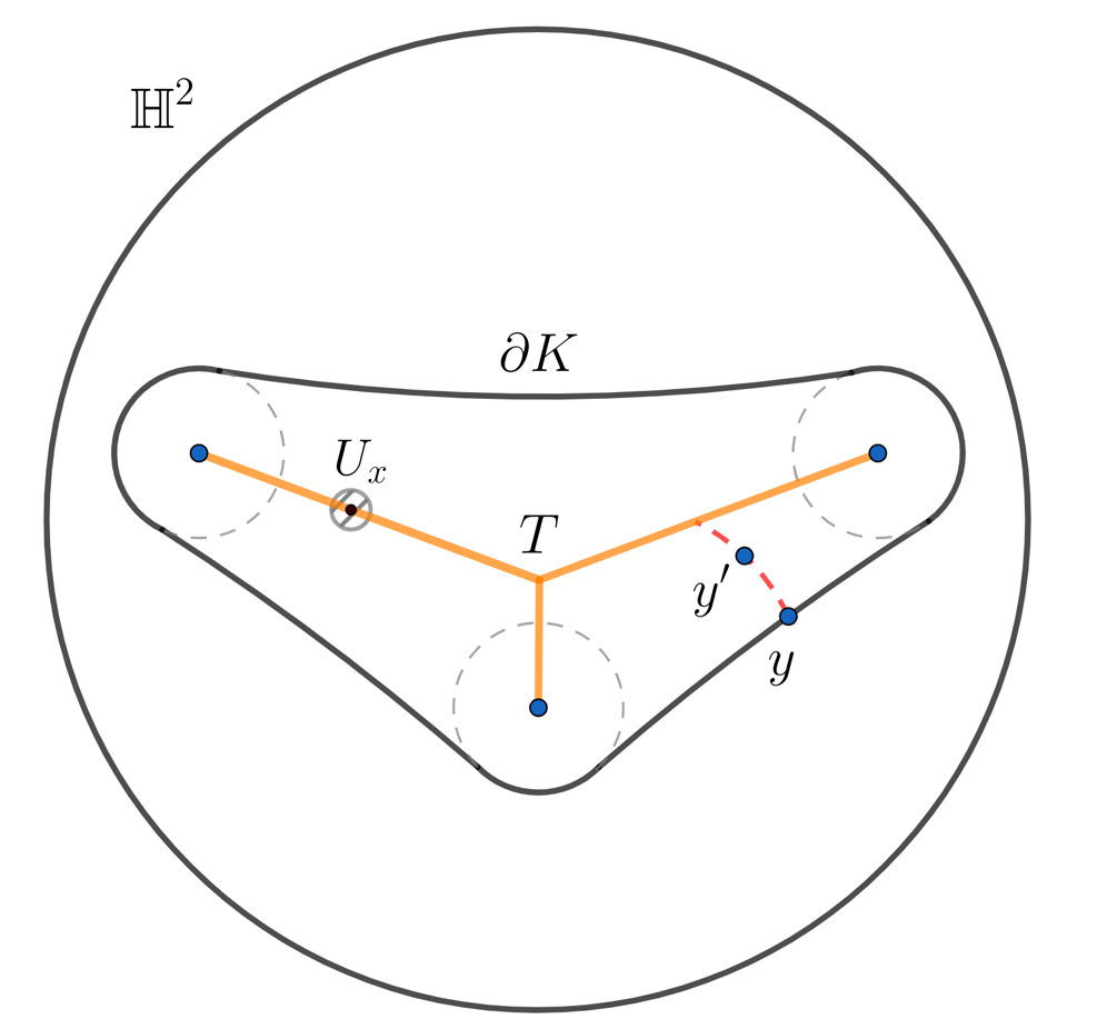
Figure 6: Cut locus of $\partial K$

Definition 5 (Strong Deformation Retract).

A subspace $A$ of a topological space $X$ is a strong deformation retract of $X$ if there is a homotopy $F:X\times I\to X$such that:

$$F(x,0)=x\quad\forall x\in X$$

$$F(a,t)=a\quad\forall a\in A,t\in I$$

$$F(x,1)\in A\quad\forall x\in X$$

Lemma 3.1 (Structure of the cut locus away from focal points [19]).

Let $K\in\mathbb{H}^{2}$ be a convex domain with cut locus $T$ and let $P\in T$ be a cut point that is not a focal point with $R=\text{d}(P,\partial K)$. Then there is a finite number of $k\geq 2$ of minimizing geodesics from $P$ to $\partial K$, and

• Case 1. If $k=2$, then there is a neighborhood $U$ of $P$ so that $T\cap U$ is a $C^{1}$ curve and the tangent to $T$ at $P$ bisects the angle between the two minimizing geodesics from $P$ to $\partial K$.

• Case 2. If $k\geq 3$, then the $k$ geodesic segments from $P$ to $\partial K$ split the disk $B_{R}(P)$ into $k$ sectors $S_{1},\dots,S_{k}$. There is a small open disk $U$ around $P$ so that in each sector $S_{i}$ the set $T\cap U\cap S_{i}$ is a $C^{1}$ curve ending at $P$ and the tangent to this curve at $P$ is the angle bisector of the two sides of the sector $S_{i}$ at $P$ (see Figure 7).

The proof of Lemma 3.1 can be found in [19]. Below there is a diagram showcasing the statement of the Lemma.

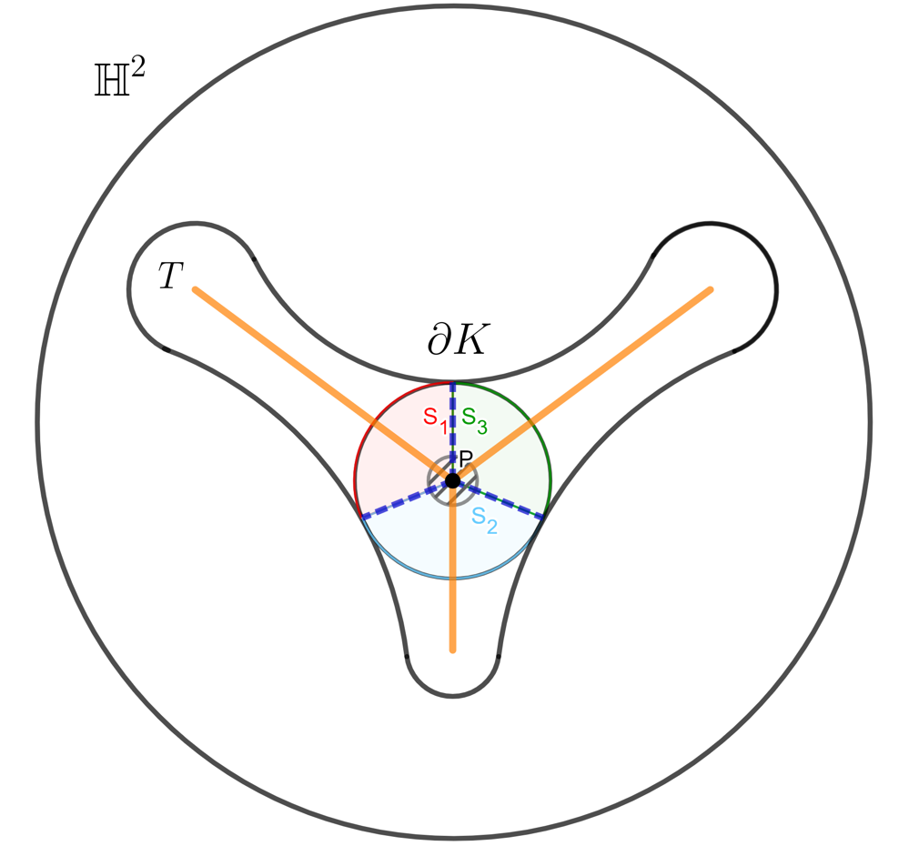
Figure 7: Diagram of Lemma 3.1. The orange line is the cut locus $T$ of $\partial K$ and the slashed blue lines are the 3 geodesics from $P$ to $\partial K$.

Note that from Lemma 3.1, any vertex of $T$ which is not a focal point must be of valance at least 3.

Lemma 3.2.

Let $K$ be a convex body in $\mathbb{H}^{2}$. The cut locus $T$ is a strong deformation retract of $K$ [19].

This retraction can be obtained by considering each point $y^{\prime}\in K\backslash T$ and the corresponding point $y\in\partial K$ that minimizes the distance d($y,y^{\prime}$). We can then move $y$ towards $T$ along the geodesic $[y,y^{\prime}]$. A consequence of Lemma 3.2 is that $K$ and $T$ are homotopy equivalent. In particular, if $K$ is simply connected, then $T$ must also be simply connected and, hence, a tree.

Lemma 3.3.

Let $K$ be a $\lambda$-concave body different from a disk. Then, there exists at least two disks of radius $\coth^{-1}(\lambda)$ contained in $K$.

Proof.

We may assume that $T$ is a tree embedded in $K$ with a finite number of edges. From Lemma 3.1 any vertex of degree 1 must be a focal point. Hence, it contains at least two focal points which corresponds to the leaves of $T$ (except when $K$ is a disk, in which case, it only contains one focal point). In addition, from Definition 4 if $x$ is a focal point, then there exists a $z\in\partial K$ such that the osculating circle at $z$ is centered at $x$. Since $\partial K$ has curvature at most $\lambda$, the radius of the osculating circle is at least $R=1/c\cdot\coth^{-1}(\lambda/c)$. Hence, the distance from $x$ to $\partial K$ is at least $R$, which proves that in each leave of $T$ there is an osculating circle $B_{R}$, of radius $R$, such that $B_{R}\subset K$. ∎

Lemma 3.4.

Let $K\subset\mathbb{H}^{2}$ be $\lambda$-concave body different than a disk. Then,

$$|K|>4\pi\left(\frac{1}{\sqrt{1-\frac{1}{\lambda^{2}}}}-1\right)$$

Proof.

From Lemma 3.3, we have that a $K$ contains at least 2 disks of radius $R=\coth^{-1}(\lambda)$. We can then use the formula for the area of a disk in the hyperbolic space to get the desired inequality. ∎

Definition 6 (Thick Convex Hull of T).

Let $T$ be the cut locus of a thick $\lambda$-concave body $K\subset\mathbb{H}^{2}(-c^{2})$ and let $V(T)$ be the set of vertices of $T$. For all $i\in V(T)$ consider the ball $B_{i}$ centered at the vertex $i$ and with curvature $\lambda_{i}$, where $\lambda_{i}$ is the minimum curvature such that $B_{{}_{i}}\subset K$ (note that $\lambda_{i}\leq\lambda\,\,\forall i$ ). The Thick Convex Hull of $T$ of curvature $\lambda$ is defined as

$$\text{ThickConv }(T,\lambda):=\bigcup_{x,y\in W}[x,y]_{\lambda}$$

where $W$ is the convex hull of $\bigcup B_{i}$ and $[x,y]_{\lambda}$ is the region bounded by two hypercircles of curvature $1/\lambda$ joining $x$ and $y$.

Theorem 1.

(Blaschke Rolling Theorem [20, 13]) If $K\subset\mathbb{H}^{2}$ satisfies $\kappa\geq\ 1/\lambda$ then $\forall x,y\in K$ we have that $[x,y]_{\lambda}\subset K$. ∎

The proof of Theorem 1 can be found in [20]. From this Theorem we get that $\text{ThickConv }(T,\lambda)\subset K$. Figure 8 shows $\text{ThickConv }(T,\lambda)$ (where $\lambda$ is the curvature of the circles centered at the vertices of $T$) and its respective convex hull $W$.

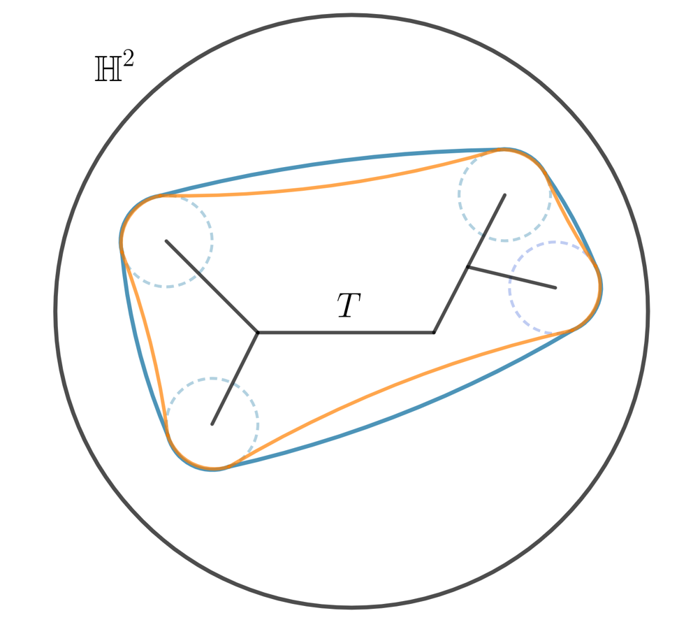
Figure 8: Example of a Thick Convex Hull of $T$ and convex hull (region bounded by blue lines and orange lines, respectively)

Remark: Notice that it is not possible for a ball $B_{\lambda}$ (ball of curvature $\lambda$) centered at vertex of $T$ to be fully contained in the interior of $\text{ThickConv }(T,\lambda)$, like the situation exemplified in the Figure 9 . This is because from Definition 4, if a vertex $v$ is a focal point, there exists a subset $X\subset\partial K$, for $K=\text{ThickConv }(T,\lambda)$, such that the minimal distance to $v$ is achieved for all $x\in X$.

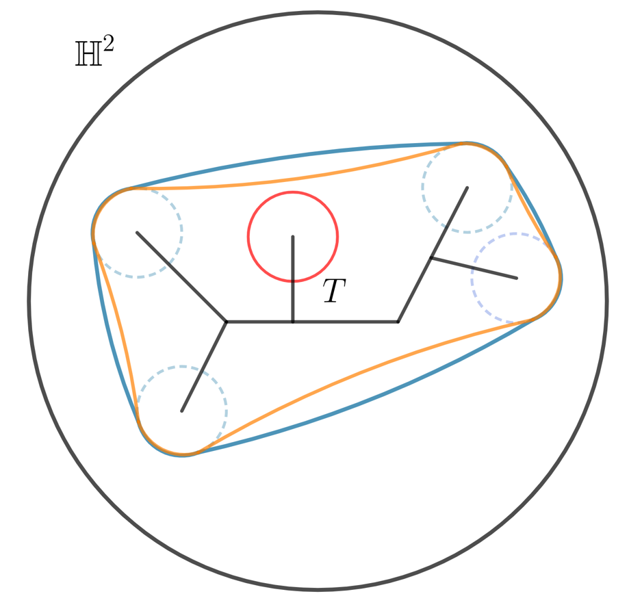
Figure 9: Non-possible construction of the Thick Convex Hull

3.2 Construction of the inner parallel bodies

The next step of the proof constructs the inner parallel bodies of both $K$ and its Thick Convex Hull.

Definition 7 (Inner parallel bodies $K_{-\rho}$ of $K$).

Let $K$ be a convex body in $\mathbb{H}^{2}$. The inner parallel body at distance $\rho\geq 0$ is defined as

$$K_{-\rho}:=\{x\in\mathbb{H}^{2}:B_{\rho}(x)\subset K\},$$

where $B_{\rho}(x)$ is a ball of radius $\rho$ centered at $x$. The greatest number $\rho$ for which $K_{-\rho}$ is not empty is the inradius $in(K)$ of $K$. Equivalently, $in(K)$ is the radius of the largest ball contained in $K$.

Remark: Note that for all $N\in\mathbb{N}$, there exists a strictly convex body body $\Omega\subset\mathbb{H}^{2}$ such that it has $N$ inscribed balls not connected by continuous motion within $\Omega$. We can construct this body $H$ by taking of the convex hull of $N$ equal balls, suitably choosen, and considering the outer parallel body $H_{\epsilon}$ for a small $\epsilon>0$. This ensures that $H_{\epsilon}$ is strictly convex. This phenomena is not encountered in the Euclidean space, where there exist a unique inscribed ball for a strictly convex body $\Omega\subset\mathbb{R}^{2}$.

Remark: Note that $K$ being convex does not guarantee that $K_{-\rho}$ is convex, as shown in Figure 10. In that case, $K$ is the convex hull of two balls $B^{1}$ and $B^{2}$ of radius $R$. The inner parallel body $K_{-\rho}$ for $0<\rho<in(K)$ is the concatenation of the hypercircles a distance $\rho$ from the geodesics with the two balls of radius $r=R-\rho$. It is well known that hypercircles are convex, therefore, there exist a geodesic $[x,y]$ for $x\in B^{1}_{-\rho}$ and $y\in B^{2}_{-\rho}$ such that $[x,y]\nsubseteq K_{-\rho}$ (represented by the orange line in Figure 10 below). This fact is a consequence of the previous remark.

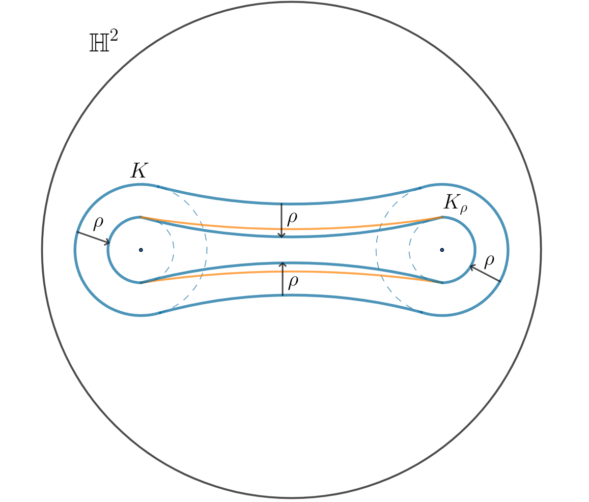
Figure 10: Example of an inner body of a convex body which is not convex

Because of this Remark, is not immediate that the inner parallel body of the Thick Convex Hull of $K$ is convex. We will proceed to prove this is indeed the case with the following lemmas.

Lemma 3.5.

Let $S$ and $K$ be convex subsets of $\mathbb{H}^{2}$. If $S\subset K$, then $S_{-\rho}\subset K_{-\rho}$ for $0\leq\rho\leq in(S)$.

Proof.

Let $x\in S_{-\rho}$. By the definition of inner parallel body $B_{\rho}(x)\subset S\subset K$, which implies that $x\in K_{-\rho}$. This is satisfied $\forall x\in S_{-\rho}$, so we conclude that $S_{-\rho}\subset K_{-\rho}$, as required. ∎

Combining Theorem 1 and Lemma 3.5, we get the following inclusion relationships:

$$\text{ThickConv }(T,\lambda)\subset K$$

$$\left(\text{ThickConv }(T,\lambda)\right)_{-\rho}\subset K_{-\rho}$$

Theorem 2.

Let $K$ be a thick $\lambda$-concave body, let $T$ be the cut locus of $K$ and $H=\text{ThickConv }(T,\lambda)$. Then $H_{-\rho}$ is a convex simply connected domain for $0\leq\rho\leq\coth^{-1}(\lambda)$.

Proof.

We will first prove that $H_{-\rho}$ is simply connected. Let us define an arbitrary ordering of the vertices of $T$ such that

$$\text{ThickConv }(T,\lambda)=W\cup[B_{\lambda}(x_{i}),B_{\lambda}(x_{i+1})]_{\lambda},$$

where $W$ is the convex hull of $\bigcup B_{i}$, as of definition 6, and $[B_{\lambda}(x_{i}),B_{\lambda}(x_{i+1})]_{\lambda}$ is the region bounded by arcs of hypercircle of curvature $1/\lambda$ and two circular arcs of curvature $\lambda$ centered at two consecutive $x_{i}$ and $x_{i+1}$, as shown in Figure 11. Then, by construction $H_{-\rho}$ is simply connected and well-defined for $0\leq\rho\leq 1/c\cdot\coth^{-1}(\lambda/c)$.

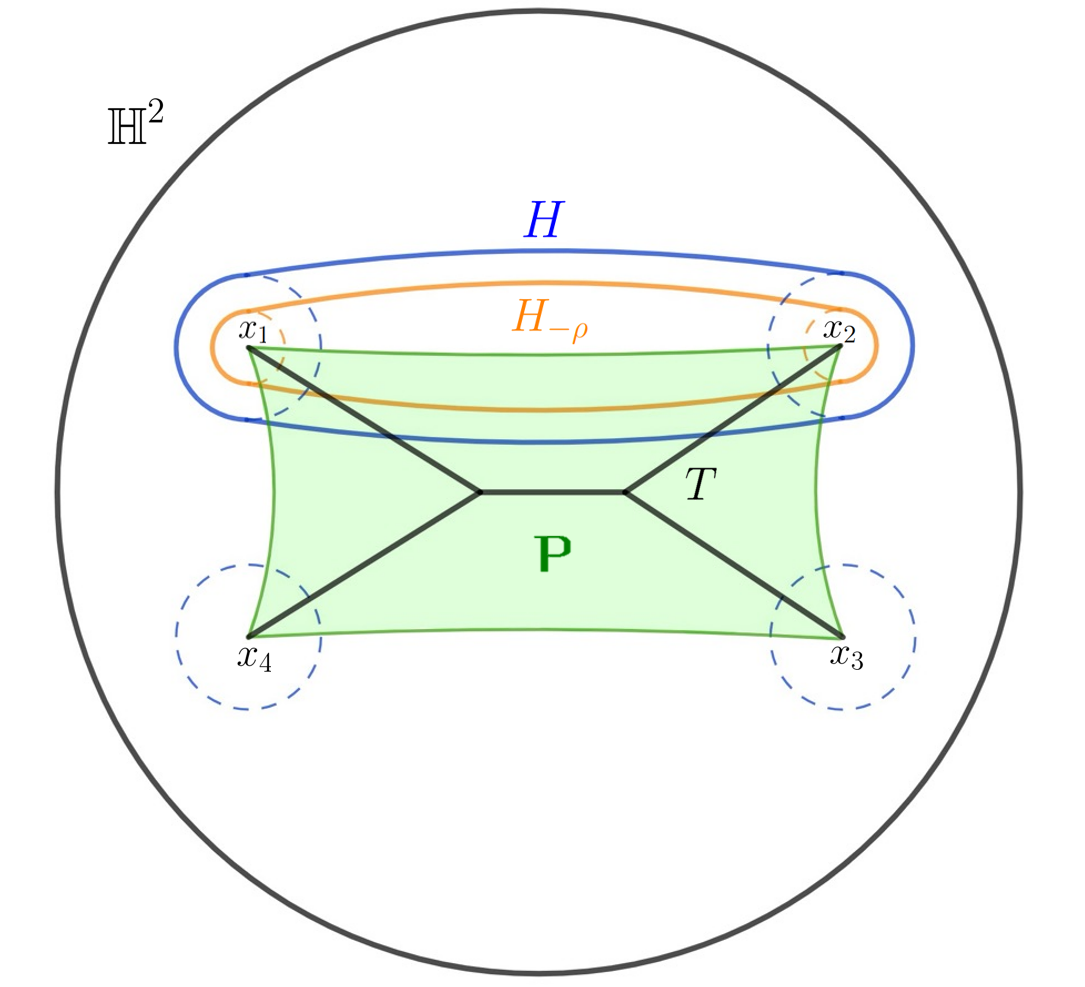
Figure 11: Construction of $H$ and $H_{-\rho}$ from the proof of Theorem 2 for vertices $x_{1}$ and $x_{2}$

Now, if $H_{-\rho}$ is a simply connected domain and $\partial H_{-\rho}$ is $C^{1}-$smooth with $\kappa(x)\geq 0\,\,\forall x\in\partial H_{-\rho}$ (consistent curvature sign in the boundary), then $H_{-\rho}$ is convex (proof of this statement can be found in [21]). ∎

3.3 Steiner’s formula in the Hyperbolic space

We will now use Steiner’s formula to relate the area of a body $K$ with the area of its inner parallel body. According to Steiner’s classical result, if $\partial K$ is an arbitrary convex curve in the plane of length $|\partial K|$ and area $|K|$ and $\partial K_{\rho}$ is a curve parallel to $\partial K$ at a distance $\rho$ with length $|\partial K_{\rho}|$ and area $|K_{\rho}|$. Then,

$$|\partial K_{\rho}|=|\partial K|+2\pi\rho,\quad|K_{\rho}|=|K|+\rho|\partial K|+\pi\rho^{2}$$

We would like to work with a generalization of the Steiner’s formula for the Hyperbolic space. To do that, we have to choose a coordinate system in which $v^{1}=0$ is the curve $\partial K$, and in which $v^{2}=\text{constant}$ are the geodesics orthogonal to $\partial K$, where $\partial K$ is a simple, closed, bounding, and differentiable curve. Further let $v^{2}$ be the arc length of $\partial K$ measured positively for motion on the curve which keeps the bounded area to the left, and let $v^{1}$ be the arc length of geodesics normal to $\partial K$ measured positively outward from $\partial K$. Choose the unit normals to $\partial K$ so that they point toward the interior of $\partial K$. We can now use the following Lemma due to Steiner’s [22]:

Lemma 3.6.

(Steiner’s formula in spaces of negative curvature [22]) Choose $\partial K$ and the coordinate system as above, satisfying

$$\kappa_{g}(v^{2})\sinh(v^{1})+\cosh(v^{1})>0$$ (1)

for $\kappa_{g}(v^{2})>0$ and $\rho\geq 0$. The area of the inner parallel body $A_{\rho}$ with respect to $A$ is then

$$|K_{\rho}|=|\partial K|\sinh\left(\rho\right)-2\pi\left(\cosh\left(\rho\right)-1\right)+|K|\cosh\left(\rho\right).$$ (2)

For our purpose, we want to work with the Steiner inequality when $\rho\leq 0$. Setting $v^{1}=-\rho$ for $\rho\geq 0$, we have that inequality 1 can then be adapted as follows:

$$\kappa_{g}(v^{2})<\coth(\rho)$$ (3)

and formula 2 becomes

$$|K_{-\rho}|=-|\partial K|\sinh\left(\rho\right)-2\pi\left(\cosh\left(\rho\right)-1\right)+|K|\cosh\left(\rho\right)$$

Rearranging, we get that

$$|K|=|K_{-\rho}|\operatorname{sech}(\rho)+|\partial K|\tanh\left(\rho\right)+2\pi\left(1-\operatorname{sech}(\rho)\right).$$ (4)

Note that inequality 3 is included in the assumptions of Theorem A when setting $\kappa<\lambda$.

We will are now ready to finalize the proof of Theorems A and B.

Proof of Theorem A:Let $K\subset\mathbb{H}^{2}$ be a thick $\lambda$-concave body and $S\subset\mathbb{H}^{2}$ be a thick $\lambda$-sausage. For $\rho=\coth^{-1}(\lambda)$, $S_{-\rho}$ is a geodesic with $|S_{-\rho}|=0$. Now, let $T^{\prime}$ be the cut locus of $S$ with $H^{\prime}=\text{ThickConv }(T^{\prime},\lambda)$, and let $T$ be the cut locus of $K$ with $H=\text{ThickConv }(T,\lambda)$. Then, by Theorem 2, $H_{-\rho}\subset K_{-\rho}$ is a simply connected domain, and $0=|S_{-\rho}|=|H^{\prime}_{-\rho}|\leq|H_{-\rho}|\leq|K_{-\rho}|$. Now, if $|\partial S|=|\partial K|$ by Steiner’s result we get that $|S|\leq|K|$ as required.

To proof the other direction, notice that if $|K_{-\rho}|=0$ then $|K_{-\rho}|$ is a convex region with null area and, hence, a geodesic. $K_{-\rho}$ is a a geodesic when $K$ is thick $\lambda$-sausage body, as defined in Definition 6, and $\rho=\coth^{-1}(\lambda)$.

Proof of Theorem B: Substituting $\rho=\coth^{-1}(\lambda)$ in equation (2), we get that the area of the thick $\lambda$-sausage is

$$|K|=\frac{|\partial K|}{\lambda}+2\pi\left(1-\sqrt{1-\frac{1}{\lambda^{2}}}\right).$$ (5)

Applying the appropriate scaling, when $K\subset\mathbb{H}^{2}(-c^{2})$, (5) becomes

$$|K|\geq\frac{|\partial K|}{\lambda}+\frac{2\pi}{c^{2}}\left(1-\sqrt{1-\frac{c^{2}}{\lambda^{2}}}\right).$$

It is easy to check (applying the Hôpital Rule twice) that as $c\rightarrow 0$ from the left, equation 5 approaches the result in the Euclidean space proved in [4].

This concludes the proof of one direction of Theorem B. The other direction is trivial.

Proof of Theorem C: We will prove Theorem C by contradiction. Let $K$ be a thick $\lambda$-concave body and assume a ball $B$ of curvature $\lambda$ can not roll freely in $K$. Then, there exists a ball $B^{\prime}$ of curvature $\lambda^{\prime}>\lambda$ such that $B^{\prime}$ touches $\partial K$ at least twice. Name two of these points of intersection $x$ and $y$. Now, let $z$ be the center of $B^{\prime}$ and consider the geodesic $[x,z]$ and $[y,z]$, as shown in Figure 12. By construction, these geodesics are orthogonal to $\partial K$ so, by Definition 3, $z$ belongs to the cut locus $T$ of $K$. Hence, the distance $\text{d}(T,\partial K)\leq\coth^{-1}(\lambda^{\prime})<\coth^{-1}(\lambda)$. Nevertheless, in Lemma 3.5 we proved that $\text{ThickConv }(T,\lambda)\subset K$ and, hence, d($T,\partial K$) $\geq\coth^{-1}(\lambda)$, arriving at a contradiction.

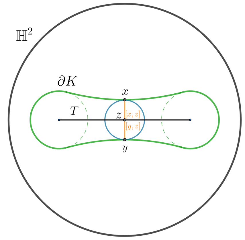
Figure 12: Proof of Theorem C

To prove that the result is false if the curvature is bounded as $1/\lambda^{\prime}\leq k\leq\lambda$ for some $\lambda^{\prime}>\lambda$, consider the convex body $Q$ bounded by two equal circular arcs of curvature $\lambda$ and two equal arcs of hypercircle of curvature $1/\lambda-\epsilon$ for $\epsilon>0$. Then, by construction, a ball of curvature $\lambda$ will not be able to roll freely inside $Q$.

References

- [1] Antonio Ros. The isoperimetric problem. In Global theory of minimal surfaces, volume 2. American Mathematical Society, 2005.
- [2] Keith Ball. Volume ratios and a reverse isoperimetric inequality. J. London Mathematical Society, 44, 1991.
- [3] Kostiantyn Drach and Kateryna Tatarko. Reverse isoperimetric problems under curvature constraints. arXiv:2303.02294v1 [math.MG], 2024.
- [4] Roman Chernov, Kostiantyn Drach, and Kateryna Tatarko. A sausage body is a unique solution for a reverse isoperimetric problem. Advances in Mathematics, 353, 2019.
- [5] Eugenia Saorín Gómez and Jesus Yepes Nicolás. On a reverse isoperimetric inequality for relative outer parallel bodies. Proc. Amer. Math. Soc., 148(11), 2020.
- [6] Piotr Nayar. Reverse isoperimetric inequalities for parallel sets. arXiv preprint arXiv:2102.03680, 2021.
- [7] Aleksander Borisenko and Kostiantyn Drach. Isoperimetric inequality for curves with curvature bounded below. Mathematical Notes, 95(5), 2014.
- [8] Ferenc Fodor, Arpad Kurusa, and Viktor Vígh. Inequalities for hyperconvex sets. Adv. Geom., 16(3), 2016.
- [9] Wilhelm Blaschke. Kreis und Kugel. Chelsea, New York, 1949.
- [10] Jeffrey Rauch. An inclusion theorem for ovaloids with comparable second fundamental forms. Journal of Differential Geometry, 9, 1974.
- [11] Jeffrey Brooks and John Strantzen. Blaschke’s rolling theorem in . Memoirs of the American Mathematical Society, 80(405), 1989.
- [12] Hermann Karcher. Umkreise und inkreise konvexer kurven in der sphärischen und der hyperbolischen geometrie. Mathematische Annalen, 177, 1968.
- [13] Anatoliy Milka. A certain theorem of schur–schmidt. Ukrainian Geometrical Collection, 8, 1970.
- [14] Ralph Howard. Blaschke’s rolling theorem for manifolds with boundary. Manuscripta Mathematica, 99(4), 1999.
- [15] Alexander Borisenko and Kostiantyn Drach. Comparison theorems for support functions of hypersurfaces. Dopovidi Natsional’noi Akademii Nauk Ukrainy, Matematika, Prirodoznavstvo, Tekhnichni Nauky, (3), 2015. arXiv:1402.2691.
- [16] Alexander Borisenko and Kostiantyn Drach. Extreme properties of curves with bounded curvature on a sphere. Journal of Dynamical and Control Systems, 21(3):311–327, 2015.
- [17] Yuriĭ Dmitrievich Burago and Viktor Abramovich Zalgaller. Geometric Inequalities. Springer-Verlag, New York, 1988.
- [18] Anton Petrunin. Puzzles in geometry that i know and love. Association for Mathematical Research, 2, 2022.
- [19] Ralph Howard and Andrejs Treibergs. A reverse isoperimetric inequality, stability and extremal theorems for plane curves with bounded curvature. Rocky Mountain Journal of Mathematics, 25(2), 1995.
- [20] Kostiantyn Drach. The blaschke rolling theorem in riemannian manifolds of bounded curvature. arXiv preprint arXiv:2005.00932, 2024.
- [21] Alfred Gray, Elsa Abbena, and Simon Salamon. Modern Differential Geometry of Curves and Surfaces with Mathematica. CRC Press, 3rd edition, 2006.
- [22] Enrique Vidal Abascal. A generalization of Steiner’s formulae. Bulletin of the American Mathematical Society, 53(8), 1947.