Weak* solutions III: A convergent front tracking scheme

Manas Bhatnagar and Robin Young
Abstract.

We present a variation of the Front Tracking (FT) method for modeling solutions to hyperbolic systems in one space dimension, a Modified FT scheme. Instead of using non-entropic shocks, we approximate simple waves by jumps which exactly match the states, while approximating the wave speed. Our construction makes use of compression curve as well. We work with weak* solutions introduced in [MY17]. Consequently, we are able to analyze residuals rather than errors, and obtain cleaner convergence results. Through this paper, we intend to set up a scheme that is capable of handling strong shocks consistently. We develop this scheme primarily to prove (in a future work) existence of large amplitude solutions of the p-system. Therefore, we treat the p-system more carefully and construct a completely self-sufficient scheme, which has a limit as long as the approximate weak* solutions have uniformly bounded variation. This is a preprint version and will be updated very soon.

Department of Mathematics and Statistics, University of Massachusetts Amherst, mbhatnagar@umass.edu
Department of Mathematics and Statistics, University of Massachusetts Amherst, young@math.umass.edu

1. Front Tracking Approximation

Consider the general $N\times N$ system of hyperbolic conservation laws (in canonical form) in 1D spatial variable,

$\displaystyle u_{t}+f(u)_{x}=0,\quad\mathbb{R}\times(0,T),$ (1)

for any fixed positive constant $T$. Here $u$ takes values in a state space $\Omega\subset\mathbb{R}^{N}$ and $f:\mathbb{R}^{N}\to\mathbb{R}^{N}$ is a $C^{2}$ function, and the strict hyperbolicity condition amounts to the matrix $Df$ having real eigenvalues with an order,

$$\lambda^{1}(u)<\lambda^{2}(u)<\ldots<\lambda^{N}(u),$$

for all $u\in\Omega$. Therefore, there exist $N$ linearly independent eigenvectors, $r^{1}(u),\ldots,r^{N}(u)$, so that,

$$Df(u)r^{i}(u)=\lambda^{i}(u)r^{i}(u),\quad i=1,2,\ldots,N.$$

We normalize eigenvectors to unit vectors, that is, $|r^{i}(u)|=1$. The Cauchy problem is (1) with initial data $u(x,0)=v(x)\in L^{\infty}(\mathbb{R})$. It is generic that the solutions to this Cauchy problem develop discontinuities even if the $v$ is smooth. Hence, we look for solutions in an appropriate space that can accommodate these discontinuities. A locally bounded measurable function $u$ is called a weak solution of (1) if for all test functions $\psi\in C_{c}^{\infty}([0,T)\times\mathbb{R})$ (smooth functions with compact support),

$$\int_{0}^{T}\!\!\!\int_{\mathbb{R}}u\,\psi_{t}+u\,\psi_{x}\,dxdt+\int_{\mathbb{R}}v(x)\psi(x,0)\,dx=0.$$

In [MY17], the authors introduced another notion of solutions, the weak* solutions. In their work, they prove the equivalence of weak* solutions and weak solutions under reasonable growth assumptions. In this paper, we work with weak* solutions and give a different perspective to arrive at the existence of solutions to hyperbolic systems.

We are concerned with physical systems, that is, for which there is an entropy-entropy flux pair $(\eta,q)$, where $\eta,q$ are scalar functions of the state variable $u$. An admissible solution to (1) satisfies the following inequality as distributions,

$$\eta_{t}+q_{x}\leq 0,$$

with equality holding where the solution is $C^{1}$. This inequality denotes the entropy production. Therefore, for admissible solutions, the entropy production is nonpositive. It is widely agreed upon that the apt space to look for solutions to (1) is the space of functions with bounded variation. For a function $g\in L^{1}(\mathbb{R})^{N}$, its variation on a compact set $K$ is defined as,

$$Var_{K}(g)=\left(\sum_{k=1}^{N}\left(\sup_{\mathcal{P}}\sum_{i}|(g(x_{i})-g(x_{i-1}))\cdot e_{k}|\right)^{2}\right)^{1/2},$$

where $\mathcal{P}=\{x_{i}\}_{i}$ is a partition of $K$ and $e_{k}$ is the $k-$unit vector. The outer norm could be any $l_{p}$ norm since all norms are equivalent on a finite dimensional space. If $Var_{K}(v)<\infty$ for any compact set $K$, then $v$ is said to be in $BV_{loc}(\mathbb{R})^{N}$. From here onwards, we denote this space as just $BV^{N}_{loc}$. Henceforth, we assume

$\displaystyle v\in BV^{N}_{loc},$ (2)

and we set $v$ to be right continuous. Since functions of bounded variation have countably many discontinuities, the entropy production condition only needs to checked at discontinuities. For a weak solution of (1) with $u(\cdot,t)\in BV_{loc}$ in a time interval, the entropy production inequality can equivalently be checked only on the set of discontinuities. On a discontinuity, the inequality reduces to,

$\displaystyle-\sigma\left(\eta(u^{+})-\eta(u^{-})\right)+\left(q(u^{+})-q(u^{-})\right)\leq 0,$ (3)

where $u^{+},u^{-}$ are states on the right, left of the discontinuity respectively.

The well-posedness of the Cauchy problem, (1),(2) is of great interest to the mathematics as well as physics community. For ‘small’ data, this has been answered to a definitive extent, see [JG65,Yo93,CKV22]. For (1), front tracking schemes/algorithms are a well-known method to obtain approximate solutions, for which if one can obtain bounds, would lead to existence of solution through appropriate compactness argument. A front tracking algorithm provides a piecewise constant approximation to the solution, where shocks are treated exactly and rarefactions are usually approximated by small non-entropic jump discontinuites. Errors in weak solutions are then handled by the use of non-physical waves which decrease with the grid size. Such schemes were first introduced in [RD76]. Several other forms of the scheme exist, see for example [Brbook]. If the initial data is approximated by a piecewise constant function, the solution can be resolved into many Riemann problems. Each Riemann solution consists of shock waves, centered rarefactions, and possibly contact discontinuities; if the solution contains only shocks and contacts, it remains in the class of piecewise constant functions of $x$ for each fixed positive time. To preserve this nice property, we approximate each rarefaction by a series of small jumps emanating from the center of the rarefaction. The usual FT scheme uses several non-entropic rarefaction shocks to approximate the rarefaction. Instead, in our scheme, we use jumps where the adjacent states are exact and therefore, lie on the corresponding simple wave curve. Moreover, we split rarefactions along the evolution whenever a rarefaction reaches a threshold width.

In this paper, we describe a modified front tracking algorithm capable of handling waves of arbitrary strength. Although we give the framework of a general scheme, our primary motive here is to setup a scheme for the $2\times 2$ system of isentropic gas dynamics, to (in a subsequent work) prove existence of large amplitude solutions. A key difference from existing front tracking schemes is that we use compressions, along with rarefactions and shocks, in the scheme. It seems that to obtain large BV existence, one must construct the approximate solution more precisely and use exact states. Owing to the presence of strong shocks, the error in state from the shock curve to the compression curve is $O(1)$, which cannot be controlled globally. Hence, it seems that the usage of compressions is imposed, if one were to analyze large amplitude initial data. Consequently, we need to introduce a new scheme that has this property.

First, we review some properties of solutions to (1). Recall that simple waves, which include both rarefactions and compressions, are integrals of eigenvectors, so they lie on the wave curves $\mathcal{W}^{i}$, which are given by

$$\mathcal{W}^{i}(u_{0})=\Big{\{}u(z):u(z)=W^{i}(z;u_{0}):=u_{0}+\int_{0}^{z}r^{i}(u(\zeta))\;d\zeta\Big{\}},$$ (4)

where $r^{i}(u)$ is the $i$-th eigenvector of $Df(u)$. We consider systems in which all the characteristic families are either genuinely nonlinear or linearly degenerate,

$$\nabla\lambda^{i}\cdot r^{i}>0,\quad\text{OR}\quad\nabla\lambda^{i}\cdot r^{i}=0.$$

The curves $\mathcal{W}^{i}(u_{0})$ describe the states in an $i$-simple wave, while the actual profile of the wave is given by that of the parameter $z=z(x,t)$, which in turn solves the scalar equation

$$z_{t}+\lambda^{i}\big{(}u(z)\big{)}\;z_{x}=0.$$

We solve this equation by characteristics,

$$\frac{dz}{dt}=0\quad\text{on}\quad\frac{dx}{dt}=\lambda^{i}\big{(}u(z)\big{)},$$

so that $z(x,t)=z_{0}=z(x_{0},t_{0})$, for characteristic

$$x=x_{0}+\lambda^{i}\big{(}u(z_{0})\big{)}\,\big{(}t-t_{0}\big{)}.$$ (5)

This solution is valid on the largest neighborhood of a non-characteristic Cauchy curve

$$\Gamma=\Big{\{}\big{(}x_{0}(\gamma),t_{0}(\gamma)\big{)}\Big{\}}$$

for which the characteristic (5) has a unique solution $\gamma(x,t)$. If the characteristic curve $\Gamma$ degenerates to a single point, then the simple wave is centered.

In building our front tracking scheme, we note that the simple wave curve $\mathcal{W}^{i}(U_{0})$ is the solution of the autonomous equation $\frac{dU}{dz}=r^{i}(u)$, so has the group property

$$W^{i}(z_{1}+z_{2};u_{0})=W^{i}\big{(}z_{2};W^{i}(z_{1};u_{0})\big{)},$$ (6)

and in particular,

$$\mathcal{W}^{i}(u_{1})=\mathcal{W}^{i}(u_{0})\quad\text{whenever}\quad u_{1}\in\mathcal{W}^{i}(u_{0}).$$

This means that if we respect the curves $\mathcal{W}^{i}$ when approximating simple waves, the error is essentially in the profile only, while the actual states can be accounted for exactly. Moreover, the derivative $\frac{du}{dz}=r^{i}(u)$ remains uniformly bounded on the open set on which the system remains hyperbolic, so that the wave curves $\mathcal{W}^{i}(u_{0})$ are globally defined: that is, they can be defined up to the boundary of the domain of hyperbolicity.

The usual building block of approximations to conservation laws in one space dimension is the Riemann problem, which is solved using shocks and centered rarefactions. However, the class of simple waves is much larger than that of centered rarefactions, and we wish to exploit these to develop our modified front tracking method. Note that in our notation, contact discontinuities corresponding to a linearly degenerate field can be regarded as (centered) simple waves.

Recall that the $i$-th shock curve $\mathcal{S}^{i}(u_{0})$ through a state $u_{0}$ is the $i$-th solution of the Rankine-Hugoniot condition, namely

$$\sigma\,\big{[}u\big{]}=\big{[}f(u)\big{]},\quad\text{or}\quad\sigma\,\big{(}u-u_{0}\big{)}=f(u)-f(u_{0}).$$ (7)

This is an eigenvalue problem for the matrix

$$\overline{Df}:=\int_{-\frac{1}{2}}^{\frac{1}{2}}Df\big{(}\overline{u}+\eta\,[u]\big{)}\;d\eta,\quad\overline{u}=\frac{u+u_{0}}{2},$$

and solutions are characterized by the shock speed $\sigma$, which are eigenvalues of $\overline{Df}$. For a genuinely nonlinear wave family, an $i$-shock satisfies Lax’s entropy inequality,

$$\lambda^{i}(u_{0})>\sigma>\lambda^{i}(u),$$

and the $i$-th shock curve $\mathcal{S}^{i}(u_{0})$ consists of the right states that can be connected to left state $u_{0}$ by an $i$-shock. If the $i$-th family is linearly degenerate, the curves $\mathcal{W}^{i}(u_{0})$ and $\mathcal{S}^{i}(u_{0})$ coincide, and we will usually treat jumps as (degenerate) shocks.

Since the simple wave curves $\mathcal{W}^{i}(u)$ differ from the shock curves $\mathcal{S}^{i}(u)$, the use of many small rarefaction (non-entropic) shocks to model rarefactions has the advantage of ensuring that the approximations are weak solutions away from nonphysical waves, but with the disadvantage that each time a rarefaction shock is used, an error in the state is introduced, which must be accounted for, say by the use of nonphysical waves.

For us it is more convenient to use the exact wave curve (4) when approximating simple waves, so that we do not introduce state errors, but on the other hand these discontinuities generally fail the jump conditions. This means that our approximations are generally not weak solutions. However, we will be working with weak* solutions, which satisfy the equation as an ODE (upto a residual term) in the space $X^{*}$, which is a dual of some suitable space $X$. In this context, it is easy to calculate the residual of our approximation as a function in $X^{\ast}$, and convergence to a weak* solution follows as long as we show that the residual converges to zero in the limit of mesh parameters.

Now, we review the concept of weak* solutions introduced in [MY17] and define the spaces which we work in. For $1<p\leq\infty$ and a separable Banach space $X$, if $g\in L^{p}(0,T;X^{*})$, then $g:[0,T]\to X^{\ast}$ with,

$$\int_{0}^{T}||g||_{X^{*}}^{p}(t)\,dt<\infty.$$

Let $g^{\prime}$ be the Gelfand-weak derivative (if it exists) of $g$. If $g,g^{\prime}\in L^{p}(0,T;X^{*})$, then $g\in W^{1,p}(0,T;X^{*})$. It is known that for a separable Banach space $X$, and for $1\leq q<\infty$,

$\displaystyle L^{q}(0,T;X)^{*}=L^{p}(0,T;X^{\ast}),$ (8)

where $\frac{1}{p}+\frac{1}{q}=1$. Throughout the paper, we will assume $X=C(K)$, the space of continuous functions on a compact set $K\subset\mathbb{R}$. By Riesz-Markov-Kakutani Theorem, we know that $C(K)^{*}$ is the space of all Radon (signed) measures on $K$, denoted by $\mathcal{M}(K)$. By (8) above, we have in particular,

$\displaystyle L^{1}(0,T;C(K))^{*}=L^{\infty}(0,T;\mathcal{M}(K)).$ (9)

In what will follow, we will drop the explicit dependence of notations on the set $K$ and write the space of measures as $\mathcal{M}_{loc}$, which is the Radon measures. Also, for $p\in[1,\infty]$, let $W^{1,p}(0,T;BV_{loc},\mathcal{M}_{loc})$ be the space of all functions that are in $W^{1,p}(0,T;\mathcal{M}_{loc})$ and for any fixed $t\in[0,T]$, take values in $BV_{loc}$. Also, since we are working with systems, we will refer to $BV_{loc}^{N}$ (or $\mathcal{M}_{loc}^{N}$), that is vectors whose components are functions (or measures) that lie in the mentioned space. Moreover, we will use the Euclidean norm. It can be shown (see for example [MY17]) that for any Banach space $X$,

$$I:(X^{\ast})^{N}\to(X^{N})^{*},$$

given by $[I(G)](x)=\sum_{i=1}^{N}G_{i}(x_{i})$, is an isometric isomorphism. Consequently, for any $\boldsymbol{\mu}\in\mathcal{M}_{loc}^{N}$ , $||\boldsymbol{\mu}||_{\mathcal{M}_{loc}^{N}}=\left(\sum_{i=1}^{N}||\mu_{i}||_{\mathcal{M}_{loc}}^{2}\right)^{1/2}$. From here onwards, we might denote $||\cdot||$ for any norm, on $C,C^{N},\mathcal{M}_{loc},\mathcal{M}_{loc}^{N}$, as long as the context makes it clear as to which space is being referred to.

Definition 1.1.

$\mathbf{u}\in W^{1,\infty}(0,T;BV^{N}_{loc},\mathcal{M}^{N}_{loc})$ is a BV-weak* solution to (1) if

$$u^{\prime}+\mathbb{D}_{x}f(u)=0,\quad\text{in }\mathcal{M}_{loc}^{N},\quad a.e.\,t\in[0,T],$$

or equivalently,

$$\bar{u}(\cdot,t)-\bar{u}(\cdot,0)+*\int_{0}^{t}\mathbb{D}_{x}f(u(\cdot,\tau))\,d\tau\quad\text{in }\mathcal{M}_{loc}^{N},\quad t\in[0,T],$$

where ${}^{\prime},*\!\!\int,\mathbb{D}_{x}$ are the Gelfand weak (time) derivative, Gelfand integral, distributional (space) derivative respectively and $\bar{u}(\cdot,0)$ matches the BV initial data.

$\bar{u}$ represents the absolutely continuous (as a function of time into $\mathcal{M}_{loc}^{N}$) representative of $u$. We know that it exists, see [MY17] for calculations. Also, since $f$ is $C^{2}$, the distributional derivative (in $x$) of $f(u(x,t))$ is a measure for any $t$ as long as $u(\cdot,t)\in BV_{loc}$. Hence, all of the above is well-defined. In the same work, the authors proved that a BV-weak* solution is also a weak solution. We state the result here.

Theorem 1.2.

[[MY17], Theorem 4.3] Suppose $u\in W^{1,\infty}(0,T;BV_{loc},\mathcal{M}_{loc})$ is a BV-weak* solution to the Cauchy problem (1), with continuous representative $\bar{u}$. Then $\bar{u}$ is Lipschitz continuous as a function into $L^{1}_{loc}(\mathbb{R};\mathbb{R}^{N})$. The function $\bar{u}(x,t)$ is a weak solution of the Cauchy problem (1).

Remark 1.3.

By treating the solution space as a dual space, the topology on this space is actually induced by test functions. Hence, we can change test functions and, in turn, change the solution space. For example, when the space of test functions is $H^{-s}$ ($s>3/2$), then we are looking at classical solutions, whereas if $s<1/2$ then we are looking at weak solutions that include BV solutions as well. This point is rather important since this kind of setup allows for us to consider $L^{2}$-based spaces which as proven in [Ra86] are the only hope for well-posedness in multidimension. Moreover, since our setup is quite abstract and does not have much to do with the dimension of the spatial variable but with the space of test functions, we can formally write the definition of weak* solution in multidimension as well. This seems a good way forward to tackle multidimensional spatial variable. The weak* solution in multidimensional spatial variable would a topic of further research.

Through our scheme, we will obtain a family of approximate solutions that all lie in the desired space. As mentioned earlier, our aim is to prove uniform BV bounds on these approximate solutions for the isentropic gas dynamics (or the p-system), by constructing a nonlocal functional. Hence, our main focus will be on the p-system.

1.1. The Riemann Problem

We begin by describing our approximation of a Riemann solution. Recall that an exact Riemann solution consists of $N$ waves, arranged from left to right in increasing order of wavespeed, and each of which consists of a Lax shock, contact discontinuity (if the family is linearly degenerate), or centered rarefaction wave. If the Riemann data consists of the pair $(u_{L},u_{R})$ on the left and right, respectively, then we set $U^{0}=u_{L}$ and denote the state on the right of the $i$-th wave by $U^{i}$. We then have

$$U^{i}\in\begin{cases}\mathcal{S}^{i}(U^{i-1})&\quad\text{if}\quad\lambda^{i}(U^{i-1})>\lambda^{i}(U^{i}),\\ \mathcal{W}^{i}(U^{i-1})&\quad\text{if}\quad\lambda^{i}(U^{i-1})\leq\lambda^{i}(U^{i}),\end{cases}$$

and there is a unique set of states $\{U^{i}\}$ such that $U^{N}=u_{R}$. Existence and uniqueness of solutions of the Riemann problem is an assumption here, because we are considering large data, so that $u_{L}$ and $u_{R}$ need not be close to one another.

Since we want our approximation to be piecewise constant, we use the exact wave if this is a shock or contact, and we simply need to describe the approximation of a single centered rarefaction wave. As usual, we use the convention that $\frac{d\lambda^{i}}{dz}=r^{i}\cdot\nabla\lambda^{i}>0$ along $\mathcal{W}^{i}$. We introduce a small discretization parameter $\epsilon>0$, which would essentially control the strength of the approximate simple wave jumps. This parameter would tend to zero to obtain a weak* solution as the limit.

Thus suppose we are given states $U^{i-1}$ and $U^{i}$, such that

$$U^{i}\in\mathcal{W}^{i}(U^{i-1}),\quad\text{say}\quad U^{i}=W^{i}(Z;U^{i-1});$$

we refer to $Z>0$ as the wave strength. Due to the group property (6), we can treat the single rarefaction wave of strength $Z$ as many smaller adjacent rarefactions of smaller strength. Thus, if we choose $m$ strengths $z_{k}\in(0,\epsilon)$ satisfying $\sum z_{k}=Z$, and inductively define

$$\nu_{0}=U^{i-1}\quad\text{and}\quad\nu_{k}=W^{i}(z_{k},\nu_{k-1}),\quad\text{so that}\quad\nu_{m}=U^{i}.$$

In this way the single large rarefaction of strength $Z$ has been split up into $m$ adjacent small rarefactions of size $z_{k}<\epsilon$, with no error in the states. Indeed, we still have the same exact solution of the Riemann problem, albeit with many waves rather than a single wave in each family.

We now approximate each of these small rarefactions by a single jump discontinuity. Thus the jump between $\nu_{k-1}$ and $\nu_{k}$, which has strength $z_{k}\leq\epsilon$, is given wavespeed $\lambda^{i}_{k}$. As long as the wavespeeds $\lambda^{i}_{k}$ are monotone increasing, the approximation can be consistently defined and we have a piecewise constant approximation of the rarefaction wave. For a genuinely nonlinear family, imposing the condition $\lambda^{i}(\nu_{k-1})<\lambda^{i}_{k}<\lambda^{i}(\nu_{k})$, guarantees monotonicity. By carrying out the same discretization for each rarefaction, we get a (globally defined) piecewise constant approximation of the Riemann solution.

It remains to choose the speed of the various jumps. To do so, we first compute the residual $u_{t}+f(u)_{x}$ of the approximate solution by calculating this as a measure. The residual would vanish identically on a weak* solution, so we wish to choose the wavespeeds in such a way that we control this residual and it vanishes in the limit of discretization parameters.

We can describe the approximation of the jump between states $\nu_{k-1}$ and $\nu_{k}$, having speed $\lambda^{i}_{k}$, as

$$\widehat{u}:=\nu_{k-1}+[\nu]\,H\big{(}x-\lambda^{i}_{k}\,t\big{)},\quad\text{where}\quad[\nu]=\nu_{k}-\nu_{k-1},$$

where $H$ is the (right-continuous) Heaviside function, and so also

$$f(\widehat{u})=f(\nu_{k-1})+[f]\,H\big{(}x-\lambda^{i}_{k}\,t\big{)},\quad\text{where}\quad[f]=f(\nu_{k})-f(\nu_{k-1}).$$

As in [MY17], we can simply differentiate to obtain the residual of this single jump:

$$R\widehat{u}:=\widehat{u}^{\prime}+\mathbb{D}_{x}f(\widehat{u})=-\lambda^{i}_{k}\,[\nu]\,\delta_{\lambda^{i}_{k}t}+[f]\,\delta_{\lambda^{i}_{k}t},$$ (10)

which is interpreted as a time-dependent measure on $\mathbb{R}$, and $\mathbb{D}_{x}$ being the Gelfand weak (time) and distributional (space) derivatives, respectively.

In addition, since all waves in this approximation are centered at the origin and non-overlapping, we can describe the full approximation of the Riemann solution as the sum of all such terms, one for each wave or jump,

$\displaystyle\widehat{U}=u_{L}+\sum_{i,k}[\nu^{i}_{k}]\,H\big{(}x-\lambda^{i}_{k}\,t\big{)},$ (11)

where $k$ ($1\leq k\leq k_{i}$) enumerates the small $i$-jumps if the $i$-wave is simple. Again, summing similar terms yields the residual of the full approximation with many waves,

$$R\widehat{U}=\sum_{i,k}R^{i}_{k}\,\delta_{\lambda^{i}_{k}t}\quad\text{where}\quad R^{i}_{k}:=[f^{i}_{k}]-\lambda^{i}_{k}\,[\nu^{i}_{k}].$$

We note that if the $i$-wave is a shock or contact, then $k_{i}=1,[\nu_{1}^{i}]=U^{i}-U^{i-1}$ and the Rankine-Hugoniot conditions are satisfied, and so provided the correct wavespeed is used, there is no contribution to the residual. This is expected as those jumps are exact.

Using the triangle inequality and the fact that a Dirac mass has norm 1 (as measure), the size of the residual, in the space of measures,

$$\|R\widehat{U}\|(t)\leq\sum_{i,k}\big{|}R^{i}_{k}\big{|}=\sum_{i,k}\Big{|}[f^{i}_{k}]-\lambda^{i}_{k}\,[\nu^{i}_{k}]\Big{|},$$

where $|\cdot|$ denotes the Euclidean norm on $\mathbb{R}^{N}$. Our choice of jump speed $\lambda^{i}_{k}$ is to to minimize the length of the vector $[f]-\lambda^{i}_{k}[\nu]$. Using least squares, we see that this is minimized precisely when $[f]-\lambda^{i}_{k}[\nu]$ is orthogonal to $[\nu]$, so that

$$\lambda^{i}_{k}=\frac{[f]\cdot[\nu]}{\big{|}[\nu]\big{|}^{2}},\quad\text{and}\quad R^{i}_{k}=[f]-\frac{[f]\cdot[\nu]}{\big{|}[\nu]\big{|}^{2}}\,[\nu],$$ (12)

which is the projection of $[f]$ orthogonal to the (unit) direction $[\nu]/|[\nu]|$.

If the wave is a shock or contact, which satisfies (7) exactly, then the contribution to the residual is

$$\big{|}R^{i}_{1}\big{|}=\big{|}\sigma-\lambda^{i}_{1}\big{|}\,\big{|}[u]\big{|}=0.$$ (13)

On the other hand, if the jump is approximating a simple wave, the size of the jump can be assumed small. Since along the $i$-th simple wave curve $\mathcal{W}^{i}$ we have $\frac{du}{dz}=r^{i}$, we write

$$[\nu]=\int_{0}^{z_{k}}r^{i}(u(z))\;dz,\quad\text{and}\quad[f]=\int_{0}^{z_{k}}\lambda^{i}(u(z))\,r^{i}(u(z))\;dz,$$

so that

$$R^{i}_{k}=\int_{0}^{z_{k}}(\lambda^{i}(u(z))-\lambda^{i}_{k})\,r^{i}(u(z))\;dz,$$

and the contribution to the residual is

$\displaystyle\big{|}R^{i}_{k}\big{|}$ $\displaystyle\leq\;\int_{0}^{z_{k}}\big{|}\lambda^{i}(u(z))-\lambda^{i}_{k}\big{|}\;dz$
$\displaystyle\leq O(1)\;\int_{0}^{z_{k}}|z-\bar{z}|\;dz\leq O(1)\,z_{k}^{2},$

provided $\lambda^{i}_{k}$ is chosen to take on some value between $\lambda^{i}(\nu_{k-1})$ and $\lambda^{i}(\nu_{k})$. We regard $\lambda^{i}_{k}$ as a weighted average of $\lambda^{i}(u)$ on the small arc of the wave curve between the states $\nu_{k-1}$ and $\nu_{k}$. The total contribution of the small jumps approximating the simple wave is then

$$\sum_{k}\big{|}R^{i}_{k}\big{|}\leq O(1)\,\max|z_{k}|\,\sum|z_{k}|\leq O(1)\,\epsilon\,|Z|,$$ (14)

where we recall $Z=\sum z_{k}$ is the splitting of the single large simple rarefaction $i$-wave.

Combining expressions (13) and (14), we thus obtain the total residual of our approximation to the Riemann problem, namely

$$\|R\widehat{U}\|(t)\leq O(1)\,\epsilon\,\sum_{i}|Z^{i}|\to 0\quad\text{as}\quad\epsilon\to 0.$$ (15)

It follows that, provided the approximations converge, and the total variation of waves $\sum|Z^{i}|$ is bounded, the limit is a weak* solution of (1). The same bounds and convergence apply for our more general FT approximations, provided the total variation of jumps at time $t$ is bounded. Note that in (15), any positive power of $\epsilon$ on the right-hand-side will serve the purpose. In particular, if

$$\|R\widehat{U}\|(t)\leq O(1)\,\epsilon^{\theta}\,\sum_{i}|Z^{i}|,$$

for some $\theta>0$ will also lead to the same conclusion since $\|R(t)\|$ will still tend to zero as $\epsilon\to 0^{+}$, as long as the variation is bounded. This observation will be useful later.

To fix further notation, we denote the FT approximate solutions we construct in the following form,

$\displaystyle\widehat{U}^{\epsilon}(x,t)=\nu_{0}+\sum_{j}[\nu^{\epsilon}]_{j}\,H\big{(}x-x^{\epsilon}_{j}-\sigma_{j}\,(t-t^{\epsilon}_{j})\big{)},$ (16)

at a particular $t\in[0,T]$, in between interactions. Similar to earlier notation, $[\nu^{\epsilon}]_{j}=\nu^{\epsilon}_{j}-\nu^{\epsilon}_{j-1}$. The states $\nu^{\epsilon}_{j}$’s and the summation index upper limit as well as $x^{\epsilon}_{j},t^{\epsilon}_{j}$’s may be different for different times, owing to interactions. The speed of propagating discontinuities is denoted by $\sigma_{j}$. Note that from now onwards, we treat each wave as an independent one with its own index $j$ as opposed to (11), which has index $i$ for the family and $k$ for each smaller component within the family. Each interaction is solved to emanate new waves and the solution evolves further. Suppose there is a uniform bound on the (absolute) sum of wave strengths in terms of the initial total variation, that is for all $t\in[0,T]$,

$\displaystyle\sum_{j}\left|[\nu^{\epsilon}]_{j}\right|\leq K\ \text{Var}(v).$ (17)

Consequently, note that from (17),

$\displaystyle\sup_{\begin{subarray}{c}t\in[0,T]\end{subarray}}||\widehat{U}^{\epsilon}||_{\mathcal{M}_{loc}}(t)$ $\displaystyle=\sup_{\begin{subarray}{c}t\in[0,T]\end{subarray}}||\widehat{U}^{\epsilon}||_{L^{1}_{loc}}(t)$
$\displaystyle\leq K(|\nu_{0}|+\text{Var}(v)),$

where $K$ is a constant depending on the size of the compact subset under consideration. Also, let $\tau<t$ be two times in between interactions (all times where the delta functions are mutually disjoint), from (17),

$\displaystyle||\widehat{U}^{\epsilon}(\cdot,t)-\widehat{U}^{\epsilon}(\cdot,\tau)||_{\mathcal{M}_{loc}}$ $\displaystyle=\sum_{j}|[\nu^{\epsilon}]_{j}|\int_{|\sigma_{j}|\tau}^{|\sigma_{j}|t}\,ds$
$\displaystyle=\sum_{j}|\sigma_{j}[\nu^{\epsilon}]_{j}|(t-\tau)$
$\displaystyle\leq K\,\text{Var}(v)(t-\tau).$

To get the last inequality, we assumed that $\widehat{U}^{\epsilon}$ has values within a compact set. Consequently, $\widehat{U}^{\epsilon}(\cdot,t)$ is Lipschitz continuous in between interactions. Furthermore, around any time of interaction, $\widehat{U}^{\epsilon}$ is Lipschitz continuous as well. To see this, let us consider a single interaction and the resolution of the Riemann Problem as in the beginning of this section. We can translate a single interaction from any coordinate to occur at the origin to simplify our calculations. So, in an interval around $t=0$, let

$$\widehat{U}^{\epsilon}(x,t)=\left\{\begin{array}[]{lr}(u_{m}-u_{l})H(x-\sigma_{1}t)+(u_{r}-u_{m})H(x-\sigma_{2}t)+E,&t<0,\\ \sum_{i=1}^{N}(U^{i}-U^{i-1})H(x-\lambda^{i}t)+E,&t>0.\end{array}\right.$$

Here, $E=E(x,t)$ is the sum of all other Heavisides that correspond to waves not involved in the interaction. Also, $\sigma_{1}>\sigma_{2}$ and we follow the notation used in the discussion at the beginning of the section, when referring to the resolution of a Riemann Problem. We will take difference of each branch separately with $\widehat{U}^{\epsilon}(x,0)=(u_{r}-u_{l})H(x)+E$. Let’s see for the $t<0$ branch,

$\displaystyle\left\|\widehat{U}^{\epsilon}(x,0)-\widehat{U}^{\epsilon}(x,t)\right\|$
$\displaystyle=$ $\displaystyle\left\|(u_{r}-u_{l})H(x)+E(x,0)-\widehat{U}^{\epsilon}(x,t)-E(x,t)\right\|_{\mathcal{M}_{loc}}$
$\displaystyle=$ $\displaystyle\left\|(u_{m}-u_{l})\left(H(x)-H(x-\sigma_{1}t)\right)+(u_{r}-u_{m})\left(H(x)-H(x-\sigma_{2}t)\right)\right\|$
$\displaystyle\qquad\qquad\qquad\qquad+\left\|E(x,0)-E(x,t)\right\|.$

Note that,

$$\left\|E(x,0)-E(x,t)\right\|=\sum_{j}|\sigma_{j}[\nu]_{j}||t|,$$

where the sum is over all other waves not involved in this interaction. Using this in the difference above, we obtain that,

$\displaystyle\left\|\widehat{U}^{\epsilon}(x,0)-\widehat{U}^{\epsilon}(x,t)\right|\ =$ $\displaystyle\left(|u_{m}-u_{l}||\sigma_{1}|+|u_{r}-u_{l}||\sigma_{2}|+\sum_{j}|\sigma_{j}[\nu]_{j}|\right)|t|.$

Very similarly, for $t>0$,

$\displaystyle\left\|-\widehat{U}^{\epsilon}(x,t)-\widehat{U}^{\epsilon}(x,0)\right\|$
$\displaystyle=$ $\displaystyle\left\|\widehat{U}^{\epsilon}(x,t)-(u_{r}-u_{l})H(x)-E(x,0)\right\|_{\mathcal{M}_{loc}}$
$\displaystyle=$ $\displaystyle\left\|\sum_{j=1}^{N}(U^{i}-U^{i-1})\left(H(x)-H(x-\lambda^{i}t)\right)\right\|+\sum_{j}|\sigma_{j}[\nu]_{j}|t$
$\displaystyle=$ $\displaystyle\left(\sum_{j=1}^{N}|U^{i}-U^{i-1}||\lambda^{i}|+\sum_{j}|\sigma_{j}[\nu]_{j}|\right)t.$

These calculations lead to the following.

Proposition 1.4.

For a fixed $\epsilon>0$, suppose $\widehat{U}^{\epsilon}(x,t)$ is a piecewise constant (for each fixed time) function as defined in (16) and constructed as follows. Whenever two discontinuities meet, finitely many discontinuites emanate from that point. The speeds of propagation for all $t\in[0,T]$ are uniformly bounded along with the absolute sum of strengths of the jumps. Then if this construction can be continued until time $T$, we have $\widehat{U}^{\epsilon}\in W^{1,\infty}([0,T];BV_{loc},\mathcal{M}_{loc})$ with,

$$\|\widehat{U}^{\epsilon}(\cdot,t)-\widehat{U}^{\epsilon}(\cdot,\tau)||_{\mathcal{M}_{loc}}\leq K|t-\tau|,$$

where $K=\left(\sup_{[0,T]}\{\sigma\}\right)\left(\sup_{[0,T]}Var(\widehat{U}^{\epsilon}(\cdot,t))\right)$.

Additionally, note that $\widehat{U}^{\epsilon}\notin C^{1}(0,T;\mathcal{M}_{loc})$.

Owing to (9) and Banach-Alaoglu Theorem, we have the existence of a sequence $\{\epsilon_{p}\}_{p=1}^{\infty}$ with,

$\displaystyle\widehat{U}^{\epsilon_{p}}\rightharpoonup\widehat{U},$
$\displaystyle\widehat{U}^{\epsilon_{p}^{\prime}}\rightharpoonup\widehat{V},$

as $p\to\infty$, in $L^{\infty}((0,T);\mathcal{M}_{loc})$ weak*. By definition of Gelfand-weak derivative, we have,

$\displaystyle\int_{0}^{T}\langle\widehat{U}^{\epsilon_{p}^{\prime}},\phi\rangle(t)\psi(t)\,dt=-\int_{0}^{T}\langle\widehat{U}^{\epsilon_{p}},\phi\rangle(t)\partial_{t}\psi(t)\,dt,$

for all $\phi\in C,\psi\in C_{c}^{\infty}(0,T)$ with $\langle\cdot,\cdot\rangle$ representing the Radon measure-continuous function dual pairing. Letting $i\to\infty$ above we obtain,

$\displaystyle\int_{0}^{T}\langle\widehat{V},\phi\rangle(t)\psi(t)\,dt=-\int_{0}^{T}\langle\widehat{U},\phi\rangle(t)\partial_{t}\psi(t)\,dt,$

and therefore, $\widehat{U}^{\prime}=\widehat{V}$, implying that $\widehat{U}\in W^{1,\infty}(0,T;\mathcal{M}_{loc})$. Moreover, for each fixed $t\in[0,T]$, $\widehat{U}^{\epsilon}(\cdot,t)$ is a BV function. In view of this,

$\displaystyle||\mathbb{D}_{x}\widehat{U}^{\epsilon}(\cdot,t)||_{\mathcal{M}_{loc}}$ $\displaystyle=\left\|\sum_{j}[\nu^{\epsilon}]_{j}\delta_{j}(\cdot)\right\|_{\mathcal{M}_{loc}}\!\!\!\!\!\!\!\!\!\!(t)$
$\displaystyle\leq K\,\text{Var}(v).$

Once again by Banach-Alaoglu Theorem,

$$\mathbb{D}_{x}\widehat{U}^{\epsilon_{p}}(\cdot,t)\rightharpoonup\widehat{W}(t).$$

For any $\phi\in C_{c}^{\infty}(\mathbb{R})$ and fixed $t$, we have,

$\displaystyle\left|\langle\widehat{U}^{\epsilon_{p}},\phi_{x}\rangle\right|=\left|\langle\mathbb{D}_{x}\widehat{U}^{\epsilon_{p}},\phi\rangle\right|.$

Letting $p\to\infty$,

$\displaystyle\left|\langle\widehat{U},\phi_{x}\rangle\right|$ $\displaystyle=\left|\langle W,\phi\rangle\right|$
$\displaystyle\leq K||\phi||_{C^{0}}.$

Therefore, for each fixed $t$, $\mathbb{D}_{x}\widehat{U}(\cdot,t)$ is a bounded linear functional on $C$ and consequently a measure. This implies that $\widehat{U}(\cdot,t)$ is a BV function. So, we have

$$\widehat{U}\in W^{1,\infty}(0,T;BV_{loc},\mathcal{M}_{loc}).$$

From Theorem 1.2, we have that $\widehat{U}$ is a weak solution to (1). So, if $\widehat{U}^{\epsilon}(\cdot,0)\to v$ in $\mathcal{M}_{loc}$, then $\widehat{U}$ is a weak solution with the given initial data.

Theorem 1.5.

Suppose we have a sequence of approximate solutions to (1), $\widehat{U}^{\epsilon}\in W^{1,\infty}([0,T];BV_{loc},\mathcal{M}_{loc})$, constructed through the Modified Front Tracking scheme. Also, suppose for all $\epsilon$ sufficiently small, $Var(\widehat{U}^{\epsilon})\leq M$, where $M$ is a constant. Then we have the existence of a weak solution $U$ to (1)italic-(1italic-)\eqref{eqsys} such that $U(\cdot,t)\in BV$ for each $t\in[0,T]$.

Remark 1.6.

Note that we can circumvent the usage of Helly’s Theorem by Banach-Alaoglu. The key is that the solution space must be a dual of some (test function) space and have time-regularity in some sense.

While it is enough to specify jumps in order to define the FT approximation and to show the residual converges, we incorporate more information in our scheme. In the scheme, for each jump, we track the position and adjacent states of the wave. In addition, we will track the width of a wave, as follows. A shock or contact always has zero width, while a rarefaction/compression expands/shrinks according to the adjacent wavespeeds. Denoting the width of the $j$-th wave by $w_{j}(t)$, we have

$$\dot{w}_{j}:=\frac{dw_{j}}{dt}=\lambda^{c_{j}}(\nu_{j})-\lambda^{c_{j}}(\nu_{j-1}),$$ (18)

with $c_{j}$ is the family of the simple wave in question. So, for the Riemann solution as in (11), $w^{i}_{k}(t)=\big{(}\lambda^{i}(\nu^{i}_{k})-\lambda^{i}(\nu^{i}_{k-1})\big{)}\,t$, while the position of the jump is $x=\lambda_{k}^{i}\,t$. In particular, the left portion of the width expands/shrinks at rate $\lambda_{k}^{i}-\lambda^{i}(\nu^{i}_{k-1})$ while the right portion has rate $\lambda^{i}(\nu^{i}_{k})-\lambda_{k}^{i}$. Inspired by this, we say that each simple wave has virtual edges: a virtual left edge travelling at the left characteristic speed and a virtual right edge travelling at the right characteristic speed, see Figure. These virtual edges are on either side of the wave. More discussion about their precise location is in Section 1.2.

It seems that one of the keys to obtain large amplitude solutions, is to include compressions as well. And to consistently interact and generate compressions in the scheme, one needs to keep account of the width of simple waves in the scheme. By taking compressions into the scheme, we can allow for them to self-interact or collapse. Moreover, the scheme itself would allow for decay of variation through expansion of rarefactions. This decay is not encoded directly into any conventional front tracking scheme, which would not be the case for our FT scheme. Additionally, in our scheme, we allow for different upper bounds on the strengths of rarefactions and compressions. In particular, we set

$\displaystyle\delta:=\frac{\text{Bound on Rarefaction Strength}}{\text{Bound on Compression Strength}}=\frac{\epsilon^{p_{r}}}{\epsilon^{p_{c}}}.$ (19)

As the notation suggests, $p_{r},p_{c}$ represent the exponents which denote the upper bound on strength of rarefactions and compressions respectively. Also, for example, we take $\delta=1$ (equivalently $p_{r}=p_{c}$), if we wish to treat both in a similar fashion. A more interesting choice is $p_{r}>p_{c}$, for example, $\delta=\epsilon$. We will elaborate on this later as to how this parameter allows us to have control over the not uniformly bounded increase in strength of simple waves near vacuum, in the p-system.

1.2. Extended Riemann Problem (XRP) and Glimm Interactions

Since in our scheme, the simple wave have widths, we define an extended Riemann Problem (XRP) which is the resolution of states into waves that could have (one or more) a nonzero width. This would be the building block of the scheme.

Rather than resolving the resultant Riemann problem into shocks and centered rarefactions, we take into account the widths of the incident waves and modify the interaction rules accordingly. This is motivated by the observation that in an exact solution, the interaction of a rarefaction wave, which has positive width, with (say) a shock, takes place over an interval or region of time and space, rather than just at a single point. Thus, in the case of a p-system, a reflected compressive wave of another family will emerge as a compression rather than a shock, and the subsequent collapse of the compression into a shock can be regarded as a separate wave interaction.

We wish to decide when to use a compression instead of a shock: to do so, we define the width $w_{int}$ of an interaction as the maximum of the widths of the interacting waves. For the outgoing waves, we use the following rule: if any (nonvanishing) incident wave of the $i$-th family has zero width or if the family is linearly degenerate, then the outgoing wave of that family has zero width; all other outgoing waves have width $w_{int}$. We now resolve the outgoing states and waves according to the following XRP: our augmented Riemann data is again the left and right states at either side of the interaction, together with two shock indicator functions (one for each incoming wave) and the interaction width $w_{int}$. We resolve the states as usual, but if the $i$-th outgoing wave has non-zero width, we use the corresponding simple wave curve $\mathcal{W}^{i}$ rather than the shock curve $\mathcal{S}^{i}$.

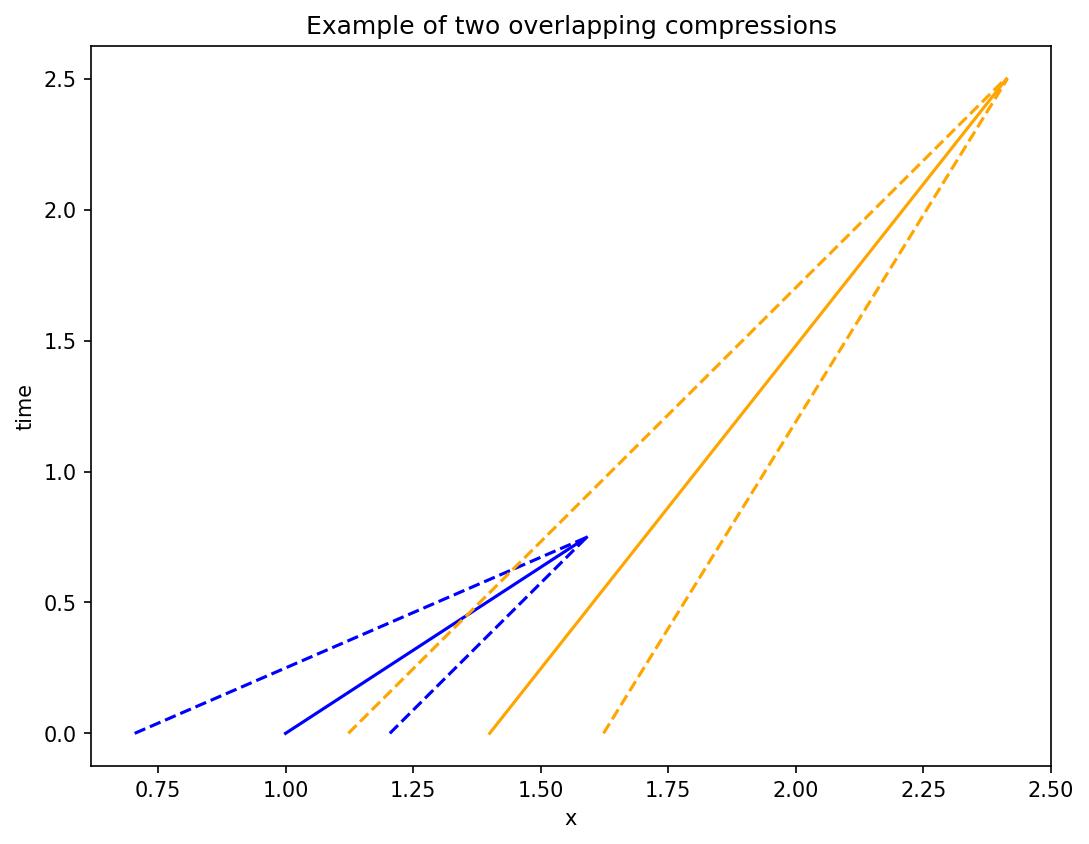
To this end, let’s consider two waves meeting at the origin. Let the leftmost and rightmost states be $U_{l},U_{r}$ respectively, see Figure. Each wave carries two additional pieces of information, the width and a binary value indicating if it’s a shock or a simple wave. Denote these width functions by $w_{l},w_{r}$ and shock indicator functions by $\chi_{l},\chi_{r}$, respectively. The parameters of the $N$ outgoing waves are denoted by $w_{i},\chi_{i}$, $i=1,\ldots,N$. The width of a wave is measured horizontally on the $x-t$ plane, that is, along a constant time. Also, $w_{l/r}\equiv 0$ if $\chi_{l/r}=1$, since a shock has zero width. There could be three cases:
Case 1: If for both waves, width at $t=0$ is zero, then width of all outgoing waves $w_{i}=0$, at the origin, and it is solved as a usual Riemann Problem. The respective values of $\chi_{i}$’s are assigned in accordance with the resolution of the Riemann Problem. An example of this could be a shock-shock, shock-compression, or compression-compression with the width of compression(s) at $t=0$ being zero. The states are resolved as in the beginning of Section 1.2.
Case 2: A more interesting case is (WLOG) $\chi_{l}=1$, $\chi_{r}=0$, with $w_{r}(0)>0$. Also, let’s denote the family of shock (left wave) as $c^{l}$ and the simple wave (right) as $c^{r}$. Then, we set $w_{c_{l}}=0$ imposing that the outgoing wave of the $c^{l}$ family will have zero width. For $i\neq c^{l}$, $\chi_{i}=0$ and $w_{i}(0)=w_{r}(0)$ (zero width for contacts). Therefore, we use compressions instead of shocks for waves of other families. See Figure for a picture of this interaction. This is the resolution of this extended Riemann Problem. Therefore, whether to use simple wave curves or shock wave curves depends on the widths and shock indicator functions.
Case 3: Now suppose $\chi_{l}=0=\chi_{r}$ along with $0<w_{l}(0)<w_{r}(0)$. Then $\chi_{i}=0$ and $w_{i}(0)=w_{r}(0)$ (except contacts which have zero width). Let’s say the states after the interaction are $U^{0},U^{1},\ldots,U^{N}$, where $U^{0}=U_{l},U^{N}=U_{r}$. Then $U^{i}\in\mathcal{W}^{i}(U^{i-1})$ for $i=1,2,\ldots,N$.

Now we fix some notations. Define $\mathcal{Q}^{t}$ to be the complete wave sequence at time $t$ consisting of the sequence $\{\mathcal{Q}^{t}_{j}\}_{j=1}^{J_{t}}$. It is well-known that a key issue in FT algorithms, for larger than $2\times 2$ systems, is to avoid infinitely many waves in finite time. To ensure this, we will make modifications in our scheme later to ensure $\mathcal{Q}^{t}$ is a finite set for each time under some reasonable assumptions. The cardinality ($J_{t}$) depends on time, which is expected since interactions happen as time progresses leading to the increase in the number of waves. Each $\mathcal{Q}^{t}_{j}$ is a set consisting of the following parameters for $j$-th wave (count starts from the left) at time $t$:

$$\mathcal{Q}^{t}_{j}=(c^{j},Z_{j},w_{j},\chi_{j},(x_{j},t_{j}),\sigma_{j},\nu^{j}_{l},\nu^{j}_{r},t^{j}_{s}).$$ (20)

where $c^{j}$ is the family, $Z_{j}$ is the strength, $w_{j}$ is the width (which is a function of time for simple waves and zero for shocks), $\chi_{j}$ is the shock indicator function ($1$ for shock and 00 for simple wave), $(x_{j},t_{j})$ is the point of origin of the wave, $\sigma_{j}$ is the speed, $\nu^{j}_{l},\nu^{j}_{r}$ are the left and right states respectively, and $t^{j}_{s}$ is the self-interaction time. Apart from storing the left, right states associated with the wave, we also denote the complete state sequence by,

$\displaystyle\mathcal{T}^{t}=\{\nu_{j}\}_{j=0}^{J_{t}}.$ (21)

The self-interaction time is only defined for simple waves and may be considered $\infty$ for shocks. We will give more detail about the self interactions later. Some quantities in (20) can be found out in terms of others. For example, from (12),

$\displaystyle\sigma_{j}=\frac{\left(f(\nu_{r}^{j})-f(\nu_{l}^{j})\right)\cdot\left(\nu_{r}^{j}-\nu_{l}^{j}\right)}{\left(\nu_{r}^{j}-\nu_{l}^{j}\right)\cdot\left(\nu_{r}^{j}-\nu_{l}^{j}\right)}.$ (22)

An example of a wave $\mathcal{Q}^{t}_{j}$ is given in Figure. The wave (on the $x-t$ plane) is a line segment,

$\displaystyle x-x_{j}=\sigma_{j}(t-t_{j}),\quad t\in[t_{j},\tau],$ (23)

where $\tau>t_{j}$ is any time before the wave interacts. As mentioned before, if $\chi_{j}=0$, then it has an inherent width that it carries with itself given by $w_{j}$, which changes with time according to (18) and $w_{j}(t_{j})$, which is the width at the point of origin. Note that we will interchangeably use $w_{j}$ as a (width) function of time or to denote the width at a specified time. It will be clear from context as to what is being referred to by $w_{j}$. As for an example, suppose $\mathcal{Q}^{t}_{j}$ is a compression. Its width is then given by,

$$w_{j}=w_{j}(t_{j})+\big{(}\lambda^{c^{j}}(\nu^{j}_{r})-\lambda^{c^{j}}(\nu_{l}^{j})\big{)}\,(t-t_{j}),$$

where the constant $w_{j}(t_{j})$ would be known from the resolution of the interaction when this compression was generated, which was at $(x_{j},t_{j})$.

Again the speed of the jump is taken to be the least square value (12), so is exact for shocks and contacts, and in that case there is zero contribution to the residual, (12).

For a compression, we declare the time at which its width vanishes to be a new interaction time, also to be referred as the self-interaction time $t_{s}^{j}$, namely when the compression collapses and results in a usual Riemann Problem. To this end, we have two types of self-interactions: splitting a rarefaction and collapse of a compression.

We make an important assumption that all the simple waves in our construction are centered. This means that the line of discontinuity as in (23), if extended, passes through the intersection point of the (virtual) left and right edges constituting the width. The width of a simple wave is essentially a virtual blanket around that wave with a virtual left edge and a virtual right edge, see Figure. These virtual edges of the width travel at the respective (left and right of wave) characteristic speeds leading to the total change in width being given by (18). For a simple wave $\mathcal{Q}^{t}_{j}$, suppose $(x_{c},t_{c})$ is the virtual center. Then the virtual left and right edges of the width fall on the lines,

$\displaystyle x-x_{c}=\lambda^{c^{j}}(\nu_{l}^{j})(t-t_{c}),$
$\displaystyle x-x_{c}=\lambda^{c^{j}}(\nu_{r}^{j})(t-t_{c}),$

respectively. It must be that the wave itself must pass through $(x_{c},t_{c})$, that is, this point lies on the line (23). Note that $t_{c}$ need not be in the mentioned interval in (23). Moreover, if the width of the wave is divided into left and right parts, $w_{j}=w_{j}^{L}+w_{j}^{R}$, one on each side of the wave, then it must be that,

$\displaystyle w_{j}^{L}=(\sigma_{j}-\lambda^{c^{j}}(\nu_{l}^{j}))(t-t_{c}),\qquad w_{j}^{R}=(\lambda^{c^{j}}(\nu_{r}^{j})-\sigma_{j})(t-t_{c}).$

This leads to the following important conclusion,

$\displaystyle\frac{w_{j}^{L}}{w_{j}^{R}}=\frac{\sigma_{j}-\lambda^{c^{j}}(\nu_{l}^{j})}{\lambda^{c^{j}}(\nu_{r}^{j})-\sigma_{j}},$ (24)

for all times as long as the existence of this wave.

We ensure that the widths and strengths of simple waves in our scheme is upper bounded by some constant depending on the discretization parameter $\epsilon$. This implies splitting strong rarefactions into weaker ones at the point where they are generated. Note that, at an interaction, since all outgoing jump approximations emanate from a single point of interaction, we cannot split compressions into smaller waves as we do rarefactions. This would be taken care of by adjusting the width of wave. We will see this in detail later.

1.3. Assumptions

We make some global assumptions.

  1. (1)

    The system (1) is physical, that is, there exists a entropy - entropy flux pair with strictly convex entropy.

  2. (2)

    There is a compact invariant region in which the states lie for all time.

  3. (3)

    The Extended Riemann Problem (XRP) is globally uniquely solvable. Global here means the extent to which the system is strictly hyperbolic.

  4. (4)

    The states on the shock curves satisfy the Lax entropy conditions.

  5. (5)

    The initial data $v(x)$ is a compact perturbation of the Riemann Problem, that is, $v=0$ outside a compact set.

In the realm where wave families are either genuinely nonlinear or linearly degenerate, assumption $(3)$ takes the following form: given any $U_{l}$ in the state space, the function

$$G(Z_{1},Z_{2},\ldots,Z_{n};U_{l}):=\mathcal{X}^{N}(Z_{N};\mathcal{X}^{N-1}(Z_{N-1};\ldots Z_{2};\mathcal{X}^{1}(Z_{1};U_{l})\ldots),$$

is one-one and onto the state space, where $\mathcal{X}^{i}(z;u)$ could be any one of the sets $\mathcal{W}^{i}(u)$ or $\left.W^{i}(z;u)\right|_{z>0}\cup\mathcal{S}^{i}(u)$. A more general condition is entailed in…

Remark 1.7.

Some of the assumptions here may be loosened to allow for more systems and initial data. However, our focus is on physical systems wherein these assumptions are mostly known to hold in the respective regime of hyperbolicity.

1.4. Scheme initialization

We will initialize our scheme by solving multiple modified Riemann Problems. A modified Riemann Problem is (1) with,

$\displaystyle u(x,0)=\left\{\begin{array}[]{cl}U_{l},&x<-\alpha,\\ U_{r},&x>\alpha.\end{array}\right.$

Here, $\alpha$ is any nonnegative number and $\alpha=0$ reduces to a Riemann Problem. We join $U_{l}$ to $U_{r}$ by $N$ simple waves only (rarefactions and compressions). Owing to Assumption (3), this can be done uniquely. Note that we use compressions instead of shocks. More specifically, set $U^{0}=U_{l}$ and $U^{N}=U_{r}$ with $U^{i}\in\mathcal{W}^{i}(U^{i-1})$. This resolution is very similar to Case (3) of the XRP in Section 1.2. If $\lambda^{i}(U^{i-1})>\lambda^{i}(U^{i})$, then $U^{i-1}$ to $U^{i}$ is joined by a compression whereas if $\lambda^{i}U^{i-1})\leq\lambda^{i}(U^{i})$, then $U^{i-1}$ to $U^{i}$ is joined by a rarefaction (or contact in case of linearly degenerate field). It remains to assign a location within the interval $(-\alpha,\alpha)$ and width to each wave.

For any left state $U_{l}$, let

$$B_{\bar{\epsilon}}(U_{l})=\left\{u:|Z_{i}|<\bar{\epsilon},\text{for }U_{r}=u,i=1,2,\ldots,N\right\},$$

where $Z_{i}$ denotes the strength of the $i$-th wave, which here is a simple wave.

Denote the width of the simple waves by $w_{i}$ with $\sum_{i=1}^{N}w_{i}(0)=2\alpha$. To initialize our scheme, let’s consider giving equal width to all the $N$ waves that is, $w_{i}(0)=2\alpha/N$. Each wave is placed such that it is centered and all the virtual widths align perfectly with zero overlap at $t=0$, see Figure. The left and right edges of the virtual width travel at the respective (left and right of wave) wavespeeds and therefore, the change in width is given by (18). Since by (12), the wavespeed is a function of adjacent states only, then these two conditions fix the wave location and the profile of the solution. To see this, we perform some calculations to find the location of each wave at $t=0$. Since each wave is given equal width within the interval $[-\alpha,\alpha]$, the virtual width of the $i$-th wave spans the interval,

$$\left(-\alpha+(i-1)\frac{2\alpha}{N},-\alpha+i\frac{2\alpha}{N}\right).$$

Using this and (24), we can find out the size of the left portion of the width for each wave at $t=0$,

$\displaystyle w_{i}^{L}$ $\displaystyle=w_{i}(0)\left(\frac{\sigma_{i}-\lambda^{i}(U^{i-1})}{\lambda^{i}(U^{i})-\lambda^{i}(U^{i-1})}\right)$
$\displaystyle=\frac{2\alpha}{N}\left(\frac{\sigma_{i}-\lambda^{i}(U^{i-1})}{\lambda^{i}(U^{i})-\lambda^{i}(U^{i-1})}\right).$

where $\sigma_{i}$ is the wavespeed as calculated by (12). Adding this to the left edge point of each wave at $t=0$ gives the location of the wave,

$\displaystyle x_{i}=-\alpha+\frac{2\alpha}{N}i-\frac{2\alpha}{N}\left(\frac{\lambda^{i}(U^{i})-\sigma_{i}}{\lambda^{i}(U^{i})-\lambda^{i}(U^{i-1})}\right),\quad(t=0),$ (25)

The waves (or discontinuities) move along the respective lines $x-x_{i}=\sigma_{i}t$ until an interaction takes place. Any compression might collapse to form a shock, which is treted as another interaction. By construction, the left (virtual) edge of the $1$-wave begins at $(-\alpha,0)$, the right (virtual) edge of the $N$-wave begins at $(\alpha,0)$, and all the widths align at $t=0$ with zero overlap, see Figure. In this situation, the first interaction must be a collapse of compression. If there are no compressions, then there are no further interactions and the rarefactions persist for all time.

Using this modified Riemann Problem, we will now initialize the scheme. We will denote the Front Tracking approximate solution by $\widehat{U}^{\epsilon}=\widehat{U}^{\epsilon}(x,t)$ for a discretization parameter $\epsilon>0$. Assumption 1 ensures there is an upper bound on the absolute wave speed for all time, say $\lambda_{max}$. Let $T$ be the time upto which we wish to evolve our scheme. Let $supp(v_{x})\subset(-a,a)$. Take bounded interval $O\subset\mathbb{R}$ with $(-a-\lambda_{max}T,a+\lambda_{max}T)\subset\subset O$. Set boundary data,

$$\left.\widehat{U}\right|_{\partial O}(\cdot,t)=\left\{\lim_{x\to-\infty}v(x),\lim_{x\to\infty}v(x)\right\},\quad t\in[0,T].$$

We will choose $y_{0}<y_{1}<\ldots<y_{\bar{p}}$ which is the partition of $O$ with $y_{0},y_{\bar{p}}$ being the left and right endpoints respectively. The partition must be such that,

  1. (1)

    $y_{p}-y_{p-1}\leq\epsilon^{p_{r}}/2$.

  2. (2)

    All discontinuities in $v$ that generates shocks stronger than $\epsilon^{p_{r}}$ must be in the partition. These are finitely many since the initial data is $BV$. Let $D=\{y_{p_{1}},y_{p_{2}},\ldots y_{p_{k}}\}$ be the set of points of selected discontinuities.

  3. (3)

    For any grid point $y_{p}\notin D$, $v(y_{p})\in B_{\epsilon^{p_{r}}}(v(y_{p-1}^{+}))$ and $v(y_{p+1}^{-})\in B_{\epsilon^{p_{r}}}(v(y_{p}))$. This is possible owing to continuity of initial data in those intervals.

At the points in $D$, we solve a usual Riemann Problem to generate waves, which are either shocks or rarefactions (centered with zero starting width). Any rarefactions stronger than $\epsilon^{p_{r}}$ are split as discussed in Section 1.1, such that the strength of each is less than $\epsilon^{p_{r}}$.

For other points in the partition, we solve a modified Riemann Problem on each interval $[y_{p-1},y_{p}]$, with left and right states $v(y_{p-1}),v(y_{p})$ (or the respective limits in case one or more of the points is in $D$) respectively, as discussed in the beginning of this section, with $\alpha=(y_{p}-y_{p-1})/2$ and origin being $(y_{p}+y_{p-1})/2$. We then have the location of each wave in the interval $(y_{p-1},y_{p})$ through (25). In this way, we have shocks, rarefactions and compressions at $t=0^{+}$, with all the simple waves having strength less than $\epsilon^{p_{r}}$. Using the notation in (20), (21), the discrete wave sequence can now be written as,

$$\widehat{U}^{\epsilon}(x,t):=\nu_{0}+\sum_{j}(\nu_{j}-\nu_{j-1})H(x-x_{j}-\sigma_{j}t),$$

until the first time of interaction. The discrete solution evolves and an XRP is solved whenever two waves meet. The times upto which the scheme is well-defined, all the interaction times can be calculated exactly. Subsequently, the interactions happen in the correct order and the interaction time list is updated after each interaction.

Remark 1.8.

Owing to (12), we are treating shocks exactly and have (small) error in the simple waves. This can be seen as an error adjustment for the consideration of strong waves, namely, where the approximate solution is bad (which is at shocks), we treat it exactly, and where it is good ($C^{2}$ at simple waves), we make small errors.

Now, we move on to describing some special interactions/features exclusive to our scheme that are needed especially for consistency involving large amplitude waves.

1.4.1. Avoiding adjacent simple waves width overlap

This section also makes sure that compressions of same family do not collide without one of them collapsing first.

When any simple wave originates (with nonzero width) right after an interaction, we check two conditions,

  1. (1)

    If there is another simple wave of the same family right adjacent to it.

  2. (2)

    If the virtual widths of the two waves overlap.

If both the conditions hold then we make some changes. If any one of them fails, things stay as it is. We perform the procedure described in this section right after an interaction, when a simple wave of nonzero width is produced. Of all the adjustments entailed in further sections, that are performed immediately after an interaction, this is given the highest precedence. Also, almost always, condition (1) would be satisfied at most on one side of the newly generated wave, since a generic interaction would produce $N$ waves of $N$ different families. However, this procedure works otherwise too. Only that we would follow the algorithm twice.

Suppose a newly generated simple wave (of nonzero width) at an interaction at $t=t_{j}$,

$$(c^{j},Z_{j},w_{j},0,(x_{j},t_{j}),\sigma_{j},\nu_{l},\nu_{m},t^{j}_{s}),$$

and suppose there is another simple of the same family to the right,

$$(c^{j},Z_{j+1},w_{j+1},0,(x_{j+1},t_{j+1}),\sigma_{j+1},\nu_{m},\nu_{r},t^{j+1}_{s}),$$

with $t_{j+1}<t_{j}$. By assumption, both waves are centered. In case of compression(s), the center(s) are the respective point(s) of collapse. Let

$$w_{j}(t_{j})=w_{j}^{R}+w_{j}^{L},\qquad w_{j+1}(t_{j})=w_{j+1}^{R}+w_{j+1}^{L},$$

the respective left and right portions of the total width of each wave at $t=t_{j}$. From this point onwards, until the end of Section 1.4.1, we omit the dependence of width functions on time and all $w$’s with various super/subscripts denote widths at $t=t_{j}$. So, we will denote $w_{j}(t_{j}),w_{j+1}(t_{j})$ as $w_{j},w_{j+1}$.

Suppose the $(j+1)$-th wave passes through $(\bar{x}_{j+1},t_{j})$, that is, the location of the wave at the time when the $j$-th wave is generated. If the following holds,

$$\bar{x}_{j+1}-x_{j}<w_{j}^{R}+w_{j+1}^{L},$$

then there is an overlap of widths. From (24), this condition is equivalent to,

$\displaystyle\bar{x}_{j+1}-x_{j}<\left(\frac{\sigma_{j}-\lambda(\nu_{m})}{\lambda(\nu_{l})-\lambda(\nu_{m})}\right)w_{j}+\left(\frac{\lambda(\nu_{m})-\sigma_{j+1}}{\lambda(\nu_{m})-\lambda(\nu_{r})}\right)w_{j+1}.$ (26)

We drop the notation signifying the dependence of the eigenvalue on the family since in this section, we need to only consider single wave family at a time.

Refer to caption
Figure 1. Two compressions with overlapping widths.

Set the overlap as,

$$E=w_{j}^{R}+w_{j+1}^{L}-(\bar{x}_{j+1}-x_{j}),$$

We will modify the width of the two waves so as to remove the overlap. While doing this, we should note what would have had happened physically. The overlap that occurs is like an error that should not have occured in the actual solution. Also, an overlap in two compressions signifies that shocks may have been present somewhere. Keeping this in mind, we reduce the width of the two simple waves in the following manner: the right width of left wave and the left width of right wave are changed so that they align; these new widths are distributed to each in proportion of their respective original widths. So,

$$w_{j}^{R,New}+w_{j+1}^{L,New}=\bar{x}_{j+1}-x_{j},\qquad\text{and,}\qquad\frac{w_{j}^{New}}{w_{j+1}^{New}}=\frac{w_{j}}{w_{j+1}}.$$

Here, the superscript $New$ denotes the new widths at $t=t_{j}$ and $L,R$ the left and right widths respectively. Consequently, using (24),

$$\left(\frac{\sigma_{j}-\lambda(\nu_{m})}{\lambda(\nu_{l})-\lambda(\nu_{m})}\right)w_{j}^{New}+\left(\frac{\lambda(\nu_{m})-\sigma_{j+1}}{\lambda(\nu_{m})-\lambda(\nu_{r})}\right)w_{j+1}^{New}=\bar{x}_{j+1}-x_{j},$$

and using this in the preceding equation,

$$w_{j}^{New}=\left[\left(\frac{\sigma_{j}-\lambda(\nu_{m})}{\lambda(\nu_{l})-\lambda(\nu_{m})}\right)+\left(\frac{\lambda(\nu_{m})-\sigma_{j+1}}{\lambda(\nu_{m})-\lambda(\nu_{r})}\right)\frac{w_{j+1}}{w_{j}}\right]^{-1}(\bar{x}_{j+1}-x_{j}).$$
$$w_{j+1}^{New}=\left[\left(\frac{\sigma_{j}-\lambda(\nu_{m})}{\lambda(\nu_{l})-\lambda(\nu_{m})}\right)\frac{w_{j}}{w_{j+1}}+\left(\frac{\lambda(\nu_{m})-\sigma_{j+1}}{\lambda(\lambda_{m})-\lambda(\nu_{r})}\right)\right]^{-1}(\bar{x}_{j+1}-x_{j}).$$

The expression in the inverse is always positive no matter the wave is compressive or rarefactive.

[Uncaptioned image]

Consequently, the waves align exactly and the common virtual edge travels with speed, $\lambda(\nu_{m})$. This process can be carried out for any two adjacent simple waves in case of overlap. By induction, we have the following Lemma.

Lemma 1.9.

For any sufficiently small discretization parameter and as long as the scheme construction is well-defined, there are no overlapping adjacent simple waves of same family in the scheme.

1.4.2. Rarefaction splitting to limit width or strength

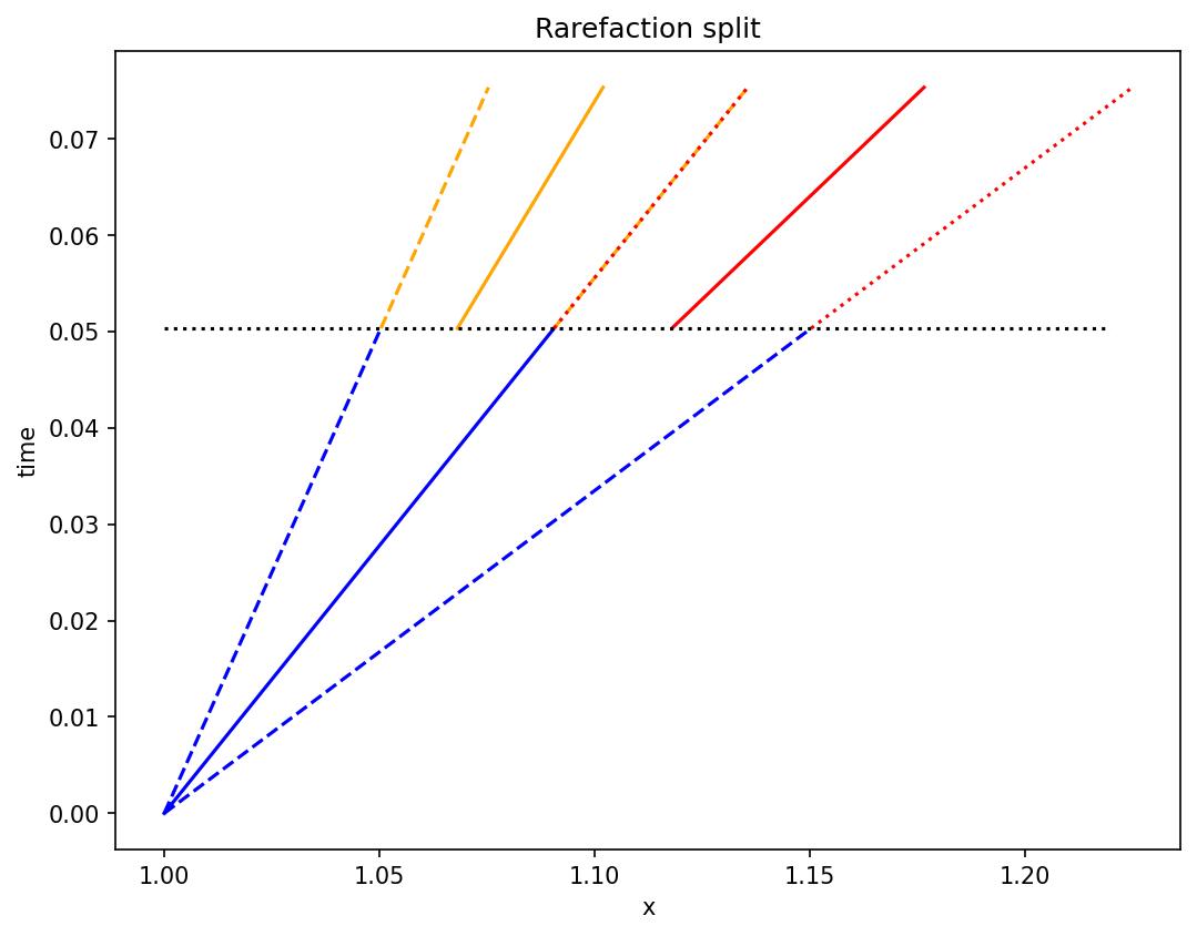
We would be requiring to split rarefactions in two cases: when it is too wide or when its strength increases by a large factor after an interaction. The basic idea remains the same for both situations. In case the rarefaction achieves a threshold width, we split it into two. However, in case of splitting to limit strength, we will need a mechanism to split it into multiple pieces, as it is not known a priori how much the strength would increase by, after an interaction. So, we will describe a general split of a rarefaction wave into $m$ smaller splits. To this end, suppose a rarefaction wave of family $c$ and with eigenvalue $\lambda$ as,

$$(c,Z,w,0,(x_{j},t_{j}),\sigma,\nu_{l},\nu_{r},t^{j}_{s}),$$

with width,

$$w=w_{int}+(\lambda(\nu_{r})-\lambda(\nu_{l}))(t-t_{0}),$$

where $t_{0}$ is the time of split. Hence, $w_{int}$ is the width at the time of split. Suppose the wave passes through $(x_{0},t_{0})$. Using (24), let

$\displaystyle x_{0}^{L}:=x_{0}-\left(\frac{\sigma-\lambda(\nu_{l})}{\lambda(\nu_{r})-\lambda(\nu_{l})}\right)w_{int},$
$\displaystyle x_{0}^{R}:=x_{0}+\left(\frac{\lambda(\nu_{r})-\sigma}{\lambda(\nu_{r})-\lambda(\nu_{l})}\right)w_{int},$

be the (virtual) left and right edges of the width at $t=t_{0}$. See Figure for reference.

Next, we choose $m-1$ states, $\nu_{1},\nu_{2},\ldots,\nu_{m-1}$, on the wave curve such that,

$$\lambda(\nu_{l})=:\lambda(\nu_{0})<\lambda(\nu_{1})<\ldots<\lambda(\nu_{m-1})<\lambda(\nu_{m}):=\lambda(\nu_{r}).$$

At this point, we do not assume any other condition in choosing the states, which leaves us with a lot of freedom to choose from. However, more conditions will be levied on the choice of states depending on whether we are splitting to reduce width or strength. As of now, we describe the general part of the procedure, that would be followed for both situations.

We define a new temporary wave called a multi-rarefaction. It is temporary in the sense that it only has a short time of existence. When the split starts at $t=t_{0}$, the rarefaction wave will temporarily convert into multi-rarefaction. This wave will have two parts: a propagating background, which is not a part of the actual FT approximate solution, and the actual propagating discontinuities. The temporary multi-rarefaction ends when these two parts coincide. First, we describe the propagating background.

This part is composed of what the splitted rarefaction would be in case infinite speed of propagation was allowed. It is composed of $m$ waves in between the states $\nu_{k}$’s. The wavespeed of the wave in between states $\nu_{k-1},\nu_{k}$ is given by (12), call the wavespeeds, $\sigma_{k}$, $k=1,\ldots,m$. As a result, a single rarefaction is divided into $m$ waves, however, the position of the waves is to be found. The position is obtained by imposing that the wave before split and the splitted parts are all centered with the same center, see Figure. The virtual center of the rarefaction can be found out as the intersection of the lines, $x-x_{0}^{L}=\lambda(\nu_{l})(t-t_{0})$ and $x-x_{0}^{R}=\lambda(\nu_{r})(t-t_{0})$, which turns out to be,

$\displaystyle(x_{c},t_{c}):=\left(\frac{\lambda(\nu_{r})x_{0}^{L}-\lambda(\nu_{l})x_{0}^{R}}{\lambda(\nu_{r})-\lambda(\nu_{l})},t_{0}-\frac{x_{0}^{R}-x_{0}^{L}}{\lambda(\nu_{r})-\lambda(\nu_{l})}\right).$

Hence, each split (wave) in the propagating background falls on the line $x-x_{c}=\sigma_{k}(t-t_{c})$ for $t>t_{0}$. Therefore, each wave emanates from the point,

$\displaystyle(x_{0}^{k},t_{0}):=\left(\frac{x_{0}^{R}(\sigma_{k}-\lambda(\nu_{l}))+x_{0}^{L}(\lambda(\nu_{r})-\sigma_{k})}{\lambda(\nu_{r})-\lambda(\nu_{l})}\right).$

By construction, $x_{0}^{L}<x_{0}^{1}<\ldots<x_{0}^{m}<x_{0}^{R}$. Our construction also ensures just the right amount of widths without overlap, so that all the splitted components along with their virtual widths align perfectly. To see this, let’s suppose the width given to each wave at $t=t_{0}$ is,

$$w_{k}=w_{k}^{L}+w_{k}^{R},$$

with $w_{k}^{L},w_{k}^{R}$ being the left and right parts respectively of the total width of the $k$-th split. Firstly, we impose that,

$\displaystyle w_{1}^{L}$ $\displaystyle=x_{0}^{1}-x_{0}^{L}$
$\displaystyle=\left(\frac{x_{0}^{R}-x_{0}^{L}}{\lambda(\nu_{r})-\lambda(\nu_{l})}\right)(\sigma_{1}-\lambda(\nu_{l})).$

Owing to (24), we can obtain $w_{1}^{R}$ from $w_{1}^{L}$ as,

$\displaystyle w_{1}^{R}$ $\displaystyle=\left(\frac{\lambda(\nu_{1})-\sigma_{1}}{\sigma_{1}-\lambda(\nu_{l})}\right)w_{1}^{L}$
$\displaystyle=\left(\frac{x_{0}^{R}-x_{0}^{L}}{\lambda(\nu_{r})-\lambda(\nu_{l})}\right)(\lambda(\nu_{1})-\sigma_{1}).$

Note that,

$$x_{0}^{k}-x_{0}^{k-1}=\left(\frac{x_{0}^{R}-x_{0}^{L}}{\lambda(\nu_{r})-\lambda(\nu_{l})}\right)(\sigma_{k}-\sigma_{k-1}).$$

To ensure that the splitted rarefactions exactly align, we impose,

$$w_{2}^{L}=x_{0}^{2}-x_{0}^{1}-w_{1}^{R}.$$

Through (24) once again, we can obtain $w_{2}^{R}$. In fact, continuing in this way, we can inductively show,

$\displaystyle w_{k}^{L}=\left(\frac{x_{0}^{R}-x_{0}^{L}}{\lambda(\nu_{r})-\lambda(\nu_{l})}\right)(\sigma_{k}-\lambda(\nu_{k-1})).$

Indeed, using (24),

$$w_{k}^{R}=\left(\frac{x_{0}^{R}-x_{0}^{L}}{\lambda(\nu_{r})-\lambda(\nu_{l})}\right)(\lambda(\nu_{k})-\sigma_{k}).$$

Consequently,

$\displaystyle w_{k+1}^{L}$ $\displaystyle=x_{0}^{k+1}-x_{0}^{k}-w_{k}^{R}$
$\displaystyle=\left(\frac{x_{0}^{R}-x_{0}^{L}}{\lambda(\nu_{r})-\lambda(\nu_{l})}\right)(\sigma_{k+1}-\lambda(\nu_{k})).$

Also, the total width at $t=t_{0}$ is,

$\displaystyle w_{k}=w_{k}^{L}+w_{k}^{R}=\left(\frac{\lambda(\nu_{k})-\lambda(\nu_{k-1})}{\lambda(\nu_{r})-\lambda(\nu_{l})}\right)w_{int}.$ (27)

Note that by construction, all the widths are positive and therefore, well-defined. Moreover, through $w_{m}^{L}$ as calculated above, we can use (24) again to get,

$\displaystyle w_{m}^{R}$ $\displaystyle=\left(\frac{\lambda(\nu_{r})-\sigma_{m}}{\sigma_{m}-\lambda(\nu_{m-1})}\right)w_{m}^{L}$
$\displaystyle=\left(\frac{x_{0}^{R}-x_{0}^{L}}{\lambda(\nu_{r})-\lambda(\nu_{l})}\right)(\lambda(\nu_{r})-\sigma_{m})$
$\displaystyle=x_{0}^{R}-x_{0}^{m}.$

Therefore, the sum of all the widths at $t_{0}$ is the original width (before split) and the individual widths align exactly. Since the virtual edges move with characterstic speeds, all the calculated widths have zero overlap for $t>t_{0}$.

This propagating background part of the multi-rarefaction wave is now augmented with the actual propagating discontinuities. In this part, for $t>t_{0}$, there are $m$ discontinuities emanating from $(x_{0},t_{0})$. These discontinuities, which are the actual splits, map one to one to the wave splits in the background as discussed above. Fix some positive $\theta<1$. The wavespeeds of the splits are,

$\displaystyle\mu_{k}:=\left\{\begin{array}[]{lr}\sigma_{k}-|\lambda(\nu_{k})-\lambda(\nu_{k-1})|^{\theta},&\text{if }\sigma_{k}<\sigma,\\ \sigma_{k}+|\lambda(\nu_{k})-\lambda(\nu_{k-1})|^{\theta}&\text{if }\sigma_{k}>\sigma,\\ \sigma&\text{if }\sigma_{k}=\sigma,\end{array}\right.$ (31)

for $k=1,\ldots,m$. Owing to the way $\mu_{k}$’s are defined, there exists some finite time when the $k$-th wave of the background propagation part meets the $k$-th wave of the actual propagating discontinuities. The importance of the extra terms in the first two branches is to make this happen quicker, in particular, smaller the discretization parameter $\epsilon$, faster the background part meets the actual propagating discontinuities. We can calculate the time as follows,

$\displaystyle\bar{t}_{k}$ $\displaystyle:=t_{0}+\left|\frac{x_{k}^{0}-x_{0}}{\sigma_{k}-\mu_{k}}\right|$
$\displaystyle=t_{0}+\left|\frac{\frac{x_{0}^{R}(\sigma_{k}-\lambda(\nu_{l}))+x_{0}^{L}(\lambda(\nu_{r})-\sigma_{k})}{\lambda(\nu_{r})-\lambda(\nu_{l})}-x_{0}}{\sigma_{k}-\mu_{k}}\right|$
$\displaystyle=t_{0}+\left|\frac{\sigma_{k}(x_{0}^{R}-x_{0}^{L})-\lambda(\nu_{l})(x_{0}^{R}-x_{0})-\lambda(\nu_{r})(x_{0}-x_{0}^{L})}{(\lambda(\nu_{r})-\lambda(\nu_{l}))(\sigma_{k}-\mu_{k})}\right|$
$\displaystyle=t_{0}+w_{int}\left|\frac{\sigma_{k}(\lambda(\nu_{r})-\lambda(\nu_{l}))-\lambda(\nu_{l})(\lambda(\nu_{r})-\sigma)-\lambda(\nu_{r})(\sigma-\lambda(\nu_{l}))}{(\lambda(\nu_{r})-\lambda(\nu_{l}))^{2}(\sigma_{k}-\mu_{k})}\right|$
$\displaystyle=t_{0}+\frac{w_{int}}{|\sigma_{k}-\mu_{k}|}\frac{|\sigma_{k}-\sigma|}{(\lambda(\nu_{r})-\lambda(\nu_{l}))}.$ (32)

Note that the actual propagating discontinuities have wavespeeds within the wavespeed bounds of that family upto $O(\epsilon^{p_{r}\theta})$. In particular, if this split happens right after an interaction, then owing to hyperbolicity, there are no spurious interactions with the waves of any other family generated at the interaction.

Now we state as to when the temporary multi-rarefaction ends to give $m$ separate rarefaction waves. Suppose that there are no other waves that interact with the first and the last ($m$-th) wave of the actual propagating discontinuities, until time $t_{\#}:=\max_{k}\{\bar{t}_{k}\}$. Then, as and when each wave is incident on the corresponding background wave, its wavespeed ($\mu_{k}$) is tweaked to $\sigma_{k}$. So, for $t\geq\bar{t}_{k}$, the $k$-th wave in the propagating background and the actual propagating discontinuities part coincide. In this way, at $t=t_{\#}$, both the parts of the multi-rarefaction coincide completely. From $t>t_{\#}$, the wave is no more a multi-rarefaction but $m$ separate waves, each with its own parameters as in (20). The waves travel thus and interact through our set rules.

However, it could be that there is another wave coming in that interacts with the first or the last ($m$-th) wave of the actual propagating discontinuities, before $t_{\#}$, say at $t=t_{\ast}>t_{0}$. Call this interaction the outer interaction. In this case, we instantly tweak the wavespeeds of all constituent waves from $\mu_{k}$ to $\sigma_{k}$ and perform some manipulations to the widths of each of those at $t_{\ast}^{-}$, that is, right before the interaction. The location of the waves at $t_{\ast}$ is,

$$x_{\ast}^{k}:=x_{0}+\mu_{k}(t_{\ast}-t_{0}),\qquad k=1,2,\ldots,m.$$

Also, the outer interaction either happens at $x_{\ast}^{1}$ or $x_{\ast}^{m}$. Without loss of generality, let’s say it happens at $x^{m}_{\ast}$. Hence, the actual propagating discontinuities after $t_{\ast}$ would be,

$$x-x^{k}_{\ast}=\sigma_{k}(t-t_{\ast}),\qquad k=1,2,\ldots,m-1,$$

and the $m$-th wave interacts to generate new waves according to the corresponding extended Riemann Problem. The only thing that remains is to assign widths to each of those $m$ waves at $t_{\ast}^{-}$. Firstly, note that until this time, the background propagating discontinuities has width spanning $[x_{\ast}^{L},x_{\ast}^{R}]$ where,

$\displaystyle x_{\ast}^{L}=x_{c}+\lambda(\nu_{l})(t_{\ast}-t_{c}),\qquad x_{\ast}^{R}=x_{c}+\lambda(\nu_{r})(t_{\ast}-t_{c}).$

We assign widths, $w_{\ast}^{k}=w_{\ast}^{k,L}+w_{\ast}^{k,R}$, at $t_{\ast}$ according to the following optimization problem,

$\displaystyle\begin{aligned} &\min x_{\ast}^{R}-x_{\ast}^{L}-\sum_{k=1}^{m}w_{\ast}^{k},\\ &w_{\ast}^{k}>0,\quad k=1,2,\ldots,m,\\ &w_{\ast}^{1,L}\leq x_{\ast}^{1}-x_{\ast}^{L},\\ &\left(\frac{\lambda(\nu_{k})-\sigma_{k}}{\sigma_{k}-\lambda(\nu_{k-1})}\right)w_{\ast}^{k,L}+w_{\ast}^{k+1,L}\leq x_{\ast}^{k+1}-x_{\ast}^{k},\ k=1,2,\ldots m-1\\ &\left(\frac{\lambda(\nu_{r})-\sigma_{m}}{\sigma_{m}-\lambda(\nu_{m-1})}\right)w_{m}^{L}\leq x_{\ast}^{R}-x_{\ast}^{m},\end{aligned}$ (33)

where the first term in the third constraint inequality is in fact $w_{\ast}^{k,R}$, in terms of $w_{\ast}^{k,L}$, using (24). Similarly, in the last constraint, the expression on the left is $w_{\ast}^{m,R}$.

Remark 1.10.

The optimization problem (33) is a very precise way of choosing the widths so as to minimize the error due to widths. However, we could just choose any widths $w_{\ast}^{k}>0$ satisfying the given constraints (that is guaranteed to exist). This would not make much of a difference since correction due to widths is higher order, and would go to zero as $\epsilon$ goes to zero.

Once these widths are assigned, the $k$-th wave (except $k=m$) have rate of change of widths as,

$$\lambda(\nu_{k})-\lambda(\nu_{k-1}).$$

Since there is no overlap at $t=t_{\ast}$ owing to our constraints, there is no overlap between these waves for later times. The $m$-th and the other incoming wave constitute the outer interaction and are resolved to generate new waves.

This is our mechanism to split a rarefaction into multiple smaller ones. Now we apply our mechanism to limit the width and strength.

  • Width: We set a rule that we must split a rarefaction into two rarefactions anywhere in between width range $3\epsilon^{p_{r}}/4$ to $\epsilon^{p_{r}}$. Allowing this range enables us to choose a time away from any other adjacent approaching wave as much as possible. For convenience, the middle state $\nu_{m}$ is chosen to be such that it satisfies the equation $\lambda(\nu_{m})=\sigma$, the wavespeed of the rarefaction before the split. Following notation from previous discussion, let $t_{0}$ be the time of the split. Firstly, note that from (32),

    $\displaystyle\bar{t}_{k}-t_{0}$ $\displaystyle=\frac{w_{int}}{|\sigma_{k}-\mu_{k}|}\frac{|\sigma_{k}-\sigma|}{(\lambda(\nu_{r})-\lambda(\nu_{l}))}$
    $\displaystyle\leq\frac{w_{int}}{|\sigma_{k}-\mu_{k}|}$
    $\displaystyle\lesssim O(\epsilon^{(1-\theta)p_{r}}).$ (34)

    The second inequality is true since $\sigma,\sigma_{k}$’s lie within $(\lambda(\nu_{l}),\lambda(\nu_{r}))$. In the last inequality, we used the definition of $\mu_{k}$’s, and the choice of $\nu_{m}$ ensures each splitted component has strength in the order of $\epsilon^{p_{r}}$, along with the fact that all the splitted components have strengths bounded by $\epsilon^{p_{r}}$, which is true since the original rarefaction strength is bounded by the same.

    Moreover, by choosing the middle state as above, we have from (27) that the respective left and right widths of the splits in the background propagation part at $t=t_{0}$ are,

    $$w_{1}=w_{int}\left(\frac{\sigma-\lambda(\nu_{l})}{\lambda(\nu_{r})-\lambda(\nu_{l})}\right),\qquad w_{2}=w_{int}\left(\frac{\lambda(\nu_{r})-\sigma}{\lambda(\nu_{r})-\lambda(\nu_{l})}\right).$$

    Also, $\sigma$ is the wavespeed of the original rarefaction (before split) obtained through (12), which matches on shocks. Moreover, for weak waves, it is well-known (see [Lax57]), that speeds are the average of the left and right characteristic speeds upto second order in strength, and the simple wave curve and shock curves differ at third order. Consequently,

    $$w_{1}=\frac{w_{int}}{2}+O(\epsilon^{2p_{r}}),\qquad w_{2}=\frac{w_{int}}{2}+O(\epsilon^{2p_{r}}),$$

    which in turn implies $w_{k}\leq\epsilon^{p_{r}}/2+O(\epsilon^{2p_{r}})$. Therefore, the times, $t_{s}^{1},t_{s}^{2}$, at which the splitted components again reach splittable widths ($3\epsilon^{p_{r}}/4$) is,

    $\displaystyle t_{s}^{1}-t_{0}$ $\displaystyle\approx\frac{\frac{3\epsilon^{p_{r}}}{4}-\frac{\epsilon^{p_{r}}}{2}+O(\epsilon^{2p_{r}})}{\sigma-\lambda(\nu_{l})}$
    $\displaystyle=\frac{\frac{\epsilon^{p_{r}}}{4}+O(\epsilon^{2p_{r}})}{O(\epsilon^{p_{r}})}$
    $\displaystyle=O(1).$ (35)

    Compare this to (34), we conclude that a multirarefaction must either become 2 separate component rarefactions by reaching time $\max\{\bar{t}_{1},\bar{t}_{2}\}$ or interact with another wave, before any of the two components reach splittable widths again.

  • Strength: This split happens right after an interaction, and only for the generated rarefaction(s) whose strengths increase to more than $\epsilon^{p_{r}}$. Here, there could be multiple splits for each rarefaction to ensure that the strength of each component split is less than $\epsilon^{p_{r}}$. For convenience and consistency, we choose middle states in a way that strengths of the splitted components are close. This avoids unnecessary splits. In particular, we could choose the states that result in equal strength of all the splits. The calculations here are similar as in the splitting to limit width situation. Here, the time of interaction is equal to the time of split $t_{0}$. In particular, the split happens at $t_{0}^{+}$, which is immediately after the interaction. Note once again from (32) that,

    $\displaystyle\bar{t}_{k}-t_{0}$ $\displaystyle=\frac{w_{int}}{|\sigma_{k}-\mu_{k}|}\frac{|\sigma_{k}-\sigma|}{(\lambda(\nu_{r})-\lambda(\nu_{l}))}$
    $\displaystyle\lesssim O(\epsilon^{(1-\theta)p_{r}}).$

    Therefore, multirarefaction terminates and generates individual rarefaction splits faster as $\epsilon$ goes to zero.

Refer to caption
Figure 2. Rarefaction split into two. Solid lines are the actual jump discontinuity (wave) in the scheme. Dotted lines represent the virtual width. In this example, $t_{\ast}=0.05$.

We now give a condition for the eventual decrease in residual in a rarefaction split.

Lemma 1.11.

Suppose the function $\phi(\cancel{z},\bcancel{z})$ as defined in (36) below is such that $\partial_{\cancel{z}}\partial_{\bcancel{z}}\phi(\cancel{z},\bcancel{z})<0$. Then the residual (12) decreases from the starting of the split and at the termination of the multirarefaction.

Lemma 1.11 is a very general condition for the residual decrease and may not be readily checkable. However, building on this result, we will give a clean and easily checkable condition for residual decrease for the p-system, in Section 2.1.

We will show the calculations for split into two. More splits result in even further decrease in the residual. Let’s do some preliminary calculations. We will carry over the notations from our discussion above. The dependence on the wave index and family is omitted as it is not needed. Also, $[\cdot]_{rl}$ represents jump in the quantity across the original rarefaction which has $\nu_{r},\nu_{l}$ as the right and left states respectively. Similarly, we use $[\cdot]_{ml},[\cdot]_{rm}$. Using (12), the residual for a single rarefaction (before split) is,

$\displaystyle|R|_{bef}$ $\displaystyle=\left|[f]_{rl}-\frac{[\nu]_{rl}[\nu]_{rl}^{T}[f]_{rl}}{[u]_{rl}^{T}[u]_{rl}}\right|$
$\displaystyle=\left|\left(I-\frac{[u]_{rl}[u]_{rl}^{T}}{[u]_{rl}^{T}[u]_{rl}}\right)[f]_{rl}\right|$
$\displaystyle=:\left|(I-P_{rl})[f]_{rl}\right|,$

where $P_{rl}=\frac{[u]_{rl}[u]_{rl}^{T}}{[u]_{rl}^{T}[u]_{rl}}$ is a projection matrix. So, we have,

$\displaystyle|R_{bef}|$ $\displaystyle=\sqrt{[f]_{rl}^{T}(I-P_{rl})[f]_{rl}}$
$\displaystyle=\sqrt{[f]_{rl}^{T}[f]_{rl}-\frac{\left([f]_{rl}^{T}[\nu]_{rl}\right)^{2}}{[\nu]_{rl}^{T}[\nu]_{rl}}}$

Since the states are on a simple wave curve, through (4), we have the following,

$$[\nu]_{rl}=\int_{z_{l}}^{z_{r}}r(u(z))\,dz,$$

and

$\displaystyle[f]_{rl}$ $\displaystyle=\int_{z_{l}}^{z_{r}}Df(u(z))\,\frac{du}{dz}\,dz$
$\displaystyle=\int_{z_{l}}^{z_{r}}\lambda(u(z))\,r(u(z))\,dz,$

with $u(z_{l})=\nu_{l},u(z_{r})=\nu_{r}$. Plugging these into the expression for residual above, we obtain,

$\displaystyle|R_{bef}|$ $\displaystyle=\sqrt{\left|\int_{z_{l}}^{z_{r}}\!\!\!\!\!\lambda(u(z))\,r(u(z))\,dz\right|^{2}-\frac{\left(\int\limits_{(z_{l},z_{r})^{2}}\lambda(u(\cancel{z}))\,r^{T}(u(\cancel{z}))\,r(u(\bcancel{z}))d(\cancel{z},\bcancel{z})\right)^{2}}{\left|\int_{z_{l}}^{z_{r}}r(u(z))\,dz\right|^{2}}}$
$\displaystyle=:\phi(z_{l},z_{r}).$ (36)

We can perform similar calculations on each splitted component to obtain the following,

$\displaystyle\Delta R$ $\displaystyle=R_{aft}-R_{bef}$
$\displaystyle=\phi(z_{l},z_{m})+\phi(z_{m},z_{r})-\phi(z_{l},z_{r}),$

with $u(z_{m})=\nu_{m}$, which is the middle state after the split. Also, genuine nonlinearity assumption gives $z_{l}<z_{m}<z_{r}$. We used the group property, (6), of the simple wave curve.
Proof of Lemma. From expression of $\Delta R$ above, and using that $\phi(z_{m},z_{m})=0$, we have

$\displaystyle\Delta R$ $\displaystyle=\phi(z_{l},z_{m})+\phi(z_{m},z_{r})-\phi(z_{l},z_{r})-\phi(z_{m},z_{m})$
$\displaystyle=\int_{z_{l}}^{z_{m}}\int_{z_{m}}^{z_{r}}\partial_{\bcancel{z}}\partial_{\cancel{z}}\phi(\cancel{z},\bcancel{z})\,d\bcancel{z}d\cancel{z}.$

Hence, the result. ∎

1.4.3. Collapse of a compression

This interaction occurs when a simple wave of compressive type (width decreasing with time) attains zero width. This could happen in two situations.

  1. (1)

    The compression naturally attains zero width.

  2. (2)

    There is an interaction between a simple wave and another wave whose resolution would have generated one or more compressions with strength greater than $\epsilon^{p_{c}}$. In such a situation, this concerned interaction is resolved after assigning $w=0$ for the outgoing wave of that family. For systems with ‘well-behaved’ wave/shock curves, this implies imposing the generated wave of that family must be a shock.

Let’s consider the first situation. The resolution of this collapse is in fact the resolution of a simple Riemann Problem. As a result, only shocks, and/or contacts, and/or centered rarefactions are generated. Hence, all rarefactions that are generated have zero width at the time of the self-interaction.

Assume a simple wave of compression type,

$$(c,Z,w,0,(x_{j},t_{j}),\sigma,\nu_{l},\nu_{r},t_{\ast}),$$

with $w=w_{int}+[\lambda^{c}](t-t_{j})$, $w_{int}<\epsilon^{p_{r}}/2$ and for $t_{j}\leq t<t_{\ast}$. The bound on $w_{int}$ can be obtained by an induction on the simple waves, since the way we initialized ensured the bound. Note that $t_{\ast}$ is the self-interaction time and $\dot{w}=\left[\lambda^{c}\right]<0$, $\left[\lambda^{c}\right]:=\lambda(\nu_{r})-\lambda(\nu_{l})$. Also, $w_{int}$ is the width at $t=t_{j}$, the time when the compression is generated in the scheme. Since $t_{\ast}$ is the time of self-interaction, or collapse in this case, it can be explicitly computed,

$$t_{\ast}=t_{j}-\frac{w_{int}}{\left[\lambda^{c}\right]}.$$

The corresponding $x$ coordinate is,

$\displaystyle x_{\ast}$ $\displaystyle=x_{j}+\sigma_{j}(t_{\ast}-t_{j})$
$\displaystyle=x_{j}-\sigma_{j}\frac{w_{int}}{\left[\lambda^{c}\right]}.$

Here, we are assuming (WLOG) that the compression does not interact with any other wave until $t_{\ast}$. After the interaction, there are at least $N$ waves generated of $N$ distinct families (generically). Rarefactions stronger than $\epsilon^{p_{r}}$ are split immediately as discussed in Section 1.1. As for an example here, if all the generated rarefactions are weaker than $\epsilon^{p_{r}}$, we then denote $N$ waves generated as follows,

$\displaystyle(1,Z_{j_{1}},0,\chi_{j_{1}},(x_{\ast},t_{\ast}),\sigma_{j_{1}},\nu_{l},\nu_{1},t_{s}^{1}),$
$\displaystyle(2,Z_{j_{1}+1},0,\chi_{j_{1}+1},(x_{\ast},t_{\ast}),\sigma_{j_{1}+1},\nu_{1},\nu_{2},t_{s}^{2}),$
$\displaystyle\vdots$
$\displaystyle(N,Z_{j_{1}+N-1},0,\chi_{j_{1}+N-1},(x_{\ast},t_{\ast}),\sigma_{j_{1}+N-1},\nu_{N-1},\nu_{r}).$

The wavespeeds are calculated through (12).

Now we describe the forceful collapse of a ‘disproportionately strong’ compression. It could happen that a compression is magnifying its strength through repeated interactions without having the chance to collapse to form a shock, see Figure. This situation perhaps alludes to some blowup that might be happening in the actual solution. For example, in [BCZ18], the authors show that the presence of infinitely many shocks is a condition for blowup. We therefore introduced $\delta$ (or $p_{c}$), (19), to have control over such situations, wherein one could possibly narrow out a blowup happening in the solution or otherwise be able to take some special limit to prove convergence.

To make the discussion more precise, let’s suppose $p_{r}>1$ and $p_{c}=p_{r}-1$. The scheme initialization ensures all simple waves have strength less than $\epsilon^{p_{r}}$. A forceful collapse of a compression by adjusting its width to zero is when it reaches close to $\epsilon^{p_{c}}$ strength such that the subsequent interaction generates a compression of strength greater than this amount. Note that neither did this compression have a chance to interact and convert into all rarefactions before going beyond $\epsilon^{p_{c}}$ strength, in which case the split mechanism ensures that all rarefactions have at most $\epsilon^{p_{r}}$ strength, nor did it have a chance to collapse naturally to emit a shock and/or centered rarefactions that can be split to sufficiently small strength. In either of these cases, we sort of restart from sufficiently weak simple waves. However, if this is not the case, and we reach an interaction involving a compression that generates one or more compressions of strength greater than $\epsilon^{p_{c}}$, then it must be that the compression has already reached strength very close to $\epsilon^{p_{c}}$ before this interaction. This means that its strength has magnified by a factor of $1/\epsilon$. When the strength increases by this amount, so does the rate of decrease of width, since $\dot{w}=\lambda(\nu_{r})-\lambda(\nu_{l})$. Hence, the compression strength increased by a huge factor in so less a time that it did not get a chance to collapse naturally, even though the rate of decrease of width was increased by the same factor. This signals presence of very strong shocks and in large number in the neighborhood in the solution.

So, to keep the strength of compressions within bounds in the approximate solution, we adjust the width of the outgoing compression(s) to zero. That is to say, we set $w=0$ for the outgoing wave of the families for which a compression with strength greater than $\epsilon^{p_{c}}$ would have been present. Moreover, we keep re-resolving the XRP and setting $w$’s to zero until either all outgoing compressions have strength less than $\epsilon^{p_{c}}$ or the eventual resolution comprises only shocks and rarefactions. Consider a compression

$$(c,Z,w,0,(\tilde{x},\tilde{t}),\sigma,\nu_{l},\nu_{m},t_{s}),$$

on the left interacting with a wave on the right,

$$(c^{\prime},Z^{\prime},w^{\prime},\chi^{\prime},(\tilde{x}^{\prime},\tilde{t}^{\prime}),\sigma^{\prime},\nu_{m},\nu_{r},t_{s}^{\prime}),$$

at $t=t_{\ast}$, with $t_{\ast}<t_{s}$. We first resolve this XRP (use notation as in $\mathcal{Q}^{t},\mathcal{T}^{t}$ starting with index one) and check if any compressions of strength more than $\epsilon^{p_{c}}$ are generated. If that is not the case, then we let the solution evolve as it is. However, in the resolution, if there are some compressions with strength greater than $\epsilon^{p_{c}}$, say for families, $i_{1},i_{2},\ldots i_{p}$, for some $p\leq N$, then this XRP is resolved again after setting $w_{i_{1}}=\ldots=w_{i_{p}}=0$, and width of all other waves (except contacts) being the maximum of the width of the two incoming waves. This process is done until either all outgoing compressions are within $\epsilon^{p_{c}}$ strength or all outgoing waves are zero width (shocks or rarefactions). Note that the process must end in finitely many steps. Also, this procedure works as it is, if the other wave is also a very strong compression.

1.5. Composite waves

A major issue in general Front Tracking is the generation of infinitely many waves in finite time. Moreover, since we define our scheme for general systems and solving Riemann Problems exactly, it is generic that such a situation would arise in an $N\times N$ system. For our scheme as well as other front tracking schemes, this does not happen in the p-system (or any $2\times 2$ system). Similarly, for the Euler system (or any $3\times 3$ system in which the middle wave family is linearly degenerate), number waves are controlled in our scheme. However, with the use of composite waves and under some reasonable assumptions, we provide some heuristics to avoid this in a general system. This section does not apply to our main system in question, the p-system.

For a general system, we introduce a new type of wave, called the composite wave. We explain the procedure to construct such a wave. This procedure is given least preference of all the ones that are performed immediately after an interaction. Fix some $p_{\zeta}\in(0,1)$. After each interaction, we check for any waves (among the newly generated ones) that are weaker than $\epsilon^{2p_{r}+p_{\zeta}}$. The choice of the power $p_{\zeta}$ is based on Taylor estimates of interactions between small amplitude waves. These ‘weak’ waves are collapsed onto the neighbouring stronger ‘base’ waves, thus forming a composite wave. The obtained composite wave moves with the wavespeed of the base wave. The left state of the composite wave is the left state of the leftmost wave collapsed onto the base wave and the right state is the one which is to the right of rightmost collapsed wave. All the other parameters (width, $\chi$, family) of this composite wave are the same as that of the base wave. All other operations entailed in previous sections are performed according to these parameters.

In the case where a rarefaction is the base wave of a composite wave and it is split to limit width, the collapse is modified in the natural way. That is, all the waves that were originally (before split) collapsed from the right are collapsed onto the right split and similarly for the other split as well. Similar is the case when a rarefaction is split to limit strength, which happens right after an interaction. When two composite waves meet, it is solved as an XRP with the corresponding outer states.

Let us see an illustration through an XRP. Let the left and right states before interaction as $U_{l},U_{r}$ respectively. Suppose $c^{l}>c^{r}$, where $c^{l},c^{r}$ are the wave families of the left and right wave respectively. Let the resolution of this problem be the states in the set $\mathcal{T}$ as in (21) and the complete wave sequence be $\mathcal{Q}$ comprising of the waves $\mathcal{Q}_{j}$ as in (20), for $j=1,\dots,J$. We do not denote the dependence on time since we are considering an isolated problem. Note that $J$ need not be $N$ since rarefactions might be splitted. All the procedures described in Sections 1.4.1, 1.4.2 and 1.4.3 are carried out if required, with highest precedence for the procedure in Section 1.4.1.

Let $B$ be the number of waves thus generated with $|Z_{j}|\geq\epsilon^{2p_{r}+p_{\zeta}}$, which would be the base waves. For the sake of describing the procedure, let $B<J$, that is, there is at least one ‘weak’ wave. We form $B$ partitions of $\mathcal{Q}$ such that each partition contains exactly one base wave. Each element of the partition is a composite wave, comprising one base (relatively strong) wave and other weak waves. Let $\{\mathcal{Q}^{e}_{k}\}_{k=1}^{B}$ be the partition of $\mathcal{Q}$. Note that such a partition is non-unique. However, we set a rule that if a weak wave has more than one option, then we put it into the set containing the stronger of the two base waves, or the right wave, in case they have the same strength. This makes the choice unique. We denote the composite waves and its set by,

$\displaystyle\mathcal{Q}^{e}=\{\{\mathcal{Q}^{e}_{k},b_{k}\}\}_{k=1}^{B},$ (37)

with $b_{k}$ being the original index as in $\mathcal{Q}$, of the base wave. The $k$-th composite wave propagates at speed $\sigma_{b_{k}}$ which is the respective wavespeed of the base wave as calculated by (12). Let $\mathcal{Q}^{e}_{k}=\{\mathcal{Q}_{j_{k}},\mathcal{Q}_{j_{k}+1},\ldots,\mathcal{Q}_{j_{k+1}-1}\}$ be the $k$-th partition. Then, the left, right states of the $k$-th composite wave are $\nu_{l}^{j_{k}},\nu_{r}^{j_{k+1}-1}$ respectively. These are the states to be considered for a further extended Riemann Problem when this composite wave meets another wave. For an interaction, the wave type ($\chi$), width, and family of the composite wave are the same as that of the base wave. The strength is the absolute sum of the strengths of all the waves in the composite wave, that is, for the composite wave $\{Q^{e}_{k},b_{k}\}$,

$$Z^{e}_{k}:=\text{sgn}\left(\lambda^{c^{b_{k}}}(\nu_{r}^{b_{k}})-\lambda^{c^{b_{k}}}(\nu_{l}^{b_{k}})\right)\sum_{j=j_{k}}^{j_{k+1}-1}|Z_{j}|.$$

All other operations entailed in previous sections are performed according to these parameters.

Also, in the case where there is genuine cancellation and only wave(s) of strength less than $\epsilon^{2p_{r}+p_{\zeta}}$ is (are) generated, we include it in the scheme as single (composite) wave. The base wave is the strongest of all these generated weak waves. We call such a wave as a ‘weak composite wave’. It travels with speed faster than any other wave. Notably, we do not entirely drop these isolated weak waves from the scheme, primarily to keep states exact. In context of earlier works, these waves are used in place of nonphysical waves, although here it is physical and is kept to keep the states exact.

Proceeding in this fashion, at any time in our scheme, we have only base waves propagating and the collapsed waves are implicit or hidden within these waves. This results in a decrease in the number of waves. Along the lines of (16), the FT approximation can now be denoted as,

$\displaystyle\widehat{U}^{\epsilon}(x,t)=\nu_{0}+\sum_{k}[\nu]_{k}^{e}H(x-x_{k}-\sigma_{b_{k}}(t-t_{k})),$ (38)

where,

$\displaystyle[\nu]_{k}^{e}$ $\displaystyle:=\sum_{j=j_{k}}^{j_{k+1}-1}[\nu]_{j}=\sum_{j=j_{k}}^{j_{k+1}-1}\nu_{j}-\nu_{j-1}$
$\displaystyle=\nu_{j_{k+1}-1}-\nu_{j_{k}-1}$
$\displaystyle=\nu_{r}^{j_{k+1}-1}-\nu_{l}^{j_{k}}.$

We use this technique of composite waves and provide heuristics to extend the FT scheme to all times under some mild assumptions. To show dependence on time of the composite waves in the scheme, we tweak our notation to $\mathcal{Q}^{e,t},\mathcal{Q}_{k}^{e,t},Z_{k}^{e,t}$, the superscript $e$, wherever used, signifying composite wave. Set,

$$\mathcal{F}:=\{k:|Z_{b_{k}}|\geq\epsilon^{2p_{r}+p_{\zeta}}\}.$$

We once again switch notation in between $\mathcal{F},\mathcal{F}^{t}$ to signify dependence on time, whenever required. Firstly, we have the following.

Lemma 1.12.

Fix an $\epsilon>0$. Let $t_{1}\leq t_{2}\leq t_{3}\ldots$ be the sequence of interaction times in the scheme. Suppose $t_{i}\nearrow t_{\infty}$ and for all $i\geq 1$, $Var(\widehat{U}^{\epsilon}(\cdot,t_{i}^{+}))\leq M$, where $M$ does not depend on time. Then $|\mathcal{F}^{t}|$ is uniformly bounded on $[0,t_{\infty}]$. In other words, the number of composite waves with base waves of strength greater than or equal to $\epsilon^{2p_{r}+p_{\zeta}}$ remains uniformly bounded upto the closure of all times until the scheme can be defined.

Proof.

Firstly, observe that by Monotone Convergence Theorem, we must have that $t_{i}\nearrow t_{\infty}$. Also, owing to Assumption (1) in Section 1.3, we know that the wavespeeds are uniformly bounded, for the composite waves. Consequently, from Proposition 1.4,

$\displaystyle||\widehat{U}^{\epsilon}(\cdot,t_{m})-\widehat{U}^{\epsilon}(\cdot,t_{n})||_{\mathcal{M}_{loc}}$ $\displaystyle\leq\sup\{\sigma\}\left(\sup_{[t_{k},t_{k+1}]}Var(\widehat{U}^{\epsilon}(\cdot,t)\right)|t_{m}-t_{n}|$
$\displaystyle\leq M\sup\{\sigma\}|t_{m}-t_{n}|.$

Consequently,

$$\widehat{U}^{\epsilon}(\cdot,t_{k})\to\widehat{U}^{\epsilon}_{t_{\infty}}\in\mathcal{M}_{loc},$$

as $k\to\infty$. Moreover, very similar calculations and usage of the Banach-Alaoglu Theorem, that followed Proposition 1.4, lead to,

$$Var(\widehat{U}^{\epsilon}_{t_{\infty}})\leq M,$$

and the result follows. ∎

Note that by our construction of composite waves, if after resolution of an XRP, if there is even one (or more) wave with strength at least $\epsilon^{2p_{r}+p_{\zeta}}$, then the ones which are relatively weak are necessarily collapsed onto this relatively strong ‘base’ wave(s) forming composite wave(s). However, as alluded to in the discussion before, when there is genuine cancellation, and the resolution of an XRP generates wave(s) that are all weaker than $\epsilon^{2p_{r}+p_{\zeta}}$, then all the waves are collapsed onto the strongest of them all forming one single composite wave. We called such a wave a ‘weak composite wave’. So, for a $k$-th composite wave which is also a weak composite wave,

$$|Z_{j}|\leq|Z_{b_{k}}|<\epsilon^{2p_{r}+p_{\zeta}},$$

where $j$ is the index for all the waves collapsed onto the concerned base wave. Hence, the set $\mathcal{F}^{c}$ is the set of indices of the weak composite waves. Also, we will refer to the composite waves from set $\mathcal{F}$ as ‘moderate composite waves’. By construction, at most one weak composite can be generated at an interaction and if there is one, then there is no other wave emanating out of that interaction. In this regard, we choose a constant $c_{\infty}$ whose value is greater than all wavespeeds. It serves as the absolute wave speeds of these weak composite waves. We set a rule that all weak composite waves travel with a wavespeed $c_{\infty}$ which is faster than any other wavespeed. With this rule we construct the scheme.

A weak composite wave is necessarily formed by either an (cancellation) interaction between two composite waves (opposite strength) of the same family, or by the merging of two weak composite waves. Moreover, as pointed out before, such an interaction cannot generate any other wave so, the total number of waves in the scheme goes down by at least one. This implies that for a fixed $\epsilon$, if $\mathcal{F}$ is finite, then $\mathcal{F}^{c}$ is finite as long as the interactions do not accumulate.

Remark 1.13.

The hypothesis of Lemma 1.12 is quite general. It is general in the sense that if one can obtain a functional (like Glimm) that is nonincreasing on each interaction in our scheme, then the statement of the Proposition is vacuously true. In particular, for small variation, we know Glimm Functional is nonincreasing on each interaction and therefore, the number of (composite) waves in our scheme remains finite for all times. However, for the p-system, it is known that one does not need such hypothesis, even for arbitrarily strong waves.

Up until this point, we have ensured (under certain assumptions) that the number of waves in our scheme is finite as long as the interactions do not accumulate. Next, we show that using the idea of composite waves and another condition, we can continue the scheme for all times under the assumption of the absence of certain types of degenerate accumulation points within our scheme.

Suppose for any $(x,t)$ the following holds for the scheme: for each $\hat{\lambda}\in[-c_{\infty},c_{\infty}]$, the limit

$\displaystyle\lim_{\tau\to t^{-}}\widehat{U}^{\epsilon}(x+\hat{\lambda}(\tau-t),t),$ (39)

exists. This condition, along with the hypothesis of Lemma (1.12), ensures the scheme can be continued for all time as long as there are non nondegenerate accumulation points.

To see this, let’s say the scheme has the first accumulation point(s) at $t=t_{\infty}$. Let one of them be $(x_{\infty},t_{\infty})$. This implies that there is a sequence of interaction coordinates $\{(y^{\infty}_{p},\tau^{\infty}_{p})\}_{p=1}^{\infty}$ with each consecutive coordinate corresponding to a wave in the scheme. Hence, $\tau_{p}^{\infty}\nearrow t_{\infty}$. Moreover, from finite speed of propagation, $y^{\infty}_{p}\to x_{\infty}$. First, we show that owing to our construction of composite waves and (39), any such curve cannot jump across a line infinitely many times. Consider the set of slopes $\hat{\lambda}$ for the line $x-x_{\infty}=\hat{\lambda}(t-t_{\infty})$ for which there exists some $M_{1}=M_{1}(\hat{\lambda})$ such that for all $p\geq M_{1}$, we have

$$y^{\infty}_{p}-x_{\infty}\leq\hat{\lambda}(\tau^{\infty}_{p}-t_{\infty}).$$

In other words, all except finitely many points on the interaction sequence curve lie to the left. Let $S_{L}$ be the set of such $\hat{\lambda}$’s and set $\bar{\lambda}:=\sup S_{L}$. It can be seen that $\bar{\lambda}$ is a finite quantity. Likewise, consider the set of slopes $\hat{\lambda}$ for the line $x-x_{\infty}=\hat{\lambda}(t-t_{\infty})$ for which there exists some $M_{2}=M_{2}(\hat{\lambda})$ such that for all $p\geq M_{2}$, we have

$$y^{\infty}_{p}-x_{\infty}\geq\hat{\lambda}(\tau^{\infty}_{p}-t_{\infty}).$$

In other words, all except finitely many points on the interaction sequence curve lie to the right. Let $S_{R}$ be the set of such $\hat{\lambda}$’s and set $\underline{\lambda}:=\inf S_{R}$.

By construction, $\bar{\lambda}\leq\underline{\lambda}$. We claim that it is actually an equality. For the sake of contradiction suppose not. Then for some $\hat{\lambda}$ with $\bar{\lambda}<\hat{\lambda}<\underline{\lambda}$, we have that infinitely many points from the constructed interaction sequence curve lie to the right of the line $x-x_{\infty}=\hat{\lambda}(t-t_{\infty})$ and infinitely many lie to the left. From the condition (39), all the waves crossing this line must eventually be arbitrarily weak, and hence weak composite wave, that is, from set $\mathcal{F}^{c}$. Owing to the property of composite waves, an interaction between a composite wave and another from $\mathcal{F}^{c}$ results in one of them getting killed. In particular, if a weak composite wave is generated at an interaction, then it is the only one and it annihilates the wave it interacted with. Moreover, such waves travel with a constant speed. However, this is a contradiction since there were infinitely many points of the wave curve on the left. Therefore, it must be that $\bar{\lambda}=\underline{\lambda}$.

We make another assumption. For any such curve, we assume that the set $S_{L}$ and $S_{R}$ thus constructed are both closed. Hence,

$\displaystyle\bar{\lambda}\in S_{L},\qquad\underline{\lambda}\in S_{R}.$ (40)

Examples of wave curves for which this condition does not hold are drawn in Figure, wherein exactly one of the sets $S_{L},S_{R}$ is closed. Note that both cannot be open. We call these types of accumulation points, where there exists a curve for which (40) does not hold, as ‘degenerate accumulation points’. The degenerate signifying a parabolic degeneracy. The condition (40) means that for all $p$ sufficiently large, $(y_{p}^{\infty},\tau_{p}^{\infty})$ lie on a straight ray running into $(x_{\infty},t_{\infty})$.

We use (40) and (39) to show that $(x_{\infty},t_{\infty})$ is not an accumulation point but finitely many waves coming into the point, which would serve as a contradiction to $(x_{\infty},t_{\infty})$ being an accumulation point. To see this, we would be performing a construction. We first set boundaries of this neighborhood $x-x_{\infty}=\pm 2c_{\infty}(t-t_{\infty})$ for $t<t_{\infty}$ sufficiently close, see Figure, such that no waves are coming into it.

For this accumulation point, we extract the two ‘extreme’ interaction sequences converging into it. We first extract the leftmost interaction sequence. We perform a depth-first search algorithm with the interaction points being the nodes of this search. Consider the wave sequence at some time less than $t_{\infty}$ within this neighborhood. To make the procedure clear, we will mark the nodes green (not yet in the list), yellow (being explored and in the list), and red (the search chain ends). We start with all nodes marked green. Pick the leftmost wave and mark yellow the next interaction point of this wave. We set a rule that to go to the next green node we always move along the leftmost available wave. Once a node is reached, it is marked yellow. If we reach a node such that the next green node is out of the wedge (equivalently, the wave crosses the line $x-x_{\infty}=2c_{\infty}(t-t_{\infty})$), then the outside node is marked red and the algorithm moves to the next leftmost (if present) wave originating from the yellow node we are at. If there is no wave remaining at this node, then we move back to the parent node and continue.

It can be seen that the algorithm would never terminate and the sequence of yellow nodes arranged in order, $\{(x_{p_{i}}^{\infty},t_{p_{i}}^{\infty})\}_{i=1}^{\infty}$ with increasing $t_{p_{i}}$’s, would give a sequence of nodes as the interaction points and every two consecutive nodes connected by a single wave. This is the leftmost wave curve. Note that by construction, there are no waves coming into this curve from the left. Moreover, for all times sufficiently close to $t_{\infty}$, there are no waves emanating to the left of this curve. This is due to Lemma 1.12. By the Lemma, there is a limit as one approaches $(x_{\infty},t_{\infty})$ from the left. This implies that the wave strengths of any waves meeting the line segment $x<x_{\infty},t=t_{\infty}$ goes to zero. However, our construction of composite waves implies that all weak waves move at $c_{\infty}$, which in turn implies there are eventually no waves generated that move to the left of this curve.

Very similarly, one can extract the rightmost wave curve converging to $(x_{\infty},t_{\infty})$. For this curve too, there are no waves coming in from the right because of the way it is constructed.

Name the curves we constructed as $\mathbf{L},\mathbf{R}$. By (40), both these curves eventually lie on two different rays running into $(x_{\infty},t_{\infty})$. Using these curves as a boundary, we will construct the other inside curves. Pick a time $t_{0}$ sufficiently close to $t_{\infty}$ and when there is no interaction. We are concerned with the finite set of waves that lie in between $\mathbf{L},\mathbf{R}$ at $t=t_{0}$. Start with the leftmost wave not part of $\mathbf{L}$. Once again, we perform the depth-first algorithm as above but with few changes. We mark all the waves in $\mathbf{L}$ as red but the nodes as green. Starting with the wave we picked, we execute the algorithm with the following change, that we do not traverse along a wave marked red. We still move along the leftmost wave not on $\mathbf{L}$. This algorithm results in another infinite wave curve.

Similarly construct one such curve for each of the waves between $\mathbf{L},\mathbf{R}$ at $t=t_{0}$. Hence, we have finitely many unique infinite wave curves, all converging to $(x_{\infty},t_{\infty})$. By (40), all these curves lie on unique rays. Moreover, by (39), all the waves in between these curves are eventually weak, and hence, are not there owing to the way we constructed composite waves.

Hence, we have finitely many waves running into $(x_{\infty},t_{\infty})$, which is a well-defined XRP. In particular, $(x_{\infty},t_{\infty})$ is not an accumulation point. So, we have the following result.

Proposition 1.14.

Assume condition (39) for all points in the scheme upto the times it can be continued and uniform variation bounds. Suppose the scheme cannot be continued beyond a finite time $t_{\infty}$. Then the scheme must have a degenerate accumulation point, that is, there is an infinite set consisting of sequence of interactions converging to a point $(x_{\infty},t_{\infty})$, for which (40) does not hold.

Conversely, if (39) holds and it is known a priori that the scheme has no such points, then it can be continued for all times.

1.6. Complete scheme and final residual calculations

Now, we enumerate the final order of all the adjustments and special interactions that we have entailed. Whenever an interaction happens, the following is the order of precedence,

  1. (1)

    Adjusting the width of a strong compression to zero which is the second type of collapse in Section 1.4.3, that is, the XRP is resolved again and again until none of the outgoing waves are compressions stronger than $\epsilon^{p_{c}}$.

  2. (2)

    Adjusting width of simple waves as discussed in Section 1.4.1.

  3. (3)

    Rarefaction split to limit strength as in Section 1.4.2.

  4. (4)

    Checking for base waves and collapsing the others onto them to form a composite wave as entailed in Section 1.5.

Owing to the introduction of multi rarefactions to split rarefactions, allowing different upper bounds for strengths of rarefactions and compressions, and the usage of composite waves, the residual calculations differ a bit from equations (14) - (15). The approximate solution has the form (16). For $t\in[0,T]$ almost everywhere, we have,

$\displaystyle R\widehat{U}^{\epsilon}$ $\displaystyle=\sum_{k}\left([f]^{e}_{k}-\sigma_{k}^{\prime}[\nu]^{e}_{k}\right)\delta_{k},$

where $k$ enumerates the composite waves, $[\nu]^{e}_{k}$ is as in (38) and $\delta_{k}$ is a delta function at the corresponding discontinuity across the composite wave. Note that we use $\sigma_{k}^{\prime}$ for wavespeeds instead of $\sigma_{k}$. This is owing to multirarefactions. For multirarefactions, $\sigma_{k}^{\prime}$ is given (temporarily) by $\mu_{k}$ as given in (31), if the base wave is a rarefaction that splitted. For all other waves, it is given by the wavespeed of the base wave as obtained by (12). Also, although the states $\nu_{k}$’s as well as the number of terms in the sum depend on time and $\epsilon$, we do not explicitly show the dependence. As before, if the base wave of the $k$-th composite wave is a shock or contact, then there is no contribution of that wave to the residual. We consider the residual for our scheme after all the modifications,

$\displaystyle||R\widehat{U}^{\epsilon}||(t)$ $\displaystyle=\left\|\sum_{k}\left([f]_{k}-\sigma_{k}^{\prime}[\nu]_{k}\right)\delta_{k}\right\|$
$\displaystyle\leq\sum_{k}\left|[f]_{k}-\sigma_{k}^{\prime}[\nu]_{k}\right|$
$\displaystyle=\sum_{\mathcal{F}}\left|[f]_{k}-\sigma_{k}^{\prime}[\nu]_{k}\right|+\sum_{\mathcal{F}^{c}}\left|[f]_{k}-\sigma_{k}^{\prime}[\nu]_{k}\right|$
$\displaystyle=\sum_{\mathcal{F}}\left|[f]_{b_{k}}-\sigma_{b_{k}}^{\prime}[\nu]_{b_{k}}\right|+\sum_{\mathcal{F}}\sum_{\begin{subarray}{c}j=j_{k}\\ j\neq b_{k}\end{subarray}}^{j_{k+1}-1}\left|[f]_{j}-\sigma_{b_{k}}^{\prime}[\nu]_{j}\right|$
$\displaystyle\qquad\qquad\qquad\qquad\qquad+\sum_{\mathcal{F}^{c}}\left|[f]_{k}-\sigma_{k}^{\prime}[\nu]_{k}\right|$
$\displaystyle=:\textup{I}+\textup{II}+\textup{III}.$

III is the sum on weak composite waves. I is over the remaining (base waves of $\geq\epsilon^{2p_{r}+p_{\zeta}}$ strength) composite waves and II is over all the waves that were collapsed onto a wave in I. Hence, each inner sum in II can be at most upto $N-1$. If a shock is the base wave, then it has the correct wavespeed, so,

I $\displaystyle=\sum_{\begin{subarray}{c}\mathcal{F}\cap\\ \{k:\chi_{b_{k}}=0\}\end{subarray}}\left|[f]_{b_{k}}-\sigma_{b_{k}}^{\prime}[\nu]_{b_{k}}\right|.$

Using calculations very similar to the ones leading to (14), we have,

I $\displaystyle=\sum_{{\begin{subarray}{c}\mathcal{F}\cap\\ \{k:\chi_{b_{k}}=0\}\end{subarray}}}\int_{z_{b_{k}-1}}^{z_{b_{k}}}|\lambda^{c^{b_{k}}}(u(z))-\sigma_{b_{k}}^{\prime}||r^{c^{b_{k}}}|dz.$

If all wavespeeds were given by (12), then (14) would be true. However, we introduced multirarefactions in Section 1.4.2 wherein the actual propagating discontinuities have (temporary) wavespeeds $\mu_{b_{k}}$’s as in (31). Continuing the above calculations,

I $\displaystyle\leq O(1)\sum_{{\begin{subarray}{c}\mathcal{F}\cap\\ \{k:\chi_{b_{k}}=0\}\end{subarray}}}|Z_{b_{k}}|^{1+\theta}$
$\displaystyle\leq O(1)Var(\widehat{U}^{\epsilon}(\cdot,t))\epsilon^{\theta}$
$\displaystyle\leq O(1)Var(\widehat{U}^{\epsilon}(\cdot,0))\epsilon^{\theta}.$ (41)

Since the strengths of all simple waves in our scheme are bounded by $\epsilon$, we obtain the second inequality. The last inequality is due to the bounded variation assumption. Also,

III $\displaystyle\leq O(1)\epsilon^{2p_{r}+p_{\zeta}}\sum_{\mathcal{F}^{c}}1.$ (42)

To control this term, we assume an upper bound on the maximum number of weak composite waves at any time as follows,

$\displaystyle\lim_{\epsilon\to 0^{+}}\ \left|\mathcal{F}^{c}\right|\ \epsilon^{2p_{r}+p_{\zeta}}=0,$ (43)

with the limit being uniform on any bounded time interval.

Lastly, we make the following assumption on the waves collapsed onto the base waves. Note that for each base wave, there can be at most $N-1$ waves collapsed onto that. We assume the following bound.

$\displaystyle\textup{II}=$ $\displaystyle\sum_{\mathcal{F}}\sum_{\begin{subarray}{c}j=j_{k}\\ j\neq b_{k}\end{subarray}}^{j_{k+1}-1}\left|[f]_{j}-\sigma_{b_{k}}^{\prime}[\nu]_{j}\right|$
$\displaystyle\leq o(1)Var(\widehat{U}^{\epsilon}(\cdot,t)),$ (44)

where $o(1)$ is with respect to $\epsilon$. Consequently bounded variation assumption gives,

II $\displaystyle\leq o(1)Var(\widehat{U}^{\epsilon}(\cdot,0)).$ (45)

Combining (41), (45) and (42), we get upto $O(1)$,

$\displaystyle||R\widehat{U}^{\epsilon}||(t)$ $\displaystyle\leq Var(\widehat{U}^{\epsilon}(\cdot,0))\left(\epsilon^{\theta}+o(1)\right)+\epsilon^{2p_{r}+p_{\zeta}}\sum_{\mathcal{F}^{c}}1.$

Letting $\epsilon\to 0^{+}$ and using (43), (44), we get that $R\widehat{U}^{\epsilon}\to 0$ in $L^{\infty}(0,T;\mathcal{M}_{loc})$, leading to the existence of a weak* solution.

Theorem 1.15.

Suppose there exists a (nonlocal) Glimm functional $G$ for the variation which satisfies $\Delta G\leq 0$ for each interaction. Also, suppose there is no degenerate accumulation point, and (43), (44) hold for all $\epsilon$ sufficiently small. Then, if $U_{0}\in BV_{loc}$, the mFT algorithm can be continued for all times, to give

$$\widehat{U}^{\epsilon}\in W^{1,\infty}_{*}(\mathbb{R}_{+};\mathcal{M}_{loc}),\qquad\widehat{U}^{\epsilon}(\cdot,t)\in BV_{loc}.$$

Moreover, $\widehat{U}^{\epsilon}$ converges to an entropic weak* solution $U$ as $\epsilon\to 0^{+}$, uniformly in $t$.

Proof.

We have already proved the convergence. To see that the solution is entropic, note that any shock in the scheme of strength greater than $\epsilon^{p_{r}/3}$ is entropic. This is because if any such shock is a base wave from the set $\mathcal{F}$ then the waves collapsed onto it are at most strength $\epsilon^{2p_{r}+p_{\zeta}}$ and at most $N$ of them. Also, the entropy production across this shock is cubic in its strength and hence, $\epsilon^{p_{r}}$ along with an error of order $\epsilon^{2p_{r}+p_{\zeta}}$ due to the collapsed waves. Therefore, the entropy production has the correct sign.

The simple waves have strength at most $\epsilon^{p_{c}}$ which goes to zero as $\epsilon\to 0^{+}$. Once again the fact that the entropy production error is cubic in strength, the sum of all errors goes to zero. ∎

Remark 1.16.

Neither do we need the assumptions (43), (44) for a $2\times 2$ system (or $3\times 3$ with middle field linearly degenerate) nor is there any degenerate accumulation point. Hence, for a $2\times 2$ (or $3\times 3$ with middle field linearly degenerate) system, the scheme can be continued for all times (Proposition 2.1) and therefore, we only need variation bounds for convergence.

The assumptions (43) and (44)…. limits the amount of weak composite waves. Bounding these implies that there is no Cantor set in the scheme. More motivation for (43) and (44).

For the sake of consistency, we now give few heuristics to apply our modified FT scheme to regime of weak waves. Since this is not the main theme of our paper, we only present the key inequalities/steps leaving out the detailed estimates. We can use our idea of composite waves to obtain weak* solution in case of small amplitude waves. We may assume the more general case of $O(1)$ initial variation. Several FT schemes already exist, see for example [Brbook,RD76], that apply better to the regime of weak amplitude waves. However, our approach is a little different and since our scheme is constructed mainly for large amplitude waves and general systems, there are some nuances that come up while applying it to this case. For starters, our scheme does not have any nonphysical waves. We have composite waves instead, owing to our philosophy of keeping the states exact. This comes at a price that we cannot move the nonphysical (error) part as a single wave on one side of the interaction.

With regards to our scheme, for weak waves, we do not need any widths or such a precise initialization as in Section 1.4. The scheme only consists of rarefactions and shocks and we take $p_{r}=1$.

To this end, consider a family of step functions $U_{0}^{\epsilon}(x)$ such that $\widehat{U}_{0}^{\epsilon}\to v$ in $\mathcal{M}_{loc}$ (or equivalently $L^{1}_{loc}$) as $\epsilon\to 0^{+}$. For a fixed $\epsilon$, we construct the FT approximate solution. A usual Riemann Problem is solved at each discontinuity in $\widehat{U}^{\epsilon}_{0}$. We split rarefactions so as to limit the strength of all simple waves by $\epsilon$. The approximate solution $\widehat{U}^{\epsilon}(x,t)$ is continued thus until the first time two waves meet, resulting in a Riemann Problem.

We will carry over the relevant notation from previous sections. Since we are under the weak amplitude regime, at $t=0^{+}$, each shock has strength less than some $\hat{\epsilon}$ which is sufficiently small and maximum strength of rarefactions is $\epsilon$. We give a general idea of the construction in this scenario. The set $\mathcal{F}$ here is,

$$\mathcal{F}=\{k:|Z_{b_{k}}|\geq\epsilon^{2+p_{\zeta}}\}.$$

So, all waves of strength less than $\epsilon^{2+p_{\zeta}}$ are collapsed onto the ones with more strength.

We will make use of the convergence analysis in Section 1.6 and divide the residual into $\textup{I},\textup{II},\textup{III}$.

At any time,

$\displaystyle\|R\widehat{U}^{\epsilon}\|(t)=\left\|\sum_{k}\left([f]_{k}-\sigma_{b_{k}}[\nu]_{k}\right)\delta_{k}\right\|,$

where $k$ enumerates the composite waves. Through calculations very similar to the ones that led to $\textup{I},\textup{II},\textup{III}$, we have,

$\displaystyle\|R\widehat{U}^{\epsilon}\|(t)$ $\displaystyle=\sum_{\mathcal{F}}\left|[f]_{b_{k}}-\sigma_{b_{k}}^{\prime}[\nu]_{b_{k}}\right|+\sum_{\mathcal{F}}\sum_{\begin{subarray}{c}j=j_{k}\\ j\neq b_{k}\end{subarray}}^{j_{k+1}-1}\left|[f]_{j}-\sigma_{b_{k}}^{\prime}[\nu]_{j}\right|$
$\displaystyle\qquad\qquad\qquad\qquad\qquad+\sum_{\mathcal{F}^{c}}\left|[f]_{k}-\sigma_{k}^{\prime}[\nu]_{k}\right|,$

which are the terms $\textup{I},\textup{II},\textup{III}$ respectively. We now give some heuristics to demonstrate that (43) and (44) would hold in this case. Note that whenever a wave interacts with a wave of $O(\epsilon)$ strength of different family, the generated waves of other families have strength decreased by a factor of $\epsilon$. So, there is a difference in the order of the strength magnitude between the base waves and the collapsed waves. Also, owing to the definition of $\mathcal{F}$, we are considering the $O(\epsilon^{2})$ waves as that were generated from interaction of two $O(\epsilon)$ waves, that are a maximum of $O(1/\epsilon^{2})$ in number, travel further along with carrying $O(\epsilon^{3})$ waves collapsed onto them. Similarly, an $O(\hat{\epsilon})$ wave interacts with $O(\epsilon)$ wave to generate $O(\hat{\epsilon}\epsilon)$ waves that are $O(1/\hat{\epsilon}\epsilon)$ in number. At any time in the scheme, all waves fall under one of the strength category $O(\epsilon^{p_{1}}\hat{\epsilon}^{p_{2}})$, for some nonnegative integers $p_{1},p_{2}$, which basically denotes as to the maximum number of interactions (with waves of different family) needed to generate such a wave. This idea can be seen as motivated from the assigned order to a wave, as in [Br92]. Owing to this discussion, we see that,

II $\displaystyle\leq\sum_{\mathcal{F}}\sum_{\begin{subarray}{c}j=j_{k}\\ j\neq b_{k}\end{subarray}}^{j_{k+1}-1}|[f]_{j}-\sigma_{b_{k}}[\nu]_{j}|$
$\displaystyle\leq O(1)\sum_{\mathcal{F}}\max_{\begin{subarray}{c}j_{k}\leq j<j_{k+1}\\ j\neq b_{k}\end{subarray}}|Z_{j}|$
$\displaystyle\leq o(1)\sum_{\mathcal{F}}|Z_{b_{k}}|,$

where the $o(1)$ is with respect to $\epsilon$ as in (44). So, (44) would hold.

Now, we argue formally for the bound on weak composite waves, that is, a bound on III. Note that the weak composite waves can only form when opposite (sign of strength, that is, rarefaction and shock) waves of the same family with same order of strength meet. Hence, a rarefaction must be involved. Moreover, it is known that in such an interaction, the other wave families would be third order in the strength of the incoming waves, which in this case have $O(\epsilon)$ strength. Therefore, the waves of other families would be of $O(\epsilon^{3})$ in strength. If this interaction resulted in genuine cancellation to the extent that the generated wave of the incoming wave family gets reduced to a strength of such an order so as to be removed from the set $\mathcal{F}$, then we may assume that strength of this weak composite wave is at most $\epsilon^{2+2p_{\zeta}}$. Also, by the discussion just before Remark 1.13, the maximum number of weak composite waves at any time is $O(1/\epsilon^{2+p_{\zeta}})$ Therefore,

III $\displaystyle\leq O(1)\sum_{\mathcal{F}^{c}}|Z_{k}|$
$\displaystyle\leq O(1)\epsilon^{p_{\zeta}}.$

Consequently upto an $O(1)$ constant,

$\displaystyle\|R\widehat{U}^{\epsilon}\|(t)$ $\displaystyle\leq(\epsilon+o(1))\,Var(\widehat{U}^{\epsilon}(\cdot,t)+\epsilon^{p_{\zeta}}.$

Letting $\epsilon\to 0^{+}$, we obtain that the limit is a weak* solution.

1.7. Comparison with Glimm Scheme

2. Application to the p-system

The p-system is,

$\displaystyle\begin{aligned} v_{t}-u_{x}=0,\\ u_{t}+p(v)_{x}=0,\end{aligned}$ (46)

where $p>0,\frac{dp}{dv}<0,\frac{d^{2}p}{dv^{2}}>0$ and $\int_{1}^{\infty}\sqrt{-\frac{dp}{dv}}<\infty$. If we consider a gamma-law pressure, the last assumption avoids the isothermal case. Then $p(v)=Av^{-\gamma}$ with some $\gamma>1$ and a constant $A$. All the mentioned conditions for the pressure function are satisfied. A change of variable,

$$h=\int_{v}^{\infty}\sqrt{-p^{\prime}(s)}ds,$$

and a time (or space) rescaling by a constant transforms (46) to,

$\displaystyle\begin{aligned} &u_{t}+c(h)h_{x}=0,\\ &h_{t}+c(h)u_{x}=0.\end{aligned}$ (47)

This is renders the system easier system to analyze. The simple waves curves are linear in the state variables $(u,h)$. We call $h$ the Riemann coordinate. Also, $u\pm h$ are the Riemann invariants of (47). Consider an initial profile $(u_{0},h_{0})\in BV_{loc}(\mathbb{R})\times BV_{loc}(\mathbb{R})$.

For (47) (or equivalently (46)), we do not need the idea of composite waves as in (1.5), since the waves always remain finite and there are no accumulation points. Therefore, we do not require the hypothesis of Lemma 1.12 or Proposition 1.14. Also, the calculations of the convergence of the residual are simpler and do not require the assumptions (43) or (44). We have the following for continuation of the scheme for all time.

Proposition 2.1.

Consider the p-system. Suppose density is uniformly bounded away from vacuum for $t\in[0,T]$. Given a sufficiently small nonzero discretization parameter $\epsilon$, the number of waves in our scheme is finite until time $T$.

Proof.

It is easy to see that there can be no accumulations points in a $2\times 2$ system. Hence, if the scheme cannot be continued for all time, then the number of waves becomes infinite in finite time.

The only interactions that result in the increase in waves is a compression collapsing or a rarefaction splitting. If there is a compression collapsing, then it generates a shock and one (or more) centered rarefaction(s), all of maximum strength $\epsilon^{p_{r}}$. As long as these rarefactions do not interact with a shock to increase their strength, it takes some finite time to reach a width where they are split by the procedure in Section 1.4.2, since the rate of change of width has a finite upper bound.

If a rarefaction splits due to becoming too wide, (35) ensures there is some finite time before it splits again when it attains the splittable width.

The only other way where number of waves might increase is when a rarefaction splits immediately after interaction on interaction with a shock of the opposite family, where it gains strength, see [Ypsys] for detailed estimates on the gain of strength of the rarefaction. Suppose for the sake of contradiction, there is a first time $t_{\infty}$ such that the number of waves goes to $\infty$ as one approaches $t_{\infty}$. Then there must be a point $(x_{\infty},t_{\infty})$ containing infinitely many points inside its neighborhood. Note that since the maximum strength of a shock in the scheme is bounded, there is a universal constant by which the rarefaction multiplies its strength. This implies there must be infinitely many shocks of the same family in this wedge at some time before $t_{\infty}$. This is a contradiction since number waves at any time before $t_{\infty}$ are finite. ∎

2.1. Decrease in residual on rarefaction splitting

Now we show that the residual decreases in splitting a rarefaction in the p-system with minimal assumptions on the wavespeed and in turn, on pressure function. In fact, we will show that any split that preserves the total strength and the individual waves lie on the simple wave curve results in a decrease of the residual. This result is in correspondence with Lemma 1.11. Although here, since we get rid of the generality of Lemma 1.11, we do not need any extra condition to prove the decrease in the residual.

Assume a rarefaction with $h_{a},h_{b}$ as the ahead and behind . The residual from (12) can be written as,

$\displaystyle\left\|-\sigma\left[\begin{array}[]{c}[-v]\\ [u]\end{array}\right]+\left[\begin{array}[]{c}[u]\\ [p]\end{array}\right]\delta_{1}(\cdot)\right\|_{\mathcal{M}_{loc}},$

where $\sigma$ is the wave speed and is given by (12), which is

$$\sigma=\frac{\left[\begin{array}[]{c}[u]\\ [p]\end{array}\right]\cdot\left[\begin{array}[]{c}[-v]\\ [u]\end{array}\right]}{\left[\begin{array}[]{c}[-v]\\ [u]\end{array}\right]\cdot\left[\begin{array}[]{c}[-v]\\ [u]\end{array}\right]}=\frac{[u]([p]+[-v])}{[-v]^{2}+[u]^{2}}.$$

Plugging this into the residual, we obtain,

$\displaystyle R_{-}=$ $\displaystyle\left|\left(\frac{[p][-v]-[u]^{2}}{[-v]^{2}+[u]^{2}}\right)\left[\begin{array}[]{c}-[u]\\ [-v]\end{array}\right]\right|$
$\displaystyle=\frac{|[p][-v]-[u]^{2}|}{\sqrt{[-v]^{2}+[u]^{2}}}.$

To prove the that the residual decreases after a split, we introduce some notations. Set $\beta:=h_{r}-h_{l}$. For a forward rarefaction, strength is $\beta$ and for a backward rarefaction, it is $-\beta$. For our calculations, we will use $\lambda$ as a split parameter in the following way: the left and right waves after split would have strengths $\lambda\beta$ (or $-\lambda\beta$), $(1-\lambda)\beta$ (or $-(1-\lambda)\beta$) respectively if it is a forward (backward) rarefaction. We will prove the decrease in residual for any $\lambda\in(0,1)$, thereby proving the decrease in residual for the particular split we choose when splitting a rarefaction.

Firstly, note that in the $h,u$ variables, for a simple wave,

$\displaystyle\begin{aligned} &[u]=\pm[h],\\ &[p]=[h]\int_{0}^{1}c(h_{l}+s\beta)ds=[h]\int_{0}^{1}c(h_{r}-s\beta)ds,\\ &[-v]=[h]\int_{0}^{1}\frac{1}{c(h_{l}+s\beta)}ds=[h]\int_{0}^{1}\frac{1}{c(h_{r}-s\beta)}ds.\end{aligned}$ (48)

With these notations, we can write,

$$R_{-}=|\beta|\frac{\int_{0}^{1}c(h_{l}+s\beta)ds\int_{0}^{1}\frac{1}{c(h_{l}+s\beta)}ds-1}{\sqrt{1+\left(\int_{0}^{1}\frac{1}{c(h_{l}+s\beta)}ds\right)^{2}}}=:|\beta|\frac{x_{0}y_{0}-1}{\sqrt{1+y_{0}^{2}}}.$$

Note that by Jensen’s inequality on the convex function $1/z$, the numerator is nonnegative, and is equal to zero if and only if $c$ is a constant. The residual after the split for a parameter $\lambda$ is,

$$R_{+}=\lambda|\beta|\frac{x_{1}y_{1}-1}{\sqrt{1+y_{1}^{2}}}+(1-\lambda)|\beta|\frac{x_{2}y_{2}-1}{\sqrt{1+y_{2}^{2}}},$$

where

$\displaystyle x_{1}=\int_{0}^{1}c(h_{l}+\lambda s\beta)ds,\quad y_{1}=\int_{0}^{1}\frac{1}{c(h_{l}+\lambda s\beta)}ds,$
$\displaystyle x_{2}=\int_{0}^{1}c(h_{r}-(1-\lambda)s\beta)ds,\quad y_{2}=\int_{0}^{1}\frac{1}{c(h_{r}-(1-\lambda)s\beta)}ds.$

Note that by Jensen’s inequality $x_{i}y_{i}\geq 1$ and equality holds if and only if $c$ is a constant. Also let

$\displaystyle x_{0}=\int_{0}^{1}c(h_{l}+s\beta)ds=\int_{0}^{1}c(h_{r}-s\beta)ds,$
$\displaystyle y_{0}=\int_{0}^{1}\frac{1}{c(h_{l}+s\beta)}ds=\int_{0}^{1}\frac{1}{c(h_{r}-s\beta)}ds.$

So,

$\displaystyle\Delta R:=R_{+}-R_{-}$ $\displaystyle=|\beta|\left[\lambda\left(\frac{x_{1}y_{1}-1}{\sqrt{1+y_{1}^{2}}}-\frac{x_{0}y_{0}-1}{\sqrt{1+y_{0}^{2}}}\right)\right.$
$\displaystyle\qquad\qquad\left.+(1-\lambda)\left(\frac{x_{2}y_{2}-1}{\sqrt{1+y_{2}^{2}}}-\frac{x_{0}y_{0}-1}{\sqrt{1+y_{0}^{2}}}\right)\right].$

We will show that the residual decreases. However, before going onto the result, we will do some preliminary calculations. Note the following,

$\displaystyle x_{1}-x_{0}$ $\displaystyle=\int_{0}^{1}c(h_{l}+\lambda s\beta)-c(h_{l}+s\beta)ds$
$\displaystyle=\beta\int_{0}^{1}\int_{1}^{\lambda}sc^{\prime}(h_{l}+s\beta\eta)d\eta ds$
$\displaystyle=-\beta(1-\lambda)\int_{0}^{1}\int_{0}^{1}sc^{\prime}(h_{l}+s\beta((1-\lambda)\theta+\lambda))d\theta ds.$

Very similar calculations result in the following,

$\displaystyle\begin{aligned} &x_{1}-x_{0}=-\beta(1-\lambda)\int_{0}^{1}\int_{0}^{1}sc^{\prime}(h_{l}+s\beta((1-\lambda)\theta+\lambda))d\theta ds,\\ &y_{1}-y_{0}=-\beta(1-\lambda)\int_{0}^{1}\int_{0}^{1}s(1/c)^{\prime}(h_{l}+s\beta((1-\lambda)\theta+\lambda))d\theta ds,\\ &x_{2}-x_{0}=\beta\lambda\int_{0}^{1}\int_{0}^{1}sc^{\prime}(h_{r}-s\beta(\lambda\theta+1-\lambda))d\theta ds,\\ &y_{2}-y_{0}=\beta\lambda\int_{0}^{1}\int_{0}^{1}s(1/c)^{\prime}(h_{r}-s\beta(\lambda\theta+1-\lambda))d\theta ds\end{aligned}$ (49)
Lemma 2.2.

Suppose $f$ is a smooth function. Then,

$$\int_{0}^{1}\int_{0}^{1}sf^{\prime\prime}(h_{l}+s\beta((1-\lambda)\theta+\lambda))d\theta ds=\int_{0}^{1}\int_{0}^{1}sf^{\prime\prime}(h_{r}-s\beta(\lambda\theta+1-\lambda))d\theta ds.$$

Using this in (49), we obtain that,

$\displaystyle\begin{aligned} &x_{1}-x_{0}=-\beta(1-\lambda)J_{1},\qquad x_{2}-x_{0}=\beta\lambda J_{1},\\ &y_{1}-y_{0}=-\beta(1-\lambda)J_{2},\qquad y_{2}-y_{0}=\beta\lambda J_{2},\end{aligned}$ (50)

where $J_{1},J_{2}$ are the double integrals that can be read from (49).
Proof of Lemma 2.2. We will integrate out both sides. Starting with the left hand side,

$\displaystyle\int_{0}^{1}\int_{0}^{1}sf^{\prime\prime}(h_{l}+s\beta((1-\lambda)\theta+\lambda))d\theta ds$
$\displaystyle=$ $\displaystyle\frac{1}{\beta(1-\lambda)}\int_{0}^{1}f^{\prime}(h_{l}+s\beta)-f^{\prime}(h_{l}+s\lambda\beta)ds$
$\displaystyle=$ $\displaystyle\frac{1}{\beta^{2}(1-\lambda)}\left[f(h_{r})-f(h_{l})-\frac{f(h_{l}+\lambda\beta)-f(h_{l})}{\lambda}\right]$
$\displaystyle=$ $\displaystyle\frac{1}{\beta^{2}}\left[\frac{f(h_{r})}{1-\lambda}+\frac{f(h_{l})}{\lambda}-\frac{f(h_{l}+\lambda\beta)}{\lambda(1-\lambda)}\right].$

Similarly, the right hand side,

$\displaystyle\int_{0}^{1}\int_{0}^{1}sf^{\prime\prime}(h_{r}-s\beta(\lambda\theta+1-\lambda))d\theta ds$
$\displaystyle=$ $\displaystyle\frac{1}{\lambda\beta^{2}}\left[\frac{f(h_{r})-f(h_{l}+\lambda\beta)}{1-\lambda}-f(h_{r})+f(h_{l})\right]$
$\displaystyle=$ $\displaystyle\frac{1}{\beta^{2}}\left[\frac{f(h_{r})}{1-\lambda}+\frac{f(h_{l})}{\lambda}-\frac{f(h_{l}+\lambda\beta)}{\lambda(1-\lambda)}\right].$

Proposition 2.3.

If $c(0)=0$ and $c^{\prime}>0$ for $h>0$, then

$$\Delta R<0,$$

for any nontrivial split of the rarefaction.

Proof.

Let $\phi(x,y)=\frac{xy-1}{\sqrt{1+y^{2}}}$ and consider $\Delta R/|\beta|$,

$\displaystyle\lambda\left(\frac{x_{1}y_{1}-1}{\sqrt{1+y_{1}^{2}}}-\frac{x_{0}y_{0}-1}{\sqrt{1+y_{0}^{2}}}\right)+(1-\lambda)\left(\frac{x_{2}y_{2}-1}{\sqrt{1+y_{2}^{2}}}-\frac{x_{0}y_{0}-1}{\sqrt{1+y_{0}^{2}}}\right)$
$\displaystyle=$ $\displaystyle\lambda\left(\phi(x_{1},y_{1})-\phi(x_{0},y_{0})\right)+(1-\lambda)\left(\phi(x_{2},y_{2})-\phi(x_{0},y_{0})\right)$
$\displaystyle=:$ $\displaystyle\ \lambda\textup{I}+(1-\lambda)\textup{II}.$ (51)

Let’s analyze I. Noting that $\phi_{x}$ does not depend on $x$,

I $\displaystyle=\left(\int_{x_{0}}^{x_{1}}\phi_{x}(x,y_{1})dx+\int_{y_{0}}^{y_{1}}\phi_{y}(x_{0},y)dy\right)$
$\displaystyle=\left((x_{1}-x_{0})\phi_{x}(x_{0},y_{1})+(y_{1}-y_{0})\int_{0}^{1}\phi_{y}(x_{0},y_{0}+\tau(y_{1}-y_{0}))d\tau\right)$
$\displaystyle=-\beta(1-\lambda)\left(J_{1}\phi_{x}(x_{0},y_{1})+J_{2}\int_{0}^{1}\phi_{y}(x_{0},y_{0}+\tau(y_{1}-y_{0}))d\tau\right).$

We used (50) to obtain the last step. Similarly,

II $\displaystyle=\left((x_{2}-x_{0})\phi_{x}(x_{0},y_{2})+(y_{2}-y_{0})\int_{0}^{1}\phi_{y}(x_{0},y_{0}+\tau(y_{2}-y_{0}))d\tau\right)$
$\displaystyle=\beta\lambda\left(J_{1}\phi_{x}(x_{0},y_{2})+J_{2}\int_{0}^{1}\phi_{y}(x_{0},y_{0}+\tau(y_{2}-y_{0}))d\tau\right).$

Plugging in these expressions for $\textup{I},\textup{II}$ into (51), we get,

$\displaystyle\begin{aligned} \frac{\Delta R}{|\beta|}&=\beta\lambda(1-\lambda)\bigg{[}J_{1}\left(\phi_{x}(x_{0},y_{2})-\phi_{x}(x_{0},y_{1})\right)\\ &\quad\left.+J_{2}\left(\int_{0}^{1}\phi_{y}(x_{0},y_{0}+\tau(y_{2}-y_{0}))-\phi_{y}(x_{0},y_{0}+\tau(y_{1}-y_{0}))d\tau\right)\right]\end{aligned}$ (52)

By simple calculations, one can see that $\phi_{x}$ and $\phi_{y}$ are increasing and decreasing respectively in the second variable in the domain $xy\geq 1$. Assume we are working with a forward rarefaction. The hypothesis of the Lemma gives us that $\beta>0$ and $y_{2}<y_{0}<y_{1}$ for any $\lambda\in(0,1)$. This is true because $y_{i}$ are average of $1/c$ over the respective splits and the second split is where $c$ is larger. We also have that $J_{1}>0$ and $J_{2}<0$. Putting this together, we conclude that $\Delta R<0$.

The argument for backward rarefaction is similar so we omit it. ∎

References

  • [1] P. Baiti, H.K. Jenssen. On the Front Tracking Algorithm. J. Math. Anal. Appl., 217, 395–404, 1998.
  • [2] N.S. Bakhvalov. The existence in the large of a regular solution of a quasilinear hyperbolic system (in Russian). Ž. Vyčisl. Mat. i Mat. Fiz., 10, 969–980, 1970.
  • [3] S. Bianchini, R.M. Colombo, F. Monti. $2\times 2$ systems of conservation laws with $L^{\infty}$ data. Journal of Differential Equations, 249 (12), 3466–3488, 2010.
  • [4] A. Bressan. Hyperbolic Systems of Conservation Laws: The one-dimensional Cauchy problem, Oxford University Press, Oxford, 2000.
  • [5] A. Bressan, G. Chen, Q. Zhang. On the finite time BV blow-up for the p-system. Comm. PDE, 43 (8), 1242–1280, 2018.
  • [6] A. Bressan. Global Solutions of Systems of Conservation Laws by Wave-Front Tracking. J. Math. Anal. Appl., 170, 414–432, 1992.
  • [7] G. Chen. Optimal Time-Dependent Lower Bound on Density for Classical Solutions of 1-D Compressible Euler Equations. Indiana Univ. Math. J., 66 (3), 725–740, 2017.
  • [8] G. Chen, H. K. Jenssen. No TVD Fields for 1-D Isentropic Gas Flow. Comm. PDE, 38 (4), 629–657, 2013.
  • [9] G. Chen, S. Krupa, A. Vasseur. Uniqueness and weak-BV stability for 2×2 conservation laws. Arch. Ration. Mech. Anal., 246(1):299–332, 2022.
  • [10] G.-Q. Chen. Compactness Methods and Nonlinear Hyperbolic Conservation Laws. Studies in Advanced Mathematics, 15, 34–75, 2000.
  • [11] R. Courant and K.O. Friedrichs. Supersonic Flow and Shock Waves. Wiley, New York, 1948.
  • [12] C.M. Dafermos. Hyperbolic Conservation Laws in Continuum Physics. Springer-Verlag Berlin Heidelberg, Vol. 325, 2010 (3rd Ed.).
  • [13] R. J. DiPerna. Singularities of solutions of nonlinear hyperbolic systems of conservation laws. Arch. Rat. Mech. Anal., 60, 75–100, 1975.
  • [14] R. J. DiPerna. Global Existence of Solutions to Nonlinear Hyperbolic Systems of Conservation Laws. J. Diff. Eq., 20, 187–212, 1976.
  • [15] R. J. DiPerna. Compensated Compactness and General Systems of Conservation Laws. Transactions of the AMS, 292 (2), 377–413, 1985.
  • [16] K.O. Friedrichs, P.D. Lax Systems of Conservation Laws with a Convex Extension Proc. Nat. Acad. Sci., 68 (8), 1686–1688, 1971.
  • [17] P. Lax. Hyperbolic Systems of Conservation Laws II. Comm. on Pure and Applied Math., 10, 537–566, 1957.
  • [18] J. Glimm. Solutions in the Large for Nonlinear Hyperbolic Systems of Equations. Comm. Pure Appl. Math., 18, 697–715, 1965.
  • [19] J. Glimm, P. Lax. Decay of solutions of systems of nonlinear hyperbolic conservation laws. Memoirs of the AMS, 101, 1970.
  • [20] H. K. Jenssen. Blowup for systems of conservation laws. SIAM J. Math. Anal., 31 (4), 894–908, 2008.
  • [21] P. Lax. Development of singularities of solutions of nonlinear hyperbolic partial differential equations. Journal of Math. Phys., 5, 611–613, 1964.
  • [22] P. L. Lions, B.Perthame, E. Tadmor. Kinetic Formulation of the Isentropic Gas Dynamics and p-Systems. Comm. Math. Phys., 163, 415–431, 1994.
  • [23] Tai-Ping Liu. Admissible solutions of hyperbolic conservation laws. Memoirs Amer. Math. Soc., 240, 1981.
  • [24] T.P. Liu, T. Ruggeri. Entropy Production and Admissibility of Shocks. Acta Math. Appl. Sinica, 19 (1), 1–12, 2003.
  • [25] J. Rauch. BV Estimates Fail for Most Quasilinear Hyperbolic Systems in Dimensions Greater Than One. Commun. Math. Phys., 106, 481–484, 1986.
  • [26] T.P. Liu, J.A. Smoller. On the vacuum state for the insentropic gas dynamics equations. Adv. Appl. Math, 1, 345–359, 1980.
  • [27] A. Miroshnikov, R. Young. Weak* Solutions I: A new perspective on Solutions to Systems of Conservation Laws. Meth. Appl. Anal., 24 (3), 351–382, 2017.
  • [28] A. Miroshnikov, R. Young. Weak* Solutions II: The Vacuum in Lagrangian Gas Dynamics SIAM J. Math. Anal., 49 (3), 1810–1843, 2017.
  • [29] T. Nishida. Global Solution for an Initial Boundary Value Problem of a Quasilinear Hyperbolic System. Proc. Japan. Acad., 44, 642–646, 1968.
  • [30] T. Nishida, J.A. Smoller. Solutions in the large for some nonlinear hyperbolic conservation laws. Comm. Pure Appl. Math., 26, 183–200, 1973.
  • [31] D. Serre. Systems of Conservation Laws, vols. I & II. Cambridge Univ. Press, 1999.
  • [32] J. Smoller. Shock Waves and Reaction-Diffusion Equations. Grundlehren der mathematischen Wissenschaften , Vol. 258, 1994 (2nd Ed.).
  • [33] B. Temple, R. Young. The large time stability of sound waves. Comm. Math. Phys., 179, 417–466, 1996.
  • [34] B. Temple, R. Young. Solutions to the Euler Equations with Large Data. Hyperbolic Problems: Theory, Numerics, Applications, 258–267, 1996.
  • [35] B. Temple, R. Young. The Nonlinear Theory of Sound. https://arxiv.org/abs/2305.15623, 2023.
  • [36] D.H. Wagner. Equivalence of the Euler and Lagrangian Equations of Gas Dynamics for Weak Solutions. Journal of Differential Equations, 68, 118–136, 1987.
  • [37] B. Wendroff. The Riemann Problem for Materials with Nonconvex Equations of State I: Isentropic Flow*. J. Math. Anal. Appl., 38, 454–466, 1972.
  • [38] B. Wendroff. The Riemann Problem for Materials with Nonconvex Equations of State II*: General flow. J. Math. Anal. Appl., 38, 640–658, 1972.
  • [39] R. Young. Sup-Norm Stability for Glimm’s Scheme. Comm. Pure Appl. Math., 46 (6), 903–948, 1993.
  • [40] R. Young. The p-system II: The Vacuum. Banach Center Publications, 60 (1), 237–252, 2003.
  • [41] R. Young. Global Wave Interactions in Isentropic Gas Dynamics. Preprint, Link.