Real-time measurement error mitigation for one-way quantum computation
Abstract
We propose a quantum error mitigation scheme for single-qubit measurement errors, particularly suited for one-way quantum computation. Contrary to well established error mitigation methods for circuit-based quantum computation, that require to run the circuits several times, our method is capable of mitigating measurement errors in real-time, during the processing measurements of the one-way computation. For that, an ancillary qubit register is entangled with the to-be-measured qubit and additionally measured afterwards. By using a voting protocol on all measurement outcomes, occurring measurement errors can be mitigated in real-time while the one-way computation continues. We provide an analytical expression for the probability to detect a measurement error in dependency of the error rate and the number of ancilla qubits. From this, we derive an estimate of the ancilla register size for a given measurement error rate and a required success probability to detect a measurement error. Additionally, we also consider the CNOT gate error in our mitigation method and investigate how this influences the probability to detect a measurement error. Finally, we show in proof-of-principle simulations, also considering a hardware noise model, that our method is capable of reducing the measurement errors significantly in a one-way quantum computation with only a small number of ancilla qubits.
I Introduction
During the current era of noisy-intermediate scale quantum devices (NISQ devices), harnessing the full potential of the available quantum processors is a necessary but demanding task for all quantum computation applications. While the quantum circuit model is the most well-known and most used quantum computational model on current NISQ devices, also several models of measurement-based quantum computation (MBQC) exist [1, 2, 3, 4] and receive an increasing interest in search for scalable quantum computation [5, 6, 7, 8, 9, 10]. In MBQC, the computation is performed via measurements and local operations on a special class of entangled resource states, called graph states [1, 2, 3, 4]. Those MBQC models turn out to be computationally equivalent to the circuit-based model, while their fundamental concepts and technical requirements can differ significantly [3, 4]. Recently, it has been shown that using elements from MBQC, such as mid-circuit measurements and feedforward quantum operations, in quantum circuits (dynamic circuits) can boost their performance and yield an advantage over unitary-only circuits [11, 12, 13, 14, 15, 16, 17]. On the other hand, the variational quantum eigensolver, a extensively studied protocol for quantum circuits [18, 19, 20, 21, 16, 22, 23, 24, 25, 26], has recently been adapted for MBQC [5, 6, 7, 8]. However, the significant noise level in all current NISQ devices, makes error mitigation a necessary step in every quantum computation. Several methods to mitigate different types of errors are well established for unitary-only quantum circuits [27, 28, 29, 30, 31, 32, 33, 34, 21, 35]. For dynamic circuits new methods to mitigate errors in final expectation values obtained from the circuit output state have been proposed [36, 37]. There has however been not much progress regarding the direct mitigation of measurement errors in the processing measurements of a MBQC. Using the established mitigation methods of quantum circuits for this, has the major drawbacks that calibration runs need to be executed to learn the measurement error rates before the computation and errors can then only be compensated during post-processing. Since, the computation in a MBQC proceeds via the qubit measurements, a mitigation method that can be applied in real-time is required. Here we propose such a method that uses additional verification qubits for each single-qubit measurement and a voting protocol to determine the correct measurement result. By re-using the verification qubits after each measurement, we require only a constant number of verification qubits depending on the measurement error rates. Within this work we focus on the one-way model of quantum computation (OWQC), a measurement-based model proposed by Raussendorf and Briegel [1, 2, 3]. Note that, methods based on ancillary qubits have already been proposed to boost the performance of photonic Bell measurements [38, 39, 40], followed by experimental realizations [40, 41]. However, those methods differ in the qubit state preparations before the measurements from our method, using specifically tailored preparation schemes for photonic Bell measurements [38, 39, 40, 41]. Nevertheless, they still provide a valuable mitigation method for fusion-based quantum computation, which uses multi-qubit measurements instead of single-qubit measurements for the computation [4, 41].
The rest of the paper is organized as follows. First, we introduce the model of measurement errors we are going to use in this paper. Where we make a clear distinction between errors that occur through the readout apparatus after projecting the qubit during the measurement (readout errors) and the actual projection error that occurs during the projection. Next, we discuss the compensation of readout errors via a voting protocol. Afterwards, we discuss a method to compensate projection errors using a register of verification qubits for each measurement in the OWQC. We additionally consider the error within this method and present simulation results were we applied our method to an example OWQC. Finally, we make some concluding remarks.
II Modelling readout and projection errors for single-qubit measurements
Considering a single-qubit measurement in an arbitrary basis , we can in general identify two kinds of measurement errors that can occur:
-
•
Given that the qubit is in one of the measurement basis states , a projection error may project this state during the measurement into the orthogonal basis state with a probability .
-
•
Given that the qubit was projected into , the readout apparatus may falsely record the qubit to be in state . Which we call a readout error, occurring with probability .
Supposing, that the qubit is in a state . We will obtain the following probabilities for a single-qubit computational basis measurement if no errors are present:
| projected | recorded | recorded |
|---|---|---|
This table changes as follows if we consider now projection errors to occur.
| projected | recorded | recorded |
|---|---|---|
Here, (and ) represent the success probabilities that the qubit which is initially in state (and ) is also projected into state (and ). If the outcomes of these measurements can then also not be recorded correctly with probabilities and , we arrive at the following table.
| projected | recorded | recorded |
|---|---|---|
Similarly, and represent the success probabilities that the state is recorded to be in the same state that it was also projected to.
For this work, we will assume that all considered error probabilities , are sufficiently small such that measurements are statistically different from fair coin flips.
III Compensating readout errors
For the compensation of the readout errors, we will assume that the qubit has already been projected into its final state and that it can be read out without any further projections111The mitigation of projection errors will be discussed afterwards in the next section.. In this case the remaining probabilities will be , that a qubit in state is being identified as being in state .
successive readouts of a qubit in state yield a binomial outcome distribution with probability of correctly recorded results
| (1) |
Assuming correct and incorrect readouts, we employ a voting protocol to decide which readout is correct. In other words, if there are readouts of a qubit in the state and readouts in the state , then we decide that the qubit is in state if .
As such, the probability of misidentification given successive readouts is given by the probability of having at most correct readouts
| (2) | ||||
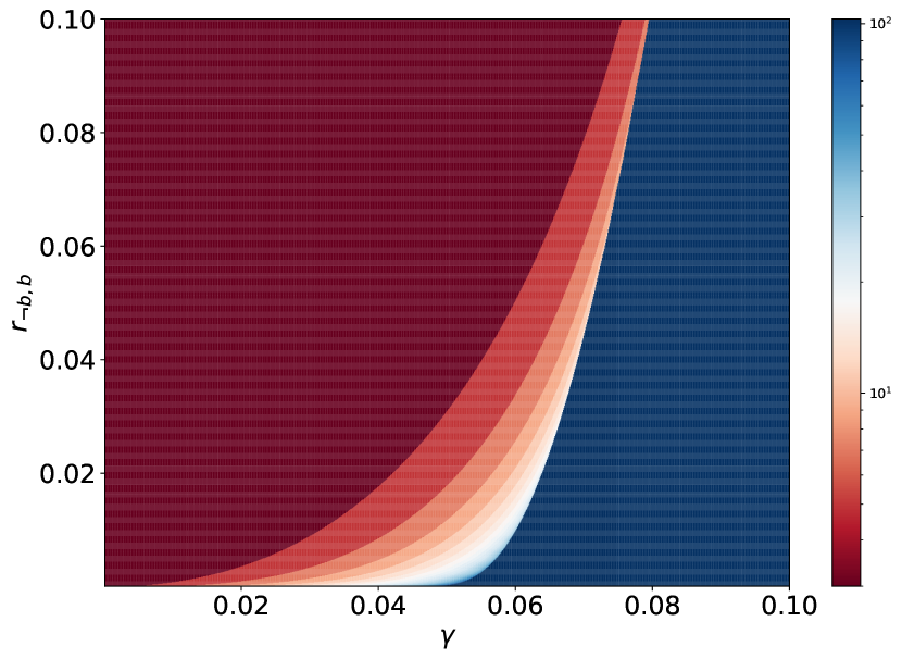
where denotes the regularized incomplete beta function. Fig. 1, shows this misidentification probability for different number of readouts in dependence of the readout error .
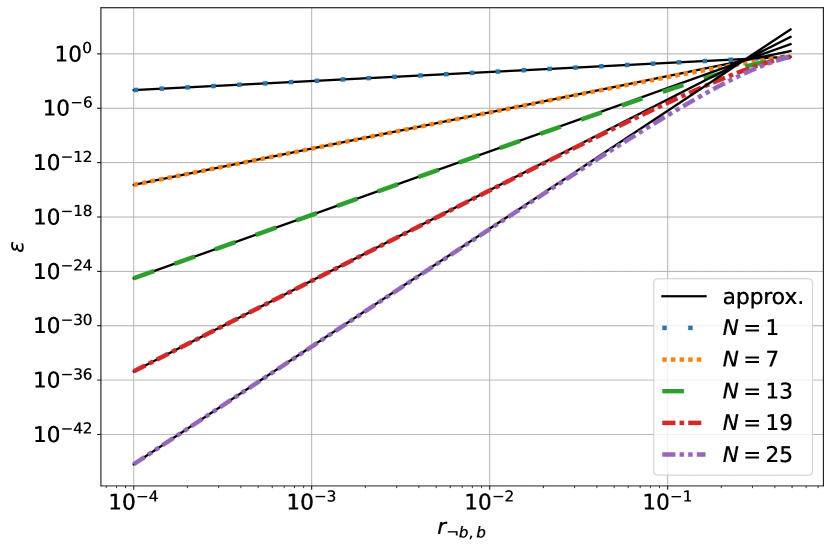
Fig. 1 shows the potential improvements of implementing this voting protocol over a large range of (base) readout errors . In particular, for realistic error rates of no more than and , the polynomial approximation
| (3) | ||||
seems to be useful for at least order of magnitude estimates.
Of course, in general we are interested in predicting the value of given a required probability of misidentification . This dependence of on within the polynomial approximation is shown in Eq. (4) and Fig. 2(a):
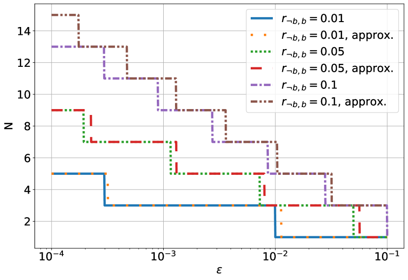
| (4) |
where denotes the Lambert function. The derivation of Eq. (4) is presented in the appendix. Since Eq. (4) is a continuous function, we have to round its value to the next higher, odd number,
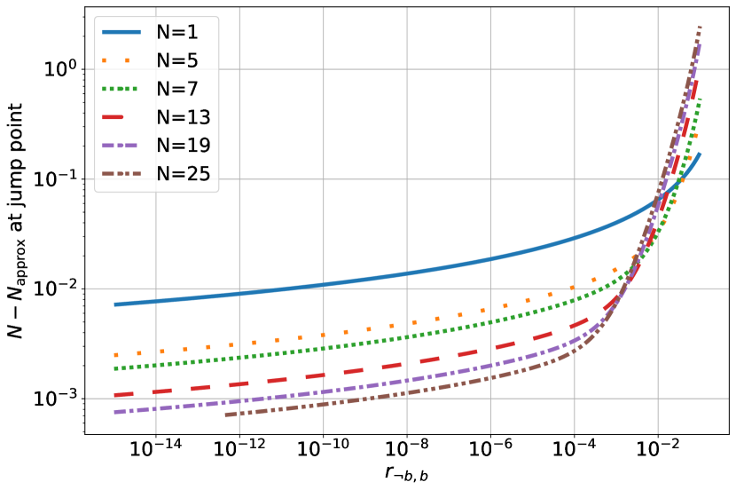
As can bee seen from Fig. 2(b), the jumps of from one odd number to the next occur at higher for the approximation in Eq. (4) than for the iterative calculation. This means that we predict slightly higher with our approximation than actually required, within a certain region of the actual jump positions. This regions get larger for larger error rates . This may be caused by the increasing deviation of the polynomial approximation from the actual incomplete, regularised beta function for higher measurement errors.
IV Mitigating projection errors in a OWQC with error-free CNOT operations
On the lowest level of a one-way quantum computation (OWQC), we are working with graph states of two qubits which are in the state
| (5) |
The qubit in the state is the target for the projective measurement in the -basis and the second qubit is used further in the quantum computation. This continuation qubit needs to be in the state which implies that a measurement of in requires an additional -gate operation. Hence, we need to reliably identify the state was projected into. Without projection errors, would be in the state after measurement, and the -gate needs to be inserted if and only if . However, with projection errors, there are probabilities of projecting into the false states which needs an application of even though is in the state, and which does not need an application of even though is in the state. Hence, we cannot identify the state of by only looking at after the measurement has taken place.
Instead, we introduce a verification register , which is initialized in the state . Before the measurement of target , we have to initialize the graph state and the verification register in the state:
| (6) |
Therefore, we have to first rotate back into the computational basis . This is achieved by the unitary . Next, we will entangle with the whole verification register by applying s between and all qubits in . Finally, we rotate all qubits ( and ) back to the measurement basis , this is achieved by applying to all qubits. The whole unitary to initialize in the desired state is thus given by
| (7) |
from which we obtain the desired state in Eq. (6). After the projective measurement of , the verification register is in the state or and we need to apply an gate if and only if the verification state is . We may now proceed with measuring each verification qubit in the -basis. Note, that if the measurement in the rotated basis is implemented via rotating the qubit into the computational basis and then performing a computational basis measurement, we can simplify the unitary of Eq. (7) and integrate it into the measurement process. For this case we simply need to apply before the computational basis measurement of , the register needs then also to be measured in the computational basis. For the measurements in there may again be projection and readout errors. If the readout can be performed separately from the projection, then the readout protocol above means we can exactly identify the state the verification qubit is in after the projective measurement. In this case, the error is purely given by the projection error. If readout cannot be separated, then we only project and measure once and receive a possibly erroneous output that combines readout and projection errors. In either case, there is an effective error rate for incorrectly identifying the state of each verification qubit, and therefore the number of readout shots in the readout-only protocol translates to the size of the verification register in the projection error setup discussed here.
V Considering CNOT errors in the verification scheme
For simplicity, we will consider pure-state preserving errors. If the -gate were error-free, then and should hold. However, if the has an error rate , then the final state of the verification qubit is
or
Either way, there is a probability that the verification qubit is in the wrong state. If we add the combined error for projection and readout, then there is a probability of that the state is verified correctly and a probability of that the state is incorrectly identified.
Hence, if we use a linear setup, that is, if we each verification qubit directly with the target qubit, then we are again in the same protocol as the projection-free readout, but we have the larger effective error rate .
If we use a -deep verification setup, that is, populating the verification register according to the following steps
-
1:
-
2:
-
-
:
then we have accumulating effects of the error to a maximum depth of .
If we model our erroneous as via the action of
in propagating the error, then we have depth errors of
If is reasonably small, say in the range, then is in the ‰ range, and so realistically, the propagated error to depth is approximately
In other words, a starting error of about with a size 64 register leads to an effective maximum error of about for which the remaining misidentification probability is according to Eq. (2). Thus, choosing a -deep verification setup with register size and , the effective error becomes
| (8) |
and the probability of misidentification becomes
| (9) |
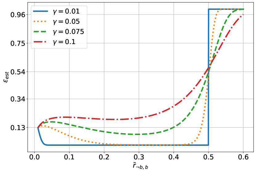
Note that, the register size and the effective error rate are now coupled according to Eq. (8). This means that for a given initial error rate and a given error , the effective error depends on the register size. In order to thus plot , will not necessarily be an integer and we will use an upper bound estimate for which avoids any floor function and allows for non-integer . This estimate is given by
| (10) |
Fig. 3 shows, the estimate of the misidentification probability in dependence of the effective error rate from Eq. (10). The function is plotted for different errors . Even for a very small error , we see that for an effective error of the misidentification probability jumps to . The protocol thus fails for effective errors , i.e., for too large register sizes. For small effective errors, a small error yields an immediate improvement. Midsize errors can result in an initial worsening before an improvement is achieved for larger register sizes. Large errors will yield no improvement at all.
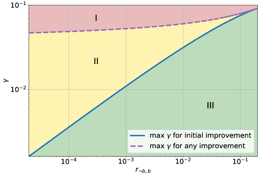
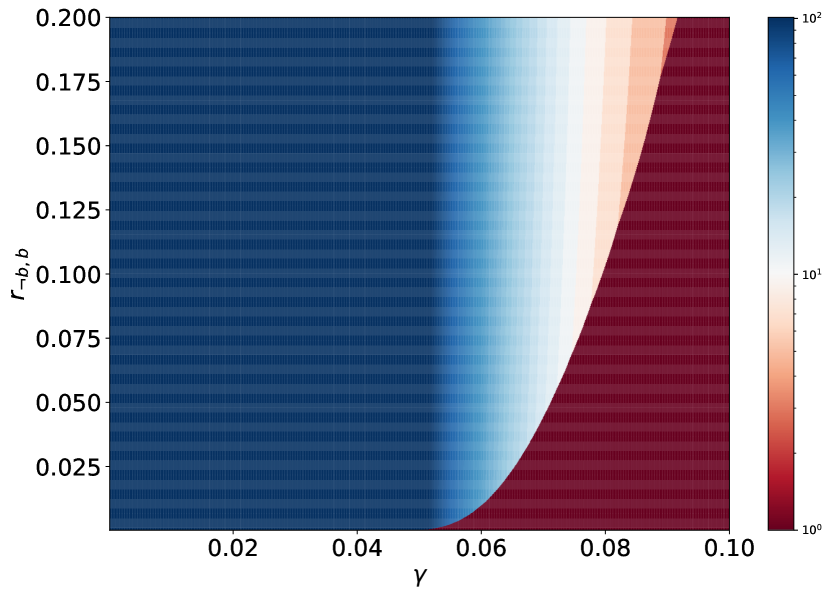
By iteratively calculating and for different values and a fixed initial error rate (c.f. Eq. (9)), we can extract the critical values that separate the three regimes (c.f. Fig. 4).
Note, that additional single-qubit gate errors during the preparation of the state in Eq. (6) from the initial graph state can also be incorporated in the error rate .
VI Simulation results
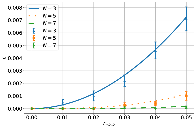
In this section we are trying to verify the theoretical prediction by applying the proposed verification scheme on the example OWQC simulation, implementing the gate acting on (c.f. Eq. (5)). For this simulation, we considered only projection errors as discussed above and no readout errors (since they can be compensated very well by reading out the state several times). The verification scheme to compensate the projection errors leads to a similar voting protocol as for the readout errors with the same predicted probability of misidentification (c.f. Eq. (2)). Overall, the simulations are in very good agreement with the theoretical predictions as shown in Fig. 5. We tested the verification scheme for different register sizes, ranging from to qubits and different projection error probabilities, ranging from to error for any qubit projection.
Additionally, we also tested our mitigation scheme in a noisy simulation with the qiskit python package, using a noise model which was derived from the ibm_nazca quantum hardware. Here, we implemented again the same OWQC from before. In order to verify the correct state of the output qubit for any angle of the OWQC, we rotated the output qubit into the computational basis by applying before measuring in this basis. The output qubit is then expected to be in the state before the measurement. Fig. 6 shows the full circuits that have been implemented in qiskit, representing the OWQC, the described measurement circuit and the described mitigation scheme.
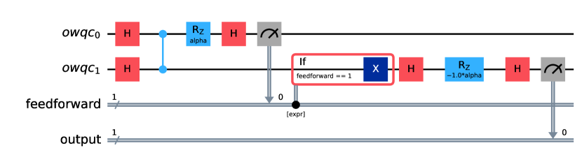
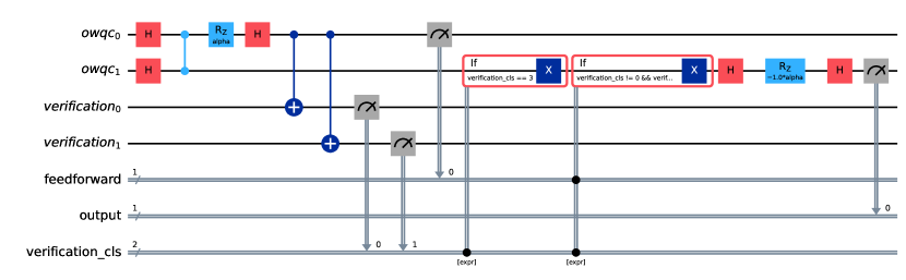
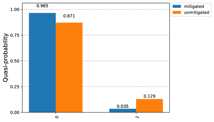
Fig. 7 shows the results of the noisy simulation for two qubits in the verification register compared to no mitigation. We see a significant improvement of the results, with the rather small overhead of two verification qubits.
VII Conclusion
We first introduced a measurement error model that, in contrast to most previous works, makes a clear distinction between errors that occur through the readout apparatus after projecting the qubit during the measurement (readout error) and the actual projection error that occurs during the projection. Note, that for cases were those two error sources are not clearly separable, we can still apply our mitigation method simply by viewing the measurement error as part of the projection error in our model. We then discussed the compensation of the readout error through a voting protocol in great detail and gave theoretical predictions on the number of consecutive readouts for given error rates and its resulting probability to misidentify the post-measurement state, which vanishes quickly with small effort in terms of the readout number. Next, we discussed the compensation of projection errors, by using a register of verification qubits that are entangled with the next to-be-measured qubit in the OWQC. Measuring the to-be-measured qubit as well as all verification qubits, allows then to apply a similar voting protocol as for the readout errors on the measurement outcomes, simply replacing the readout error with the projection error and the number of readouts with the number of measured qubits. Note that, by re-using the verification qubits after each measurement, we require only a constant number of verification qubits depending on the measurement error rates. Finally we showed in proof-of-principle simulations, including a noisy simulation representing the noise of the real ibm quantum hardware ibm_nazca, that our method works and can be used to mitigate measurement errors in real-time during a OWQC.
Acknowledgements.
We thank Ferdinand Schmidt-Kaler and his group for helpful discussions and the provided hardware data of measurement error rates. This work is funded by the European Union’s Horizon Europe Framework Programme (HORIZON) under the ERA Chair scheme with grant agreement no. 101087126 and by the Deutsche Forschungsgemeinschaft (DFG, German Research Foundation) – Project-ID 429529648 – TRR 306 QuCoLiMa (“Quantum Cooperativity of Light and Matter”). This work is supported with funds from the Ministry of Science, Research and Culture of the State of Brandenburg within the Centre for Quantum Technologies and Applications (CQTA).![[Uncaptioned image]](/html/2411.09084/assets/x10.jpg)
References
- Raussendorf and Briegel [2001] R. Raussendorf and H. J. Briegel, A one-way quantum computer, Physical Review Letters 86, 5188 (2001).
- Raussendorf et al. [2003] R. Raussendorf, D. E. Browne, and H. J. Briegel, Measurement-based quantum computation on cluster states, Physical Review A 68, 022312 (2003).
- Briegel et al. [2009] H. J. Briegel, D. E. Browne, W. Dür, R. Raussendorf, and M. Van den Nest, Measurement-based quantum computation, Nature Physics 5, 19 (2009).
- Bartolucci et al. [2021] S. Bartolucci, P. Birchall, H. Bombin, H. Cable, C. Dawson, M. Gimeno-Segovia, E. Johnston, K. Kieling, N. Nickerson, M. Pant, F. Pastawski, T. Rudolph, and C. Sparrow, Fusion-based quantum computation (2021).
- Ferguson et al. [2021] R. Ferguson, L. Dellantonio, A. A. Balushi, K. Jansen, W. Dür, and C. Muschik, Measurement-based variational quantum eigensolver, Physical Review Letters 126, 220501 (2021).
- Marqversen and Zinner [2023] F. K. Marqversen and N. T. Zinner, Applications and resource reductions in measurement-based variational quantum eigensolvers, Quantum Science and Technology 8, 045001 (2023).
- Schuster et al. [2024] S. Schuster, S. Kühn, L. Funcke, T. Hartung, M.-O. Pleinert, J. von Zanthier, and K. Jansen, Studying the phase diagram of the three-flavor schwinger model in the presence of a chemical potential with measurement- and gate-based quantum computing, Physical Review D 109, 114508 (2024).
- Qin et al. [2024] Z. Qin, X. Li, Y. Zhou, S. Zhang, R. Li, C. Du, and Z. Xiao, Applicability of measurement-based quantum computation towards physically-driven variational quantum eigensolver, New Journal of Physics 26, 073040 (2024).
- Brandhofer et al. [2024] S. Brandhofer, I. Polian, S. Barz, and D. Bhatti, Hardware-efficient preparation of graph states on near-term quantum computers (2024).
- Romero and Milburn [2024] J. Romero and G. Milburn, Photonic quantum computing (2024).
- Pino et al. [2021] J. M. Pino, J. M. Dreiling, C. Figgatt, J. P. Gaebler, S. A. Moses, M. S. Allman, C. H. Baldwin, M. Foss-Feig, D. Hayes, K. Mayer, C. Ryan-Anderson, and B. Neyenhuis, Demonstration of the trapped-ion quantum ccd computer architecture, Nature 592, 209 (2021).
- Yirka and Subaşı [2021] J. Yirka and Y. Subaşı, Qubit-efficient entanglement spectroscopy using qubit resets, Quantum 5, 535 (2021).
- Chertkov et al. [2022] E. Chertkov, J. Bohnet, D. Francois, J. Gaebler, D. Gresh, A. Hankin, K. Lee, D. Hayes, B. Neyenhuis, R. Stutz, A. C. Potter, and M. Foss-Feig, Holographic dynamics simulations with a trapped-ion quantum computer, Nature Physics 18, 1074 (2022).
- Chertkov et al. [2023] E. Chertkov, Z. Cheng, A. C. Potter, S. Gopalakrishnan, T. M. Gatterman, J. A. Gerber, K. Gilmore, D. Gresh, A. Hall, A. Hankin, M. Matheny, T. Mengle, D. Hayes, B. Neyenhuis, R. Stutz, and M. Foss-Feig, Characterizing a non-equilibrium phase transition on a quantum computer, Nature Physics 19, 1799 (2023).
- DeCross et al. [2023] M. DeCross, E. Chertkov, M. Kohagen, and M. Foss-Feig, Qubit-reuse compilation with mid-circuit measurement and reset, Physical Review X 13, 041057 (2023).
- Chan et al. [2024] A. Chan, Z. Shi, L. Dellantonio, W. Dür, and C. A. Muschik, Measurement-based infused circuits for variational quantum eigensolvers, Physical Review Letters 132, 240601 (2024).
- Bäumer et al. [2024] E. Bäumer, V. Tripathi, D. S. Wang, P. Rall, E. H. Chen, S. Majumder, A. Seif, and Z. K. Minev, Efficient long-range entanglement using dynamic circuits, PRX Quantum 5, 030339 (2024).
- Kokail et al. [2019] C. Kokail, C. Maier, R. van Bijnen, T. Brydges, M. K. Joshi, P. Jurcevic, C. A. Muschik, P. Silvi, R. Blatt, C. F. Roos, and P. Zoller, Self-verifying variational quantum simulation of lattice models, Nature 569, 355 (2019).
- Nannicini [2019] G. Nannicini, Performance of hybrid quantum-classical variational heuristics for combinatorial optimization, Physical Review E 99, 013304 (2019).
- Bravo-Prieto et al. [2020] C. Bravo-Prieto, J. Lumbreras-Zarapico, L. Tagliacozzo, and J. I. Latorre, Scaling of variational quantum circuit depth for condensed matter systems, Quantum 4, 272 (2020).
- Funcke et al. [2023] L. Funcke, T. Hartung, K. Jansen, and S. Kühn, Review on quantum computing for lattice field theory, in Proceedings of The 39th International Symposium on Lattice Field Theory — PoS(LATTICE2022), LATTICE2022 (Sissa Medialab, 2023) p. 228.
- Sobhani et al. [2024] M. Sobhani, Y. Chai, T. Hartung, and K. Jansen, Variational quantum eigensolver approach to prime factorization on ibm’s noisy intermediate scale quantum computer (2024).
- Schwägerl et al. [2024] T. Schwägerl, Y. Chai, T. Hartung, K. Jansen, and S. Kühn, Benchmarking variational quantum algorithms for combinatorial optimization in practice (2024).
- Guo et al. [2024] Y. Guo, T. Angelides, K. Jansen, and S. Kühn, Concurrent vqe for simulating excited states of the schwinger model (2024).
- Chai et al. [2024] Y. Chai, K. Jansen, S. Kühn, T. Schwägerl, and T. Stollenwerk, Structure-inspired ansatz and warm start of variational quantum algorithms for quadratic unconstrained binary optimization problems (2024).
- Di Meglio et al. [2024] A. Di Meglio, K. Jansen, I. Tavernelli, C. Alexandrou, S. Arunachalam, C. W. Bauer, K. Borras, S. Carrazza, A. Crippa, V. Croft, R. de Putter, A. Delgado, V. Dunjko, D. J. Egger, E. Fernández-Combarro, E. Fuchs, L. Funcke, D. González-Cuadra, M. Grossi, J. C. Halimeh, Z. Holmes, S. Kühn, D. Lacroix, R. Lewis, D. Lucchesi, M. L. Martinez, F. Meloni, A. Mezzacapo, S. Montangero, L. Nagano, V. R. Pascuzzi, V. Radescu, E. R. Ortega, A. Roggero, J. Schuhmacher, J. Seixas, P. Silvi, P. Spentzouris, F. Tacchino, K. Temme, K. Terashi, J. Tura, C. Tüysüz, S. Vallecorsa, U.-J. Wiese, S. Yoo, and J. Zhang, Quantum computing for high-energy physics: State of the art and challenges, PRX Quantum 5, 037001 (2024).
- Temme et al. [2017] K. Temme, S. Bravyi, and J. M. Gambetta, Error mitigation for short-depth quantum circuits, Physical Review Letters 119, 180509 (2017).
- Giurgica-Tiron et al. [2020] T. Giurgica-Tiron, Y. Hindy, R. LaRose, A. Mari, and W. J. Zeng, Digital zero noise extrapolation for quantum error mitigation, in 2020 IEEE International Conference on Quantum Computing and Engineering (QCE) (IEEE, 2020).
- Bravyi et al. [2021] S. Bravyi, S. Sheldon, A. Kandala, D. C. Mckay, and J. M. Gambetta, Mitigating measurement errors in multiqubit experiments, Physical Review A 103, 042605 (2021).
- Nation et al. [2021] P. D. Nation, H. Kang, N. Sundaresan, and J. M. Gambetta, Scalable mitigation of measurement errors on quantum computers, PRX Quantum 2, 040326 (2021).
- Funcke et al. [2021] L. Funcke, T. Hartung, K. Jansen, S. Kühn, M. Schneider, P. Stornati, and X. Wang, Towards quantum simulations in particle physics and beyond on noisy intermediate-scale quantum devices, Philosophical Transactions of the Royal Society A: Mathematical, Physical and Engineering Sciences 380, 10.1098/rsta.2021.0062 (2021).
- van den Berg et al. [2022] E. van den Berg, Z. K. Minev, and K. Temme, Model-free readout-error mitigation for quantum expectation values, Phys. Rev. A 105, 032620 (2022).
- Funcke et al. [2022] L. Funcke, T. Hartung, K. Jansen, S. Kühn, P. Stornati, and X. Wang, Measurement error mitigation in quantum computers through classical bit-flip correction, Physical Review A 105, 062404 (2022).
- van den Berg et al. [2023] E. van den Berg, Z. K. Minev, A. Kandala, and K. Temme, Probabilistic error cancellation with sparse pauli–lindblad models on noisy quantum processors, Nature Physics 19, 1116 (2023).
- Kurosawa et al. [2024] L. Kurosawa, Y. Saito, X. Lee, X. Yan, N. Xie, D. Cai, J. Shin, and N. Asai, Feed-forward probabilistic error cancellation with noisy recovery gates (2024).
- Gupta et al. [2023] R. S. Gupta, E. v. d. Berg, M. Takita, D. Riste, K. Temme, and A. Kandala, Probabilistic error cancellation for dynamic quantum circuits (2023).
- Koh et al. [2024] J. M. Koh, D. E. Koh, and J. Thompson, Readout error mitigation for mid-circuit measurements and feedforward (2024).
- Grice [2011] W. P. Grice, Arbitrarily complete bell-state measurement using only linear optical elements, Physical Review A 84, 042331 (2011).
- Ewert and van Loock [2014] F. Ewert and P. van Loock, 3/4-efficient bell measurement with passive linear optics and unentangled ancillae, Physical Review Letters 113, 140403 (2014).
- Bayerbach et al. [2023] M. J. Bayerbach, S. E. D’Aurelio, P. van Loock, and S. Barz, Bell-state measurement exceeding 50% success probability with linear optics, Science Advances 9, 10.1126/sciadv.adf4080 (2023).
- Hauser et al. [2024] N. Hauser, M. J. Bayerbach, S. E. D’Aurelio, R. Weber, M. Santandrea, S. P. Kumar, I. Dhand, and S. Barz, Boosted bell-state measurements for photonic quantum computation (2024).
Appendix A Derivation of in the polynomial approximation
The dependence of on is shown in Eq. (4) in the main text. In the following, a detailed derivation of this equation is presented.
The regularized incomplete beta function from Eq. (2), modelling the misidentification probability, can be written in the polynomial approximation shown in Eq. (3) as:
| (11) | ||||
Assuming that is an odd number, since the voting protocol would be indefinite otherwise, we can write the floor function as:
The binomial coefficient in Eq. (11) can thus be simplified as follows, using Stirling’s approximation for factorials :
This yields a compact approximation for the misidentification probability:
| (12) |
In order to invert this function for a given fixed and thus find we can use the Lambert -function. This function is defined as the inverse of ,
First, we will rewrite Eq. (12) in the form
with . Next, we apply and find the required form to use the Lambert -function
| (13) |
Note that, the argument of the Lambert has to fulfill . Since is the global minimum of . This is fulfilled for any if ,
For higher measurement errors, the polynomial approximation of the incomplete, regularized beta function deviates significantly from the exact function. In this case, other methods to extract the required for a given can be employed, e.g., iteratively calculating from while increasing .
Appendix B Detailed discussion of the regimes
As already discussed in the main text, Fig. 3 and Fig. 4 show three regimes for in dependence of the error :
-
•
Immediate improvement when we increase
-
•
Initial worsening, then improvement when we increase
-
•
No improvement at all when we increase
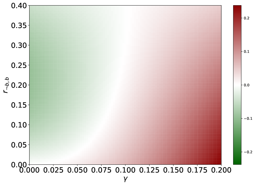
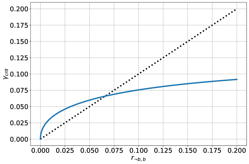
In this section, we will discuss the different regimes in more detail. Fig. 8(a) shows the change in the misidentification probability from (no verification register) and in dependence of the initial error rate and the error (c.f. Eq. (9)). In the case that is too large, needs to be sufficiently large as we will not see an initial improvement for small . The critical threshold which separates initial improvement , from initial worsening is shown in Fig. 8(b) as a function of the initial error rate . If the error is less than , we are in the region of immediate improvement and otherwise we get an initial worsening of the misidentification probability.
To answer the question, what is the with the lowest misidentification probability for a given initial error and a given error , we calculated this best iteratively from Eq. (9) and plotted it as a function of and in Fig. 9. The plot shows that for realistic errors , a bigger N is (within reasonable limits) better once the initial worsening is overcome for any initial errors . If the error is higher than , there exists a transition region depending on the initial error rate for which there is a optimal corresponding to the minimal . For errors and beyond this transition region, larger don’t yield a smaller compared to and thus yield no improvement.
Similar to the best with the smallest misidentification probability in Fig. 9, we plotted the which gives a first improvement in compared to in Fig. 10. We see that there exists a large region of immediate improvement, a small transition region where is required for improvements and then a fairly immediate jump to no improvements at all if becomes too large.