Hidden nonlinear optical susceptibilities in linear polaritonic spectra

Abstract

Linear spectra of molecular polaritons formed by $N$ molecules coupled to a microcavity photon mode are usually well described by classical linear optics, raising the question of where the expected nonlinear effects in these strongly coupled systems are. In this work, we derive a general expression for the polaritonic linear spectra that reveal previously overlooked finite-size quantum corrections due to vacuum-mediated molecular Raman processes. Using a $1/N$ expansion, we demonstrate that these nonlinearities are suppressed in typical low-Q cavities due to an emergent timescale separation in polariton dynamics yet manifest in high-Q single-mode cavities where the photon loss is comparable to the single-molecule light-matter coupling strength.

Polaritons have garnered significant attention in the last decade due to their promise to manipulate matter degrees of freedom (DOF) via coupling to a confined electromagnetic mode. They have offered a plethora of promising applications like enhanced energy transport [1, 2, 3], modification of chemical reactions  [4, 5], and room temperature lasing [6, 7]. For molecular systems, strong coupling (SC) is typically realized through the interaction of an ensemble of $N\approx 10^{6}-10^{12}$ molecules with a microcavity mode [8]. The multiple exchanges of excitation between the electromagnetic mode and the matter optical polarization (see Fig 1a) are expected to induce nonlinear optical transitions in the molecules. However, recent studies suggest that several polaritonic phenomena can be replicated using appropriately shaped lasers, causing polaritons to sometimes act just as optical filters [9]. This effect is evident in the linear response of polaritons, which is well described using classical linear optics methods, such as transfer matrices, with the molecular optical constants as the only material input [10, 11, 12, 13, 14, 15, 16]. This classical linear optics description raises a fundamental question: what happened to the nonlinearities anticipated in the SC regime? The answer to this question is also key to uncovering genuine cavity-induced effects beyond classical optics.
In this letter, we solve this apparent contradiction by obtaining a general expression for the linear response of molecular polaritons, which evidences that the classical optical description is only correct in the thermodynamic limit ($N\rightarrow\infty$) and, in fact, there is a previously overlooked hierarchy of (finite-size) $1/N$ corrections containing signatures of nonlinear molecular processes like Raman scattering mediated by quantum vacuum fluctuations of the cavity. These corrections are small due to an emergent separation of timescales in polariton dynamics and are usually excluded from the spectra due to limited resolution in the low-Q cavities typically used in experiments. They manifest in high-Q single-mode cavities where the cavity decay rate $\kappa$ becomes comparable to the single molecule coupling $\lambda$.

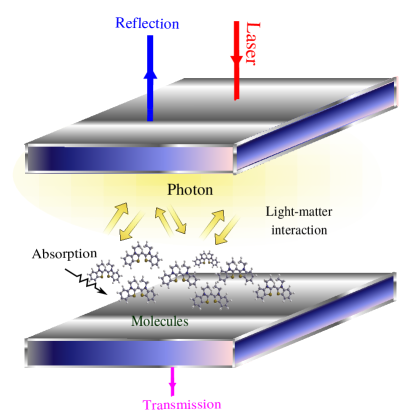
Figure 1: Strong coupling between a cavity photon and molecular optical polarization leads to multiple exchanges of excitation between light and matter. We explore the conditions under which these exchanges lead to nonlinear optical processes in the molecules, even at linear order in the incoming photon field.

Model.—We consider a photonic cavity with a single-mode of frequency $\omega_{\text{ph}}$ coupled to $N$ non-interacting molecules. Starting from a permutationally invariant initial state at zero temperature, the setup is described by a bosonic Hamiltonian at all times [Supplemental material: Sec. S1] [17, 18, 19, 20, 21, 22],

$$H = \bigg{[}\hbar\omega_{\text{ph}}a^{\dagger}a+\hbar\sum_{j}\omega_{g,j}b_{j}^{\dagger}b_{j}+\hbar\sum_{j}\omega_{e,j}B_{j}^{\dagger}B_{j}\bigg{]}+$$ (1)

$$\bigg{[}-\hbar\lambda\sum_{jj^{\prime}}\langle\varphi^{(e)}_{j^{\prime}}|\varphi^{(g)}_{j}\rangle ab_{j}B_{j^{\prime}}^{\dagger}-\text{h.c.}\bigg{]},$$

with operators $a$ that annihilates a cavity excitation (photon), and $b_{j}(B_{j^{\prime}})$ that annihilate a molecule in vibronic state $|g,\varphi^{(g)}_{j}\rangle$($|e,\varphi^{(e)}_{j^{\prime}}\rangle$); $j(j^{\prime})$ label the vibrational level in the ground (excited) electronic state. To compute linear response, we project the Hamiltonian to the first excitation manifold, where it admits a block tridiagonal representation [23]:

$$H_{1}=\begin{pmatrix}\bm{H}_{\text{ph},0}&\bm{V}_{0}&0&\dots&0&0&0\\ \bm{V}_{0}^{\dagger}&\bm{H}_{e,0}&\bm{v}_{0}&\dots&0&0&\\ 0&\bm{v}_{0}^{\dagger}&\bm{H}_{\text{ph},1}&\bm{V}_{1}&0&0&0\\ \vdots&\vdots&\vdots&\ddots&\vdots&\vdots&\vdots\\ 0&0&0&\dots&\bm{V}_{N-1}^{\dagger}&\bm{H}_{e,N-1}&\bm{v}_{N-1}\\ \vdots&\vdots&\vdots&\vdots&0&\bm{v}_{N-1}^{\dagger}&\bm{H}_{\text{ph},N}\end{pmatrix}.$$ (2)

Here $\bm{H}_{\text{ph},n}$ denotes the effective cavity single-photon Hamiltonian for the subspace where $n$ molecules have phonons in the ground state (e.g. $\bm{H}_{\text{ph},0}=(\omega_{\text{ph}}-i\kappa/2)|1_{\text{ph},0}\rangle\langle 1_{\text{ph},0}|$ for a cavity excitation with all molecules in $|g,\varphi_{0}^{(g)}\rangle$), and $\bm{H}_{e,n}$ corresponds to the photonless subspace with one molecule excited and $n$ other molecules having phonons in the ground state [24, 25]. The off-diagonal elements reveal the crucial timescale separation: couplings $\bm{V}_{n}$ drive the collective $\mathcal{O}(\lambda\sqrt{N})$ ‘Rayleigh’ transitions that conserve the number of molecules with ground state phonons, and $\bm{v}_{n}$ mediate the single-molecule $\mathcal{O}(\lambda)$ ‘Raman’ transitions that create/destroy the phonons in one of the molecules [26].

The linear spectroscopic observables of cavity-coupled systems (absorption, reflection, transmission) can be entirely expressed in terms of the photon Green’s function $D_{N}^{R}(\omega)=\langle 1_{\text{ph,0}}|\bm{G}(\omega)|1_{\text{ph,0}}\rangle$ [Supplemental material: Sec. S2], where $\bm{G}(\omega)=\frac{1}{\omega-H_{1}+i0^{+}}$. In particular, the absorption is given by  [16],

$$A(\omega) =-(\kappa/2)[\kappa|D_{N}^{R}(\omega)|^{2}+2\imaginary D_{N}^{R}(\omega)],$$ (3)

To compute $D_{N}^{R}(\omega)$, we exploit the block tridiagonal structure of $H_{1}$ and use standard techniques for matrix Green’s functions of systems with nearest neighbor couplings [see Supplemental material: Sec. S3 ] [27, 28, 29]. Rewriting the Hamiltonian $H_{1}=\begin{pmatrix}\bm{H}_{\text{ph},0}&\bm{V}_{0}\\ \bm{V}_{0}^{\dagger}&\tilde{\bm{H}}_{e,0}\end{pmatrix}$ yields

$$D_{N}^{R}(\omega)=\frac{1}{\omega-\omega_{\text{ph}}+i\kappa/2-\Sigma_{e,0}(\omega)},$$ (4)

where $\Sigma_{e,0}(\omega)=\bm{V}_{0}(\omega-\tilde{\bm{H}}_{e,0}+i\gamma/2)^{-1}\bm{V}_{0}^{\dagger}$ is the photon self-energy due to its coupling to the $\tilde{\bm{H}}_{e,0}$ block; here $\gamma\rightarrow 0$ is introduced to ensure causality of the Green’s function [30]. We next obtain an expression for $\Sigma_{e,0}(\omega)$ in terms of the bare Green’s functions and the off-diagonal light-matter couplings in Eq. 2. By iterating the technique used to obtain Eq. 4 [Supplemental material: Sec. S4], we arrive at a recursive relation where the self-energy at the $k^{\text{th}}$ step depends on the $(k+1)^{\text{th}}$ step [27, 28]:

$$\bm{\Sigma}_{e,k}= \bm{V}_{k}\big{(}\omega-\bm{H}_{e,k}+i\gamma/2-\bm{\Sigma}_{\text{ph},k+1}\big{)}^{-1}\bm{V}_{k}^{\dagger},$$ (5a)

$$\bm{\Sigma}_{\text{ph},k+1}= \bm{v}_{k}\big{(}\omega-\bm{H}_{\text{ph},k+1}+i\kappa/2-\bm{\Sigma}_{e,k+1}\big{)}^{-1}\bm{v}_{k}^{\dagger},$$ (5b)

for $0\leq k<N$. For finite $N$, the series truncates at $\bm{\Sigma}_{\text{ph},N}=\bm{v}_{N-1}\big{(}\omega-\bm{H}_{\text{ph},N}+i\kappa/2\big{)}^{-1}\bm{v}_{N-1}^{\dagger}$. Thus Eq. 4 becomes,

$$D^{R}_{N}(\omega)=\frac{1}{\omega-\omega_{\text{ph}}+i\kappa/2-\bm{V}_{0}\frac{1}{\omega-\bm{H}_{e,0}+i\gamma/2-\bm{v}_{0}^{\dagger}\frac{1}{\omega-\bm{H}_{\text{ph,1}}+i\kappa/2-\bm{V}_{1}^{\dagger}\frac{1}{\frac{\ddots}{\omega-\bm{H}_{e,N-1}+i\gamma/2-\bm{v}_{N}^{\dagger}\frac{1}{\omega-\bm{H}_{\text{ph,}N}+i\kappa/2}\bm{v}_{N}}}\bm{V}_{1}}\bm{v}_{0}}\bm{V}_{0}^{\dagger}}.$$ (6)

$1/N$ expansion.—Eq. 6 admits a $1/N$ expansion due to the aforementioned timescale separation in the polariton dynamics, $D_{N}^{R}(\omega)=\sum_{k=0}^{\infty}d_{N,k}(\omega)$ where $d_{N,k}(\omega)\propto N^{-k}$. Here, we present closed-form expressions for $d_{N,0}$ and $d_{N,1}$. For $k\geq 2$, certain non-commuting cascade processes prevent similar analytical manipulations (Supplemental material: Sec. S6), but we can still find expressions for $d_{N,k}$ correct up to $\mathcal{O}(N^{-k})$.

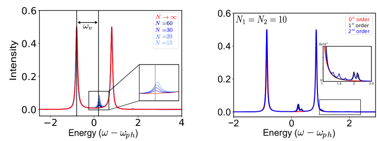
Figure 2: (a) Linear absorption spectrum of an ensemble of 3-level systems (two ground-state vibrational levels and one excited level) at zero temperature, with fixed collective coupling $\lambda\sqrt{N}$ while varying $N$. The red curve is the thermodynamic limit result $(N\rightarrow\infty)$ and is consistent with classical linear optics; it features resonances at the zeroth-order polaritons. First-order polariton sidebands show up at a vibrational frequency $\omega_{v}$ to the blue of each zeroth-order polariton and indicate Raman processes mediated by vacuum (hence, going beyond classical optics). The height of these sidebands increases as $N$ decreases due to increasing single molecule coupling $\lambda$. Parameters: $\omega_{v}=1$, $\kappa=\gamma=0.1\omega_{v}$, $\lambda\sqrt{N}=0.8\omega_{v}$, $\omega_{\text{ph}}=\omega_{\text{e,0}}$. (b) Linear absorption of an ensemble of two types of 3-level molecules with different vibrational gaps but the same electronic gap, including up to $\mathcal{O}(N^{-2})$ corrections. The red and black curves show zeroth- and first-order polaritons as in (a). The blue curve shows $\mathcal{O}(N^{-2})$ Raman corrections to the spectrum. Parameters: $\omega_{v,A}=1$, $\omega_{v,B}=1.2$, $\kappa=\gamma=0.05\omega_{v}$, $\lambda\sqrt{N}=0.6\omega_{v}$, $\omega_{\text{ph}}=\omega_{\text{e,0}}$ for both molecules.

From Eq. 6, it is easy to see that $d_{N,0}$ must have no $\bm{v}_{n}^{\dagger}$ or $\bm{v}_{n}$ terms, so,

$$d_{N,0}(\omega) =\frac{1}{\omega-\omega_{\text{ph}}+i\kappa/2-\bm{V}_{0}\bm{G}_{e,0}(\omega)\bm{V}_{0}^{\dagger}},$$ (7)

where $\bm{G}_{e,0}$ is the bare Green’s function of $\bm{H}_{e,0}$ and hence $-\bm{V}_{0}\bm{G}_{e,0}(\omega)\bm{V}_{0}^{\dagger}\equiv\frac{\omega_{\text{ph}}}{2}\chi^{(1)}(\omega)=-\text{lim}_{\gamma\to 0^{+}}N\sum_{j,j^{\prime}}|\lambda|^{2}\frac{|\langle g,\varphi_{j}^{(g)}|\mu|e,\varphi_{j}^{\prime(e)}|^{2}}{\omega-(\omega_{e,j^{\prime}}-\omega{g,j})+i\frac{\gamma}{2}}$, where $\chi^{(1)}(\omega)$ is the standard linear susceptibility of the molecular ensemble for a sample of density $N/\mathcal{V}_{\text{mol}}$ with $\mathcal{V}_{\text{mol}}$ equal to the cavity mode volume $\mathcal{V}_{\text{ph}}$, and $\mu$ as the molecular transition dipole operator. The poles of $d_{N,0}(\omega)$ will hereafter be referred to as the zeroth-order polariton frequencies. In the thermodynamic limit ($N\to\infty$ or $\lambda\to 0$ while $\lambda\sqrt{N}$ is constant), $D^{R}_{N}(\omega)\approx d_{N,0}(\omega)$; so the linear response of polaritons is compactly expressed in terms of the material linear susceptibility, a result that is consistent with classical optics [14, 16, 9].

We can proceed analogously with the $1/N$ correction [Supplemental material: Sec. S6],

$$d_{N,1}(\omega) =d_{N,0}(\omega)\cdot\bm{V}_{0}\bm{G}_{e,0}\bm{v}_{0}\big{(}\omega-\bm{H}_{\text{ph},1}+i\kappa/2-\bm{V}_{1}\bm{G}_{e,1}\bm{V}_{1}^{\dagger}\big{)}^{-1}\bm{v}_{0}^{\dagger}\bm{G}_{e,0}\bm{V}_{0}^{\dagger}\cdot d_{N,0}(\omega).$$ (8)

In the expression, we refer to the poles of $\big{(}\omega-\bm{H}_{\text{ph},1}+i\kappa/2-\bm{V}_{1}\bm{G}_{e,1}\bm{V}_{1}^{\dagger}\big{)}^{-1}$ as the first-order polariton frequencies, which are shifted from the zeroth-order polaritons by a Raman (vibrational) transition. Eq. 8 can be interpreted from right to left as a sequential Stokes-anti-Stokes Raman scattering process: (a) The photon entering the cavity through the zeroth-order polariton $d_{N,0}(\omega)$ carries out a Stokes Raman transition in one of the $N$ molecules via $\bm{v}_{0}^{\dagger}\bm{G}_{e,0}\bm{V}_{0}^{\dagger}$, (b) the leftover Stokes photon strongly couples to the $(N-1)$ remaining molecules forming first-order polaritons, where the Raman excited molecule serves as a spectator; (c) the first-order polariton now induces the reverse (anti-Stokes) Raman transition resetting all the molecules back to their electronic and vibrational ground state via $\bm{V}_{0}\bm{G}_{e,0}\bm{v}_{0}$, while releasing the photon to the zeroth-order polariton $d_{N,0}(\omega)$. Since the creation and the annihilation of the Raman phonon are cavity vacuum-mediated, these transitions are individually penalized by $1/\sqrt{N}$ and go beyond the classical optics formalism. To understand the spectroscopic fingerprints, we present an illustrative example.
Let us consider the model in Eq. 1, with each molecule having two vibrational levels in the ground state ($|g,\varphi^{(g)}_{0}\rangle$, $|g,\varphi^{(g)}_{1}\rangle$) and one excited state ($|e,\varphi^{(e)}_{0}\rangle$); this simplified model is already rich enough to illustrate the physics of interest. The vibrational gap is $\omega_{v}=\omega_{\varphi^{(g)}_{1}}-\omega_{\varphi^{(g)}_{0}}$ and the cavity is resonant with the $|g,\varphi^{(g)}_{0}\rangle\rightarrow|e,\varphi^{(e)}_{0}\rangle$ transition with frequency $\omega_{e,0}$. Fig. 2a shows the $A(\omega)$ in the thermodynamic limit and the $1/N$ corrections computed using Eq. 8. As $N$ decreases, the $1/N$ correction reveals two sidebands separated from the zeroth-order polaritons by $\omega_{v}$. These first-order polaritons have a Rabi splitting of $2\lambda\sqrt{N-1}$, and they have featured in previously reported calculations of polaritonic systems where $N$ is small [31].
The shift between the zeroth and first-order polaritons, corresponding to the energy difference of the ground state vibrational levels, provides information analogous to a Raman spectrum. A discrepancy in the Rabi splitting, $\Delta=2\lambda(\sqrt{N}-\sqrt{N-1})$, causes a blue shift in the first-order peaks (see Fig. 2a inset), due to the decrease in $\lambda\sqrt{N-1}$ as $N$ decreases while $\lambda\sqrt{N}$ remains constant. The blue-shift $\Delta$ scales as $1/\sqrt{N}$, and the peak height as $1/N$; this latter scaling can be understood from Eq. 8 since each action of $\bm{v}_{0}$ and $\bm{v}_{0}^{\dagger}$ is proportional to $N^{-1/2}$.

Even though we cannot provide an expression for $d_{N,k}$ when $k\geq 2$, the truncation of Eq. 6 at $\bm{H}_{e,k}$ gives $D^{R}_{N}(\omega)$ up to $\mathcal{O}(N^{-k})$. To best illustrate the spectroscopic implications of the $\mathcal{O}(N^{-2})$ corrections to $d_{N,0}(\omega)$, we consider a cavity coupled to $N_{A}$ and $N_{B}$ molecules of two different species. Eq. 1 can be trivially generalized to account for two sets of bosonic modes corresponding to the different molecules [32]. Each molecule is modeled as a 3-level system with different vibrational gaps, $\omega_{v,A}$ and $\omega_{v,B}$. For simplicity, let the electronic transition frequencies, $\omega_{e,\varphi^{(e)}_{0,i}}-\omega_{g,\varphi^{(g)}_{0,i}}$, is identical for both species $i=A,B$. Fig. 2b shows $A(\omega)$ for this setup. Including the second-order correction introduces sidebands shifted from the zeroth-order polaritons by $2\omega_{g,A}$, $2\omega_{g,B}$, and $\omega_{g,A}+\omega_{g,B}$ (see the three peaks appearing only in blue in the inset) due to a Raman process involving the second-order polaritons. These shifts correspond to the sum of Raman transition frequencies created in two molecules of the same or different species, in a similar way that entangled photons induce collective resonances between different molecules [33, 34].

Feynman pathways.—

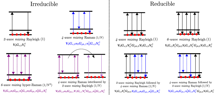
Figure 3: Cavity-mediated nonlinear molecular processes: Ladder diagrams for an ensemble of identical three-level systems with two ground-state vibrational levels and one excited state, showing second, fourth, and sixth-order transitions mediated by the cavity, classified into reducible and irreducible nonlinear susceptibilities with their correction order in the parentheses. The second-order term represents a 2-wave mixing collective Rayleigh process. The fourth-order term includes two contributions: a collective 4-wave mixing Rayleigh and a 4-wave mixing Raman. The sixth-order term has five contributions: a collective 6-wave mixing Rayleigh, two reducible terms involving 2-wave mixing Rayleigh and 4-wave mixing Raman, a 6-wave mixing Raman, and a cascade process involving two molecules with a 4-wave mixing Raman interleaved by a 2-wave mixing Rayleigh. The distinction between reducible and irreducible contributions lies in whether the excitation, after the initial $\bm{V}_{0}$ interaction with the molecular ensemble, fully returns to $\bm{H}_{\text{ph},0}$ $(\bm{G}_{\text{ph},0})$ via the $\bm{V}_{0}^{\dagger}$ interaction at any intermediate step.

For simplicity, we return to the discussion of an ensemble of identical molecules. It turns out that Eq. 6 can be rewritten as [Supplemental Material: Sec. S5],

$$D^{R}_{N}(\omega)=\frac{1}{\omega-\omega_{\text{ph}}+i\kappa/2+\sum_{l=0}^{\infty}\big{(}\frac{\omega_{\text{ph}}}{2}\big{)}^{l}\chi_{N}^{(2l+1)}(\{\omega,\omega-\omega_{\text{ph}}\}^{l},\omega)},$$ (9)

where $\sum_{l=0}^{\infty}\big{(}\frac{\omega_{\text{ph}}}{2}\big{)}^{l}\chi_{N}^{(2l+1)}(\{\omega,\omega-\omega_{\text{ph}}\}^{l},\omega)$ is the sum over all the irreducible Rayleigh and Raman nonlinear susceptibilities of the $N$-molecule ensemble ($\{\omega,\omega-\omega_{\text{ph}}\}^{l}$ denotes a string where $\omega$, $\omega-\omega_{\text{ph}}$ are repeated $l$ times). We shall now define the concept of reducible (irreducible) nonlinear susceptibilities, which describe processes that can (cannot) be decomposed into products of other bare susceptibilities, $\chi^{2l+1}_{N}(\sum_{l=1}^{2l+1}\omega_{l},\dots,\omega_{1})$ [30, 35]; as far as we aware, this concept does not exist in the literature, although similar ideas are standard in diagrammatic many-body theory [36]. The key difference between reducible and irreducible susceptibilities lies in whether, upon initial excitation of molecules via $\bm{V}_{0}^{\dagger}$, the excitation fully returns to the cavity mode via $\bm{V}_{0}$ at an intermediate step or not; see Fig. 3. It is easy to see that the expansion of the self-energy in Eq. 6 into terms of different order in light-matter coupling gives rise to irreducible diagrams only ($\bm{V}_{0}$ and $\bm{V}_{0}^{\dagger}$ act only at the beginning and end). Another interesting observation is that interpreting Eq. 9 as a geometric series gives rise to all the possible reducible and irreducible diagrams for cavity linear response.
Experimental considerations.—The spectral resolution of the polaritonic linear response is mainly determined by its cavity lifetime, $2\pi/\kappa$. Given that the peak heights correspond to the vacuum-induced nonlinearities determined by the single-molecule light-matter coupling $\lambda$, $\kappa$ must be comparable to $\lambda$ to resolve these features. This insight also helps understand why, in typical experiments with low-Q cavities, $\kappa\gg\lambda$, the truncation of the $1/N$ expansion at $d_{N,0}$ works so well. Another reason why these nonlinearities are not typically observed is due to the use of multimode cavities, given that the here-predicted first-order polariton peaks will instead blur into broad continua (the Stokes Raman photon can be emitted into any cavity mode)[37]. Thus, effective single-mode cavities are needed, which, from an experimental standpoint, translate into cavities with large free spectral ranges or with dispersionless cavities. [38, 39, 40, 41].

Summary and conclusions.—We demonstrated that while the thermodynamic limit of molecular polaritons in typical Fabry-Perot cavities, with broad linewidths, is well-captured by classical linear optics, high-Q, single-mode cavities can reveal the otherwise hidden nonlinearities expected in systems under SC. To capture these effects, we derived a general expression for the linear response of polaritons beyond the classical regime, expressed in terms of irreducible Rayleigh and Raman nonlinear susceptibilities of the molecular ensemble. By leveraging the timescale hierarchy in the polariton problem, we presented a $1/N$ expansion of this expression. While we focused on the spectroscopic aspects of the problem, we believe these higher-order coherent processes in the molecular ensemble could serve as a pathway for harnessing quantum resources such as entanglement and nontrivial photon statistics, which will be explored in future works.