An Implementation of the Finite Element Method in Hybrid Classical/Quantum Computers

Abstract

This manuscript presents the Quantum Finite Element Method (Q-FEM) developed for use in noisy intermediate-scale quantum (NISQ) computers, and employs the variational quantum linear solver (VQLS) algorithm. The proposed method leverages the classical FEM procedure to perform the unitary decomposition of the stiffness matrix and employs generator functions to design explicit quantum circuits corresponding to the unitaries. Q-FEM keeps the structure of the finite element discretization intact allowing for the use of variable element lengths and material coefficients in FEM discretization. The proposed method is tested on a steady-state heat equation discretized using linear and quadratic shape functions. Numerical verification studies demonstrate that Q-FEM is effective in converging to the correct solution for a variety of problems and model discretizations, including with different element lengths, variable coefficients, and different boundary conditions. The formalism developed herein is general and can be extended to problems with higher dimensions. However, numerical examples also demonstrate that the number of parameters for the variational ansatz scale exponentially with the number of qubits to increase the odds of convergence, and deterioration of system conditioning with problem size results in barren plateaus, and hence convergence difficulties.

Keywords: Quantum Computing; Quantum-Finite Element Method; Variational Quantum Linear Solver; Hybrid Quantum-Classical Algorithms.

1 Introduction

Quantum computing is nearing an inflection point in its evolution, as larger and distributed quantum computing devices are becoming available. These advances are beginning to allow for the development of new methodologies and algorithms for solving computational mechanics problems using quantum computers with the hope of achieving problem scales that are not accessible with classical computing. Despite significant progress in development of efficient quantum error correction algorithms, the available quantum computers remain noisy and are typically referred to as noisy intermediate-scale quantum, or NISQ computers [36]. This manuscript explores a finite element method framework for hybrid classical-NISQ computers using the variational quantum linear solver (VQLS) algorithm.

Evaluation of linearized systems of equations is a key component in most of the computational methods used for solving linear and nonlinear mechanics problems. Many of the approaches that leverage quantum computing so far consist of constructing a linear system of equations using a classical computer and evaluating this linear system by use of a quantum computer or a simulator. In their seminal work, Harrow, Hassidim, and Lloyd developed a quantum linear solver (HHL) algorithm that scales logarithmically with the linear system size and theoretically provides exponential speedup as compared to classical algorithms for systems of equations with certain properties [18]. Several improvements have been made to the original HHL algorithm since its inception (see e.g., [3, 11, 45, 48, 12])–allowing the solution of relatively large systems (e.g., $2^{17}$ equations evaluated in Ref. [33]). The HHL algorithm is suitable for fault tolerant systems and requires a level of quantum error correction that is not yet available in current NISQ devices. Quantum algorithms for iterative linear solvers offer a potential pathway to solving systems with high condition numbers [38, 39].

Bravo-Prieto et al. [7] proposed the Variational Quantum Linear Solver (VQLS) algorithm for solving linear systems in NISQ computers. VQLS is a variational quantum algorithm where the problem is evaluated via classical optimization with the associated cost function (and its derivatives) computed in a quantum computer. In VQLS, the matrix of the linear system is represented as a linear combination of unitary matrices. Quantum circuits are then prepared for each unitary matrix and used in cost function evaluations. A key difficulty in using VQLS is finding an efficient way to decompose the matrix [1]. A general methodology for symmetric real matrices as a sum of various combinations of Pauli’s spin matrices was developed in [34]. However, this approach requires solving for unknown coefficients corresponding to combinations of Pauli’s spin matrices, which are typically not readily available for general linear systems. Trahan et al. [47] recently employed this approach to solve one-dimensional time-independent Poisson’s equation and time-dependent heat and wave equations with finite element method using VQLS. The examples considered in their work consist of homogeneous material domains with constant element lengths in FEM discretization. It was concluded that the circuit depth and the number of unitaries required to decompose the matrix directly affect the time complexity of the VQLS algorithm, resulting in scalability issues for applications in practical linear systems [47]. Variational algorithms were shown to exhibit optimization convergence difficulties with increasing system size due to barren plateaus and poor representation of the solution space by the variational ansatzes [2, 9, 25, 49], subsequently attempts have been made to partially address these difficulties (see e.g., [6, 17, 24]).

Variational quantum algorithms have recently been deployed to solve solid mechanics and structural mechanics problems. Liu et al. [27] integrated variational quantum eigensolver with the finite element method to compute the fundamental natural frequency of a structure. Lu et al. [28] solved the 4th order PDE Euler-Bernoulli beam equation for general boundary conditions with a variational quantum eigensolver method. The best practices for the variational quantum eigensolver have been reviewed in Ref. [46]. The performance of discrete finite elements with VQLS was recently investigated in the context of solving one-dimensional finite element problems in Trahan et al. [47]. An alternative type of quantum computer to gate-based systems, a quantum annealing machine, has been used to solve a truss problem discretized with finite elements in a box algorithm [43]. Additionally, it has been shown that quantum annealing can achieve high solution accuracy for nonlinear elasto-plastic problems in 1D and 2D [32]. Raisuddin and De [37] developed an iterative quantum annealing algorithm for finite element problems.

This manuscript presents a new formulation of the finite element method (Q-FEM) based on the VQLS algorithm for its implementation in NISQ computers. The primary novel contribution of the proposed formulation is in its use of the finite element construction procedure to achieve a unitary representation of the global stiffness matrix. The proposed formulation allows for the automated development of efficient circuits needed for computing the VQLS cost function. The proposed formulation has been implemented in the context of steady state heat equation for elements with linear and quadratic shape functions, spatially varying properties and lengths, and subjected to natural and essential boundary conditions. The performance of the proposed approach was assessed as a function of problem characteristics (e.g., element type, problem size), as well as the variational ansatz used in problem parameterization. The proposed approach achieves significant efficiency advantage compared with generic matrix decomposition algorithms.

The remainder of this manuscript is organized as follows: Section 2 provides an overview of the VQLS algorithm, as well as the state preparation method, variational ansatzes, and cost function used in this study. Section 3 discusses the Q-FEM implementation approach, specifically the treatment of the global stiffness matrix. In Section 4, we discuss unitary and quantum circuit construction in the context of one-dimensional steady-state heat equation discretized using linear and quadratic elements. Section 5 presents the numerical verification of Q-FEM relative to ansatz selection, discretization characteristics, and boundary conditions. Section 6 provides conclusions and directions for future work.

Notation: Arbitrary vectors and matrices are represented by boldface lower and upper-case letters respectively, following the classical computational mechanics literature. The matrix-vector product of matrix $\mathbf{A}$ with a vector $\mathbf{b}$ is represented as $\mathbf{A}\mathbf{b}$. We use upper-case letters without boldface for unitary matrices (that represent circuit operations), for instance, the second order identity matrix is denoted as $I$. The quantum state vector, inner and outer products are denoted following a ‘bra-ket’ notation as described: a normalized quantum state vector is denoted as $|\cdot\rangle$, an un-normalized quantum state vector is represented with a boldface letter such as $\ket{\mathbf{a}}$, while the inner product between two quantum state vectors $|a\rangle$ and $|b\rangle$ is denoted with $\langle a|b\rangle$, and the outer product between the same states is written as $|a\rangle\langle b|$.

2 Variational Quantum Linear Solver

Variational Quantum Linear Solver (VQLS) is a quantum-classical hybrid algorithm designed for use in noisy intermediate-scale quantum (NISQ) computers [7]. VQLS solves linear matrix systems of the form $\mathbf{K}\mathbf{u}=\mathbf{f}$ requiring: (1) a process to represent the forcing vector $\mathbf{f}$ as a quantum state, (2) a method for decomposing the matrix $\mathbf{K}$ as a linear combination of $L$ unitary matrices, (3) a representation of the unitary matrices as a series of quantum gates, (4) a variational ansatz that effectively parameterizes the problem space such that a classical optimizer can be employed to find the solution, and (5) a cost function, the minimum of which corresponds to the solution.

The VQLS formulation allows for complex-valued linear systems, but we restrict our attention to real-valued systems without losing generality. Let $\mathbf{K}\in\mathbb{R}^{N\times N}$ be a full-rank, real-valued, square, consistent matrix; $\mathbf{u}\in\mathbb{R}^{N}$ and $\mathbf{f}\in\mathbb{R}^{N}$ are respectively the solution and force vectors. Consider the following quantum representations of the solution and the force vectors:

$$\mathbf{u} \rightarrow \|\mathbf{u}\||u\rangle=\|\mathbf{u}\|\sum_{i=1}^{N}\alpha_{i}|i\rangle,$$ (1)

$$\mathbf{f} \rightarrow \|\mathbf{f}\||f\rangle=\|\mathbf{f}\|\sum_{i=1}^{N}\beta_{i}|i\rangle,$$ (2)

where $|u\rangle$ and $|f\rangle$ denote the corresponding qubit state vectors, $|i\rangle$ denotes the $i^{\mathrm{th}}$ computational basis state, $\alpha_{i}$ and $\beta_{i}$ are amplitudes of the $i^{\mathrm{th}}$ computational basis state, which correspond to the $i^{\mathrm{th}}$ component of the normalized solution and force vectors. For simplicity, system size, $N$, is chosen such that $N=2^{n}$, where $n$ is the number of qubits (excluding ancilla qubits used for algorithmic purposes). The problem that the VQLS algorithm solves is as follows:

$$\mathrm{Find}\,\ket{u}\,\textrm{such that}\,\mathbf{K}\ket{u}\,\textrm{and}\,\ket{f}\hskip 2.84544pt\textrm{are collinear.}$$ (3)

The magnitude of the solution vector, $||\mathbf{u}||$, is obtained in the post-processing step after the VQLS algorithm produces a converged solution for the qubit state vector, $\ket{u}$. The magnitude can be obtained using the following expression:

$$||\mathbf{u}||=\frac{||\mathbf{f}||}{\langle f|\mathbf{K}|u\rangle},$$ (4)

where $||\mathbf{f}||$ is known, and $\langle f|\mathbf{K}|u\rangle$ is stored during the iterations in the VQLS algorithm, as discussed in Section 2.2.

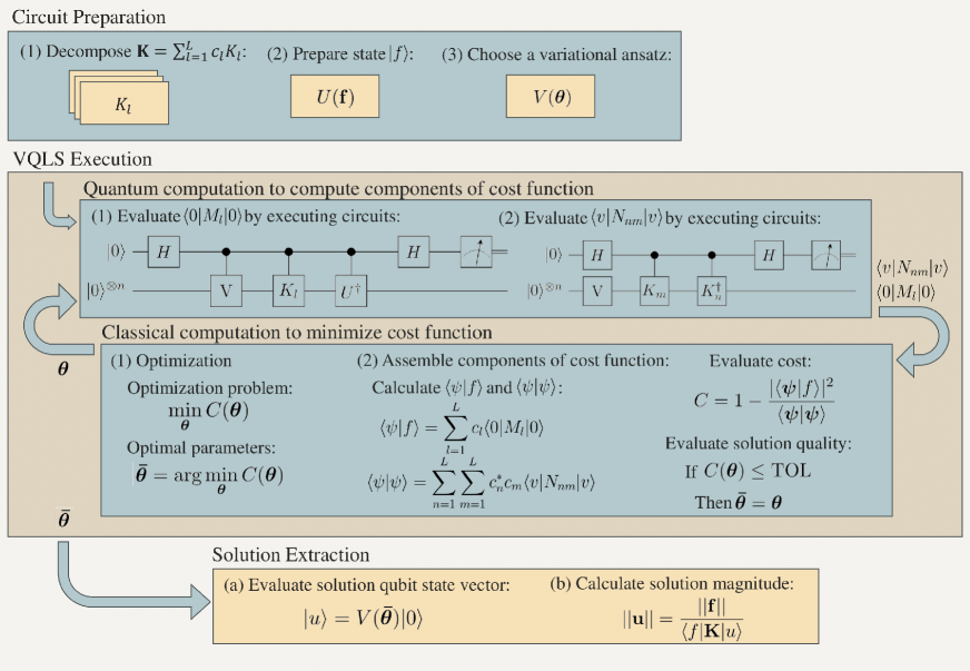
Figure 1: A flow chart for implementation of VQLS.

The overall strategy of implementing the VQLS algorithm is shown in Fig. 1 and consists of three steps: preparation of quantum circuits, execution of the VQLS optimization in a hybrid computer, and extraction of the solution. In the circuit preparation step, K is decomposed into a linear combination of unitary matrices, and a quantum circuit is prepared to represent each unitary matrix. The state vector $|f\rangle$ is prepared by implementing a state preparation algorithm $U(\textbf{f})$. Finally, the circuit representing the chosen variational ansatz is prepared. The variational ansatz defines the parametric space within which the solution of the VQLS system (i.e., $\ket{u}$) is to be searched. In the second step, a classical optimization is performed using a hybrid (quantum-classical) computer to minimize the cost function. The cost function is parameterized by the ansatz parameters, $\bm{\theta}$. Function evaluations needed to compute the cost as well as the gradients are performed in the quantum computer. The cost function is assembled in the classical computer and a search direction is determined by the classical optimization scheme. Optimization iterations continue until a specified tolerance is met. In the third step, the solution parameters $\bar{\bm{\theta}}$ are used to extract the solution unit vector from measurements of the output of the variational ansatz $|u\rangle=V(\bar{\bm{\theta}})$, as well as the solution magnitude using Eq. (4).

2.1 State preparation and variational ansatz

In order to define a cost function the minimum of which corresponds to the solution state, $\ket{u}$, two operators are defined:

$$|v\rangle = V(\bm{\theta})|0\rangle,$$ (5a)

$$|f\rangle = U(\mathbf{f})|0\rangle,$$ (5b)

in which $V(\bm{\theta})$ is the variational ansatz, and $U$ is the operator that prepares $\ket{f}$. $V$ and $U$ are unitary operators that act on a known reference state, typically taken to be a computational basis state. $\ket{0}$ is chosen as the reference state in Eqs. (5).

Mottonen et al. [31] proposed a quantum state preparation method using a circuit (i.e., $U$) with depth of $O(N)$ and made of controlled rotation gates. Closed-form analytical expressions were employed to calculate the rotation angles. This method was subsequently adapted to incorporate qubit connectivity constraint in real devices [41] and to improve efficiency [20, 35]. Further advances have been made for special cases such as symmetry-preserving [16] or sparse states [15]. Araujo et al. [4] and Bausch [5] employed an additional ancilla qubit registry to load information, which traded circuit depth for width. Optimization-based methods using direct machine pulses [29], genetic algorithms [14], or by use of an ansatz [10] have also been proposed. In this work, we adopt the method by Mottonen et al. [31] because of its general applicability.

The variational ansatz provides the parameterization of the solution space through a sequence of operations: one-qubit rotation gates applied on each qubit modify their state vector representation on the Bloch sphere by rotating around an axis in the real or imaginary plane, and two-qubit entangling gates create superposition between individual qubits and ultimately an entangled all-qubit state. These rotation and entanglement gates are applied in alternating layers. The elements of the parameter vector, $\bm{\theta}$, are the rotation angles for each rotation gate. The variational ansatz is chosen based on the problem characteristics as well as the quantum hardware employed. An ansatz that uses gates native to a particular quantum hardware is termed a hardware-efficient ansatz [7], which reduces the gate overhead and avoids additional compiling by hardware controls. The structure of the ansatz itself could be parameterized as explored in [23], whereas a “fixed-structure ansatz” employs a constant gate structure–only varying rotation parameters $\bm{\theta}$ [7]. In this work, we tested several fixed-structure anstazes.

2.2 Cost function

Consider the vector $\ket{\bm{\psi}}$ such that $\ket{\bm{\psi}}(\bm{\theta}):=\mathbf{K}\ket{v}$. A straightforward and intuitive cost function for solving the VQLS problem in Eq. (3) is [7]:

$$C_{p}=\langle\bm{\psi}|\mathbf{P}|\bm{\psi}\rangle,$$ (6)

in which, $\mathbf{P}$ is a projection operator defined as:

$$\mathbf{P}=I-|f\rangle\langle f|,$$ (7)

where $I$ is the identity matrix. By this definition of the cost function, it is easy to see that when $\ket{\bm{\psi}}$ is normal to $\ket{f}$, the value of the cost function is $\innerproduct{\bm{\psi}}{\bm{\psi}}$, whereas the cost function vanishes when the two vectors are collinear. Normalizing the cost function yields:

$$\hat{C}_{p}=1-\frac{|\langle\bm{\psi}|f\rangle|^{2}}{\langle\bm{\psi}|\bm{\psi}\rangle}.$$ (8)

$\hat{C}_{p}$ is defined in terms of the global qubit state. Barren plateaus are observed for such global cost functions in Refs. [9, 21], which motivated the proposal of local cost functions where states or operators are compared with respect to each individual qubit, rather than a global state. Local cost functions exhibit polynomially vanishing gradients, given the ansatz layer depth is $\mathcal{O}(\log(n))$, compared to exponentially vanishing gradients for global cost functions [9], which may yield better convergence, especially for large problem sizes. However, in this work, we use the global cost function as the ansatz layer depth required to resolve the solution space in numerical examples is $\mathcal{O}(n^{p})$ (with $0<p<2$), as discussed later in Section 5.3, so using a local cost function may not yield much benefit in convergence.

The optimization problem to identify the solution to Eq. (3) is then stated as:

$$\bar{\bm{\theta}}=\operatorname*{arg\,min}_{\bm{\theta}\in\bm{\Theta}\subset\mathbb{R}^{P}}\hat{C}_{p}\left(\bm{\theta}\right),$$ (9)

such that the best approximation to $\ket{u}$ is obtained as $V(\bar{\bm{\theta}})\ket{0}$. $\ket{u}$ is exact if $\hat{C}_{p}\left(\bar{\bm{\theta}}\right)=0$.

The cost function is primarily computed in a quantum computer. In order to facilitate this, the matrix, $\mathbf{K}$, is decomposed into $L$ unitary matrices:

$$\mathbf{K}=\sum_{l=1}^{L}c_{l}K_{l}.$$ (10)

Using Eqs. (5) and (10), the components of the cost function are expressed as:

$$|\langle\bm{\psi}|f\rangle|^{2} = \sum_{n=1}^{L}\sum_{m=1}^{L}c_{n}^{*}c_{m}\langle 0|M_{m}|0\rangle\langle 0|M^{\dagger}_{n}|0\rangle,$$ (11a)

$$\langle\bm{\psi}|\bm{\psi}\rangle = \sum_{n=1}^{L}\sum_{m=1}^{L}c_{n}^{*}c_{m}\langle v|N_{nm}|v\rangle,$$ (11b)

where the unitary operators are defined as $M_{l}=U^{\dagger}K_{l}V$ and $N_{nm}=K^{\dagger}_{n}K_{m}$ and are real valued in our implementation. Consequently, $\langle 0|M_{l}|0\rangle$ is real, and $\langle 0|M_{l}|0\rangle=(\langle 0|M_{l}|0\rangle)^{*}=\langle 0|M^{\dagger}_{l}|0\rangle$. This symmetry is leveraged in the computation of Eq. (11a). The cost function computation then consists of (1) preparation of $L(L-1)$ (in case of symmetry, $L(L-1)/2$) circuits associated with $N_{nm}$ and $L$ circuits associated with $M_{l}$, (2) employing the Hadamard test to compute $\innerproduct{0}{M_{l}|0}$ and $\langle v|N_{nm}|v\rangle$ in the quantum computer, and (3) evaluation of the multiplication and sum operations in Eqs. (11) using a classical computer.

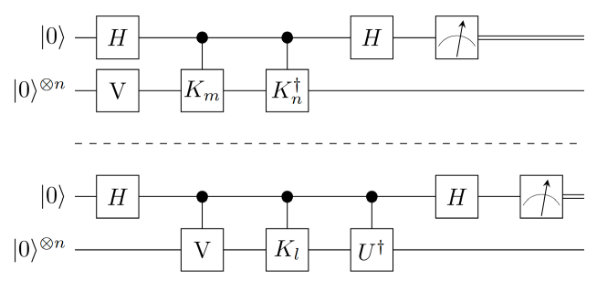
Figure 2: The Hadamard test to compute the components of the cost function. The top circuit outputs $\langle\bm{\psi}|\bm{\psi}\rangle$ in $L(L-1)/2$ runs. The bottom circuit outputs $\langle\bm{\psi}|f\rangle$ in $L$ runs.

The implementation of the Hadamard test [13] for the components of the cost function is shown in Figure 2. The Hadamard test determines the expected real component of a unitary operation on a state (e.g., $\langle v|N_{nm}|v\rangle$) by measurement of an ancillary qubit. This is done by subtracting the probability of a zero state and one state on the ancilla, $P(0)-P(1)$. It is constructed by applying a Hadamard gate on the ancilla, controlling the unitary operation on the main register onto the ancilla, and applying another Hadamard gate on the ancilla. The uncontrolled $V(\bm{\theta})$ gate operating on the main register (Fig. 2) prepares the state $|v\rangle$.

3 FEM Implementation based on VQLS

In this section, we describe the proposed approach to implement the finite element method (FEM) using VQLS. In the remainder of the manuscript, we refer to the proposed formulation as quantum finite element method (Q-FEM). We first discuss the general methodology and apply it to a one-dimensional steady-state heat equation.

Let $\mathcal{L}$ be a linear operator acting on an unknown field, $u$ that satisfies the expression $\mathcal{L}(u)=f$, where $f$ is a known field (i.e., forcing function). Considering the classical continuity and regularity requirements, the boundary and initial conditions, and using the FEM procedure results in a linear system of the form: $\mathbf{K}\mathbf{u}=\mathbf{f}$. The structure and properties of the stiffness matrix are dictated by the form of the linear operator, finite element discretization, shape functions used, node numbering, the method used for enforcing the boundary conditions, and in unstable problems, the stabilization terms. A critical consideration that differentiates quantum computer (QC) implementation of FEM (e.g., from finite difference method) is that FEM allows for unstructured grids that facilitate representation of complex geometries. The standard construction procedure for the global stiffness matrix and force vectors is the assembly operation:

$$\mathbf{K}=\bigwedge_{e=1}^{n_{\mathrm{el}}}\mathbf{k}^{e},$$ (12)

in which, $\mathbf{k}^{e}$ is the element stiffness matrix. The assembly operation performs mapping of the element degrees of freedom onto the global degrees of freedom. Element matrices associated with boundaries are treated in a slightly different manner. For simplicity, we ignore these complications in the current discussion and provide relevant details in the application of the approach to the heat equation.

An alternative construction procedure is based on the direct stiffness method [26]. This approach consists of constructing ‘global’ element stiffness matrices first, and summing the global element stiffness matrices to compute the stiffness matrix:

$$\mathbf{K}=\displaystyle\sum_{e=1}^{n_{\mathrm{el}}}\mathbf{K}^{e}.$$ (13)

The difference between the standard assembly and the direct stiffness assembly is that the latter delineates the local-to-global mapping from the addition operations. Each global element stiffness matrix, $\mathbf{K}^{e}$, has the same size as the stiffness matrix. Equation 13 also implies that global element stiffness matrices are generated for each element. This condition will be relaxed using a concept of ‘unique element’ as discussed in Section 4.3. In this study, we employ the direct stiffness assembly approach, which allows a more straightforward QC implementation as mapping and summation operations are separated.

Representing each global element matrix as a linear combination of unitary matrices, the global stiffness matrix is expressed as:

$$\mathbf{K}=\displaystyle\sum_{e=1}^{n_{\mathrm{el}}}\sum_{m=1}^{M^{e}}c^{e}_{m}K^{e}_{m}.$$ (14)

where $c^{e}_{m}$ and $K^{e}_{m}$ denote the weights and the unitary matrices, respectively. Noting that ${M^{e}}$ is bounded by a small number defined by the structure of the element stiffness matrix, and that the number of elements in a finite element discretization scale with the number of degrees of freedom, the number of unitary matrices is of $\mathcal{O}(N)$. For fully or partially structured grids, this linear scaling could be broken and a constant set of unitaries could be sufficient. We note that, if the number of unitary matrices is reduced in case of structured grids, the depth of the resulting circuits linearly increase with $N$. This effect is demonstrated in Section 4.3.

Implementation of the QFEM approach therefore requires (1) identifying the unitary matrices that efficiently represent the global element matrices (i.e., minimize $M^{e}$) and (2)  developing the quantum circuits for each unitary matrix. The proposed construction procedure is outlined as follows: consider a library of circuits, $\mathcal{C}_{I}$, parameterized by an index set, $I:=\{i,j,\ldots\}$; this library is chosen such that it contains the corresponding circuit representation of each unitary matrix, $K^{e}_{m}$. We then define a generator function, $\mathcal{G}(e,m)$, that maps each unitary matrix with its corresponding circuit in the library. In the next section, we provide examples of the circuit construction in the context of the steady-state heat equation.

In this study, the global force vector is constructed classically first and represented as a quantum state vector as discussed in Section 2.2.

4 Application to the Steady-State Heat Equation

We first consider the 1-d steady-state heat equation with homogeneous Dirichlet boundary conditions. The strong form governing equation is given as follows:

$$c(x)\frac{d^{2}u(x)}{dx^{2}}+b(x)=0,\quad\forall x\in[x_{1},x_{2}],$$ (15)

$$u(x_{1})=0,\quad u(x_{2})=0.$$

For a given discretization of the domain, we show in the successive sections, how to generate the unitaries and the corresponding quantum circuits, that represent the stiffness matrix, for both linear and quadratic elements. The required changes in the unitaries and the quantum circuit to model the Neumann boundary condition and the non-zero Dirichlet boundary condition are discussed in a later subsection.

4.1 Linear elements

The domain is discretized with $n_{\mathrm{el}}$ linear elements, and the total number of nodes is $n_{\mathrm{el}}+1$. For simplicity, the total number of internal nodes is chosen such that $N=2^{n}$, where $n$ is the number of qubits in the quantum circuit. The total number of nodes is $N+2$, accounting for the boundary nodes. Hence, for an $n$-qubit system, $n_{\mathrm{el}}$ is equal to $2^{n}+1$. The element numbering is selected such that $\mathbf{K}^{0}$ and $\mathbf{K}^{n_{\mathrm{el}}-1}$ are global-element matrices for boundary elements, and $\mathbf{K}^{e}$ for $e\in[1,n_{\mathrm{el}}-2]$ are internal element matrices.

The global-element stiffness matrices for the boundary elements $\mathbf{K}^{0}$ and $\mathbf{K}^{n_{\mathrm{el}}-1}$, as well as for an internal element $\mathbf{K}^{e}$ are:

$$\mathbf{K}^{0}=\frac{c^{0}}{h^{0}}\begin{bmatrix}1&0&\cdots&0\\ 0&0&\cdots&0\\ \vdots&\vdots&\ddots&\vdots\\ 0&0&\cdots&0\end{bmatrix}_{N\crossproduct N},\quad\mathbf{K}^{n_{\mathrm{el}}-1}=\frac{c^{n_{\mathrm{el}}-1}}{h^{n_{\mathrm{el}}-1}}\begin{bmatrix}0&\cdots&0&0\\ \vdots&\ddots&\vdots&\vdots\\ 0&\cdots&0&0\\ 0&\cdots&0&1\end{bmatrix}_{N\crossproduct N},$$ (16)

$$\mathbf{K}^{e}=\frac{c^{e}}{h^{e}}\begin{bmatrix}\{0\}_{e-1\crossproduct e-1}&\{0\}_{e-1\crossproduct 1}&\cdots&\cdots&\cdots&\{0\}_{e-1\crossproduct 1}\\ \{0\}_{1\crossproduct e-1}&1&-1&0&\cdots&0\\ \{0\}_{1\crossproduct e-1}&-1&1&0&\cdots&0\\ \{0\}_{1\crossproduct e-1}&0&0&0&\cdots&0\\ \vdots&\vdots&\vdots&\vdots&\ddots&\vdots\\ \{0\}_{1\crossproduct e-1}&0&0&0&\cdots&0\end{bmatrix}_{N\crossproduct N},$$

where $h^{e}$ denotes element length, and $c^{e}$ is the diffusivity in element $e$. The global-element matrices are represented as a linear combination of unitary matrices as:

$$\mathbf{K}^{e}=\displaystyle\frac{c^{e}}{h^{e}}\begin{cases}\displaystyle\frac{1}{2}\left(I-I_{e}^{-1}\right)&e\in\{0,n_{\mathrm{el}}-1\}\\ \left(I-X_{e}\right)&e\in[1,n_{\mathrm{el}}-2]\end{cases}$$ (17)

where $I$ is the identity matrix, $I_{e}^{-1}$ and $X_{e}$ are unitaries corresponding to the boundary and internal elements, respectively. One can obtain the linear combination of unitaries that represents the stiffness matrix as:

$$\mathbf{K}=\left(\frac{c^{0}}{2h^{0}}+\sum_{e=1}^{n_{\mathrm{el}}-2}\frac{c^{e}}{h^{e}}+\frac{c^{n_{\mathrm{el}}-1}}{2h^{n_{\mathrm{el}}-1}}\right)I-\frac{c^{0}}{2h^{0}}I_{0}^{-1}-\sum_{e=1}^{n_{\mathrm{el}}-2}\frac{c^{e}}{h^{e}}X_{e}-\frac{c^{n_{\mathrm{el}}-1}}{2h^{n_{\mathrm{el}}-1}}I_{n_{\mathrm{el}}-1}^{-1}.$$ (18)

Equation (18) indicates that the global stiffness matrix is represented using $n_{\mathrm{el}}+1=2^{n}+2$ unitary matrices. Under certain conditions, it is possible to reduce the number of unitary matrices substantially, and these conditions are discussed in Section 4.3.

4.1.1 Circuit generation

We first proceed with the description of the most general case, where no unitary reduction is possible. The unitary matrices associated with the boundary elements and an internal element $e$ are:

$$I_{0}^{-1}=\frac{c^{0}}{2h^{0}}\begin{bmatrix}-1&0&0&\cdots&0\\ 0&1&0&\cdots&0\\ 0&0&1&&0\\ \vdots&\vdots&&\ddots&\\ 0&0&0&&1\end{bmatrix}_{N\crossproduct N},\quad I_{n_{\mathrm{el}}-1}^{-1}=\frac{c^{n_{\mathrm{el}}-1}}{2h^{n_{\mathrm{el}}-1}}\begin{bmatrix}1&0&0&\cdots&0\\ 0&1&0&\cdots&0\\ 0&0&\ddots&\ddots&\vdots\\ \vdots&\vdots&\ddots&1&0\\ 0&0&\cdots&0&-1\end{bmatrix}_{N\crossproduct N},$$ (19)

$$X_{e}=\frac{c^{e}}{h^{e}}\begin{bmatrix}\{I\}_{e-1\crossproduct e-1}&\{0\}_{e-1\crossproduct 1}&\cdots&\cdots&\cdots&\{0\}_{e-1\crossproduct 1}\\ \{0\}_{1\crossproduct e-1}&0&1&0&\cdots&0\\ \{0\}_{1\crossproduct e-1}&1&0&0&\cdots&0\\ \{0\}_{1\crossproduct e-1}&0&0&1&\cdots&0\\ \vdots&\vdots&\vdots&\vdots&\ddots&\\ \{0\}_{1\crossproduct e-1}&0&0&0&&1\end{bmatrix}_{N\crossproduct N}.$$

The quantum circuits for the unitaries of internal elements ${X}_{e}$ are generated based on three types of circuits, which are as follows:

• Based on Pauli $X$ gates with control operations: $X_{i}^{0}$.

• Based on swap gates with control operations: $X_{i}^{1}$.

• Based on those generated by gray code: $X_{i}^{2}\ldots X_{i}^{n-1}$.

The relationship between these circuit types and the internal element unitary, ${X}_{e}$, is established using the following generator function:

$$X_{e}=X_{2^{j}+i\>2^{j+1}}=X_{i}^{j};\hskip 8.5359pti\in\{0,1,\ldots,2^{n-j-1}-1\};\hskip 8.5359ptj\in\{0,1,\ldots,n-1\};$$ (20)

where $e=2^{j}+i\>2^{j+1}$ provides the mapping between the element and the circuit type. The index $i$ denotes the control operations on these circuits, while $j$ denotes the number of qubits $(j+1)$ that are flipped in the corresponding unitary matrix.

The three circuit types for an $n$ qubit system are obtained as follows:

1. $X^{0}_{i}$ circuit: in the unitary matrix corresponding to this circuit, one of the qubits is flipped. This is achieved by applying Pauli $X$ gate to the $q_{0}$ (first) qubit controlled by the remaining qubits. The subscript $i$ denotes a particular control operation out of $2^{n-1}$ possibilities on the remaining $n-1$ qubits, as each control qubit can be either open-controlled or close-controlled. In particular, $i$ denotes the control operation corresponding to the $(i+1)^{\mathrm{th}}$ basis state for the control qubits. This is illustrated in Fig. 3a-d for the 3-qubit example. For $n=3$, $i=0$ denotes open control operations on the control qubits based on the first basis state $\ket{00}$, while $i=1$ denotes open and closed control operations on $q_{2}$ and $q_{1}$ qubits respectively, based on the second basis state $|01\rangle$.

2. $X^{1}_{i}$ circuit: the number of qubits flipped in the unitary matrix corresponding to this circuit is $2$. To obtain the corresponding unitary matrix, a swap gate is applied between the first two qubits $q_{0}$ and $q_{1}$. $i$ denotes a particular control operation out of $2^{n-2}$ possibilities on the remaining $n-2$ qubits. As deduced for $X^{0}_{i}$ circuit, the control operation $i$ corresponds to the $(i+1)^{\mathrm{th}}$ basis state for the remaining $n-2$ qubits. Corresponding circuits for the 3-qubit case are shown in Fig. 3e-f. For $n=3$, $i=0$ denotes open control operation on the control qubits based on the first basis state $\ket{0}$, while $i=1$ denotes closed control operation on $q_{3}$ based on the second basis state $|1\rangle$. Naturally, the three layers of operations could be replaced by a single controlled swap gate as well, shown in Fig. 3g for $X^{1}_{0}$ circuit.

3. $X_{i}^{j}$ circuits with $j\in\{2,3,\cdots,n-1\}$: the number of flipped qubits in the unitary matrix corresponding to this circuit is $j+1$. The depth of the circuit is $2j+1$, and each layer has controlled Pauli $X$ gates. The number of pure control qubits (where no $X$ gate is applied) is $n-j-1$, which are controlled based on their $(i+1)^{\mathrm{th}}$ basis state. Based on the gray code, a series of controlled $X$ circuits are designed to generate the circuit corresponding to the transformation in the unitary matrix. For example, a basis state $|{\color[rgb]{1,0,0}1\cdots 0}0111\cdots 1\rangle$ transforms to $|{\color[rgb]{1,0,0}1\cdots 0}1000\cdots 0\rangle$ state and vice-versa, with the qubits highlighted in red are pure control qubits and the qubits in black are the ones that are flipped. A series of controlled $X$ circuits to obtain the specific unitary matrix are demonstrated for two examples.

   First, given a $5$-qubit system, a series of operations for $X^{3}_{0}$ circuit (shown in Fig. 3h) are listed: firstly a $|{\color[rgb]{1,0,0}0}0111\rangle$ state is transformed to $|{\color[rgb]{1,0,0}0}1111\rangle$, then from $|{\color[rgb]{1,0,0}0}1111\rangle$ to $|{\color[rgb]{1,0,0}0}1011\rangle$, and then from $|{\color[rgb]{1,0,0}0}1011\rangle$ to $|{\color[rgb]{1,0,0}0}1001\rangle$ and finally from $|{\color[rgb]{1,0,0}0}1001\rangle$ to $|{\color[rgb]{1,0,0}0}1000\rangle$. Then reverse transformations in the opposite order are done starting from $|{\color[rgb]{1,0,0}0}1001\rangle$ to $|{\color[rgb]{1,0,0}0}1011\rangle$ (leaving the penultimate one) till the first state to begin with is obtained. These operations are done using controlled Pauli $X$ gates, with the control operations in non-pure control qubits changing accordingly.

   Second, for a $5$-qubit system and $X^{2}_{1}$ circuit shown in Fig. 3i, these operations are listed: firstly a $|{\color[rgb]{1,0,0}01}011\rangle$ state is transformed to $|{\color[rgb]{1,0,0}01}111\rangle$, then from $|{\color[rgb]{1,0,0}01}111\rangle$ to $|{\color[rgb]{1,0,0}01}101\rangle$, and finally from $|{\color[rgb]{1,0,0}01}101\rangle$ to $|{\color[rgb]{1,0,0}01}100\rangle$. Then reverse transformations in the opposite order are performed starting from $|{\color[rgb]{1,0,0}01}101\rangle$ state to $|{\color[rgb]{1,0,0}01}111\rangle$ state (leaving the penultimate one) till the first state to begin with is obtained. All of these operations are performed using controlled Pauli $X$ gates.

(a) ${X}_{1}=X_{0}^{0}$

(b) ${X}_{3}=X_{1}^{0}$

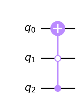
(c) ${X}_{5}=X_{2}^{0}$

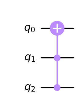
(d) ${X}_{7}=X_{3}^{0}$

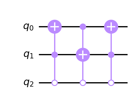
(e) ${X}_{2}=X_{0}^{1}$

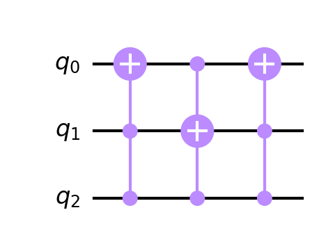
(f) ${X}_{6}=X_{1}^{1}$

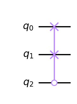
(g) ${X}_{2}=X_{0}^{1}$

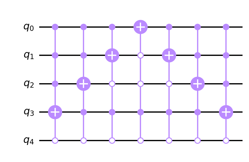
(h) ${X}_{8}=X_{0}^{3}$

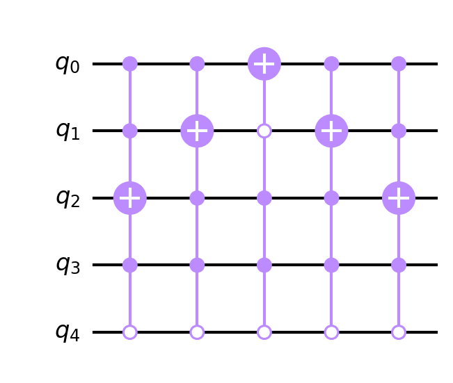
(i) ${X}_{12}=X_{1}^{2}$

Figure 3: Examples of quantum circuits for unitaries corresponding to internal elements for a 3-qubit system (a)-(g) and 5-qubit system (h)-(i).

The quantum circuits for the unitaries corresponding to boundary elements are explained below:

1. The $I_{0}^{-1}$ circuit is a controlled $Ry$ rotation gate with $\theta=2\pi$ as a parameter on $q_{0}$ qubit and open control operations on remaining $n-1$ qubits. This is followed by a controlled $Z$ gate with closed control on the $q_{0}$ qubit and open controls on the remaining $n-1$ qubits.

2. The $I_{n_{\mathrm{el}}-1}^{-1}$ circuit is a controlled $Z$ gate with closed control operations on the $n$ qubits.

The quantum circuits for the unitaries corresponding to boundary elements are shown in Fig. 4 for a 3-qubit system.

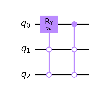
(a) ${I}_{0}^{-1}$

(b) ${I}_{8}^{-1}$

Figure 4: Examples of quantum circuits for unitaries corresponding to boundary elements for a 3-qubit system.

4.2 Quadratic elements

Figure 5 shows the discretization of the problem domain using quadratic elements. Considering an $n$ qubit register, the total number of internal nodes is $\tilde{N}=2^{n}-1$. The number of elements is $n_{\mathrm{el}}=(\tilde{N}+1)/2=2^{n-1}$. Let us denote the position coordinate of node $A$ as $x_{A}$, and the internal nodes in the domain are such that $1\leq A\leq\tilde{N}$, and the position coordinates of boundary nodes are $x_{0}$ and $x_{\tilde{N}+1}$. The length of an element is given by $h_{e}=x_{2e+2}-x_{2e}$. It is worthy of note that the size of a state vector that can be represented in the quantum computer is $N=2^{n}=\tilde{N}+1$. To accommodate this, an auxiliary degree of freedom is added to the system, and hence the size of the global stiffness matrix and global force vector are $N\times N$ and $N$, respectively.

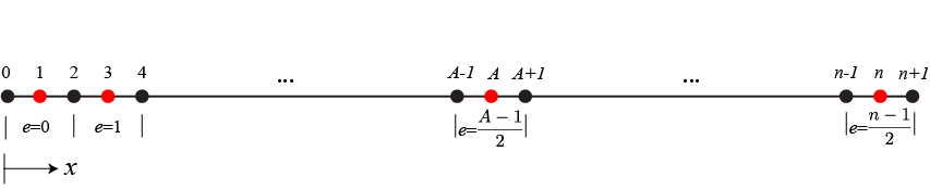
Figure 5: The discretization of the domain into quadratic elements.

As per the discretization of the problem domain shown in Fig. 5, the boundary elements correspond to $e=0$ and $e={n_{\mathrm{el}}-1}$, while the internal elements are $e\in[1,n_{\mathrm{el}}-2]$. For an $n$-qubit system, the global-element matrices for boundary elements $\mathbf{K}^{0}$ and $\mathbf{K}^{n_{\mathrm{el}}-1}$ are:

$$\mathbf{K}^{0}=\frac{c^{0}}{3h^{0}}\begin{bmatrix}16&-8&0&0&\cdots&0\\ -8&7&0&0&\cdots&0\\ 0&0&0&0&\cdots&0\\ 0&0&0&0&\cdots&0\\ \vdots&\vdots&\vdots&\vdots&\ddots&\vdots\\ 0&0&0&0&\cdots&0\end{bmatrix},\mathbf{K}^{n_{\mathrm{el}}-1}=\frac{c^{n_{\mathrm{el}}-1}}{3h^{n_{\mathrm{el}}-1}}\>\begin{bmatrix}0&\cdots&0&0&0&0\\ \vdots&\ddots&\vdots&\vdots&\vdots&0\\ 0&\cdots&0&0&0&0\\ 0&\cdots&0&0&0&0\\ 0&\cdots&0&0&16&-8\\ 0&\cdots&0&0&-8&7\end{bmatrix},$$ (21)

and for an arbitrary internal element $\mathbf{K}^{e}$ is:

$$\mathbf{K}^{e}=\frac{c^{e}}{3h^{e}}\begin{bmatrix}\{0\}_{2e-1\times 2e-1}&\{0\}_{2e-1\times 1}&\cdots&\cdots&\cdots&\cdots&\{0\}_{2e-1\times 1}\\ \{0\}_{1\times 2e-1}&7&-8&1&0&\cdots&0\\ \{0\}_{1\times 2e-1}&-8&16&-8&0&\cdots&0\\ \{0\}_{1\times 2e-1}&1&-8&7&0&\cdots&0\\ \{0\}_{1\times 2e-1}&0&0&0&0&\cdots&0\\ \vdots&\vdots&\vdots&\vdots&\vdots&\ddots&\vdots\\ \{0\}_{1\times 2e-1}&0&0&0&0&\cdots&0\end{bmatrix}_{N\crossproduct N}.$$ (22)

The global-element matrices for quadratic elements are expressed as a linear combination of unitary matrices as follows

$$\mathbf{K}^{e}=\displaystyle\frac{c^{e}}{3h^{e}}\begin{cases}\displaystyle\frac{1}{2}\left(15\>{I}+9\>{Z}_{e}-16\>{X}_{ae+1}-8\>{I}^{-1}_{ae+1}\right)&e\in\{0,n_{\mathrm{el}}-1\}\\ 15\>{I}-8\>{X}_{2e}-8\>{X}_{2e+1}+\tilde{{X}}_{2e}&e\in[1,n_{\mathrm{el}}-2]\end{cases},$$ (23)

where ${X}_{(\cdot)}$ is the same unitary matrix representation used for linear elements as described in Eq. (19), except with $a=(2n_{\mathrm{el}}-3)/(n_{\mathrm{el}}-1)$. The explicit expression of the unitary matrix $\tilde{{X}}_{2e}$ illustrates the structure of the additional matrices that need to be constructed for the internal elements:

$$\tilde{{X}}_{2e}=\begin{bmatrix}\{I\}_{2e-1\times 2e-1}&\{0\}_{2e-1\times 1}&\cdots&\cdots&\cdots&\cdots&\{0\}_{2e-1\times 1}\\ \{0\}_{1\times 2e-1}&0&0&1&0&\cdots&0\\ \{0\}_{1\times 2e-1}&0&1&0&0&\cdots&0\\ \{0\}_{1\times 2e-1}&1&0&0&0&\cdots&0\\ \{0\}_{1\times 2e-1}&0&0&0&1&\cdots&0\\ \vdots&\vdots&\vdots&\vdots&\vdots&\ddots&\\ \{0\}_{1\times 2e-1}&0&0&0&0&&1\end{bmatrix}_{N\crossproduct N}.$$ (24)

For $e=0$, the explicit expression of the unitary matrices ${Z}_{e}$ and ${I}^{-1}_{ae+1}$ have the form:

$${Z}_{0}=\begin{bmatrix}1&0&0&0&\cdots&0\\ 0&-1&0&0&\cdots&0\\ 0&0&1&0&\cdots&0\\ 0&0&0&1&&0\\ \vdots&\vdots&\vdots&&\ddots&\\ 0&0&0&0&&1\end{bmatrix}_{N\crossproduct N},\quad{I}^{-1}_{1}=\begin{bmatrix}-1&0&0&0&\cdots&0\\ 0&-1&0&0&\cdots&0\\ 0&0&1&0&\cdots&0\\ 0&0&0&1&&0\\ \vdots&\vdots&\vdots&&\ddots&\\ 0&0&0&0&&1\end{bmatrix}_{N\crossproduct N}.$$ (25)

Using Eq. (23), the global stiffness matrix is expressed as a linear combination of the unitary matrices as:

$$\mathbf{K}=\left(\frac{5c^{0}}{2h^{0}}+\displaystyle\sum_{e=1}^{n_{\mathrm{el}}-2}\frac{15c^{e}}{3h^{e}}+\frac{5c^{n_{\mathrm{el}}-1}}{2h^{n_{\mathrm{el}}-1}}\right)\>I+\frac{c^{0}}{h^{0}}\left(\frac{3}{2}\>Z_{0}-\frac{8}{3}\>X_{1}-\frac{4}{3}\>I_{1}^{-1}\right)\\ +\displaystyle\sum_{e=1}^{n_{\mathrm{el}}-2}\left(\frac{c^{e}}{h^{e}}\left(-\frac{8}{3}\>X_{2e}-\frac{8}{3}\>X_{2e+1}+\frac{1}{3}\>\tilde{X}_{2e}\right)\right)\\ +\frac{c^{n_{\mathrm{el}}-1}}{h^{n_{\mathrm{el}}-1}}\left(\frac{3}{2}\>Z_{n_{\mathrm{el}}-1}-\frac{8}{3}\>X_{2(n_{\mathrm{el}}-1)}-\frac{4}{3}\>I_{2(n_{\mathrm{el}}-1)}^{-1}\right).$$ (26)

It suffices to develop the corresponding circuits for ${Z}_{(\cdot)}$ and $\tilde{{X}}_{(\cdot)}$ to fully describe the stiffness matrix. In general, for $n_{\mathrm{el}}$ quadratic elements, one would need $3n_{\mathrm{el}}+1$ unitaries to represent the global stiffness matrix if each quadratic element has a different length or a different diffusivity.

4.2.1 Circuit generation

We generate quantum circuits corresponding to the unitaries whose linear combination forms the global matrix for quadratic elements as shown in Eq. (26). First, we develop generator functions for unitary matrices corresponding to internal elements. Generation of circuits corresponding to ${X}_{e}$ are described in Section 4.1.1, as they are identical to the linear elements and are generated using the functions described in Eq. (20).

The $\tilde{{X}}_{(\cdot)}$ circuits are generated using two types of circuits, which are:

• Based on Pauli $X$ gates with control operations: $\tilde{X}_{i}^{1}$,

• Based on those generated by gray code: $\tilde{X}_{i}^{2}\ldots\tilde{X}_{i}^{n-1}$,

where $i$ denotes the control operations on these circuits, while $j$ indicates the number of qubits flipped to generate the corresponding unitary matrix. We use the following generator function to assign $\tilde{{X}}_{(\cdot)}$ from the two types of circuits:

$$\tilde{{X}}_{A}=\tilde{{X}}_{2^{j}+i\>2^{j+1}}=\tilde{X}_{i}^{j};\hskip 8.5359pti\in\{0,1,\ldots,2^{n-j-1}-1\};\hskip 8.5359ptj\in\{1,\ldots,n-1\},$$ (27)

with $A=2^{j}+i\>2^{j+1}$ and $A=2e$ providing the mapping between the element and the circuit type. We explain below the generation of these circuits for a $n$ qubit system.

1. $\tilde{X}^{1}_{i}$ circuit: in the unitary matrix corresponding to this circuit, one of the qubits is flipped. This is achieved by applying Pauli $X$ gate to $q_{1}$ qubit, which is controlled by remaining qubits. The $q_{0}$ qubit is always close-controlled, and $i$ denotes the control operations on the other qubits. In particular, $i$ denotes the control operation corresponding to the $(i+1)^{th}$ basis state for the remaining $n-2$ qubits.

2. $\tilde{X}^{j}_{i}$ circuits with $j\in\{2,3,\cdots,n-1\}$: the number of qubits that are flipped in the transformation to obtain the corresponding unitary matrix is $j$. The depth of the circuit is $2j-1$, and each layer has controlled Pauli $X$ gates. The $q_{0}$ qubit is always close-controlled, and the number of pure control qubits (where no $X$ gate is applied) is $n-j-1$. These are controlled based on the $(i+1)^{\mathrm{th}}$ basis state. Based on the gray code, a series of controlled $X$ circuits are designed to generate the circuit corresponding to the transformation in the unitary matrix. For example, a $|{\color[rgb]{1,0,0}1\cdots 0}01\cdots 11\rangle$ is transformed to a $|{\color[rgb]{1,0,0}1\cdots 0}10\cdots 01\rangle$ state and vice-versa. The qubits highlighted in red are the pure control qubits, while those in black are the qubits that are flipped.

   A series of controlled $X$ circuits to obtain the $\tilde{X}^{2}_{0}$ unitary matrix for a 3-qubit system is demonstrated. In this example, there are no pure control qubits. First a $|011\rangle$ state is transformed to $|111\rangle$ state, then $|111\rangle$ is transformed to $|101\rangle$. Then, reverse transformations are performed in the opposite order starting from $|111\rangle$ state to $|011\rangle$ state (leaving the penultimate one) till the first state to begin with is obtained.

Figure 6 shows the quantum circuits for the $\tilde{{X}}_{(\cdot)}$ unitaries corresponding to internal elements for a 3-qubit system, and these are obtained using the generator function given in Eq. (27).

The quantum circuits for the $Z_{(\cdot)}$ unitaries corresponding to boundary elements are explained below:

• The $Z_{0}$ circuit is a controlled $Z$ gate with closed control on the $q_{0}$ qubit and open control operations on remaining $n-1$ qubits.

• The $Z_{(n_{\mathrm{el}}-1)}$ circuit is a controlled $Z$ gate with open control on $q_{1}$ and closed control operations on the remaining $n-1$ qubits.

The boundary quadratic elements has additional $I_{(\cdot)}^{-1}$ circuits which are explained below:

• The $I_{1}^{-1}$ circuit is obtained by a controlled $Ry$ rotation gate with $\theta=2\pi$ as a parameter on $q_{0}$ qubit, with open control operation on the remaining $n-1$ qubits.

• The $I_{2(n_{\mathrm{el}}-1)}^{-1}$ circuit is obtained by two controlled $Z$ gates. In the first $Z$ gate, $q_{0}$ qubit is close-controlled, $q_{1}$ is open-controlled, and the remaining $n-2$ qubits are close-controlled. For the second $Z$ gate, $q_{0}$ qubit is open-controlled, $q_{1}$ is close-controlled, and the remaining $n-2$ qubits are close-controlled.

The circuits for unitaries corresponding to the boundary elements for a 3-qubit system are shown in Fig. 7, except for ${X}_{1}$ and ${X}_{6}$, which are already shown in Fig. 3.

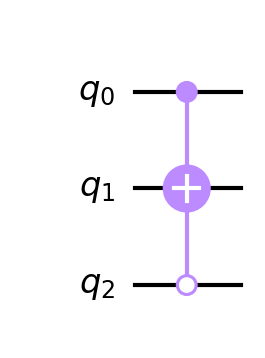
(a) $\tilde{{X}}_{2}=\tilde{X}^{1}_{0}$

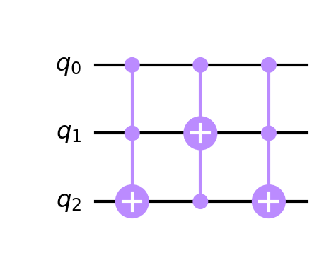
(b) $\tilde{{X}}_{4}=\tilde{X}^{2}_{0}$

Figure 6: The quantum circuits for $\tilde{{X}}_{(\cdot)}$ unitaries corresponding to internal elements of a quadratic interpolation for a 3-qubit system.

(a) ${Z}_{0}$

(b) ${Z}_{(n_{\mathrm{el}}-1)}$

(c) ${I}_{1}^{-1}$

(d) ${I}^{-1}_{2(n_{\mathrm{el}}-1)}$

Figure 7: The quantum circuits for unitaries corresponding to boundary elements of a quadratic interpolation for a 3-qubit system.

As discussed earlier, the actual size of the vector that can be represented in the quantum computer is $N=\tilde{N}+1$. To account for the additional degree of freedom, the size of the global stiffness matrix is adjusted, and the additional unitaries (and the corresponding circuits) are accounted for in the VQLS algorithm. The global stiffness matrix has an additional row and column as shown below:

$$\mathbf{K}=\begin{bmatrix}\mathbf{K}_{\tilde{N}\times\tilde{N}}&\{0\}_{\tilde{N}\crossproduct 1}\\ \{0\}_{1\crossproduct\tilde{N}}&1\end{bmatrix}_{N\crossproduct N}.$$ (28)

The additional row and column can be written as a combination of unitaries, as shown below:

$$\frac{1}{2}\left({I}-{I}^{-1}_{2n_{\mathrm{el}}}\right),$$ (29)

where

$${I}^{-1}_{2n_{\mathrm{el}}}=\begin{bmatrix}1&0&0&0&\cdots&0\\ 0&1&0&0&\cdots&0\\ 0&0&1&0&\cdots&0\\ \vdots&\vdots&\ddots&\ddots&\ddots&\vdots\\ 0&0&&0&1&0\\ 0&0&0&\cdots&0&-1\end{bmatrix}_{N\crossproduct N}.$$ (30)

The $N^{\mathrm{th}}$ entry in the force vector can be arbitrarily chosen, before normalization, but for simplicity, we take it as zero for our simulations.

4.3 Concatenation of global element matrices

In this section, we present a procedure for reducing the number of global element stiffness matrices by defining the concept of unique elements. Two elements that are non-unique have the same element stiffness matrix and do not interact with each other. In the context of the 1-d heat equation, global element matrices for non-unique elements, e.g. non-adjacent elements with identical element lengths and diffusion coefficients, are combined. These elements form a unique element group, and the total number of unique elements are determined accordingly for a given problem and discretization. The global stiffness matrix is then expressed as the sum of global element matrices corresponding only to these unique elements. The concatenated matrices for each unique element are decomposed into unitaries, which are represented by a series of quantum circuits corresponding to the unitary matrices (other than the identity matrix) of the individual elements within each unique element group. This process is illustrated for both linear and quadratic element discretizations in the following sections.

4.3.1 Linear elements

The number of unique elements is denoted as $n^{\mathrm{uq}}_{\mathrm{el}}$. For generality, it is assumed that the boundary elements are treated as unique elements, although, this assumption can easily be relaxed in special cases. By applying the concept of unique elements, the global stiffness matrix can be expressed as follows:

$$\mathbf{K}=\left(\frac{c^{0}}{2h^{0}}+\sum_{e=1}^{n^{\mathrm{uq}}_{\mathrm{el}}-2}\frac{c^{e}}{h^{e}}+\frac{c^{n^{\mathrm{uq}}_{\mathrm{el}}-1}}{2h^{n^{\mathrm{uq}}_{\mathrm{el}}-1}}\right)I-\frac{c^{0}}{2h^{0}}I_{0}^{-1}-\sum_{e=1}^{n^{\mathrm{uq}}_{\mathrm{el}}-2}\frac{c^{e}}{h^{e}}X^{\mathrm{uq}}_{e}-\frac{c^{n^{\mathrm{uq}}_{\mathrm{el}}-1}}{2h^{n^{\mathrm{uq}}_{\mathrm{el}}-1}}I_{n_{\mathrm{el}}-1}^{-1},$$ (31)

where $X^{\mathrm{uq}}_{e}$ denotes the unitary matrix for the $e^{\mathrm{th}}$ unique element. The expression for $X^{\mathrm{uq}}_{e}$ unitary is given as:

$$X^{\mathrm{uq}}_{e}=X_{e_{0}}X_{e_{1}}\cdots X_{e_{m}},$$ (32)

where $e_{(\cdot)}$ denotes the element number of the non-adjacent elements in the original discretization that are being concatenated, and $X_{(\cdot)}$ denotes the corresponding unitary for that element. In the special case, when all elements have identical lengths and diffusion coefficients, the expression for $X^{\mathrm{uq}}_{1}$ and $X^{\mathrm{uq}}_{2}$ are as shown below:

$$X^{\mathrm{uq}}_{1} = X_{1}X_{3}\cdots X_{n_{\mathrm{el}}-2},$$ (33)

$$X^{\mathrm{uq}}_{2} = X_{2}X_{4}\cdots X_{n_{\mathrm{el}}-3}.$$ (34)

If the boundary elements are combined similarly, then the number of unitaries required to represent the global stiffness matrix is $4$. The largest depth of the circuits corresponding to these unitaries is $\mathcal{O}(N)$.

4.3.2 Quadratic elements

The global stiffness matrix for the quadratic elements can be similarly represented with a reduced number of global element matrices using the concept of unique elements. The boundary elements are again treated as unique elements. The representation obtained for the global element stiffness matrix is shown below:

$$\mathbf{K} =\left(\frac{5c^{0}}{2h^{0}}+\sum_{e=1}^{n^{\mathrm{uq}}_{\mathrm{el}}-2}\frac{15c^{e}}{3h^{e}}+\frac{5c^{n^{\mathrm{uq}}_{\mathrm{el}}-1}}{2h^{n^{\mathrm{uq}}_{\mathrm{el}}-1}}\right)\>I+\frac{c^{0}}{h^{0}}\left(\frac{3}{2}\>Z_{0}-\frac{8}{3}\>X_{1}-\frac{4}{3}\>I_{1}^{-1}\right)$$ (35)

$$\quad\quad+\sum_{e=1}^{n^{\mathrm{uq}}_{\mathrm{el}}-2}\left(\frac{c^{e}}{h^{e}}\left(-\frac{8}{3}\>X^{\mathrm{uq}}_{2e}-\frac{8}{3}\>X^{\mathrm{uq}}_{2e+1}+\frac{1}{3}\>\tilde{X}^{\mathrm{uq}}_{2e}\right)\right)$$

$$\quad\quad+\frac{c^{n^{\mathrm{uq}}_{\mathrm{el}}-1}}{h^{{n^{\mathrm{uq}}_{\mathrm{el}}-1}}}\left(\frac{3}{2}\>Z_{n_{\mathrm{el}}-1}-\frac{8}{3}\>X_{2(n_{\mathrm{el}}-1)}-\frac{4}{3}\>I_{2(n_{\mathrm{el}}-1)}^{-1}\right),$$

where $X^{\mathrm{uq}}_{2e}$, $X^{\mathrm{uq}}_{2e+1}$, and $\tilde{X}^{\mathrm{uq}}_{2e}$ are the unitaries for the $e^{\mathrm{th}}$ unique quad element. The expressions for $X^{\mathrm{uq}}_{(\cdot)}$ unitaries for a unique element are:

$$X^{\mathrm{uq}}_{2e} = X_{2e_{0}}X_{2e_{1}}\cdots X_{2e_{m}},$$ (36)

$$X^{\mathrm{uq}}_{2e+1} = X_{2e_{0}+1}X_{2e_{1}+1}\cdots X_{2e_{m}+1},$$ (37)

where $e_{(\cdot)}$ denotes the element number of quad elements (which can be adjacent in this case, because of the structure of these unitaries) and $X_{(\cdot)}$ denotes the corresponding circuit for that element. The $\tilde{X}^{\mathrm{uq}}_{2e}$ expression is shown below:

$$\tilde{X}^{\mathrm{uq}}_{2e}=\tilde{X}_{2e_{0}}\tilde{X}_{2e_{1}}\cdots\tilde{X}_{2e_{m}},$$ (38)

where $e_{(\cdot)}$ denotes the element number of non-adjacent quad elements.

If all the elements have the same lengths and diffusion coefficients, the unitaries corresponding to the internal unique element are obtained as:

$$X^{\mathrm{uq}}_{2} = X_{2}X_{4}\cdots X_{2n_{\mathrm{el}}-2},$$ (39)

$$X^{\mathrm{uq}}_{3} = X_{3}X_{5}\cdots X_{2n_{\mathrm{el}}-1},$$ (40)

$$\tilde{X}^{\mathrm{uq}}_{2} = \tilde{X}_{2}\tilde{X}_{6}\cdots\tilde{X}_{2(n_{\mathrm{el}}-3)},$$ (41)

$$\tilde{X}^{\mathrm{uq}}_{4} = \tilde{X}_{4}\tilde{X}_{8}\cdots\tilde{X}_{2(n_{\mathrm{el}}-2)}.$$ (42)

If the boundary elements are combined similarly, the number of unitaries required to represent the global stiffness matrix is $8$ plus one additional unitary to make the number of unknowns $2^{n}$ for QC representation.

4.4 Treatment for other boundary conditions

The formulation can be extended to account for Neumann boundary conditions in a straightforward manner. The Neumann (natural) boundary condition contributes to the force vector alone. The force vector is assembled classically including the boundary contributions, and represented using the quantum state vector representation. The construction of the stiffness matrix is performed as described above, but by discarding the boundary circuits used to impose homogeneous Dirichlet conditions.

The non-homogeneous Dirichlet boundary conditions are implemented using the penalty method. Consider the strong form governing equation in Eq. (15) with boundary conditions: $u(x_{1})=\overline{u},\>u(x_{2})=0$. For linear elements, the system of equations resulting from the penalty method implementation for the non-zero Dirichlet boundary conditions is shown below:

$$\begin{bmatrix}\frac{c^{0}}{h^{0}}+P&-\frac{c^{0}}{h^{0}}&0&&&\\ -\frac{c^{0}}{h^{0}}&\frac{c^{0}}{h^{0}}+\frac{c^{1}}{h^{1}}&-\frac{c^{1}}{h^{1}}&&&\\ 0&-\frac{c^{1}}{h^{1}}&\ddots&\ddots&&\\ &&\ddots&\ddots&\ddots&\\ &&&\ddots&\ddots&\\ &&&&&-\frac{c^{n_{\mathrm{el}}-2}}{h^{n_{\mathrm{el}}-2}}\\ &&&&-\frac{c^{n_{\mathrm{el}}-2}}{h^{n_{\mathrm{el}}-2}}&\left(\frac{c^{n_{\mathrm{el}}-2}}{h^{n_{\mathrm{el}}-2}}+\frac{c^{n_{\mathrm{el}}-1}}{h^{n_{\mathrm{el}}-1}}\right)\end{bmatrix}\begin{Bmatrix}u_{0}\\ u_{1}\\ \vdots\\ \vdots\\ \vdots\\ u_{N-2}\\ u_{N-1}\end{Bmatrix} =\begin{Bmatrix}f_{0}+P\overline{u}\\ f_{1}\\ \vdots\\ \vdots\\ \vdots\\ f_{N-2}\\ f_{N-1}\end{Bmatrix},$$ (43)

where $P$ denotes the penalty parameter. Naturally, the nodal degree of freedom associated with the non-homogeneous Dirichlet boundary condition is also considered an unknown as implied in Eq. (43). The global stiffness matrix is expressed in terms of unitary matrices as follows:

$$\mathbf{K}=\left(\frac{P}{2}+\sum_{e=0}^{n_{\mathrm{el}}-2}\frac{c^{e}}{h^{e}}+\frac{c^{n_{\mathrm{el}}-1}}{2h^{n_{\mathrm{el}}-1}}\right)I-\frac{P}{2}I_{0}^{-1}-\sum_{e=0}^{n_{\mathrm{el}}-2}\frac{c^{e}}{h^{e}}X_{e+1}-\frac{c^{n_{\mathrm{el}}-1}}{2h^{n_{\mathrm{el}}-1}}I_{n_{\mathrm{el}}}^{-1}.$$ (44)

The force vector is classically calculated with the addition of the contribution from the penalty term.

5 Numerical Verification

The Q-FEM framework was implemented using IBM’s Qiskit software stack. Sequential least squares quadratic programming is used as the classical optimizer in the VQLS algorithm–leveraging the SLSQP solver in the SciPy optimization library. Several other optimization approaches exist, including other gradient-based optimizers as well as global optimizers (e.g. evolutionary algorithms). SLSQP was chosen heuristically due to better observed performance compared to other available techniques in the SciPy optimization library. The cost function Jacobian is computed numerically using finite differences.

Firstly, we consider the role of ansatz selection (from among those available in the literature) on problem convergence. Then, we assess the performance of the algorithm for linear and quadratic element discretizations as a function of increasing problem sizes. All the verification results are obtained using the Aer simulator in the Qiskit library, and without incorporating the noise model in the simulator.

5.1 Ansatz testing

The problem used in the ansatz testing is:

$$\frac{d^{2}u(x)}{dx^{2}}+x=0,\quad\forall x\in[0,1],$$ (45)

subjected to homogeneous Dirichlet boundary conditions. We used 4 qubits in the main registry, which implies a discretization of the problem into 16 interior linear elements and 2 boundary linear elements. For the ansatz testing, we used two metrics to quantify ansatz characteristics: expressibility (Expr) and entanglement capability (ENT) [30, 42]. Expressibility aims to quantify how regularly the problem space is being sampled by the ansatz compared to a distribution of Haar random states. A high expressibility indicates the density of sampling of the problem space is relatively even throughout the sample space, while low expressibility indicates uneven sampling and lost information. Entanglement capability aims to describe the degree of quantum entanglement included in the ansatz.

We computed expressibility [42] for the tested ansatzes by determining the Kullback-Liebler divergence between the probability distribution of fidelities of output states generated by randomly sampling the parameters of the ansatzes and the distribution of Haar random states calculated from an analytic expression [30]:

Expr $$= D_{KL}(\hat{P}(F_{\bm{\theta},\bm{\phi}})||P(F_{\text{Haar}})),$$ (46)

$$P(F_{\text{Haar}}) = (N-1)(1-F_{\text{Haar}})^{N-2},$$ (47)

$$F_{\bm{\theta},\bm{\phi}} = |\langle 0|V^{\dagger}(\bm{\phi})V(\bm{\theta})|0\rangle|^{2},$$ (48)

where fidelity $F_{\bm{\theta},\bm{\phi}}$ is the estimation of overlap between two pure states created by sampling the ansatz with two sets of random parameters $\bm{\theta}$, $\bm{\phi}$ [19]. The fidelity $F_{\text{Haar}}$ is a uniform distribution of fidelities representing a purely random sampling of states. The probability density function $P(F_{\text{Haar}})$ has been derived in Ref. [22], and $N=2^{n}$ is the dimension of the Hilbert space. In expressibility computations below, the inner product of 4,000 pairs of ansatz-generated random states were used.

We estimated the entanglement capability for the tested ansatzes by averaging the Meyer-Wallach entanglement measure $Q$ [8, 30]:

ENT $$= \frac{1}{|S|}\sum_{\bm{\theta}_{i}\epsilon S}Q(V(\bm{\theta_{i}})|0\rangle),$$ (49)

$$Q = 2-\frac{2}{n}\sum_{k=1}^{n}\text{Tr}(\rho_{k})^{2},$$ (50)

where $\rho_{k}$ is the density matrix of the $k^{\mathrm{th}}$ qubit, $n$ is the number of qubits, and $S=\{\bm{\theta}_{i}\}$ is the set of sampled parameter vectors. ENT calculations employed 10,000 samples of circuit parameters.

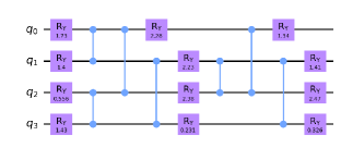
(a) Ansatz 1: this manuscript.

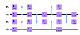
(b) Ansatz 2: Bravo-Prieto et al. [7].

(c) Ansatz 3: Sim et al. [42].

(d) Ansatz 4: Sim et al. [42].

Figure 8: Four ansatzes tested in this study. Only the initial layer and one iterative layer is shown.

The structures of the tested ansatzes are shown in Fig. 8. The ansatzes differ from each other in the entanglement layers. Since Q-FEM searches the solution in real space, we chose ansatzes that exclusively use one-qubit $R_{y}$ rotation gates. To achieve an entangled state, controlled Pauli gates ($CZ$ and $CX$) are employed in different patterns. While Ansatzes 2 [7], 3 and 4 [42] are taken from literature, Ansatz 1 is proposed herein to generalize the ansatz proposed in Ref. [7] to odd number of qubits. We note that this ansatz features two-qubit gates that are not immediate neighbors of each other, which may pose difficulty in qubit arrangement in real quantum computers with imperfect connectivity.

Table 1 provides the overview of the ansatz performance testing and results. Each ansatz was tested in two, three, and four layer configurations. Increasing the number of layers increase the number of ansatz parameters, hence the circuit cost [42]. The ansatzes feature similar numbers of two-qubit gates per layer. For each configuration, Q-FEM was executed 20 times starting from a random initial set of ansatz parameters to assess robustness in achieving converged solution. Success rate (last column in Table 1) refers to the number of simulations that successfully converged. Convergence is assessed when the cost function value at the minima found by the optimization algorithm is less than a tolerance value of $\hat{C}_{p}\leq 10^{-6}$.

A lower Expr value indicates higher level of expressibility, whereas a higher value of ENT (unity as maximum) indicates high entanglement capability. Expressibility and entanglement generally show a consistent and improving trend with increasing layer depths. Success rate also increases with layer depth for all ansatzes tested. Among the four ansatzes tested, Expr and ENT values are most favorable for Ansatzes 1 and 3, respectively. Ansatz 3 demonstrates the highest values of success rate with low number of parameters. Higher layer depth can lead to very flexible circuits capable of producing low entanglement states, which may begin to lower ENT [42], as appears to be the case in Ansatz 3. Expr saturation is also observed in Ansatz 3 behavior in the transition from 3 to 4 layer depth, a trend noted for a similar ansatz in Ref. [42]. When the number of parameters is less than or equal to 16, the success rate is generally low. This trend is attributed to the observation that the size of the system of linear equations is 16, hence a 16-parameter system (unless degenerate) has a solution, and ansatzes with larger than 16 parameters oversample the space and increase the chances of finding the solution. We note that presence of entanglements results in a highly nonlinear cost function. It is therefore possible to achieve optimal solution with less than 16 parameters, but with low success rate. Note that Ansatz 4 achieved a 5% success rate with only 12 parameters. Prior studies demonstrated well-behaved convergent examples in the context of VQLS, where the linear system size is of orders of magnitude larger than the number of ansatz parameters [7]. However, the condition numbers of the Ising-inspired systems tested in the prior studies are near unity, whereas those that correspond to problems investigated in this manuscript are substantially higher as further discussed below.

Ansatz	Ref	Layers	Expr	ENT	Parameters	Success (%)
1	this manuscript	2	.178	.765	12	0
		3	.124	.823	16	25
		4	.112	.847	20	100
2	Bravo-Prieto et al. [7]	2	.201	.502	16	0
		3	.155	.684	22	100
		4	.134	.684	28	100
3	Sim et al. [42]	2	.153	.881	12	0
		3	.121	.900	16	100
		4	.133	.896	20	100
4	Sim et al. [42]	2	.176	.779	12	5
		3	.136	.838	16	30
		4	.134	.856	20	95

Table 1: Results of the ansatz testing.

Figure 9: Evolution of the cost function with iterations using (a) Ansatz 1, (b) Ansatz 2, (c) Ansatz 3, and (d) Ansatz 4. The left figure in each sub-figure shows various runs and the right figure shows the evolution of mean and standard deviation across the ensemble of runs.

5.1.1 Convergence characteristics

Figure 9 shows the evolution of the cost function as a function of optimization iterations for each of the ansatzes tested in this study. The plots show 20 runs of tested Ansatzes 1-4 with a layer depth of 3 for Ansatzes 2, 3 and a layer depth of 4 for Ansatzes 1, 4. A highly oscillatory pattern towards convergence is evident regardless of the initial state and the choice of the ansatz. This pattern was previously observed in other works as well [47]. We attribute this highly oscillatory behavior to the cost function landscape. Figure 10 illustrates the cost function topology, which is obtained by parametric analysis of the cost function near the global minimum. The topology was calculated for a 3-qubit system, by varying two ansatz parameters while keeping all other parameters fixed at the global minima solution. The cost function topology is marked by barren plateaus with multiple local minima solutions located in sharp valleys (deep gorges). During the optimization iterations, low-cost function gradients computed at barren plateaus resulted in large optimization steps and increased cost function values. Fortunately, large step sizes allow for globally probing the cost function landscape and eventually reaching the minimum. In contrast, step size control (e.g., using line search) results in probing the local vicinity of the initial guess and does not necessarily improve the success rate despite achieving more monotonic behavior.

Ansatzes $1$ and $3$ converge successfully in approximately $100$ iterations and exhibit a similar pattern, while Ansatz $2$ converged in about $120$ iterations. Ansatz $4$ required substantially more iterations in certain cases, where the optimization iterations reached plateau regions, before achieving convergence. The statistical behavior (i.e., the evolution of mean and the standard deviation) shown in Fig. 9 demonstrate a relatively monotonic convergence behavior in the aggregate.

(a) ($\theta_{1},\theta_{2}$)

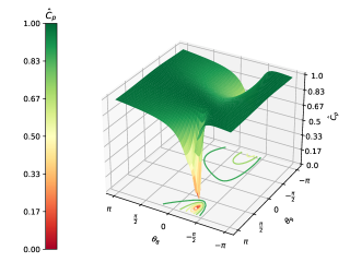
(b) ($\theta_{8},\theta_{9}$)

Figure 10: The field plot for cost function space obtained by varying only two parameters and all other parameters correspond to the minima solution for a 3-qubit linear element discretization example.

5.2 Effect of boundary and force conditions

We proceed with the assessment of the capabilities of Q-FEM by considering linear finite element discretization of the problem in a slightly generalized form $u^{\prime\prime}(x)+b(x)=0$ using a variety of boundary conditions. The grid and the coefficients are taken to be uniform in the examples shown in this section.

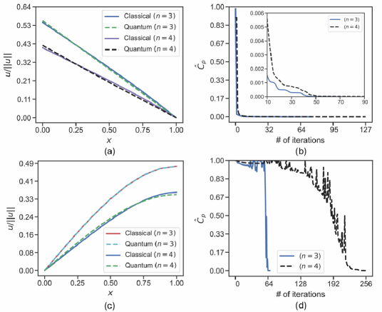
Figure 11: (a) Comparison of Q-FEM and the classical FEM solutions with boundary conditions $u(0)=1$, $u(1)=0$, and $b(x)=x^{2}$. The 3 and 4 qubit solutions are obtained using Ansatz 1. (b) Corresponding evolution of the cost function. Inset figure provides zoom-in view. (c) Comparison of Q-FEM and the classical FEM solutions with boundary conditions $u(0)=0$, $u^{\prime}(1)=0$, and $b(x)=x$. The 3 and 4 qubit solutions are obtained using Ansatz 4. (d) Corresponding evolution of the cost function.

Figure 11a-b shows the results when the boundary conditions are set to $u(0)=1$ and $u(1)=0$, and the forcing function is taken as $b(x)=x^{2}$. The penalty method is used to implement the non-zero Dirichlet boundary condition as discussed in Section 4.4 and for this example the penalty parameter used is $P=100$. The comparison of the normalized solution field obtained by Q-FEM and the classical FEM for $n=3$ and $n=4$ cases are shown in Fig. 11a. Q-FEM results are obtained by setting ansatz layer depth to 2 and 4 for $n=3$ and $n=4$, respectively. We note that the 3-qubit and 4-qubit results do not overlap due to the normalization with respect to the Euclidian norm of the solution vector. Each Q-FEM simulation was repeated 25 times with random initial conditions using Ansatz 1, and 100% of these repeat runs resulted in convergence for 3-qubit, whereas the convergence probability was 92% for the 4-qubit example. Figure 11b shows typical convergence behavior of Q-FEM with Ansatz 1, where the 3-qubit and 4-qubit simulations converged with 75 and 128 iterations, respectively. The convergence behavior of this example is substantially more regular, exhibiting less oscillations and rapid initial convergence compared with Fig. 9, while the average number of iterations to convergence is similar. This observation points to the influence of the boundary condition on the topology of the cost function. We further note that the condition number of the stiffness matrix for the current example (that uses the penalty method to impose non-homogeneous Dirichlet boundary condition) is higher than that for the case with homogeneous Dirichlet boundary conditions reported in Fig. 9.

Figure 11c-d show the results when the boundary conditions are set to $u(0)=0$ and $u^{\prime}(1)=0$. In this example, the forcing function chosen is linear $b(x)=x$. Q-FEM results are obtained by setting ansatz layer depth to 4 for both $n=3$ and $n=4$ cases (layer depth of 2 did not result in high probability of convergence in $n=3$ case). Figure 11d shows typical convergence behavior of Q-FEM with Ansatz 4, where the 3-qubit and 4-qubit simulations converged with 68 and 256 iterations, respectively.

5.3 Problem scaling

The performance of Q-FEM with increasing number of qubits is assessed using the problem defined in Eq. (45). Ansatz 1 was used in the simulations. As the problem size increases, the optimization problem becomes increasingly higher-dimensional as the size of the parameter vector also increases. Numerical testing revealed that the cost function exhibits barren plateaus, leading to the optimization problem either converging to a local minimum or failing to converge within a reasonable number of iterations, even with global optimizers. To solve problems with more than $4$ qubits, we use the classical FEM solution to obtain a good initial guess for the parameters in the ansatz. Previous work, such as [40], has reported the generation of good initial guesses for various problems using quantum computing. This underscores the importance of finding a good initial guess in quantum computing, highlighting the need to design better ansatzes that span the solution space more effectively with as few parameters as possible.

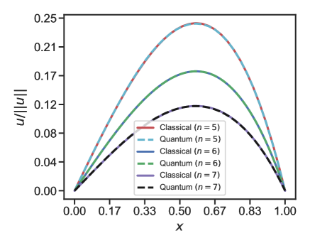
Figure 12: The comparison of Q-FEM solution with the classical FEM solution for homogeneous coefficients and same element lengths for increasing qubits.

# of qubits	Ansatz layer depth	# of parameters
3	2	9
4	4	20
5	6	42
6	13	84
7	22	161

Table 2: Layer depth and parameters in the ansatz to obtain a correct solution with Q-FEM framework for increasing qubits.

Using the generated initial guesses for parameters in the ansatz, we obtain solutions with the Q-FEM framework for increasing problem sizes, which are in good agreement with the classical solution, as shown in Fig. 12. Achieving the correct solution for increasing problem sizes requires the number of parameters in the variational ansatz to scale with the number of unknowns as shown in Table 2. Theoretically, the number of parameters needed to guarantee the existence of the correct solution is equal to the size of the linear system. In practice, using a larger number of parameters increases the probability of convergence and is required as indicated in Table 2.

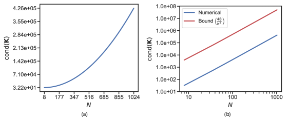
Figure 13: (a) The condition number of the matrix with increasing system size. (b) Comparison of numerically obtained condition number of the matrix and its theoretical bound with system size.

The aforementioned theoretical constraint on the number of parameters is based on a linear representation of the parametric solution space. The variational ansatzes, on the other hand, include nonlinearity primarily due to quantum entanglement. For instance, for the Ising-inspired example problems discussed in Ref. [7], the number of parameters in the ansatz scales linearly with the number of qubits. We speculate that the reason for this scaling is the specific structure of the linear system, which allows the ansatz to span the solution space more effectively with a few parameters. In the current example, the condition number of the global stiffness matrix ($\mathrm{cond}(\mathbf{K})$) increases with the problem size, as shown in Fig. 13a. The numerically obtained $\mathrm{cond}(\mathbf{K})$ for Eq. (45) scales as $\sim N^{2}$, which matches with the theoretical scaling for the upper bound of the condition number, $\mathrm{cond}(\mathbf{K})\leq 48/h^{2}=48(N+1)^{2}$ where $h=1/(N+1)$ is the element length, deduced in [44, Sec. 5.2]. This is evident from the slope of the log-log plot between $\mathrm{cond}(\mathbf{K})$ (numerically obtained and the theoretical bound) and $N$ shown in Fig. 13b. However, this is not observed in the examples considered in [7], where the condition number remains constant regardless of the matrix size. The increasing condition number with system size escalates the time complexity of the optimization problem and raises the potential for encountering barren plateaus and local minima solutions.

5.4 Quadratic elements

In this section, we consider a heterogeneous domain such that $b(x)=x$, $x_{1}=0$, $x_{2}=1$ and $c(x)=1.5$ for $x\in[0,0.41)$ and $c(x)=2.0$ for $x\in(0.41,1]$ in Eq. 15. We discretize the domain into $n_{el}=4$ and $n_{el}=8$ quadratic elements, and the corresponding number of qubits are $n=3$ and $n=4$, respectively. The number of internal nodes for $n=3$ is $N=7$, and for $n=4$ it is $N=15$. As stated previously, we add an auxiliary degree of freedom to represent the stiffness matrix and the force vector in the quantum computer; and without loss of any generality, the corresponding auxiliary entry in the force vector is taken to be $0$. Tables 3 and 4 show the element lengths and coefficients taken for each element in FEM discretization for $n=3$ and $n=4$, respectively.

	$e=1$	$e=2$	$e=3$	$e=4$
$h^{e}$	0.21	0.2	0.235	0.355
$c^{e}$	1.5	1.5	2.0	2.0

Table 3: Element lengths and coefficients for a 3-qubit quadratic element discretization.

	$e=1$	$e=2$	$e=3$	$e=4$	$e=5$	$e=6$	$e=7$	$e=8$
$h^{e}$	0.105	0.105	0.1	0.1	0.125	0.125	0.17	0.17
$c^{e}$	1.5	1.5	1.5	1.5	2.0	2.0	2.0	2.0

Table 4: Element lengths and coefficients for a 4-qubit quadratic element discretization.

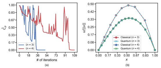
Figure 14: (a) The cost function vs the # of iterations for different qubits with quadratic element discretization. (b) The comparison of Q-FEM solution with the classical FEM solution.

For $n=3$ and $n=4$ examples, the ansatz layer depth is set to 2 and 4, respectively. Figure 14a shows the value of the cost function with the number of iterations for both examples. As evident in Fig. 14a, the sharp changes in the cost function occur during the iterations, as the Q-FEM problem via the VQLS algorithm is a non-convex optimization problem, as discussed previously. Figure 14b shows that the Q-FEM solution matches with the classical FEM solution for both $n=3$ and $n=4$ examples. The 3-qubit and 4-qubit results are different in amplitude because they are normalized with respect to the size of the solution vector.

6 Conclusions

In this work, the Q-FEM framework was developed for use in NISQ computers using the VQLS algorithm. The framework keeps the FEM discretization of the domain intact, which allows the use of variable element lengths and material coefficients, for both linear and quadratic element discretization. The framework is applied to the steady-state heat equation, and a general formalism is developed to generate the quantum circuits corresponding to the unitary decomposition of the stiffness matrix. It is shown through various examples for both linear and quadratic elements discretization that the Q-FEM framework reproduces the classical FEM results, with variable element lengths and non-homogeneous material coefficients.

Several advancements are still needed to leverage the benefits of quantum computing in solving computational mechanics problems. A key difficulty is achieving scalability using the proposed approach. Degradation of the stiffness matrix conditioning with increasing mesh density results in convergence difficulties primarily due to the presence of barren plateaus and the solutions being ‘hidden’ in narrow and deep gorges. New algorithms that can perform efficiently in the presence of badly conditioned problems are therefore necessary. Furthermore, the current manuscript focused on implementation of the generator function approach to compute the unitary matrices for 1-D problems. The generator function approach will need to be generalized to multidimensional discretizations in order to solve more complex problems using the proposed approach. Lastly, future investigations will focus on the verification of the proposed approach in real quantum devices and assessment of Q-FEM’s robustness against errors that exist in the current NISQ devices.

References

- Aaronson [2015] S. Aaronson. Read the fine print. Nature Physics, 11(4):291–293, 2015.
- Ali and Kabel [2023] M. Ali and M. Kabel. Performance study of variational quantum algorithms for solving the poisson equation on a quantum computer. Phys. Rev. Appl., 20:014054, Jul 2023. doi: 10.1103/PhysRevApplied.20.014054. URL https://link.aps.org/doi/10.1103/PhysRevApplied.20.014054.
- Ambainis [2010] A. Ambainis. Variable time amplitude amplification and a faster quantum algorithm for solving systems of linear equations. arXiv preprint arXiv:1010.4458, 2010.
- Araujo et al. [2021] I. F. Araujo, D. K. Park, F. Petruccione, and A. J. da Silva. A divide-and-conquer algorithm for quantum state preparation. Scientific Reports, 11(1):6329, March 2021. ISSN 2045-2322. doi: 10.1038/s41598-021-85474-1. URL https://doi.org/10.1038/s41598-021-85474-1.
- Bausch [2022] J. Bausch. Fast Black-Box Quantum State Preparation. Quantum, 6:773, August 2022. ISSN 2521-327X. doi: 10.22331/q-2022-08-04-773. URL https://doi.org/10.22331/q-2022-08-04-773.
- Bermejo et al. [2024] P. Bermejo, B. Aizpurua, and R. Orús. Improving gradient methods via coordinate transformations: Applications to quantum machine learning. Phys. Rev. Res., 6:023069, Apr 2024. doi: 10.1103/PhysRevResearch.6.023069. URL https://link.aps.org/doi/10.1103/PhysRevResearch.6.023069.
- Bravo-Prieto et al. [2023] C. Bravo-Prieto, R. LaRose, M. Cerezo, Y. Subasi, L. Cincio, and P. J. Coles. Variational quantum linear solver. Quantum, 7:1188, 2023.
- Brennen [2003] G. K. Brennen. An observable measure of entanglement for pure states of multi-qubit systems. Quantum Info. Comput., 3(6):619–626, November 2003. ISSN 1533-7146.
- Cerezo et al. [2021a] M. Cerezo, A. Sone, T. Volkoff, L. Cincio, and P. Coles. Cost function dependent barren plateaus in shallow parametrized quantum circuits. Nat Commun, 12(1791), 2021a. URL https://doi.org/10.1038/s41467-021-21728-w.
- Cerezo et al. [2021b] M. Cerezo, A. Sone, T. Volkoff, L. Cincio, and P. J. Coles. Cost function dependent barren plateaus in shallow parametrized quantum circuits. Nature Communications, 12(1):1791, March 2021b. ISSN 2041-1723. doi: 10.1038/s41467-021-21728-w. URL https://doi.org/10.1038/s41467-021-21728-w.
- Chakraborty et al. [2018] S. Chakraborty, A. Gilyén, and S. Jeffery. The power of block-encoded matrix powers: improved regression techniques via faster hamiltonian simulation. arXiv preprint arXiv:1804.01973, 2018.
- Childs et al. [2017] A. M. Childs, R. Kothari, and R. D. Somma. Quantum algorithm for systems of linear equations with exponentially improved dependence on precision. SIAM Journal on Computing, 46(6):1920–1950, 2017.
- Cleve et al. [1998] R. Cleve, A. Ekert, C. Macchiavello, and M. Mosca. Quantum algorithms revisited. Proceedings of the Royal Society of London. Series A: Mathematical, Physical and Engineering Sciences, 454(1969):339–354, 1998.
- Creevey et al. [2023] F. M. Creevey, C. D. Hill, and L. C. L. Hollenberg. GASP: a genetic algorithm for state preparation on quantum computers. Scientific Reports, 13(1):11956, July 2023. ISSN 2045-2322. doi: 10.1038/s41598-023-37767-w. URL https://doi.org/10.1038/s41598-023-37767-w.
- Feniou et al. [2024] C. Feniou, O. Adjoua, B. Claudon, J. Zylberman, E. Giner, and J.-P. Piquemal. Sparse quantum state preparation for strongly correlated systems. The Journal of Physical Chemistry Letters, 15(11):3197–3205, 2024. doi: 10.1021/acs.jpclett.3c03159. URL https://doi.org/10.1021/acs.jpclett.3c03159. PMID: 38483286.
- Gard et al. [2020] B. T. Gard, L. Zhu, G. S. Barron, N. J. Mayhall, S. E. Economou, and E. Barnes. Efficient symmetry-preserving state preparation circuits for the variational quantum eigensolver algorithm. npj Quantum Information, 6(1):10, January 2020. ISSN 2056-6387. doi: 10.1038/s41534-019-0240-1. URL https://doi.org/10.1038/s41534-019-0240-1.
- Harrow and Napp [2021] A. W. Harrow and J. C. Napp. Low-depth gradient measurements can improve convergence in variational hybrid quantum-classical algorithms. Phys. Rev. Lett., 126:140502, Apr 2021. doi: 10.1103/PhysRevLett.126.140502. URL https://link.aps.org/doi/10.1103/PhysRevLett.126.140502.
- Harrow et al. [2009] A. W. Harrow, A. Hassidim, and S. Lloyd. Quantum algorithm for linear systems of equations. Physical review letters, 103(15):150502, 2009.
- Życzkowski and Sommers [2005] K. Życzkowski and H-J. Sommers. Average fidelity between random quantum states. Phys. Rev. A, 71:032313, Mar 2005. doi: 10.1103/PhysRevA.71.032313. URL https://link.aps.org/doi/10.1103/PhysRevA.71.032313.
- Iten et al. [2016] R. Iten, R. Colbeck, I. Kukuljan, J. Home, and M. Christandl. Quantum circuits for isometries. Phys. Rev. A, 93:032318, Mar 2016. doi: 10.1103/PhysRevA.93.032318. URL https://link.aps.org/doi/10.1103/PhysRevA.93.032318.
- Khatri et al. [2019] S. Khatri, R. LaRose, A. Poremba, L. Cincio, A. T. Sornborger, and P. J. Coles. Quantum-assisted quantum compiling. Quantum, 3:140, 2019.
- Kus et al. [1988] M. Kus, J. Mostowski, and F. Haake. Universality of eigenvector statistics of kicked tops of different symmetries. Journal of Physics A: Mathematical and General, 21(22):L1073, 1988. doi: 10.1088/0305-4470/21/22/006. URL https://dx.doi.org/10.1088/0305-4470/21/22/006.
- LaRose et al. [2019] R. LaRose, A. Tikku, É. O’Neel-Judy, L. Cincio, and P. J. Coles. Variational quantum state diagonalization. npj Quantum Information, 5(1):57, 2019.
- Lee et al. [2021] J. Lee, A. B. Magann, H. A. Rabitz, and C. Arenz. Progress toward favorable landscapes in quantum combinatorial optimization. Phys. Rev. A, 104:032401, Sep 2021. doi: 10.1103/PhysRevA.104.032401. URL https://link.aps.org/doi/10.1103/PhysRevA.104.032401.
- Leone et al. [2024] L. Leone, S. F. E. Oliviero, L. Cincio, and M. Cerezo. On the practical usefulness of the hardware efficient ansatz. Quantum, 8:1395, 2024.
- Levy [1953] S. Levy. Structural analysis and influence coefficients for delta wings. Journal of the Aeronautical Sciences, 20(7):449–454, 1953.
- Liu et al. [2024] Y. Liu, J. Liu, J. R. Raney, and P. Wang. Quantum computing for solid mechanics and structural engineering–a demonstration with variational quantum eigensolver. Extreme Mechanics Letters, 67:102117, 2024.
- Lu et al. [2023] D. Lu, Z. Wang, J. Liu, Y. Li, W.-B. Ewe, and Z. Liu. From ad-hoc to systematic: A strategy for imposing general boundary conditions in discretized pdes in variational quantum algorithm. arXiv preprint arXiv:2310.11764, 2023.
- Meitei et al. [2021] O. R. Meitei, B. T. Gard, G. S. Barron, D. P. Pappas, S. E. Economou, E. Barnes, and N. J. Mayhall. Gate-free state preparation for fast variational quantum eigensolver simulations. npj Quantum Information, 7(1):155, October 2021. ISSN 2056-6387. doi: 10.1038/s41534-021-00493-0. URL https://doi.org/10.1038/s41534-021-00493-0.
- Meyer and Wallach [2002] D. A. Meyer and N. R. Wallach. Global entanglement in multiparticle systems. Journal of Mathematical Physics, 43(9):4273–4278, September 2002. ISSN 0022-2488. doi: 10.1063/1.1497700. URL https://doi.org/10.1063/1.1497700. _eprint: https://pubs.aip.org/aip/jmp/article-pdf/43/9/4273/19183190/4273_1_online.pdf.
- Mottonen et al. [2004] M. Mottonen, J. J. Vartiainen, V. Bergholm, and M. M. Salomaa. Transformation of quantum states using uniformly controlled rotations. arXiv preprint quant-ph/0407010, 2004.
- Nguyen et al. [2024] V.-D. Nguyen, L. Wu, F. Remacle, and L. Noels. A quantum annealing-sequential quadratic programming assisted finite element simulation for non-linear and history-dependent mechanical problems. European Journal of Mechanics - A/Solids, 105:105254, 2024. ISSN 0997-7538. doi: https://doi.org/10.1016/j.euromechsol.2024.105254. URL https://www.sciencedirect.com/science/article/pii/S0997753824000342.
- Perelshtein et al. [2022] M. R. Perelshtein, A. I. Pakhomchik, A. A. Melnikov, A. A. Novikov, A. Glatz, G. S. Paraoanu, V. M. Vinokur, and G. B. Lesovik. Solving large‐scale linear systems of equations by a quantum hybrid algorithm. Annalen der Physik, 534(7), May 2022. ISSN 1521-3889. doi: 10.1002/andp.202200082. URL http://dx.doi.org/10.1002/andp.202200082.
- Pesce and Stevenson [2021] R. M. N. Pesce and P. D. Stevenson. H2zixy: Pauli spin matrix decomposition of real symmetric matrices. arXiv preprint arXiv:2111.00627, 2021.
- Plesch and Brukner [2011] M. Plesch and C. Brukner. Quantum-state preparation with universal gate decompositions. Phys. Rev. A, 83:032302, Mar 2011. doi: 10.1103/PhysRevA.83.032302. URL https://link.aps.org/doi/10.1103/PhysRevA.83.032302.
- Preskill [2018] J. Preskill. Quantum computing in the nisq era and beyond. Quantum, 2:79, 2018.
- Raisuddin and De [2022] O. M. Raisuddin and S. De. Feqa: Finite element computations on quantum annealers. Comput. Methods. Appl. Mech. Engrg., 395:115014, 2022.
- Raisuddin and De [2023] O. M. Raisuddin and S. De. Quantum relaxation for linear systems in finite element analysis, 2023. URL https://arxiv.org/abs/2308.01377.
- Raisuddin and De [2024] O. M. Raisuddin and S. De. Quantum multigrid algorithm for finite element problems. arXiv preprint arXiv:2404.07466, 2024.
- Renaud et al. [2024] N. Renaud, P. Rodríguez-Sánchez, J. Hidding, and P. C. Broekema. Quantum radio astronomy: Quantum linear solvers for redundant baseline calibration. Astronomy and Computing, page 100803, 2024.
- Shende et al. [2006] V. V. Shende, S. S. Bullock, and I. L. Markov. Synthesis of quantum-logic circuits. IEEE Transactions on Computer-Aided Design of Integrated Circuits and Systems, 25(6):1000–1010, 2006. doi: 10.1109/TCAD.2005.855930.
- Sim et al. [2019] S. Sim, P. D. Johnson, and A. Aspuru‐Guzik. Expressibility and entangling capability of parameterized quantum circuits for hybrid quantum‐classical algorithms. Advanced Quantum Technologies, 2(12), October 2019. ISSN 2511-9044. doi: 10.1002/qute.201900070. URL http://dx.doi.org/10.1002/qute.201900070.
- Srivastava and Sundararaghavan [2019] S. Srivastava and V. Sundararaghavan. Box algorithm for the solution of differential equations on a quantum annealer. Physical Review A, 99(5), May 2019. ISSN 2469-9934. doi: 10.1103/physreva.99.052355. URL http://dx.doi.org/10.1103/PhysRevA.99.052355.
- Strang and Fix [2008] G. Strang and G. Fix. An Analysis of the Finite Element Methods, 2nd Edition and Engineering. Wellesley-Cambridge Press, Philadelphia, PA, 2008. doi: 10.1137/1.9780980232707. URL https://epubs.siam.org/doi/abs/10.1137/1.9780980232707.
- Subaşı et al. [2019] Y. Subaşı, R. D. Somma, and D. Orsucci. Quantum algorithms for systems of linear equations inspired by adiabatic quantum computing. Physical review letters, 122(6):060504, 2019.
- Tilly et al. [2022] J. Tilly, H. Chen, S. Cao, D. Picozzi, K. Setia, Y. Li, E. Grant, L. Wossnig, I. Rungger, G. H. Booth, and J. Tennyson. The variational quantum eigensolver: A review of methods and best practices. Physics Reports, 986:1–128, 2022. ISSN 0370-1573. doi: https://doi.org/10.1016/j.physrep.2022.08.003. URL https://www.sciencedirect.com/science/article/pii/S0370157322003118. The Variational Quantum Eigensolver: a review of methods and best practices.
- Trahan et al. [2023] C. J. Trahan, M. Loveland, N. Davis, and E. Ellison. A variational quantum linear solver application to discrete finite-element methods. Entropy, 25(4):580, 2023.
- Wossnig et al. [2018] L. Wossnig, Z. Zhao, and A. Prakash. Quantum linear system algorithm for dense matrices. Physical review letters, 120(5):050502, 2018.
- Zhang et al. [2022] H.-K. Zhang, C. Zhu, G. Liu, and X. Wang. Fundamental limitations on optimization in variational quantum algorithms. arXiv preprint arXiv:2205.05056, 2022.