On Time-Changed Linear Birth-Death Process with Immigration at Extinction
Abstract.
We study an immigration effect in the time-changed linear birth-death process where the immigration occurs only if the population goes extinct. We call this process as the time-fractional linear birth-death process with immigration (TFLBDPwI). Its transient probabilities are obtained using the Adomian decomposition method. In a particular case, we discuss the accuracy of approximation for the obtained transient probabilities. Also, the first two moments of TFLBDPwI are derived. Later, we consider some particular cases of the TFLBDPwI and study their distributional properties in detail.
Key words and phrases:
linear birth-death process, inverse stable subordinator, fractional derivative2010 Mathematics Subject Classification:
Primary : 60J27; Secondary: 60J201. Introduction
Birth-death process is a continuous-time Markov process used to model population growth over time. It has wide applications in both theoretical and practical contexts, such as modeling queues in service systems, epidemics, inventory systems, and the evolution of biological populations. In the linear birth-death process (see [13], p. 456), the state zero is an absorbing state, that is, once the population get extinct it cannot be revived again. Thus, the linear birth-death process is not a suitable model for applications dealing with real-life situations where the population starts from zero. In such cases, a birth-death process with immigration is more appropriate. Recently, Kataria and Vishwakarma [18] studied an immigration effect in the time-changed linear birth-death process where the immigration can happen at any state. For some recent works on the birth-death processes with immigration, we refer the reader to [11], [12] and [17].
Here, we consider the effect of immigration in the linear birth-death process only when the population get extinct. We call this process as the linear birth-death process with immigration (LBDPwI) and denote it by . Let for all be the birth rates and for all be the death rates. Here, and are positive constants and is the rate of immigration. Then, the state probabilities , of LBDPwI solve the following system of differential equations:
| (1.1) |
where for all . If no individual is present at time then the initial conditions are and for all . From (1.1), the probability generating function (pgf) , of LBDPwI solves
| (1.2) |
with
Over the past two decades, many random time-changed and time-fractional growth processes, for example, the fractional Poisson process (see [8], [19], [20]), the fractional pure birth process (see [22]), and the fractional linear birth-death process (see [23]), have been studied. A key feature of these fractional processes is global memory, which characterizes many real-world systems.
In this paper, we introduce and study a time-changed variants of the LBDPwI with an inverse -stable subordinator (for definition see Section 2.1). We call it as the time-fractional linear birth-death process with immigration (TFLBDPwI) and denote it by . It is defined as , where and are independent and . It is shown that the state probabilities of TFLBDPwI satisfy the following system of fractional differential equations:
| (1.3) |
with the initial conditions and for all . Here,
is the Caputo fractional derivative whose Laplace transform is given by (see [15])
| (1.4) |
In the last section, we consider two particular cases of the LBDPwI and study their time-fractional variants. First, we introduce and study the time-fractional linear birth process with immigration and then the time-fractional linear death process with immigration. For both the processes, we obtain the explicit form of their state probabilities, means and variances.
As the TFLBDPwI has immigration effect, it has potential applications to model phenomena with rapidly changing conditions in which the state zero is not observable. For example, it can be used to model the rapid spread of a virus in a particular region. Initially, no individual in the population is infected with the virus however at some point of time someone gets infected due to the migration from outside. Here, we assume that every individuals present within the population are subject to an identical birth and death rates. It is done to prevent variation in the population wellness.
Next, we give a brief introduction of the Adomian decomposition method (ADM).
1.1. Adomian decomposition method
It is a numerical method for solving functional equations. Let us consider the following functional equation:
| (1.5) |
where is a non-linear operator and is a known function. In ADM, it is assumed that the solution of (1.5) and operator can be expressed in terms of absolutely convergent series and , respectively, where is called the th Adomian polynomial in (see [1]-[6], [24]). So, (1.5) can be rewritten as follows:
In ADM, the series components are obtained by using the following recurrence relation:
Note that determining the Adomian polynomials is a key component in this method. Adomian [2] introduced a method to derive these polynomials by introducing a parameterization of the solution . However, if is a linear operator, for example, then ’s are simply . For some recent work related to the Adomian polynomials, we refer the reader to [9], [10] and [16].
2. Time-fractional LBDPwI
Here, we introduce a time-changed version of the LBDPwI where the time is changed according to an inverse stable subordinator. First, we recall the definitions of stable subordinator and its inverse.
2.1. Subordinator and its inverse
A Subordinator is non-decreasing Lévy process (see [7]).
Let , be a subordinator with , . Then, it is called -stable subordinator. The first passage time of -stable subordinator is called an inverse -stable subordinator. Its Laplace transform is given by (see [20])
| (2.1) |
Let be the LBDPwI as defined in Section 1. We consider a time-changed process defined as follows:
| (2.2) |
where the inverse -stable subordinator is independent of the LBDPwI and for all . We call this process as the time-fractional linear birth-death process with immigration (TFLBDPwI).
The following result provides the system of differential equations that governs the state probabilities of TFLBDPwI.
Theorem 2.1.
The state probabilities , of TFLBDPwI solve the system of differential equations given in (1.3).
Proof.
For and , from (2.2), we have
| (2.3) |
Let be the Laplace transform of state probabilities of LBDPwI. Then, on taking the Laplace transform on both sides of (2.3) and using (2.1), we have
| (2.4) |
On taking the Laplace transform on both sides of (1.1), we get
where for all and . So,
| (2.5) |
On substituting (2.4) in (2.5) and using for all , we have
which on taking the inverse Laplace transform and using (1.4) yields
This completes the proof. ∎
Remark 2.1.
Let be a random process whose distribution function is the folded solution of the following fractional diffusion equation:
with and Then, from Theorem 3.1 in [20], it follows that for , where denotes the equality in distribution. Thus, the LBDPwI and TFLBDPwI satisfies the following time-changed relationship:
where is independent of . A similar relationship holds for some other fractional processes, for example, the fractional Poisson process (see [20]), the fractional birth process (see [22]) and the fractional linear birth-death process (see [23]).
2.2. Statistical properties of TFLBDPwI
In this section, we derive the expression for state probabilities of TFLBDPwI and study some of its distributional properties. Note that there are no nonlinear terms involved in the system of differential equations corresponding to the TFLBDPwI. Thus, the ADM can be used to solve (1.3) to obtain the state probabilities of TFLBDPwI. First, we recall the definition of fractional integral and one related result.
Definition 2.1.
Let be an integrable function. Then, the Riemann-Liouville fractional integral is defined as follows (see [15]):
where denotes the fractional integral operator of order .
For , we have the following integral:
| (2.6) |
Note that the Riemann-Liouville integral operator , is linear. So, the Adomian polynomial ’s associated with it are given by .
Now, on applying on both sides of (3.1) and substituting for all , we get
| (2.7) |
By using ADM, we have
| (2.8) |
and for
| (2.9) |
The following result provides the condition under which the series components of the state probabilities of TFLBDPwI vanish. Its proof follows by using the method of induction. A similar result holds in the case of fractional Poisson random fields on positive plane studied in [17]. However, in this case, we deal with only one fractional integral operator, whereas their we have two fractional integral operators of different orders. Also, the system of differential equations appearing here is different from there.
Proposition 2.1.
Let , , be the series components as defined in (2.9). Then, for , we have for all .
Proof.
It is sufficient to show that , for all and . From (2.8), we note that the result holds for and for any .
Now, suppose the result holds for some and for all , that is, . Then, from (2.9), we have
where we have used the induction hypothesis. This completes the proof using method of induction. ∎
Now, we explicitly derive some of the series components. From (2.9), we have . By using (2.6) and (2.8), we get .
Thus, for all and , we can derive the series components of the state probabilities of TFLBDPwI, recursively. However, for arbitrary , and , it is not possible here to determine the closed form of these series components. So, for the computation purpose, we only consider the case where it is possible to do so.
Theorem 2.2.
For and , the series components of the state probabilities of TFLBDPwI are given by
| (2.11) |
where , , and such that whenever for all and .
Proof.
For and such that , the result follows from Proposition 2.1. If then . So, from (2.10), the result holds for .
Let us assume that (2.11) holds for and for some . Then, we have the following three cases:
Case I. For and , from (2.9), we have
where we have used induction hypothesis to get the second equality. Thus, the results holds for and .
Case II. Let . Then, for in (2.9), we have
where again the second equality follows from induction hypothesis. So, the result holds for and .
Case III. If and then the result follows from Proposition 2.1. Now, suppose . Then, and from (2.9), we get
where we have used since .
If then . So,
where we have used to get .
On summing (2.11) over , we get the following result.
Theorem 2.3.
For , state probabilities of the TFLBDPwI are given by
| (2.12) |
where is called the extinction probability.
Remark 2.2.
Note that for , the pgf of TFLBDPwI solves the following fractional differential equation:
| (2.13) |
with initial condition . So, on taking the derivative with respect to on both sides of (2.13) and substituting , we get the governing differential equation for its mean as follows:
| (2.14) |
with . On taking the Laplace transform on both sides of (2.14) and using (1.4), we get
So,
| (2.15) |
whose inversion yields
Now, on taking the derivative twice with respect to on both sides of (2.13) and substituting , we have
with , where is the second factorial moment of TFLBDPwI. By using (1.4) and (2.15), its Laplace transform is given by
whose inversion yields
Thus, in the case of , the variance of TFLBDPwI is
Remark 2.3.
Remark 2.4.
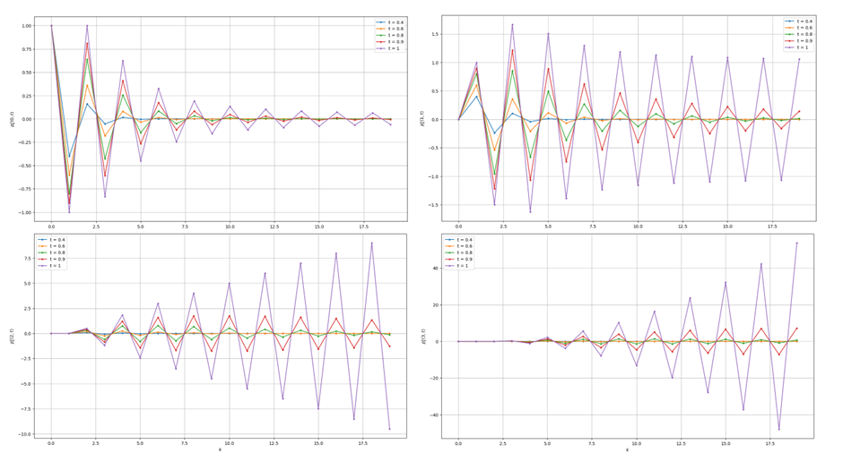
Note that for each the coefficients of the series components is a very rapidly growing sequence of non-negative integers. These coefficients can be calculated by using the given recurrence relation. Moreover, they appear in a triangular array structure which is given as follows:
For , and , the growth of series components for , , , and is illustrated in Figure 1. It can be observed that for , as increases, the series components approach zero, with the convergence rate decreasing as increases. Moreover, for higher values, the deviation from zero becomes larger as increases. Therefore, we conclude that to get a better approximation for the state probabilities for larger values of and , we require a higher number of series components.
3. Some particular cases of TFLBDPwI
In this section, we study the time-changed variants of some particular cases of LBDPwI, such as, the linear birth process with immigration and linear death immigration process.
3.1. Time-fractional linear birth process with immigration
If we allow in LBDPwI then its time-changed version viz TFLBDPwI reduces to a pure linear birth process with positive probability of immigration at state . We call this process as the time-fractional linear birth process with immigration (TFLBPwI) and denote it by , . Its state probabilities solve
| (3.1) |
Similar to the case of TFLBDPwI, we can use the ADM to obtain the state probabilities of TFLBPwI. Let for all . Then, whenever . Moreover, if we allow then the non-zero series components of TFLBDPwI will reduce to for all which are given as follows:
Theorem 3.1.
For , the series components of the state probabilities of TFLBPwI are given by
| (3.2) |
Proof.
The proof follows along the similar lines to that of Theorem 2.2. Hence, it is omitted. ∎
Theorem 3.2.
The state probabilities of TFLBPwI are
| (3.3) |
where is the Mittag-Leffler function defined as (see [15])
| (3.4) |
Proof.
For , on summing (3.2) over the range of , we get
and
where we have used , and
| (3.5) |
for all . This establishes the required result. To show that (3.5) holds true, we proceed as follows:
which on taking derivative with respect to yields
| (3.6) |
On taking the derivative of order on both sides of (3.6) and substituting , we get (3.5). ∎
Alternatively, we can use the Laplace method to obtain the state probabilities (3.3). The following result gives the explicit form of the Laplace transform of the state probabilities of TFLBPwI.
Theorem 3.3.
The Laplace transforms of the state probabilities of TFLBPwI are given by
| (3.7) |
Proof.
On taking in (3.1), we get with initial condition On using (1.4), its Laplace transform is given by . For in (3.1), we get
| (3.8) |
with . On taking Laplace transform on both sides of (3.8) and using (1.4), we get
So, (3.7) holds true for . Let us assume that it holds true for some , where , that is,
| (3.9) |
For , from (3.1), we have
| (3.10) |
On taking the Laplace transform on both sides (3.10) and using (3.9), we get
Thus, the proof is complete by using the method of induction. ∎
Remark 3.1.
On taking the inverse Laplace transform of (3.7) and using the following result (see [15])
| (3.11) |
we get the state probabilities of TFLBPwI as follows:
| (3.12) |
which agree with (3.3).
In particular, for , the TFLBPwI reduces to the linear birth process with immigration. Its probability mass function is
Remark 3.2.
If denotes the waiting time of the TFLBPwI in state then it follows Mittag-Leffler distribution with parameter , that is, , .
Remark 3.3.
If the rate of immigration is sufficiently small enough such that it just trigger the process, that is, for all and , where as , then
So, from (3.12), the state probabilities of TFLBPwI reduces to and
For , we get
Theorem 3.4.
The state probabilities (3.3) satisfy the regularity condition, that is,
Proof.
Remark 3.4.
Theorem 3.5.
The Laplace transform of the pgf of TFLBPwI is given by
3.2. Time-fractional linear death process with immigration
Suppose we allow in LBDPwI then its time-changed version viz TFLBDPwI reduces to the time-fractional linear death process with immigration (TFLDPwI). We denote it by . So, the TFLDPwI can attain only two possible states that are state and state . For any , the marginal distribution of is Bernoulli with success probability . The state probabilities of TFLDPwI solve
| (3.19) |
with . Let . On taking the Caputo fractional derivative on both sides of (3.19) and using , we get with initial condition By using (1.4), the Laplace transform of is Its inverse Laplace transform gives
| (3.20) |
with . On taking the Laplace transform on both sides of (3.20), we get
By taking inverse Laplace transform, we obtain
| (3.21) |
Now, on substituting (3.20) and (3.21) in (3.19), we get
Remark 3.5.
For , the TFLDPwI reduces to a linear death process with immigration. In this case, the state probabilities are given by
References
- [1] Adomian, G., 1984. A new approach to nonlinear partial differential equations. J. Math. Anal. Appl. 102, 420-434.
- [2] Adomian, G., 1985. Non-linear stochastic dynamical systems in physical problems. J. Math. Anal. Appl. 111(1), 105-113.
- [3] Adomian, G., 1986. Nonlinear Stochastic Operator Equations. Academic Press, Orlando.
- [4] Adomian, G., 1986. Systems of nonlinear partial differential equations. J. Math. Anal. Appl. 115, 235-238.
- [5] Adomian, G., Rach, R., 1986. On composite nonlinearities and the decomposition method. J. Math. Anal. Appl. 113, 504-509.
- [6] Adomian, G., 1994. Solving Frontier Problems of Physics: The Decomposition Method. Kluwer Academic, Dordrecht.
- [7] Applebaum, D., 2004. Lévy Processes and Stochastic Calculus. Cambridge University Press, New York.
- [8] Beghin, L., Orsingher, E., 2009. Fractional Poisson processes and related planar random motions. Electon. J. Probab. 14(61), 1790-1826.
- [9] Duan, J.S., 2010. Recurrence triangle for Adomian polynomials. Appl. Math. Comput. 216, 235-1241.
- [10] Duan, J.S., 2011. Convenient analytic recurrence algorithms for the Adomian polynomials. Appl. Math. Comput. 217, 6337-6348.
- [11] Di Crescenzo, A., Martinucci, B., Rhandi, A., 2016. A multispecies birth-death-immigration process and its diffusion approximation. J. Math. Anal. Appl. 442, 291-316.
- [12] Dessalles, R., D’Orsogna, M., Chou, T., 2018. Exact steady-state distributions of multispecies birth-death-immigration processes: effects of mutations and carrying capacity on diversity. J. Stat. Phys. 173, 182-221.
- [13] Feller, W., 1968. An Introduction to Probability Theory and Its Applications, Vol. 1, 3rd ed. Wiley, New York.
- [14] Kirschenhofer, P., 1996. A note on alternating sums. Electron. J. Combin. 3, 1-10.
- [15] Kilbas, A.A., Srivastava, H.M., Trujillo, J.J., 2006. Theory and Applications of Fractional Differential Equations. Elsevier Science B.V., Amsterdam.
- [16] Kataria, K.K., Vellaisamy, P., 2016. Simple parametrization methods for generating Adomian polynomials. Appl. Anal. Discrete Math. 10(1), 168-185.
- [17] Kataria, K.K., Vishwakarma, P., 2024. Fractional Poisson random fields on . arXiv:2407.15619v1
- [18] Kataria, K.K., Vishwakarma, P., 2024. On time-changed linear birth-death-immigration process. J. Theor. Probab. (to appear)
- [19] Laskin, N., 2003. Fractional Poisson process. Commun. Nonlinear Sci. Numer. Simul. 8(3–4), 201–213.
- [20] Meerschaert, M., Nane, E., Vellaisamy, P., 2011. The fractional Poisson process and the inverse stable subordinator. Electron. J. Probab. 16, 1600-1620.
- [21] Orsingher, E., Beghin, L., 2004. Time-fractional telegraph equations and telegraph processes with Brownian time. Probab. Theory Relat. Fields. 128, 141-160.
- [22] Orsingher, E., Polito, F., 2010. Fractional pure birth processes. Bernoulli. 16, 858-881.
- [23] Orsingher, E., Polito, F., 2011. On a fractional linear birth-death process. Bernoulli. 17(1), 114-137.
- [24] Rach, R., 1984. A convenient computational form for the Adomian polynomials. J. Math. Anal. Appl. 102, 415-419.
- [25] Vishwakarma, P., Kataria, K.K., 2024. On the generalized birth-death process and its linear versions. J. Theor. Probab. 37, 3540-3580.