The geometry of the Deep Linear Network
Abstract.
This article provides an expository account of training dynamics in the Deep Linear Network (DLN) from the perspective of the geometric theory of dynamical systems. Rigorous results by several authors are unified into a thermodynamic framework for deep learning.
The analysis begins with a characterization of the invariant manifolds and Riemannian geometry in the DLN. This is followed by exact formulas for a Boltzmann entropy, as well as stochastic gradient descent of free energy using a Riemannian Langevin Equation. Several links between the DLN and other areas of mathematics are discussed, along with some open questions.
1. Introduction
In its simplest form, deep learning is a version of function approximation by neural networks, where the parameters of the network are determined by given data. The best fit is determined, or the network is trained, by minimizing an empirical cost function using gradient descent. Many of the mysteries of deep learning concern training dynamics: Do we have convergence? If so, how fast and to what? How do we make training more efficient? How do the training dynamics depend on the network architecture or on the size of data?
This article focuses on mathematical foundations. Our goal is to illustrate the utility of the geometric theory of dynamical systems for the study of these questions. While gradient flows have been studied in mathematics since the 1930s, gradient flows arising in deep learning have two subtle aspects –overparametrization and degenerate loss functions – that prevent naive applications of the standard theory of gradient flows (see Section 3.2) . We present a geometric framework for a simplified model, the Deep Linear Network (DLN), where these aspects can be studied with complete rigor.
The DLN is deep learning for linear functions. This reduces the training dynamics to gradient flows on spaces of matrices. Despite its apparent simplicity, the model has a rich mathematical structure. Overparametrization provides a foliation of phase space by invariant manifolds. Of these, there is a fundamental class of invariant manifolds, the balanced manifolds, which are themselves foliated by group orbits. This geometric structure allows us to define a natural Boltzmann entropy (the logarithm of the volume of a group orbit) that may be computed explicitly. Microscopic fluctuations that underlie the entropy may be described by Riemannian Langevin equations. This approach unifies the work of several authors into a thermodynamic framework. In particular, it suggests an entropic origin for implicit regularization.
My view is that the DLN is a gift to mathematics from computer science. On one hand, it is subtle, but tractable, providing a rich set of practical questions and insights. On the other hand, the study of the DLN is filled with sharp theorems, exact formulas and unexpected mathematical structure. While the gradient dynamics of the DLN are different from the standard theory, we also see familiar aspects in surprising combinations. This gives the analysis a classical feel, even though all the results here were obtained in the very recent past. There is plenty more to be discovered and the real purpose of this article is to explain why.
In order to apply the methods of dynamical systems theory, what is of most value is to understand the dynamicists ‘way of seeing’. This is not so much a collection of theorems, as a systematic use of geometry, and particular examples, to figure out what questions one should ask. Geometric methods provide a powerful intuition that is often a source of new discoveries.
This is the approach we use in this article. All the theorems we prove are guided by the work of computer scientists in the area. While this article does include some advanced mathematics, especially Riemannian geometry and random matrix theory, we stress explicit calculations, heuristic insights and representative examples. We hope this approach reveals the conceptual power of dynamical systems theory while remaining of interest to practitioners. The references are representative, not exhaustive, since our aim in this article is to provide a pedagogical treatment. We include a brief discussion of the literature on the DLN in Section 13.2. For broader surveys of deep learning that include related mathematical ideas, the reader is referred to the recent books [1, 37].
The article concludes with open questions that emerge from this perspective. These include specific mathematical questions on the DLN, as well as the extension of our entropy formula to gauge groups arising in deep learning.
2. A caricature of deep learning
In its simplest mathematical variant, the purpose of deep learning is to create a function given a collection of training data , with , and denoting the size of the training dat set. In contrast with approximation by a linear combination of basis functions, such as the use of Fourier series or polynomials, in deep learning a function is approximated using neural networks. The neural network consists of individual function elements (neurons) and a hierarchical architecture (the network) so that complicated functions can be constructed by scaling, translating and composing sums of the basic function element. The parameters, denoted for convenience , of the neural network describe the underlying scaling and translation (see [15, p.5] for explicit descriptions).
The parameters are determined from the data by minimizing an empirical loss function. A natural example is the quadratic loss function
| (2.1) |
The parameters are then obtained by minimizing the loss function using gradient descent. We model this process with the differential equation
| (2.2) |
where denotes the gradient with respect to the Euclidean norm in . In practice, the gradient descent is discrete in time, relies on the back-propagation algorithm, and includes random batch processing. These dynamics involve subtle corrections to the gradient flow (2.2), but for the purposes of rigorous analysis, it is is first necessary to have an understanding of equation (2.2).
Our aim in this article will be to foster a geometric understanding of training dynamics for deep networks. In order to do so, we first form a geometric picture of the underlying approximation theory. We will then use the DLN to make precise several aspects of this geometric picture. Here are the important ideas in our work.
-
(1)
Riemannian submersion. The creation of a function by the neural network defines a map . The image of this map, , is the class of functions that can be created with the network. We will visualize this by thinking of the parameter space as living ‘upstairs’ and its image living ‘downstairs’. The natural geometric relation between these spaces is provided by Riemannian submersion.
-
(2)
Scale-by-scale composition. Simple architectural motifs define the architecture for bump functions [28, 33]. Thus, intuitively deep networks form complicated functions through the scale-by-scale composition of bump functions. The expressivity of the deep network – its ability to approximate complicated functions – is quantified by the ‘size’ of . The word size is in quotes, because of the complexity of the map and the fact that is infinite-dimensional. However, this idea may be explored with approximation theory and numerical experiments [15].
-
(3)
The geometry of overparametrization. The problem is overparametrized when the same function may be created with different choices of weights . Precisely, given we must understand a ‘large’ inverse image . It is natural to assume at first that is a manifold. Then defines a set of ‘null directions’ for the gradient descent. (Since the loss function depends on through alone it does not change when is varied along the directions in .) If is large, then the gradient descent is restricted to a ‘thin’ set of directions in . We will quantify these ideas precisely for the DLN with a Boltzmann entropy. Further, we show that noise in the null directions, gives rise to motion by curvature.
-
(4)
Degenerate loss functions. While the loss function is quadratic, there may be many choices of such that the empirical loss function is minimized for such (for example, when is sufficiently small). Naively, this corresponds to overfitting. For example, sufficiently high-degree polynomials will fit the data, but also generate spurious oscillations in between the data points. The functions created by deep learning do not overfit. Heuristically, this seems to be due to the efficient coding of functions made possible by scale-by-scale composition. However, a rigorous analysis must explain this behavior as a consequence of the training dynamics.
We revisit these ideas at the conclusion of this article. This allows us to compare the DLN and deep learning equipped with a precise geometric understanding of training dynamics in the DLN.
3. The deep linear network
3.1. The model
Given a positive integer , we denote by the space of real matrices; the space of symmetric matrices; the space of anti-symmetric matrices; and the space of positive semidefinite (psd) matrices. Finally, denotes the orthogonal group of dimension and denotes the Stiefel manifold of -frames in .
We fix two positive integer and referred to as the width and depth of the network. The state space for the DLN is . Each point is denoted by
| (3.1) |
We equip with the Frobenius norm so that is Euclidean with the norm
| (3.2) |
We define the projection and the end-to-end matrix by111It is not necessary to assume that all the matrices are . All that is required is that the matrix multiplication in equation (3.3) is well-defined. However, we restrict attention to square matrices to illustrate the main ideas.
| (3.3) |
We assume given an energy . The training dynamics are described by the gradient flow in with respect to the Frobenius norm of the ‘lifted’ loss function
| (3.4) |
This is a collection of equations in
| (3.5) |
A computation using equation (3.3) (see Section 7.1.1) simplifies equation (3.5) to
| (3.6) |
Here denotes the matrix with entries
| (3.7) |
This article focuses on the analysis of this gradient flow.
3.2. A comparison with deep learning
Let and let define the linear function for . Then the linear function corresponding to the matrix is . The output function depends only on the end-to-end matrix . However, the same function may be represented by choices of training parameters . Thus, despite the absence of the nonlinear activation element and shifts as in a neural network, the choice of variables in the DLN models overparametrization.
Natural learning tasks for the DLN, such as matrix completion, give rise to degenerate loss functions. Assume given a subset and assume given the values of , for , say . The task in matrix completion task is to obtain a principled answer to the question: how do we reconstruct from the partial observations for ?
The DLN may be used to study this question as follows. We define the quadratic loss function
| (3.8) |
and seek the limit of as when solves the gradient flow (3.6).
This loss function is degenerate because it does not depend on the values when the indices do not lie in . Thus, the loss function is minimized on the affine subspace
The analysis of the gradient flow (3.6) lies beyond the standard theory because of the interplay between overparametrization and the degeneracy of the loss function. Here by standard theory, we mean the analysis of gradient flows using the main results on convergence of the gradient flow such as La Salle’s invariance principle and the closely related Barbashin-Krasovskii criterion [9, 29], the use of the Lojasiewicz convergence criterion [27, 40] for analytic loss functions, and the Morse-Smale decomposition of the gradient flow [35] when the loss function is Morse. These results provide the typical framework for the analysis of gradient flows, but they cannot be naively applied to the DLN. The use of La Salle’s invariance principle is not valid when the loss function does not grow sufficiently fast as (for example, for matrix completion). The Morse-Smale decomposition does not hold since is not a Morse function due to overparametrization.
3.3. Main results
The theorems in this article are a composite of results obtained by several authors. They have been chosen to illustrate three geometric aspects.
-
(1)
Foliation by invariant varieties; the -balanced varieties. The phase space is foliated by invariant varieties described by quadratic matrix equations parametrized by . Theorem 1 explains this structure. It is a geometric consequence of ‘thin gradients’ and holds for all .
-
(2)
Riemannian gradient flows. The dynamics on the invariant varieties may be explicitly described when . The variety is itself foliated by manifolds corresponding to with rank , . We refer to these as balanced manifolds, denoted , or simply , when . Each balanced manifold is invariant and the dynamics on the balanced manifolds is described by a Riemannian gradient flow, with a metric that may be computed exactly using Riemannian submersion. This metric has an obvious infinite-depth limit (though the Riemannian submersion itself does not).
-
(3)
Group orbits, entropy and stochastic dynamics. We define a Boltzmann entropy of the form for group orbits on . This entropy may be computed explicitly (see Theorem 10). The microscopic dynamics associated to the entropy are described using a Riemannian Langevin Equation (RLE) which reveals the role of curvature in the dynamics.
The rigorous results are only part of the story. Each of the main theorems formalizes a different form of geometric intuition and was guided by heuristics, numerical experiments and connections with other areas of mathematics. These connections are truly surprising. For example, the balanced varieties have a subtle relation with the theory of minimal surfaces; a special case of the Riemannian geometry of the DLN is the Bures-Wasserstein geometry on ; and the entropy formula is obtained by analogy with Dyson Brownian motion in random matrix theory.
For these reasons, we first state these results along with some background. This allows the reader to obtain an overview of the geometry of the DLN without much baggage. Most proofs are presented in the sections that follow.
4. -balanced varieties are invariant
4.1. Definitions
Denote the coordinates of by
| (4.1) |
Given , consider the system of quadratic equations
| (4.2) |
The solution set defines an algebraic variety that is termed the -balanced variety. We denote it by
| (4.3) |
Not all values of give rise to non-empty . However, given a point , we may use equation (4.2) to define . Thus, the space is fibered by the varieties .
When , equation (4.2) reduces to the important special case
| (4.4) |
These equations define the balanced variety
| (4.5) |
If , the singular values, and thus rank, of each are the same. In Section 5, we use this observation to construct a parametrization which shows that is foliated by manifolds corresponding to the rank , . We refer to the leaf of with rank as the balanced manifold and denote it by . Our main theorems concern the behavior on .
We lack a complete understanding of the singularities of the variety . However, it is easy to check that is a manifold. For each , equation (4.2) is -valued; thus, there are scalar equations. Since we have parameters, we find that
| (4.6) |
Of these, degrees of freedom correspond to an end-to-end matrix and the remaining degrees of freedom correspond to an group orbit. We parametrize in Section 5 to make this explicit. We focus mainly on for simplicity. When we consider the rank-deficient cases, with , the orbits have to be replaced by orbits.
4.2. Dynamics on invariant manifolds
Each variety is invariant under the dynamics. Let us state this assertion precisely.
Assume that and consider the initial value problem
| (4.7) |
This is a differential equation with a locally Lipschitz vector field. Thus, Picard’s theorem guarantees the existence of a unique solution on a maximal time interval containing . Let be given by the initial condition
| (4.8) |
Theorem 1 (Arora, Cohen, Hazan [3]).
The following hold on the maximal interval of existence of solutions to equation (4.7).
-
(a)
The solution lies on the variety .
-
(b)
The end-to-end matrix satisfies
(4.9) where and we have defined the partial products
(4.10)
The specific nature of is irrelevant to Theorem 1. Instead, it reflects a fundamental geometric restriction forced by overparametrization. The gradient vector fields always lie along a ‘thin’ space of dimension in . We explain this point further in Remark 5 below. Theorem 1 tells us that each variety is invariant under the dynamics, but it does not provide a closed description of the reduced dynamics. However, on the balanced manifold we have
Theorem 2 (Arora, Cohen, Hazan [3]).
Assume . The end-to-end matrix satisfies the differential equation
| (4.11) |
Theorem 1 and Theorem 2 are easy to establish (see Section 7). However, despite their simplicity, both Theorems have a fascinating character. The most important structural feature is that equation (4.11) is a Riemannian gradient flow in disguise. We explain this idea below and then conclude with some remarks on these theorems.
4.3. Riemannian gradient descent
We recommend [30] as an introduction to Riemannian geometry. The reader willing to take some definitions on faith can also understand the main ideas in this work without a detailed understanding of Riemannian geometry.
A metric on assigns a length to each tangent vector . Since the tangent space to at any point is itself isomorphic to , a metric is an assignment of lengths of the form
| (4.12) |
The inner-product may be recovered from the polarization identity
| (4.13) |
We define a metric on as follows. Given the depth for every we define the linear map
| (4.14) |
This linear map allows us to rewrite equation (4.11) as
| (4.15) |
We will show that the operator is always invertible when has full rank. In this setting, the structure of equation (4.15) may be understood better. Define
| (4.16) |
It then follows from the polarization identity and the identity that
| (4.17) |
Given a Riemannian manifold and a differentiable function , the Riemannian gradient of is a vector in obtained from the duality pairing
| (4.18) |
In our setting, where is given by equation (4.16) for . Then the left and right hand sides of this equation are
| (4.19) |
A more careful analysis [5] reveals that the assumption that have full rank is not necessary. Following [5] we foliate by rank, defining
| (4.20) |
The balanced manifolds are naturally related to : lies in if and only if . Further, it is shown in [5, §3] that the metric restricts naturally to for . We then have
Theorem 3 (Bah, Rauhut, Terstiege, Westdickenberg [5]).
Equation (4.11) is equivalent to the Riemannian gradient flow on
| (4.21) |
In particular, when , the end-to-end matrix evolves in according to this Riemannian gradient flow.
When evolves according to (4.21) we have the fundamental estimate
| (4.22) |
It follows that when converges to a critical point of , then converges to a critical point of at exactly the same rate. Overparametrization does not change the speed of convergence.
4.4. Remarks on the invariant manifold theorems
Remark 4.
Equation (4.11) was first obtained by using the gradient flow (3.5) and the identity [3]. The underlying metric was then obtained by noting the properties of the map , including its restriction to rank in [5]. These calculations may be explained geometrically using Riemannian submersion as discussed in Section 6.
Remark 5 (Thin gradients).
The space of gradients of loss functions of the form at a point has at most dimensions. To see this, fix and choose linear energies . There are such energies; thus, their gradients form a basis for the space of gradients of energies at . Equation (3.6) then shows that the space of gradients of at has dimensions. However, the dimension of the space is .
Remark 6 (Group orbits).
Since the gradient flow can explore at most directions we have free parameters. Of these, parameters are fixed by the constants . We use this observation to parametrize by using the polar factorization in Section 5. In particular, for each the inverse image is a orbit .
Remark 7 (Global existence and convergence).
The following method for establishing convergence was introduced in [5].
Picard’s theorem provides local existence on an interval with . In order to obtain global existence for , it is only necessary to show that is bounded in time. If so, we have the uniform bounds
| (4.23) |
Thus, we may inductively control ,, in terms of . Since , the bound on is equivalent to a bound on . It then follows from a continuation argument that and if is uniformly bounded on its interval of existence.
Once we have established that remains in a compact set, we may use standard criterion to establish convergence as . When is analytic, the Lojasiewicz criterion implies convergence to a critical point. For , we may use the La Salle invariance principle to classify the -limit set .
Remark 8 (Relation to the Simons cone).
The variety is a conic section in with a parametrization discussed in Section 5. We may understand the balanced manifold explicitly when and . Let
| (4.24) |
Then equation (4.4) reduces to a system of three quadratic equations
| (4.25) | |||||
| (4.26) | |||||
| (4.27) |
When we add equations (4.25) and (4.27) we obtain the Simons cone
| (4.28) |
The Simons cone is a fundamental counterexample in the calculus of variations and geometric measure theory. The variety defined by (4.28) has zero mean curvature at all points and is a local minimizer of the area functional. However, it is not smooth because of the singularity at . On the other hand, there are no such singularities for minimal surfaces in when . Thus, the Simons cone is the simplest stable minimal surface with a singularity, and it manifests only in with .
We see that the balanced manifold is a five-dimensional variety contained within the Simons cone . We will use a stochastic extension of equation (3.5) to shed some light on this unexpected connection.
Remark 9.
The space of positive definite matrices may be equipped with the Bures-Wasserstein metric (see [10] for an exposition). Gradient flows on can be obtained from the DLN as follows. We set and further restrict to the subspace
| (4.29) |
Then is a psd matrix and the metric given by Riemannian submersion of is the Bures-Wasserstein metric .
5. Parametrization of and
5.1. Polar factorization and the SVD
Recall that a matrix admits left and right polar decompositions
| (5.1) |
where and . Further, and are the unique psd square roots of these matrices.
The polar factorization is related to the singular value decomposition (SVD) of as follows. Let us denote the SVD by
| (5.2) |
where and with each . Then we have immediately
| (5.3) |
Therefore, and provide an orthonormal basis of eigenvectors for and respectively. Finally, we have the relation between the factors
| (5.4) |
5.2. Parametrization by the polar factorization
We now parametrize each -balanced variety using the polar factorization, defining a map
| (5.5) |
An interesting feature of equation (4.2) is the manner in which the left and right polar factors alternate along the network as the index varies. We use the polar factors of to rewrite equation (4.2) in the form
| (5.6) |
We define the map as follows. Compute
| (5.7) |
Now proceed algorithmically: as increases, we find sequentially
| (5.8) |
These equations may also be combined into an iterative sequence for . We have
| (5.9) |
Each square-root is a smooth map when is a negative definite matrix. Thus, the variety is a manifold with dimension when each is negative definite.
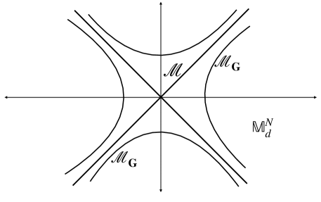
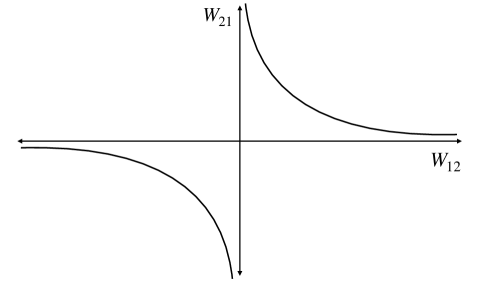
The balanced varieties are matrix-valued conic sections. A useful geometric caricature is obtained by considering the case . 222We switch notation to lower case letters to prevent any confusion with the case . Assume given where each . Then given , we see that is a conic section in described by the hyperbolas
| (5.10) |
Finally, note that the parametrization goes from right to left. We have an analogous parametrization from left to right
| (5.11) |
given for by the sequential polar factorizations
| (5.12) |
5.3. Parametrization by the SVD
The parametrization may be simplified further on the balanced variety . We now have
| (5.13) |
Let us first study the case when has full rank. Then is positive definite and the parametrization continues to be smooth because equation (5.8) reduces to the chain of equalities
| (5.14) |
It follows that each is positive definite and that is locally a manifold. We denote this branch of as and call it the balanced manifold.
The singular values of each are identical on . This allows us to simplify the parametrization further. We define the coordinate map
| (5.15) |
where for each we set
| (5.16) |
Here denotes the singular values of each and denotes the singular values of . Indeed, it follows from equation (5.16) that
| (5.17) |
This parametrization is a local bijection when the singular values are distinct. However, it can fail to be smooth when has repeated singular values. We will compute the metric on in Section 8.
5.4. The rank-deficient case
When has rank , we may extend each of the above parametrizations in a natural way. First, we fix the action of the permutation group on by ordering the singular values
| (5.18) |
Thus, when has rank ,
| (5.19) |
Taking a limit of full-rank matrices in equation (5.16), we see that it is only the first orthonormal vectors in each that affect in the rank-deficient limit. Thus, in order to extend to we must replace the action of in the parametrization with the action of . Then (5.15) extends to the family of parametrizations indexed by ,
| (5.20) |
Equations (5.16)–(5.17) continue to hold true and we see immediately that is also a manifold. The image , where was defined in equation (4.20).
6. Entropy of group orbits and Riemannian submersion
6.1. Overview
In this section, we use Riemannian submersion to develop a thermodynamic framework for the DLN. We restrict ourselves to full rank matrices. The generalization to rank is natural, but it requires that be replaced by and a careful treatment of zero singular values.
6.2. The entropy formula
The parametrization (5.15)–(5.17) allows us to foliate with group orbits as follows. For each consider its preimage in
| (6.1) |
We use equations (5.15)–(5.17) to find that is an orbit of . Indeed, the SVD of fixes , and , leaving free.
We interpret this geometric picture in the language of thermodynamics. Matrices downstairs are macrostates, or observables, whereas matrices upstairs are microstates. Conceptually, the entropy enumerates the number of microstates corresponding to a given macrostate, with the enumeration given by Boltzmann’s formula, , where denote the number of microstates. In our setting, since inherits a metric from its embedding in , the number of microstates associated to is the volume of the group orbit with respect to this metric. This reduces the computation of the entropy to an evaluation of a matrix integral and we find
Theorem 10 (Menon, Yu [34]).
For each with SVD given by (5.17)
| (6.2) |
where is the volume of the orthogonal group with the standard Haar measure.
Here denoted the Vandermonde determinant associated to the matrix as follows:
| (6.3) |
Similar factors appear in a different way in the following
Theorem 11 (Cohen, Menon, Veraszto [14]).
The volume form on is
| (6.4) |
Both theorems follow from explicit computations of metrics, but the two theorems correspond to different metrics. Theorem 11 concerns the metric downstairs and follows easily from Lemma 1. On the other hand, Theorem 10 concerns the metric upstairs as explained in Section 8. It follows from a computation of the pullback metric on the parameter space .
6.3. Equilibrium thermodynamics
Definition 12.
Given we define the Boltzmann entropy
| (6.5) |
At the inverse temperature we define the free energy
| (6.6) |
The introduction of the entropy allows us to extend gradient descent of the energy to gradient descent of the free energy on
| (6.7) |
The geometry of group orbits also allows us to introduce natural microscopic dynamics that capture the notion of ‘fluctuations in the gauge’. In Section 10 we extend equation (6.7) to Riemannian Langevin Equations of the form
| (6.8) |
where is Brownian motion at inverse temperature on .
The inclusion of the entropy provides a selection principle when is degenerate. We expect that a typical solution to equation (6.7) is attracted to the minimizing set
| (6.9) |
At present, we do not understand the structure of this set completely even for the simple energy corresponding to matrix completion (see Section 14). In particular, it is natural to conjecture that consists of a single point and that is selected by the training dynamics due to noise introduced through round-off errors. However, we do not have rigorous results in this direction.
6.4. Riemannian submersion
The metric was first introduced in [5, §3] using an analysis of . The parametrization (5.15)-(5.16) provides a simple geometric explanation for the origin of this metric.
Theorem 13 (Menon, Yu [34]).
For each rank , , the metric on is obtained from the map by Riemannian submersion.
The main ideas in the proof of this theorem are as follows:
- (1)
- (2)
-
(3)
The differential , its kernel and orthogonal complement may be computed explicitly using Theorem 14. We then find an orthonormal basis of and show that the projection of this basis to provides an orthonormal basis for .
7. Proof of Theorem 1–Theorem 3
In this section, we provide the essential steps in the proofs of Theorem 1–Theorem 3. The proofs involve direct matrix calculations. We typically assume the Einstein convention and sum over repeated indices.
7.1. Balanced varieties
7.1.1. Overparametrization and equation (3.6)
Fix , . We must compute the matrix with . By the chain rule, this is the matrix with entries
| (7.1) |
Clearly, the form of is not that important, what really matters is the application of the chain rule to the product . Let us write this as
| (7.2) |
Therefore,
| (7.3) |
which may be rewritten as
| (7.4) |
It then follows from equation (7.1) and (7.4) that
| (7.5) |
7.1.2. Proof of Theorem 1
By the product rule we have
| (7.6) |
We now find from equation (7.5) that
| (7.7) |
where we have observed that
In a similar manner, using equation (7.5) with replaced by we also have
| (7.8) |
Part (a) of Theorem 1 now follows immediately from the identity.
| (7.9) |
Part (b) of Theorem 1 is similar. The factors and defined in equation (4.10) appear naturally in the calculation. We use the chain rule to see that
| (7.10) |
We then apply equation (7.5) to each term, observing that in each case the product above has factors that complement the products and . For example, the first term simplifies to
The general term is given by
We sum over the depth index from to to obtain equation (4.9).
7.1.3. Proof of Theorem 2
Theorem 2 is a specialization of Theorem 1(b) to the balanced variety. Since
on the balanced variety we may simplify the prefactors and appearing in equation (4.9). It follows immediately from equation (4.9) and the parametrization (5.16) that
| (7.11) |
We then have
We substitute in equation (4.9) to complete the proof.
7.2. The Riemannian manifold and Theorem 3
We hold and fixed in this subsection. To simplify notation, we refer to as .
The main observation in this section is that is diagonalized in singular value coordinates. Precisely, let and be the column vectors of and respectively. Then we may write the SVD (5.17) as
| (7.12) |
Lemma 1.
The operator is symmetric and positive definite with respect to the Frobenius inner-product. It has the spectral decomposition
| (7.13) |
when and
| (7.14) |
Proof.
Observe that distinct eigenvectors are orthogonal with respect to the Frobenius metric. Indeed, for each pair of indices and
which vanishes unless the pairs agree. It then follows from the eigendecomposition that is a symmetric and positive definite operator from . ∎
8. Embedding and the metric on
The balanced manifold is a Riemannian manifold since it is locally embedded in and inherits the Frobenius metric, denoted , from . In order to use our parametrization to understand the Riemannian manifold , we must pull back the metric onto the parameter space . In this section, we compute an orthonormal basis for by computing an orthonormal basis for the pullback metric . This is the technical core of [34].
8.1. The tangent space .
First, at each point , we compute the tangent space by differentiating the parametrization (5.16) as follows. The tangent space at the identity to the orthogonal group is the space of antisymmetric matrices, denoted . Thus, if the singular values of are distinct, the parametrization is smooth and for each we may define a smooth curve in using
where is the diagonal matrix and .
Then we obtain a tangent vector in by differentiating in 333Note that the term ‘vector’ here is used to mean ‘vector in the sense of vector space’. Each vector in ‘sits in’ .
| (8.1) |
Explicitly, the -th matrix in is
| (8.2) |
8.2. Computing in the standard basis.
Since the metric on is inherited from its embedding in , the length of each vector
| (8.3) |
is given by the Frobenius norm
| (8.4) |
Similarly, the inner product between two vectors , is given by
| (8.5) |
By linearity, we may reduce the computation of the pullback metric to inner products between the action of on the basis vectors on . We arrange these basis vectors as follows. First, let be the standard basis on and define the image of diagonal matrices
| (8.6) |
Next, form the standard basis for
| (8.7) |
and for each use it to define a tangent vector in by setting
| (8.8) |
Here and we have used the superscript to index depth .
We may now express the pullback metric in the standard basis on by computing the Frobenius inner product between the tangent vectors and the tangent vectors . Let denote the identity matrix. We then have
Lemma 2.
The standard basis on may be ordered such that the pullback metric has the block diagonal structure
| (8.9) |
where is the symmetric tridiagonal matrix
| (8.10) |
There are blocks, each indexed by a basis matrix . This ordering is less intuitive than arranging the metric by depth into blocks, each of size . However, this structure appears naturally in the computation of inner products. It reflects a subtle non-local coupling along the depth of the network that is due to balancedness.
Sketch of the proof.
First, rewrite equation (8.2) as follows
| (8.11) |
Now observe that the linear transformation of the -th tangent space defined by is an isometry for the Frobenius norm. We see immediately that when the image
| (8.12) |
is a collection of diagonal matrices. On the other hand, when ,
| (8.13) |
always vanishes on the diagonal. Thus, the inner-products
| (8.14) |
This gives rise to the block in the upper left corner.
The only non-zero inner products concern , where
| (8.15) |
have overlapping indices and . In this case, we find that the only non-zero inner product corresponds to . The main step involves the identity
| (8.16) |
∎
8.3. An orthonormal basis for .
We may compute an orthonormal basis for by diagonalizing the block tridiagonal matrix of Lemma 2. The diagonalization procedure uses the theory of Jacobi matrices, in particular the fact that the eigenbasis of each block may be computed using Chebyshev polynomials.
The results of this approach may be summarized as follows. Assume that and let us denote the columns of each by
| (8.17) |
We will define a collection of vectors denoted by
| (8.18) | |||||
| (8.19) |
There are vectors of type and vectors of type . The coordinates of these vectors are as follows. First, for the vectors
| (8.20) |
We next consider the vectors for . This range for corresponds to the overparametrization freedom . We define
| (8.21) |
Here we have denoted for brevity
| (8.22) |
Finally, we consider the action of the matrices and that generate the SVD of . First, for define
| (8.23) |
Similarly, define for
| (8.24) |
We then have
Theorem 14 (Menon,Yu [34]).
Theorem 14 is the main tool in the proofs of Theorem 10 and Theorem 13. Let us first explain how Theorem 13 is obtained from it.
In order to show that the metric on is obtained by Riemannian submersion of under we must compute and find an isometry between and . The kernel corresponds to the group action of and it is the span for . Thus, is spanned by the vectors , , and . We see immediately that these correspond exactly to the eigendecomposition of computed in Lemma 1. This establishes that is obtained by Riemannian submersion from .
Theorem 10 is obtained as follows. We must compute the volume of the orbit . We work in local coordinates given by our parametrization, and observe that fixing corresponds to fixing , and . The pullback metric is invariant under the action. This reduces the computation of the group volume to the computation of the determinant of restricted to the subspace spanned by , . This determinant may be computed explicitly using Theorem 14, yielding Theorem 10.
The proof for the rank-deficient case requires more care, but the above arguments captures the essence of these theorems. Further details may be found in [34].
9. Cartoons
The way dynamicists actually work is by drawing pictures that capture different forms of geometric intuition. The purpose of this section is to illustrate this way of thinking, complementing several theorems with an impressionistic visualization of the theorems. A good picture can tell us what a theorem means; or better yet, help us guess what theorems we should be proving.
The DLN is an attractive model because it provides us with a rich set of pictures that suggest new questions for study. We organize our cartoons visually to bring out these aspects, focusing on the following themes:
-
(1)
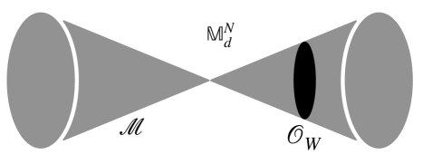
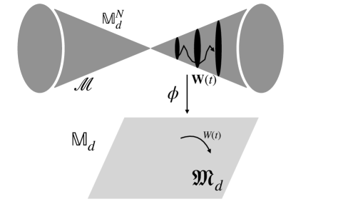
Riemannian submersion. We often organize images into a -space upstairs and -space downstairs. Riemannian submersion arises in several areas of analysis, especially mass transportation, and it is helpful to study the effects of overparametrization in analogy with these areas.
-
(2)
Conic sections. The equations (4.2) that define the balanced varieties are quadratic equations. Thus, when drawing a two or three dimensional sketch, we caricature the balanced varieties by conic sections. This caricature then immediately focuses our attention on the balanced variety .
-
(3)
Foliation by rank. The balanced variety is itself foliated by rank. We have only studied the case in depth, but the rank-deficient case is of great interest. This is harder to visualize, so we have demonstrated the effect of rank within the zero energy set for an example discussed in equations (14.1)–(14.4).
-
(4)
Foliation by group action. The parametrizations by the polar factorization and SVD provide a different way of exploring balanced manifolds with group action. The computation of the pullback metric illustrates the subtle nature of the coupling by depth along the network. We visualize this by slicing the balanced manifold.
-
(5)
Mean curvature is an Itô correction. We often use the fact that the mean curvature from of an embedded manifold is the ‘deterministic push’ that arises from isotropic tangential stochastic fluctuations. This cartoon allows us to introduce Riemannian Langevin equations for the DLN in an intuitive manner. This can be illustrated rather simply and then generalized to more sophisticated foliations, such as in Section 11.1.
10. The Riemannian Langevin equation (RLE)
10.1. Overview
The next three sections address the following question: can we use the DLN to develop the thermodynamics of deep learning?
In the spirit of this article, such a framework must be rooted in the geometry of overparametrization. We have seen that the analysis of the DLN leads naturally to the Riemannian manifolds and . Further, we have used this geometry to define a Boltzmann entropy as well as the gradient descent of free energy (see Section 6). In the physical analogy with thermodynamics, what we are now seeking is an explicit understanding of microscopic fluctuations and Gibbs measures. Our task, therefore, is to develop the underlying ‘statistical physics’ that corresponds to the entropy formula, based on strictly geometric foundations.
In this section, we introduce the Riemannian Langevin Equation (RLE) as the natural geometric model for fluctuations. Our argument is by mathematical analogy and it takes the following form. First, we review the Langevin equation on . We then explain how the RLE is its natural extension to Riemannian manifolds. This is followed by the description of an important example from random matrix theory (Dyson Brownian motion). We then abstract the underlying structure combining Riemannian submersion with the theory of Brownian motion on manifolds. Finally, in Section 12.2, we describe the explicit nature of the RLE in the DLN.
The correspondence between the RLE for the DLN and Dyson Brownian motion is a powerful tool. It provides a way to use ideas from random matrix theory to analyze training dynamics of the DLN. It immediately leads to open questions of intrinsic mathematical interest which are discussed in Section 14. Algorithmically, the RLE replaces the problem of minimizing the free energy with Gibbs sampling.
The RLE is a generalization of the Langevin equation based on the intrinsic Riemannian geometry. We introduce it here as a phenomenological model that incorporates the effect of noise, revealing the interplay of noise and curvature. Whether a mathematical theory works in pratice is a different matter altogether. Our RLE loosely corresponds to how noise due to round-off errors may interact with the geometry of overparametrization. It does not account for the many different ways in which noise actually arises in training dynamics (discretization, batch processing, random initialization,…). Nevertheless, we hope the structure of the RLE will provide a useful framework for practitioners, since it is a reference model which is a natural stochastic analogue of gradient descent (though it is not stochastic gradient descent (SGD) corresponding to batch processing).
10.2. The Langevin equation
First, let us recall the Langevin equation on . Assume given and a potential . The Gibbs measure with respect to this potential is the probability measure with density
| (10.1) |
The Langevin equation describes microscopic stochastic fluctuations in and out of equilibrium. It is the Itô SDE 444We suppress the usual subscript (such as ) in the notation to simplify the SDE for coordinates and matrices.
| (10.2) |
where denotes the standard Wiener process in .
Assume the law of has a density and assume that the law of is given. The evolution of the probability density is then given by the Fokker-Planck (or forward Kolmogorov) equation
| (10.3) |
Under suitable assumptions on , is the Gibbs density defined in equation (10.1).
10.3. RLE: general principles.
The Langevin equation and the Fokker-Planck equation have been widely studied in mathematical physics. Our interest here lies in the generalization of these equation to Riemannian manifolds. The main issue is to understand how to replace the noise in equation (10.2).
Assume given a Riemannian manifold . We define the Laplace-Beltrami operator by its action on a smooth function in coordinates by
| (10.4) |
where denotes the determinant of and denotes its inverse. Brownian motion on at inverse temperature is a diffusion on whose generator is . While the parameter can be included within the metric, we will include it separately, since there are many situations where it is necessary to hold fixed and rescale the strength of the noise.
The abstract characterization of Brownian motion as a diffusion process with a generator is powerful. However, in practice (for example, for simulation) we seek ‘hands-on’ constructions of Brownian motion as the limit of suitable random walks. There are several such constructions of Brownian motion using Stratonovich SDE (see for example [21, §3.2], [23, §V.4], [24, Thm 3]). Once Brownian motion on has been constructed with SDE, it is easy to (formally) extend the Langevin equation (10.2) to the Riemannian setting.
Let denote Brownian motion on at inverse temperature and consider the (formal) Itô SDE
| (10.5) |
This equation is only formal, because SDE on manifolds must be defined using the Stratonovich formulation to ensure coordinate independence. However, equation (10.5) makes the analogy with (10.2) transparent and one may recover the ‘true’ Stratonovich SDE by the inclusion of a drift term computed using the Itô-Stratonovich correction formula. The important geometric aspect for matrix manifolds is that this yields a curvature correction that is often explicitly computable.
11. Curvature and entropy: examples
11.1. Dyson Brownian motion via Riemannian submersion
Dyson Brownian motion at inverse temperature is the interacting particle system described by the Itô SDE
| (11.1) |
Here denotes the standard Wiener process in . This equation has a unique strong solution when that remains confined to the Weyl chamber
| (11.2) |
In [22] we presented a geometric construction of Dyson Brownian motion using Riemannian submersion. This construction has a natural extension to the DLN, but we must first introduce some notation to explain these ideas.
Let denote the space of Hermitian matrices equipped with the norm and let denote the unitary group. Given , let , and let denote the isospectral orbit
| (11.3) |
We observe that the space is foliated by orbits, each of which is an isospectral set, and an isospectral manifold when the elements of are distinct. The main insight in [22] is the interplay between mean curvature, tangential noise, and the entropy that is captured in the following ‘lift upstairs’ of equation (11.1).
Let and let and denote the orthonormal projections onto and respectively with inner-products computed according to . Let denote the standard Wiener process on . For every we define the Itô SDE
| (11.4) |
Assume that is the unique strong solution to equation (11.1) for its maximal interval of existence (this is when ). We then have the following
Theorem 15 (Huang, Inauen, Menon [22]).
-
(a)
The eigenvalues of have the same law as the solution to (11.1) for .
-
(b)
When , the group orbits evolve by motion by (minus one half) mean curvature.
The main insight in the theorem is captured in the case . In this setting, the stochastic fluctuation is tangential to the orbit . However, the Itô correction is minus a half times the mean curvature. In particular, it is deterministic and normal to .
Remark 16.
The entropy formula in Theorem 10 is inspired by the analogous formula for :
| (11.5) |
where is a universal constant. We then see that we may rewrite equation (11.1) as follows 555In [22], we work with Hermitian matrices, which is the most natural setting for Dyson Brownian motions. The factors of that cancel are included for consistency with the general theory of RLE.
| (11.6) |
Remark 17.
The role of in equation (11.1) reflects the standard terminology of random matrix theory. In equation (11.4), however, the parameter reflects an anisotropic splitting of the inner-product in between the tangent space and . For these reasons, we will introduce a separate parameter to describe the anisotropy, and use for the ‘true’ inverse temperature when augmenting equation (11.4) with a loss function.
In order to define stochastic gradient descent by the RLE, we include a loss function in equation (11.4) as follows. Given , set and consider
| (11.7) |
The corresponding equation downstairs is
| (11.8) |
where is the standard Wiener process in and
| (11.9) |
is the free energy. When , we have gradient descent of free energy. In equations (11.7) and (11.8) the gradient operator is with respect to the standard inner products on and respectively. In fact, these metrics are related by Riemannian submersion.
In what follows, we will use equation (11.7) as a model for stochastic gradient descent by the RLE of a loss function, which accounts separately for anisotropic fluctuations in the gauge group and the observable.
11.2. The stochastic origin of motion by mean curvature.
The appearance of mean curvature in Theorem 15(b) may be understood through a simpler example. Let , let denote the length of , and let denote the sphere of radius in . Let denote the orthonormal projection onto ; explicitly, we have
Let denote the standard Wiener process in and consider the Itô SDE
| (11.10) |
This SDE is the continuum limit of a random walk which may be intuitively described as ‘at each time step, take an isotropically distributed random spatial step in the tangent space’.
Stochastic calculus makes it easy to capture the intuitive content of such clumsy verbal descriptions. In particular, since the SDE is in the Itô form, it gives rise to a correction in . The reader is invited to apply Itô’s formula to see that while always evolves by tangential stochastic fluctuations governed by equation (11.10), the radius satisfies
| (11.11) |
The standard normalization of the mean curvature of the sphere is such that it has magnitude and points inwards. Consequently, equation (11.11) tells us that the concentric spheres evolve by motion by minus a half times mean curvature.
12. RLE for stochastic gradient descent
12.1. Riemannian submersion with a group action
In this section, we introduce Riemannian Langevin equations to model stochastic gradient descent of free energy. We formalize the insights obtained in the examples of Sections 11.1– 11.2 in a general geometric framework. We also include ‘lifted’ loss functions as in deep learning. These RLE provide stochastic extensions of gradient flows such as (3.4), which are consistent with the underlying geometry. The tunable parameter modulates the relative strength of the noise in null directions, or equivalently the gauge group, with the noise in the observable. When , we recover Riemannian gradient descent of free energy for the observable.
The geometric assumptions are as follows. We assume given a reference Riemannian manifold and a Lie group of isometries. We then consider the quotient space equipped with the metric given via Riemannian submersion. Let denote the submersion map and let denote the inverse image for each . Then the following general principles hold:
-
(1)
There is always a natural Boltzmann entropy .
-
(2)
The gradient in of the entropy is the mean curvature at each point .
-
(3)
Brownian motion on projects to Brownian motion on . Precisely, if is a diffusion in with generator then is a diffusion on with generator .
The tangent space at each point splits into and its orthogonal complement . Let and be the orthonormal projections onto these subspaces of . The formal analog of the anisotropic splitting in equation (11.7) is
| (12.1) |
The use of stochastic calculus makes it easy to describe the intuitive basis of the anisotropic decomposition and we will use this expression below for its simplicity and suggestive power. Such Itô calculus expressions may be made rigorous in two ways. First, we may use the equivalent Stratonovich SDE, computing the required Itô-Stratonovich correction. Second, it is also possible to avoid stochastic calculus by replacing the standard Laplacian with an anisotropic Laplacian as follows.
Rigorously, the decomposition (12.1) can be expressed using the generator of the process . The orthogonal decomposition allows us to split the Laplacian into ‘angular’ and ‘radial’ Laplacians, denoted by and respectively. Then the anisotropic process is the diffusion with generator
| (12.2) |
An explicit description of an orthonormal basis for is very useful when we apply this idea in practice. In particular, the basis in Section 8.3 is used when we apply these ideas to the DLN.
The energetics are as follows. We assume given a loss function downstairs that we lift to a loss function , .
We then define stochastic gradient descent by the RLE of the loss function through the (formal) Itô SDE ‘upstairs’
| (12.3) |
This equation is an analogue of (11.7). We then expect in analogy with equation (11.8) that the corresponding SDE ‘downstairs’ is
| (12.4) |
with free energy
| (12.5) |
In the limit , we have the stochastic flow upstairs
| (12.6) |
The flow of projects to the deterministic gradient flow downstairs
| (12.7) |
We have thus obtained a strictly geometric model for the thermodynamic concept of quasistatic equilibration. The observable has no fluctuations and evolves according to the gradient descent of free energy. However, upstairs stochastically ‘rolls without slipping’ along a mean path with drift . 666The terminology ‘rolling without slipping’ refers to the kinematics of the wheel. When the center of a wheel moves at steady velocity, the point of contact with the ground always has instantaneous velocity zero (and thus does not ‘slip’). This idea can be used to define Brownian motion on any manifold with a connection [21, 23].
12.2. RLE for the DLN
We now apply these general principles to the DLN. The reference Riemannian manifold is the balanced manifold . The Lie group of isometries is , and the quotient manifold is .
Let denote Brownian motion on . We may construct by projecting standard Brownian motion on onto , or by pushing forward Brownian motion on the parameter space under the parametrization . The inverse temperature may be included by a trivial scaling so that we have the process . We further split into two processes using the orthogonal projection onto the group orbit , obtaining the process . This process is analogous to defined in equation (12.1), though we use slightly different notation for convenience.
Theorem 18 below provides an explicit description of Brownian motion downstairs on . We must first introduce some notation to make the theorem transparent. Recall from equation (5.17) that is the SVD of and that . We also define two diagonal matrices obtained by differentiation from . Let be the diagonal matrix with -th entry
| (12.8) |
Similarly, define the matrix to be the diagonal matrix with entries
| (12.9) |
Assume given a matrix valued Brownian motion in , or equivalently, standard independent Wiener processes labeled . Finally, to fix the Brownian motion, we assume given an initial condition .
Theorem 18 (Menon, Yu [34]).
The solution to the following Itô SDE with initial condition is Brownian motion on started at :
| (12.10) |
We may now state the RLE for the DLN in analogy with equations (12.3) and (12.4). The RLE for is (cf. equation (3.4))
| (12.11) |
Then we show in [34] that the law of the end-to-end matrix is given by the SDE
| (12.12) |
where is described by Theorem 18 and where the entropy is given by Theorem 14. The gradient may be computed explicitly and we find
| (12.13) |
The second term on the right is the gradient of . The expression for in equation (12.8) provides the analogue of Coulombic repulsion in the DLN. This ‘physical effect’ is strictly due to the geometry of the DLN.
13. Discussion
13.1. Summary
This article has used the geometric theory of dynamical systems to study training dynamics in the DLN. Let us review the main ideas.
Theorem 1 and Theorem 2 allow us to understand the foliation of by invariant manifolds, identify the important concept of balancedness and the dynamics on the balanced manifolds. Theorem 3 identifies the important role of Riemannian geometry. Our presentation of these results differs from the original sources in that we use Riemannian geometry as the foundation for our analysis.
Let us explain this shift more more carefully. By viewing Riemannian submersion as the fundamental paradigm, we discover an entropy formula for the DLN (Theorem 10) and obtain an explicit parametric description of the Riemannian manifolds and (Theorem 13 and Theorem 14). We also obtain a thermodynamic framework, including an understanding of the underlying microscopic fluctuations as follows. The minimal intrinsic description of stochastic fluctuations is provided by the theory of Brownian motion on Riemannian manifolds. Our understanding of this abstract idea is guided by Dyson Brownian motion, a fundamental model in random matrix theory. In particular, the entropy formula is tied to Brownian motion on group orbits in analogy with Dyson Brownian motion. Finally, in order to extend gradient descent to stochastic gradient descent in a geometrically faithful manner, we introduce and compute Riemannian Langevin equations for the DLN. We stress the importance of an anisotropic splitting of the noise between ‘noise in the gauge’ and ‘noise in the observable’, in order to provide a geometric framework for the thermodynamics of deep learning.
As noted at the outset, while all the Theorems in this article have a classical feel, the results presented here have been obtained very recently. As a dynamical system, the DLN is fascinating for the range of concrete, tractable questions that arise from a careful examination of overparametrization. In particular, the connections with the theory of minimal surfaces and random matrix theory, suggest new questions on motion by curvature and the large and large asymptotics of the DLN. Some of these are summarized in Section 14.
13.2. Linear networks and deep learning
A good model must provide insights of practical importance, while at the same time being tractable to to a detailed mathematical analysis. As we have seen, the analysis of training dynamics in the DLN can be studied in rich detail. But how good is it as a guide to deep learning in practice? Let us now present some ideas explored in the literature on linear networks. We then return to the heuristics of deep learning listed in Section 2, contrasting these with the DLN.
Phenomenological linear models have been explored in the neural network literature since the 1990s. The energy landscape for linear networks was studied carefully by Baldi and Hornik [7, 8]. Since the advent of deep learning, a central concern has been to use the DLN to understand implicit bias, to understand the role of depth, and to understand the energy landscape for several matrix learning tasks. This has given rise to a large literature on linear networks, of which we can only present a few samples.
An important result in a similar spirit to [2, 3], especially a characterization of the minimizer when the depth and (the Bures-Wasserstein reduction of the DLN) is given in [19, 20]. There have also been several studies of the nature of critical points for matrix learning tasks and the related convergence theory in the DLN for different choices of loss functions [12, 18, 36]. An early use of exact solutions in DLN, as well as the use of the DLN to develop a theory for semantic development is presented in [16, 38, 39].
Linear convolutional networks (LCNs) were introduced to shed light on deep learning with convolutional neural networks. An algebraic geometric analysis of LCNs has provided a detailed understanding of the nature of the singularities of the function spaces as a function of the network architecture [25, 26]. In these studies, linear networks are used to shed light on the expressivity of neural networks. A more recent direction is to include nonlinearity that respects the matrix geometry by depending only on the singular values [13].
13.3. Numerical experiments.
Like most models in machine learning, our understanding of the DLN relies heavily on numerical experiments. These experiments reveal subtle phenomena, such as the importance of low-rank matrices as , and the importance of the balanced manifolds. Let us explain these in turn.
Numerical experiments in [2, 3, 4, 14] explore several aspects of the DLN, including the attraction to low-rank matrices. For example, in a numerical study of matrix completion in [14] we observe that the effective rank of decreases in time through sudden jumps; roughly the effective rank stays constant for a long period and suddenly drops by . We also find an asymptotic distribution of limits on the low-rank manifolds.
We may design similar numerical experiments for deep learning as follows. We fix a family of random functions (e.g. random Fourier series on the line with a fixed decay rate) and then numerically observe the training dynamics for a neural network approximation to a randomly chosen . It is easy to vary the network architecture (depth, width, neural unit) and study the resulting variation in the training dynamics. Experiments of this nature have been carried out in classroom projects designed by the author. They reveal that typical neural networks fit functions scale-by-scale, with jumps in scale (i.e. sudden increases in oscillations) that are analogous to the jumps in rank observed in the DLN. These experiments lead us to conjecture that the fidelity between the DLN and deep learning is much closer than what may be naively expected.
These are numerical experiments, not theorems. But the nature of the transient dynamics, not just the time asymptotics, is a fertile area of enquiry where we believe it is possible to transfer insights between the DLN and deep learning. In particular, the training dynamics in deep learning also suggest an interplay between curvature and entropy, corresponding to fluctuations in the null directions. We hope that the results in this article will lead to methods to quantify this entropy using functional analytic tools. Any such analysis must be matched with numerics; it is necessary to continuously design numerical experiments, in parallel with the refinement of the theory of DLN, to create an intuition for deep learning.
13.4. Balancedness
Let us now discuss aspects of the balanced manifolds that remains somewhat mysterious. That the balanced variety has a beautiful mathematical structure is not in doubt, but the invariant manifold theorems don’t really explain why the balanced manifolds should be as important in practice as they are. Since the balanced variety is just the special case of the -balanced varieties, the odds that a randomly chosen initial condition will lie on is zero!
There have been extensions of the idea of balancedness to networks that vary linearity locally [17]. More recently, the geometry of the vector fields in the determination of conservation laws has been considered in [31, 32]. These results are promising, but do not yet constitute a satisfactory understanding of balancedness.
Our introduction of the RLE in Section 10, especially the framework of quasistatic thermodynamic equilibration and the RLE for the DLN is intended to shed light on this question. While these theorems are restricted to the balanced manifold of full rank, we may define analogous RLE ‘upstairs’ on any . The underlying conjecture is that small noise, for example due to round-off error, may be modeled by such RLE and that in the , regime, we may observe motion by curvature of towards . We hope that this approach will explain the mysterious appearance of the Simons cone in the DLN.
In Section 2 we noted that formally Riemannian submersion also applies to deep learning. What is still missing in this analogy is the concept of balancedness. That is, while there is no ambiguity about the importance of balancedness for the DLN, we don’t yet know what form this idea must take for deep learning. The parametrization by and Theorem 14 reveal a subtle coupling along the depth of the network on . A natural conjecture is that balancedness must correspond to local equilibrium, i.e. detailed balance, along the network. However, the specific mathematical form of this idea remains elusive.
14. Open problems
We begin with some concrete questions that do not require much machinery. This is followed by a broader discussion of perspectives to explore.
14.1. Convergence to a low-rank matrix
Here is a simply stated problem. Fix and consider matrix completion for when given that . We study this problem with the DLN as follows: we use equation (3.8) to define the quadratic energy function
| (14.1) |
Observe that vanishes for any matrix of the form
| (14.2) |
Further, there is a variety of rank-one solutions of the form
| (14.3) |
This situation is illustrated in Figure 9.1. Numerical experiments (see [14, Figures 3–6]) reveal that the solution to (4.21) with random initial condition is attracted to the low-rank solutions. Further, these solutions cluster around the matrix
| (14.4) |
A rigorous analysis of this example, including the dependence, would provide considerable new insight. Specifically, we seek the resolution of the following question. Consider the dynamical system
| (14.5) |
with given by equation (14.1). Can one establish convergence of the solution for suitable initial conditions to the low-rank energy minimizer in equation (14.2) as ? Are there initial conditions with whose solutions converge to other minimizers of ?
This problem illustrates a fundamental issue in dynamical systems theory. While one may have theorems that guarantee convergence, the precise identification of the limit is not straightforward even in apparently simple problems.
14.2. The free energy landscape
We return to a theme discussed in Section 6.3. Does the inclusion of entropy provide a selection principle, especially for degenerate loss functions?
For each depth , we may consider the entropy defined in Theorem 10, and the free energy defined in equation (6.6). An interesting aspect of this free energy is that while the entropy depends on the singular values alone, the energy depends on all of . This makes the computation of the set of minimizers an interesting problem, even when .
The simplest concrete problem in this class is as follows. Consider again the energy in equation (14.1). What is the nature of the minimizing set ? Specifically, how does it vary with and ?
14.3. Large and large asymptotics
An important feature of the DLN is that it admits a natural limit. This limit requires that we rescale defined in equation (4.14) as follows
| (14.6) |
and let to obtain the limiting operator
| (14.7) |
This operator and the resulting metric were studied in [14]. In particular, the metric may be diagonalized as in Section 7.2, the crucial lemma being
Lemma 3.
The operator is symmetric and positive definite with respect to the Frobenius inner-product. It has the eigenvalues and eigenvectors
| (14.8) |
when and
| (14.9) |
Recall that and define the normalized left and right singular vectors of . The analog of equation (7.15) is
| (14.10) |
where we have written as .
The rescaling of the metric affects the entropy by a constant factor, but since it is only the gradient of the entropy that matters we also have the limit
| (14.11) |
These formulas are reminiscent of determinantal formulas in random matrix theory (see [6] for examples). Their large asymptotics have not been studied. Further, the analogy between Dyson Brownian motion and the RLE for DLN in Section 12.2 suggest that the large asymptotics for the equilibrium distribution should be described by universal fluctuations. In order to make such a study precise, we suggest the reader first examine the equilibrium distribution of equation (12.12) for the simplest quadratic energy , establishing the analog of the semicircle law for the DLN. This may be followed by studies of fluctuations.
An interesting facet of the large limit is that while the formulas for the metric and entropy simplify since these rely only on downstairs, there is no longer a space upstairs! Is there a limiting framework for such Riemannian submersion?
14.4. Low-rank varieties
The study of the DLN would benefit greatly from a more careful examination of the underlying algebraic and differential geometry. Let us focus on the influence of rank to illustrate this point.
All the main ideas in this article were first established for matrices of full rank. While this is a convenient choice, a careful analysis of the foliations by rank is necessary for both theoretical and practical purposes.
First, as we have remarked above, in practice low-rank matrices seem to appear as limits, even when the dynamics is restricted to . Even for simple energies, such as in matrix completion, it would be very useful to understand how the set of minimizers may be arranged by rank.
Second, our results on Riemannian submersion and RLE, typically require smoothness of the submersion map and the assumption of distinct singular values. At present, these are convenient assumptions that allow us to prove interesting theorems. However, an understanding of the singularities that may arise at repeated singular values, especially repeated zero singular values as in the low-rank setting, is necessary for a comprehensive understanding of the model.
14.5. Coexistence of gradient and Hamiltonian structures
Gradient flows typically have a character that is complementary to Hamiltonian systems. There are, however, rare cases of dynamical systems that are both gradient-like and completely integrable Hamiltonian [11]. We expect that a deeper examination of the DLN will reveal similar structure for the following reasons.
Training dynamics in the DLN are given by a gradient flow. However, the theorems in this article also suggest a complementary symplectic geometry. Here we note that the natural geometric setting for a Hamiltonian system is that of a symplectic manifold. Further, co-adjoint orbits of Lie groups constitute one of the fundamental examples of symplectic manifolds, including most known completely integrable systems. In the analysis of the DLN, we see that the existence of the conserved quantities – a typical feature of integrable Hamiltonian systems – is tied to the symmetries of overparametrization as in the theory of Hamiltonian systems. Further, the appearance of determinantal formulas as in random matrix theory is also suggestive of completely integrability.
15. Acknowledgements
Sanjeev Arora introduced me to the DLN (and Nadav Cohen!) at IAS in 2019. Little did I realize at the time how rewarding the study of the DLN would be, so many thanks Sanjeev. The results presented here are all joint work with Nadav Cohen, Zsolt Veraszto, and Tianmin Yu. They also build on related projects with Dominik Inauen, Ching-Peng Huang, Tejas Kotwal, Jake Mundo and Lulabel Ruiz-Seitz. I am particularly grateful to Nadav for many patient explanations about the nature and promise of deep learning and the pleasure of joint work.
This article was developed on the basis of minicourses at Kyushu University, CIMAT, the National University of Singapore and the Palazzone di Cortona of the Scuola Normale Superiore, Pisa. Each lecture provided an opportunity to synthesize several results on the DLN for a diverse audience, improving the exposition in each iteration. I express my thanks to Andrea Agazzi (Pisa), Octavio Arizmendi Echegaray (CIMAT), Carlos Pacheco (Cinvestav), Subhro Ghosh (NUS), Philippe Rigollet (MIT) and Tomoyuki Shirai (Kyushu) for providing me with the opportunity to share these ideas and for many stimulating discussions. I am especially grateful to the students at CIMAT and Cortona for their warmth and enthusiasm.
Related discussions with José Luis Pérez Garmendia (CIMAT), Alex Dunlap, Jian-Guo Liu and Jonathan Mattingly (Duke), Guido Montufar (UCLA), Austin Stromme (ENSAE/CREST), Praneeth Netrapalli (Google), Courtney and Elliott Paquette (Montreal), Qianxiao Li and Xin Tong (NUS), Boris Hanin, Pier Beneventano and Mufan Li (Princeton), Jamie Mingo (Queens University), Eulalia Nualart (UPF, Barcelona), Noriyoshi Sakuma (Nagoya) and Sinho Chewi and Zhou Fan (Yale) have improved this work.
I am a dynamicist, not an expert in deep learning, and it has been a real thrill to learn from computer scientists and statisticians. I hope that this article communicates the spirit of the geometric theory of dynamical systems in a way that is useful to practitioners, reciprocating the gift of a beautiful model.
References
- [1] R. Arora, S. Arora, J. Bruna, N. Cohen, S. Du, R. Ge, S. Gunasekar, C. Jin, J. Lee, T. Ma, et al., Theory of deep learning, 2020.
- [2] S. Arora, N. Cohen, N. Golowich, and W. Hu, A convergence analysis of gradient descent for deep linear neural networks, in 7th International Conference on Learning Representations, ICLR 2019, New Orleans, LA, USA, May 6-9, 2019, OpenReview.net, 2019.
- [3] S. Arora, N. Cohen, and E. Hazan, On the optimization of deep networks: Implicit acceleration by overparameterization, in International Conference on Machine Learning, PMLR, 2018, pp. 244–253.
- [4] S. Arora, N. Cohen, W. Hu, and Y. Luo, Implicit regularization in deep matrix factorization, in Advances in Neural Information Processing Systems 32: Annual Conference on Neural Information Processing Systems 2019, NeurIPS 2019, December 8-14, 2019, Vancouver, BC, Canada, 2019, pp. 7411–7422.
- [5] B. Bah, H. Rauhut, U. Terstiege, and M. Westdickenberg, Learning deep linear neural networks: Riemannian gradient flows and convergence to global minimizers, Information and Inference: A Journal of the IMA, 11 (2022), pp. 307–353.
- [6] J. Baik, P. Deift, and T. Suidan, Combinatorics and random matrix theory, vol. 172 of Graduate Studies in Mathematics, American Mathematical Society, Providence, RI, 2016.
- [7] P. Baldi and K. Hornik, Neural networks and principal component analysis: Learning from examples without local minima, Neural networks, 2 (1989), pp. 53–58.
- [8] P. F. Baldi and K. Hornik, Learning in linear neural networks: A survey, IEEE Transactions on neural networks, 6 (1995), pp. 837–858.
- [9] E. A. Barbaˇsin and N. N. Krasovski˘i, On stability of motion in the large, Doklady Akad. Nauk SSSR (N.S.), 86 (1952), pp. 453–456.
- [10] R. Bhatia, T. Jain, and Y. Lim, On the Bures–Wasserstein distance between positive definite matrices, Expositiones Mathematicae, 37 (2019), pp. 165–191.
- [11] A. M. Bloch, R. W. Brockett, and T. S. Ratiu, Completely integrable gradient flows, Communications in Mathematical Physics, 147 (1992), pp. 57–74.
- [12] P. Bréchet, K. Papagiannouli, J. An, and G. Montúfar, Critical points and convergence analysis of generative deep linear networks trained with Bures-Wasserstein loss, in International Conference on Machine Learning, PMLR, 2023, pp. 3106–3147.
- [13] H. T. M. Chu, S. Ghosh, C. T. Lam, and S. S. Mukherjee, Implicit regularization via spectral neural networks and non-linear matrix sensing, arXiv:2402.17595, (2024).
- [14] N. Cohen, G. Menon, and Z. Veraszto, Deep linear networks for matrix completion—an infinite depth limit, SIAM Journal on Applied Dynamical Systems, 22 (2023), pp. 3208–3232.
- [15] R. DeVore, B. Hanin, and G. Petrova, Neural network approximation, Acta Numerica, 30 (2021), pp. 327–444.
- [16] C. C. J. Dominé, N. Anguita, A. M. Proca, L. Braun, D. Kunin, P. A. M. Mediano, and A. M. Saxe, From lazy to rich: Exact learning dynamics in deep linear networks, arXiv:2409.14623, (2024).
- [17] S. S. Du, W. Hu, and J. D. Lee, Algorithmic regularization in learning deep homogeneous models: Layers are automatically balanced, Advances in Neural Information Processing Systems, 31 (2018).
- [18] R. Ge, C. Jin, and Y. Zheng, No spurious local minima in nonconvex low rank problems: A unified geometric analysis, in International Conference on Machine Learning, PMLR, 2017, pp. 1233–1242.
- [19] S. Gunasekar, J. D. Lee, D. Soudry, and N. Srebro, Implicit bias of gradient descent on linear convolutional networks, Advances in Neural Information Processing Systems, 31 (2018).
- [20] S. Gunasekar, B. E. Woodworth, S. Bhojanapalli, B. Neyshabur, and N. Srebro, Implicit regularization in matrix factorization, in Advances in Neural Information Processing Systems 30: Annual Conference on Neural Information Processing Systems 2017, December 4-9, 2017, Long Beach, CA, USA, 2017, pp. 6151–6159.
- [21] E. P. Hsu, Stochastic analysis on manifolds, vol. 38 of Graduate Studies in Mathematics, American Mathematical Society, Providence, RI, 2002.
- [22] C.-P. Huang, D. Inauen, and G. Menon, Motion by mean curvature and Dyson Brownian motion, Electronic Communications in Probability, 28 (2023), pp. 1–10.
- [23] N. Ikeda and S. Watanabe, Stochastic differential equations and diffusion processes, vol. 24 of North-Holland Mathematical Library, North-Holland Publishing Co., Amsterdam; Kodansha, Ltd., Tokyo, second ed., 1989.
- [24] D. Inauen and G. Menon, Stochastic Nash evolution, arXiv preprint arXiv:2312.06541, (2023).
- [25] K. Kohn, T. Merkh, G. Montúfar, and M. Trager, Geometry of linear convolutional networks, SIAM J. Appl. Algebra Geom., 6 (2022), pp. 368–406.
- [26] K. Kohn, G. Montúfar, V. Shahverdi, and M. Trager, Function space and critical points of linear convolutional networks, SIAM J. Appl. Algebra Geom., 8 (2024), pp. 333–362.
- [27] S. Ł ojasiewicz, Sur les trajectoires du gradient d’une fonction analytique, in Geometry seminars, 1982–1983 (Bologna, 1982/1983), Univ. Stud. Bologna, Bologna, 1984, pp. 115–117.
- [28] A. Lapedes and R. Farber, How neural nets work, in Evolution, learning and cognition, World Sci. Publ., Teaneck, NJ, 1988, pp. 331–346.
- [29] J. P. LaSalle, Stability theory and invariance principles, in Dynamical systems (Proc. Internat. Sympos., Brown Univ., Providence, R.I., 1974), Vol. I, Academic Press, New York-London, 1976, pp. 211–222.
- [30] J. M. Lee, Introduction to Riemannian manifolds, vol. 176 of Graduate Texts in Mathematics, Springer, Cham, second ed., 2018.
- [31] S. Marcotte, R. Gribonval, and G. Peyré, Abide by the law and follow the flow: Conservation laws for gradient flows, Advances in Neural Information Processing Systems, 36 (2024).
- [32] , Keep the momentum: Conservation laws beyond euclidean gradient flows, arXiv preprint arXiv:2405.12888, (2024).
- [33] G. Menon, Pattern theory: old and new, Lecture notes, Brown University, June 2023.
- [34] G. Menon and T. Yu, An entropy formula for the deep linear network, 2024.
- [35] J. Milnor, Morse theory, vol. No. 51 of Annals of Mathematics Studies, Princeton University Press, Princeton, NJ, 1963. Based on lecture notes by M. Spivak and R. Wells.
- [36] G. M. Nguegnang, H. Rauhut, and U. Terstiege, Convergence of gradient descent for learning linear neural networks, 2021.
- [37] D. A. Roberts, S. Yaida, and B. Hanin, The principles of deep learning theory, vol. 46, Cambridge University Press, Cambridge, MA, USA, 2022.
- [38] A. M. Saxe, J. L. McClelland, and S. Ganguli, Exact solutions to the nonlinear dynamics of learning in deep linear neural networks, arXiv preprint arXiv:1312.6120, (2013).
- [39] , A mathematical theory of semantic development in deep neural networks, Proceedings of the National Academy of Sciences, 116 (2019), pp. 11537–11546.
- [40] L. Simon, Theorems on regularity and singularity of energy minimizing maps, Lectures in Mathematics ETH Zürich, Birkhäuser Verlag, Basel, 1996. Based on lecture notes by Norbert Hungerbühler.