Learning-Based Control Barrier Function with Provably Safe Guarantees: Reducing Conservatism with Heading-Aware Safety Margin ††thanks: This research was supported by the Bundesministerium für Digitales und Verkehr (German Federal Ministry for Digital and Transport) within the project “Harmonizing Mobility” (grant number 19FS2035A).
Abstract
We propose a learning-based Control Barrier Function to reduce conservatism in collision avoidance of car-like robots. Traditional CBFs often use Euclidean distance between robots’ centers as safety margin, neglecting headings and simplifying geometries to circles. While this ensures smooth, differentiable safety functions required by CBFs, it can be overly conservative in tight environments. To address this limitation, we design a heading-aware safety margin that accounts for the robots’ orientations, enabling a less conservative and more accurate estimation of safe regions. Since the function computing this safety margin is non-differentiable, we approximate it with a neural network to ensure differentiability and facilitate integration with CBFs. We describe how we achieve bounded learning error and incorporate the upper bound into the CBF to provide formal safety guarantees through forward invariance. We show that our CBF is a high-order CBF with relative degree two for a system with two robots whose dynamics are modeled by the nonlinear kinematic bicycle model. Experimental results in overtaking and bypassing scenarios reveal a reduction in conservatism compared to traditional methods, while maintaining safety.
I Introduction
Control Barrier Functions are critical tools for ensuring safety in control systems, particularly for autonomous robots in dynamic environments. They provide a formal way to enforce safety constraints by rendering a designated safe set forward invariant [1]. In the context of car-like robots, such as Connected and Automated Vehicles, safety is critical. These robots must navigate complex environments and avoid collisions with other agents, while achieving their intended goals efficiently.
Motion planning for car-like robots involves generating trajectories that are not only feasible concerning the robot’s dynamics but also safe w.r.t. the environment and other agents. Traditional Control Barrier Functions often simplify robots’ geometries to facilitate the computation of Control Barrier Function conditions or simplify safety estimation. A common simplification is to model the robots as circles, which allows for straightforward distance computation but ignores the robots’ actual shapes and orientations. While this simplifies the safety analysis and ensures the smoothness and differentiability required by CBFs, it can lead to overly conservative behaviors, especially in confined or densely populated environments.
To address these limitations, we propose a learning-based Control Barrier Function that incorporates a heading-aware safety margin, inspired by Separating Axis Theorem [2] and Minimum Translation Vector [3], which we term Minimum Translation Vector-based safety margin. By accounting for car-like robots’ orientations and actual geometries, our method provides a more accurate estimation of safe regions. This approach reduces conservatism in collision avoidance, allowing them to navigate more efficiently without compromising safety.
I-A Related Work
Collision avoidance for car-like robots is a well-studied problem. While optimization-based approaches such as model predictive control are widely used [4, 5, 6, 7], their can be computationally intensive. ently, CBFs have gained attention for their forward invariance and formal safety guarantees. Traditional CBFs often simplify robot geometries as circles and define safety margins based on Euclidean distances between centers, which we refer to as the Center-to-Center-based safety margin.
Work [8] uses Control Barrier Functions to ensure safety distance to a so-called avoidable set, which defines safe boundaries around round-shaped moving obstacles. Work [9] introduced safety barrier certificates for collision-free multi-robot systems using Control Barrier Functions, where each robot is modeled as a circle to simplify collision avoidance constraints. Study [10] extended CBFs to systems with high relative degrees, maintaining the circular approximation for robots. Further advancements include integrating learning into CBF frameworks with Center-to-Center-based safety margin. Work [11] uses off-the-center disks to avoid the conservatism in the Euclidean distance-based safety margins, where the deviation direction of the disks depends on the direction of the obstacles w.r.t. the lane center of the ego robot. In the domain of Connected and Automated Vehicles, studies [12] and [13] employed Center-to-Center-based safety margins within multi-agent Reinforcement Learning frameworks to ensure safety of the learned policies. They introduce another term to the longitudinal distance between Connected and Automated Vehicles to consider lane-changing behavior. Other similar works using Center-to-Center-based safety margin are [14, 15, 16]. While the circle approximation simplifies computations and ensures differentiability, it does not accurately capture the actual shape and orientation of car-like robots. This discrepancy can lead to overly conservative behaviors, limiting the robots’ ability to navigate efficiently in complex environments.
To improve upon the circle approximation, some researchers have modeled robots or obstacles as ellipses (or ellipses in case of 3D space), which better represent their elongated shapes, despite that their distances cannot be easily computed. Work [17] proposes a conservative distance estimate between ellipsoids, which is shown to be an eigenvalue problem. Study [18] derives a closed-form expression that represents a distance metric of two ellipsoids in 3D space. In [19], robots and obstacles are represented by sets of ellipsoids and a point-world transformation is proposed to transform these ellipsoids to points, simplifying collision avoidance through customized navigation functions in the point world. The proposed transformation has been successfully applied in many other works such as [20]. Furthermore, some works use a mixture of circles and ellipses for shape approximation. This can happen by either approximating the ego robot with a circle and its surrounding robots with ellipses [21, 22] or conversely [23]. Note that only [18, 22] combine Control Barrier Functions. These approaches reduce conservatism compared to the pure circle-based approximation but still cannot fully capture the actual shape of car-like robots.
I-B Paper Contributions
The main contributions of this work are threefold:
-
1.
We propose a non-differentiable, heading-aware safety margin based on Minimum Translation Vector that considers the headings and geometries of car-like robots, offering a less conservative and more accurate estimation of safe regions for collision avoidance. We train a differentiable neural network to learn it with estimable upper bound on approximation errors.
-
2.
We establish a theorem providing our learning- and Minimum Translation Vector-based safety margin as a high-order Control Barrier Function with relative degree two for a system with two robots modeled by the nonlinear kinematic bicycle model.
-
3.
We validate the theoretical findings through numerical simulations in overtaking and bypassing scenarios involving two car-like robots, demonstrating reduced conservatism compared to traditional Center-to-Center-based approach.
Our work appears to be the first work in using Minimum Translation Vector-based safety margin to compute safety distance in Control Barrier Function.
I-C Notation
A variable is annotated with a superscript if it belongs to robot . A relative state includes two letters in its superscript to indicate direction, e.g., denotes the relative -position of robot w.r.t. robot . If the relative state is expressed in robot ’s ego perspective rather than in the global coordinate system, an underline is used, e.g., . Vectors, such as state vector and control input vector , are bolded, and the dot product of two vectors and is denoted by . Time arguments of time-variant variables are omitted throughout the paper for simplicity.
I-D Paper Structure
Section II introduces preliminaries required for this work. Section III proposes our Minimum Translation Vector-based safety margin and its integration with Control Barrier Functions. Section IV discusses experimental results and limitations of our work. Section V draws conclusions and outlines future research directions.
II Preliminaries
We consider nonlinear affine control systems:
| (1) |
where and are locally Lipschitz, is state vector and is control input vector, with and denoting the dimensions of the state space and action spaces, and and being their admissible sets, respectively.
In the following, we provide background knowledge on the kinematic bicycle model and Control Barrier Function.
II-A Kinematic Bicycle Model
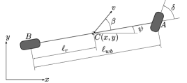
We use the kinematic bicycle model to model car-like robots, which captures their essential dynamics required for motion planning and control [24]. It effectively captures their nonholonomic constraints and has been demonstrated to be adequate in scenarios involving moderate acceleration [25, 26]. The model approximates the robots as a single-track model with two wheels, as depicted in Fig. 1.
The state vector is defined as
| (2) |
where and denote the global position coordinates, represents the heading (also called yaw angle), is the speed, and signifies the steering angle. The control input vector is given by , where denotes the acceleration, and represents the steering rate.
The dynamics of the kinematic bicycle model are defined by
| (3) |
where is the wheelbase of the vehicle, and the slip angle is defined as
| (4) |
with being the rear wheelbase.
II-B Control Barrier Functions
Control Barrier Functions provide a method to enforce safety constraints by ensuring that the system’s state remains within a safe set [1]. The safe set is defined as:
| (5) |
where is a continuously differentiable function. The time derivative of along the state trajectories is given by
which is the equivalent of the Lie derivative formalism
where and denote the Lie derivatives of along and , respectively.
Definition 1 (Control Barrier Function [27, 1]).
A continuously differentiable function is a Control Barrier Function for system 1 if there exists an extended class function such that
| (6) |
Definition 2 (Extended Class Function).
A function is said to be an extended class function if it is continuous, strictly increasing, and .
Definition 3 (Forward Invariant).
A set is forward invariant for the system 1 if its solutions starting at any initial satisfy .
Definition 4 (Relative Degree [28]).
We define
| (7) |
where denotes a th order differentiable class function and
| (8) |
with being a continuously differentiable function. We further define
| (9) |
Definition 5 (High-Order CBF [10, 11]).
Let and , be respectively defined by 7 and 9. A continuously differentiable function is a high-order CBF of relative degree for system 1 if there exist th order differentiable class functions and a class function such that
| (10) | ||||
where and denote Lie derivatives along and and one time(s), respectively, and encapsulates the remaining Lie derivatives along and partial derivatives w.r.t time with degree less than or equal to .
Theorem 1 ([11]).
Given a high-order CBF defined in Definition 5, then any Lipschitz continuous controller satisfying constraint 10 (or 11, equivalently) for all renders forward invariant for system 1.
III CBF with MTV-Based Safety Margin
In this section, we introduce a heading-aware safety margin based on the Minimum Translation Vector derived from the Separating Axis Theorem. We then describe how to approximate this safety margin using a neural network to ensure differentiability, allowing its integration into the CBF framework.
III-A MTV-Based Safety Margin
The Separating Axis Theorem (SAT) is a fundamental concept in computational geometry for detecting collisions between convex shapes [2]. SAT states that two convex shapes do not intersect if there exists an axis along which their projections do not overlap. If no such axis is found, the shapes are colliding. In this case, the Minimum Translation Vector represents the smallest vector required to separate the shapes, indicating the direction of least penetration and the minimum separation distance [3].
We extend the concept of MTV to define a heading-aware safety margin for two car-like robots modeled as rectangles. This safety margin represents the minimal movement required for one robot to collide the other, accounting for their orientations and positions.
We present Algorithm 1 to compute Minimum Translation Vector-based safety margin for a given pair of rectangles and by analyzing their projections on orthogonal axes. For each rectangle and each axis, it calculates the gap along that axis, determining if the projections overlap or are separated. Based on the signs of the gaps and , it classifies the relationship between the projections: non-overlapping, overlapping on one axis, or overlapping on both, and then computes a distance metric reflecting this relationship (lines 14 to 20). Using this metric, it classifies the rectangles as mutually separating, separating by one rectangle’s axes, or non-separating, and then computes the safety margin (lines 22 to 28).
The resulting safety margin accurately reflects the safety degree between two car-like robots, considering both positions and orientations. A positive value denotes the separation distance, while a negative value signifies collision, with its magnitude indicating the degree of penetration.
Remark 1.
The MTV-based safety margin computed by Algorithm 1 is non-differentiable due to operations such as minimum and maximum computations. This non-differentiability complicates integration with Control Barrier Functions and other control frameworks that require differentiable functions.
III-B Data-Driven Safety-Margin Predictor
To integrate the MTV-based safety margin with the CBF framework, we approximate the non-differentiable function presented in Algorithm 1 using a neural network, resulting in a differentiable safety-margin predictor.
Algorithm 1’s input includes the positions, orientations, widths, and lengths of two rectangles, creating a ten-dimensional input space in 2D Cartesian coordinates. To simplify learning, we reduce the input space using relative position and orientation, describing one rectangle from the perspective of the other. Assuming homogeneous robot geometries, the neural network can implicitly learn geometric dimensions without explicitly receiving them as inputs. We train a neural network , where denotes neural network parameters and represents its input, with as the relative position and as the relative heading of robot in the perspective of the ego robot .
III-C Relative Dynamics
Our safety-margin predictor works with relative positions and headings between two car-like robots and from the ego perspective of one robot. Without loss of generality, we designate robot as the ego robot. In this section, we define the relative dynamics of a system of two robots modeled by the kinematic bicycle model 3. We give the general form of the relative dynamics as
| (12) |
where and are locally Lipschitz, denotes the state vector, and is the joint action of robots and , with and as their respective control input vectors.
Since relative position and relative heading are expressed in the global coordinate system, we project them into robot ’s ego coordinate system, yielding
| (13) |
Applying the product rule to 13 gives us the first time derivative :
| (14) | ||||
Further, using the product rule to III-C yields the second time derivative :
| (15) | ||||
Similarly, we obtain the time derivatives of the relative state through the product rule:
| (16) |
where and denote the time derivatives of the state vectors of robots and in the global coordinate system, respectively, and and denote the corresponding relative time derivatives. We apply the equations of dynamics in 3 to compute and apply the product rule to it to compute as
| (17) |
where we compute with 4 and , with denoting the ratio of the rear wheelbase to the entire wheelbase and . Since all variables in 17 belong to robot , we omit the superscript to facilitate notations. The same computation applies to and for robot .
III-D Construction of the Control Barrier Function
We use the learned safety-margin predictor to construct a function accounting for the upper bound of the approximation error :
| (18) |
where we consider being time constant.
Assumption 1.
Function defined in 18 is continuously differentiable.
Remark 2.
Assumption 1 is mild since we can guarantee continuous differentiability by choosing a continuously differentiable activation function such as the TanH function within .
Proof.
Allowed by Assumption 1, we establish the relative degree by determining the number of times we must differentiate along the system dynamics 12 until any component of the control input explicitly appears.
First, the first time derivative of is
| (19) |
where denotes the gradient vector of w.r.t. , and recall that denotes the time derivative of the relative state vector in robot ’s ego perspective. Since depends on the state variables and their first derivatives, but not explicitly on the control input , the control input does not appear in .
Next, through the product rule, we yield the second time derivative of :
| (20) |
where is the Hessian matrix of . In , the control input and appear explicitly through as shown in III-C and 17.
Since the control input appears explicitly in the second derivative but not in the first derivative, has relative degree two. ∎
Note that we can easily compute the gradient vector in 19 and 20 and the Hessian matrix in 20 of the neural network since its parameters are known.
Corollary 1.
Assumption 2.
The upper bound of the approximation error in 18 is known.
Remark 3.
Assumption 2 is mild since we can estimate the upper bound of the approximation error by limiting the input space of to a known range, preventing out-of-distribution issues and allowing for a dense evaluation of all possible inputs. The input space is three-dimensional, containing the relative position and heading , where the latter is naturally bounded within [-, ]. We limit relative position to a small yet practical range around robot . We switch to Center-to-Center-based safety margin if robot falls outside this range, where conservatism has minimum impact.
Theorem 3.
Proof.
As per result of Theorem 4 of [10], is forward invariant for system 12, yielding that the system state will always stay within this set under the given controller in 22. As per definitions of in 9 and in 8, we have . As per definition of 18 and Assumption 2, the safety margin between robots and in the system will always be non-negative. Therefore, the system 12 will be collision-free forever. ∎
Remark 4.
Although the system defined in 12 contains only two robots, Theorem 3 applies to systems with any number of robots. For each robot pair, we construct a sub-system as in 2, resulting in sub-systems, where denotes the number of robots. The entire system remains collision-free as long as all sub-systems are collision-free.
III-E Optimal Control Problem Formulation
Consider a nominal controller, such as a learned-based controller, with the goal of ensuring safety. We formulate an Optimal Control Problem to verify the safety of this nominal controller. The objective is to find the minimum perturbation on the nominal control actions, denoted by , while satisfying safety and feasibility constraints. Formally, we formulate the Optimal Control Problem as:
| (23a) | ||||
| s.t. | (23b) | |||
| (23c) | ||||
| (23d) | ||||
where is a weighting matrix. Constraint 23c ensures collision-freeness, and Constraint 23d enforces feasibility of control actions within the system’s physical limits, where and represent the lower and upper bounds. We solve the Optimal Control Problem 23 repeatedly at each time step.
IV Experiments
We evaluate our proposed approach through numerical experiments in simulations involving two car-like robots in an overtaking scenario and a bypassing scenario, respectively. Codes reproducing our experimental results and video demonstrations are available at our open-source repository111github.com/bassamlab/sigmarl.
| Parameters | Values |
|---|---|
| Length , width | , |
| Wheelbase , rear wheelbase | , |
| Max. (min.) acceleration | () |
| Max. (min.) steering rate | () |
| Weighting matrix | (Identity matrix) |
For simplification, we use the same linear class functions for both : and , where is a positive coefficient. This yields constraint 23c to be .
In each scenario, we compare our proposed MTV-based safety margin with Center-to-Center-based safety margin. For the latter, we replace the CBF defined in 18 with the Center-to-Center-based distance:
| (24) |
where represents the minimum radius required to enclose the vehicle, with and being the vehicle’s length and width, respectively. 24 thus serves as a valid high-order CBF, allowing the use of 23.
We use an identity matrix as the weighting matrix in 23 for both the overtaking and bypassing scenarios without further tuning. Table I summarizes additional parameters used in both scenarios.
IV-A Preparation
IV-A1 Training the Safety-Margin Predictor
We generate a training dataset by computing the MTV-based safety margin using Algorithm 1. We limit robot ’s scope to and , with headings . The training dataset contains approximately 70k uniformly distributed data points. We train a simple fully connected neural network , with two hidden layers of 62 nodes each and TanH activation functions, to approximate the safety margin. We evaluate this network on a separate test dataset of 100k random data points within the state space. The maximum approximation error in our case is , corresponding to of the robot’s width, with the mean approximation error of just .
IV-A2 Nominal Controller
We use SigmaRL [29], an open-source multi-agent Reinforcement Learning framework for motion planning of Connected and Automated Vehicles, to train a nominal Reinforcement Learning policy. Henceforth, we will call the robots in the simulations vehicles. The nominal controller receives a short-term waypoint-based reference path at each time step and outputs control actions to follow it closely. We purposely train the policy to be greedy and disregard collision avoidance.
IV-A3 Integration with CBF
We integrate the learned safety-margin predictor within our high-order CBF with relative degree two. To optimize the greedy nominal Reinforcement Learning controller, we solve the Optimal Control Problem 23, a convex quadratic programming problem, using the package CVXPY [30, 31] for efficient convex optimization in Python.
IV-B Overtaking Scenario
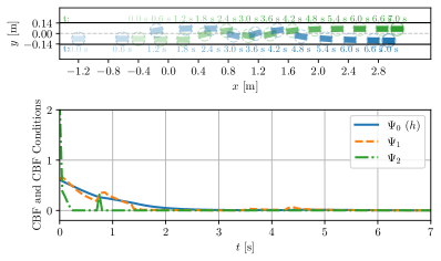
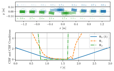
In this scenario, the blue ego vehicle attempts to overtake a green, slower-moving vehicle ahead. Vehicle employs a trained Reinforcement Learning nominal controller, which directs it to move at approximately , with our Control Barrier Function ensuring collision-freeness. In contrast, vehicle moves constantly at around with a slower Reinforcement Learning nominal controller and without a Control Barrier Function. To encourage overtaking, we manually project vehicle ’s reference path to the centerline of the adjacent lane. Additionally, to test our CBF’s robustness, vehicle conditionally switches lanes to obstruct vehicle ’s overtaking maneuver as it approaches. After obstructing three times, vehicle remains in its lane, ceasing interference with vehicle . Note that throughout the process, vehicle moves significantly slower than vehicle . We fine-tune the coefficient of the extended class functions, determining that is effective for both Center-to-Center- and Minimum Translation Vector-based safety margins.
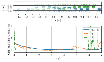
Results: Figure 2 depicts the performance of the Center-to-Center-based safety margin. Vehicle starts at and vehicle at . During the three obstructive maneuvers, the Center-to-Center-based safety margin successfully prevents a collision between vehicles and . After , per our setup, vehicle stops obstructing vehicle . However, vehicle cannot complete the overtake due to the conservatism of the Center-to-Center-based safety margin. The blue line in Fig. 2 depicts the value over time. Its near-zero values indicate that the system state is near the boundaries of , leaving no room for overtaking (otherwise, Eq. 23c would be violated). Conversely, as shown in Fig. 3, using our Minimum Translation Vector-based safety margin, vehicle successfully overtakes vehicle at .
IV-C Bypassing Scenario
In this scenario, two vehicles approach each other from opposite directions on a narrow road, where the road width allows for bypassing but requires precise maneuvering. Both vehicles use the same nominal Reinforcement Learning controller that instructs them to move at . We apply our CBF to both vehicles, optimizing their nominal control actions to guarantee collision-freeness. Let represent a horizontal line at . Initially, we project the nominal controllers’ reference points onto the horizontal lines and . As they approach, we project to and to encourage bypassing. We jointly tune and for optimal bypassing with minimal . Final values are ( of the vehicle width) and for Center-to-Center-based safety margin, and ( of the vehicle width) and for Minimum Translation Vector-based safety margin.
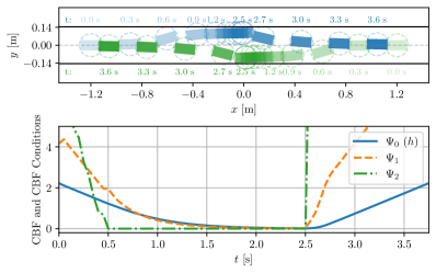
Results: As shown in Fig. 4, vehicle starts at moving rightward and vehicle at moving leftward. At , they have the smallest safety margin and successfully bypass each other, but with excessive evasion: the maximum lateral evasion of vehicle is of the vehicle width and that of vehicle is , averaging to . The total bypassing time is about . In comparison, using our Minimum Translation Vector-based safety margin, at , they have the smallest safety margin and successfully bypass each other afterward. The average evasion of both vehicles is only of the vehicle width— less than the Center-to-Center-based safety margin. Besides, the bypass process completes at , faster than the Center-to-Center-based safety margin.
IV-D Discussions and Limitations
The overtaking and bypassing scenarios demonstrate the superior performance of our MTV-based safety margin as a CBF for safety verification. In the overtaking scenario, the traditional C2C-based margin fails, whereas the MTV-based margin enables smooth, safe, and efficient overtaking. In the bypassing scenario, while both margins succeed, the MTV-based margin reduces lateral space usage by nd time by compared to the C2C-based margin. Importantly, this performance improvement does not increase computation time: in the overtaking scenario, solving the Optimal Control Problem 23 requires an average of per step with the Center-to-Center-based safety margins and with the Minimum Translation Vector-based safety margins, while in the bypassing scenario, it takes and , respectively. Therefore, our method mitigates the excessive conservatism of traditional approaches without introducing extra computation burden.
Applying our high-order CBF requires computing the gradient and Hessian matrix of the safety margin predictor (see 19 and 20). However, the exact approximation error remains unknown, as the original function for the MTV-based margin is non-differentiable, preventing us from computing their actual values. Nevertheless, given the marginal approximation error in the safety margin ( of robot’s width on average) and its continuity nature, we expect the gradient and Hessian approximation errors to be similarly minor and negligible.
V Conclusions
We proposed a learning-based Control Barrier Function with a heading-aware safety margin to reduce conservatism in collision avoidance for car-like robots. By incorporating the robots’ orientations and true geometries, our method offers a more precise estimation of safe regions. To ensure differentiability required by Control Barrier Functions, we approximated the non-differentiable safety margin function using a neural network. We showed that our Minimum Translation Vector-based safety margin is a high-order Control Barrier Function with relative degree two for a system with two robots modeled by the nonlinear kinematic bicycle model. By incorporating the upper bound of the approximation error into the CBF conditions, we formally guaranteed safety through forward invariance. Experiments with two Connected and Automated Vehicles in overtaking and bypassing scenarios demonstrated that our approach reduces conservatism significantly compared to traditional Center-to-Center-based safety margin while ensuring safety.
References
- [1] A. D. Ames, X. Xu, J. W. Grizzle, and P. Tabuada, “Control barrier function based quadratic programs for safety critical systems,” IEEE Transactions on Automatic Control, vol. 62, no. 8, pp. 3861–3876, 2017.
- [2] S. Gottschalk, M. C. Lin, and D. Manocha, “OBBTree: A hierarchical structure for rapid interference detection,” in Proceedings of the 23rd annual conference on Computer graphics and interactive techniques, 1996, pp. 171–180.
- [3] C. Ericson, Real-time collision detection. Crc Press, 2004.
- [4] J. Ji, A. Khajepour, W. W. Melek, and Y. Huang, “Path planning and tracking for vehicle collision avoidance based on model predictive control with multiconstraints,” IEEE Transactions on Vehicular Technology, vol. 66, no. 2, pp. 952–964, 2016.
- [5] S. Magdici and M. Althoff, “Fail-safe motion planning of autonomous vehicles,” in 2016 IEEE 19th International Conference on Intelligent Transportation Systems (ITSC). IEEE, 2016, pp. 452–458.
- [6] P. Scheffe, M. V. A. Pedrosa, K. Flaßkamp, and B. Alrifaee, “Receding horizon control using graph search for multi-agent trajectory planning,” IEEE Transactions on Control Systems Technology, vol. 31, no. 3, pp. 1092–1105, 2023.
- [7] P. Scheffe, T. M. Henneken, M. Kloock, and B. Alrifaee, “Sequential convex programming methods for real-time optimal trajectory planning in autonomous vehicle racing,” IEEE Transactions on Intelligent Vehicles, vol. 8, no. 1, pp. 661–672, 2023.
- [8] Y. Chen, H. Peng, and J. Grizzle, “Obstacle avoidance for low-speed autonomous vehicles with barrier function,” IEEE Transactions on Control Systems Technology, vol. 26, no. 1, pp. 194–206, 2017.
- [9] L. Wang, A. D. Ames, and M. Egerstedt, “Safety barrier certificates for collisions-free multirobot systems,” IEEE Transactions on Robotics, vol. 33, no. 3, pp. 661–674, 2017.
- [10] W. Xiao and C. Belta, “Control barrier functions for systems with high relative degree,” in 2019 IEEE 58th Conference on Decision and Control (CDC), 2019, pp. 474–479.
- [11] W. Xiao, T.-H. Wang, R. Hasani, M. Chahine, A. Amini, X. Li, and D. Rus, “BarrierNet: Differentiable control barrier functions for learning of safe robot control,” IEEE Transactions on Robotics, vol. 39, no. 3, pp. 2289–2307, 2023.
- [12] Z. Zhang, S. Han, J. Wang, and F. Miao, “Spatial-temporal-aware safe multi-agent reinforcement learning of connected autonomous vehicles in challenging scenarios,” in 2023 IEEE International Conference on Robotics and Automation (ICRA), 2023, pp. 5574–5580.
- [13] S. Han, S. Zhou, J. Wang, L. Pepin, C. Ding, J. Fu, and F. Miao, “A multi-agent reinforcement learning approach for safe and efficient behavior planning of connected autonomous vehicles,” IEEE Transactions on Intelligent Transportation Systems, vol. 25, no. 5, pp. 3654–3670, 2024.
- [14] Y. Chen, A. Singletary, and A. D. Ames, “Guaranteed obstacle avoidance for multi-robot operations with limited actuation: A control barrier function approach,” IEEE Control Systems Letters, vol. 5, no. 1, pp. 127–132, 2020.
- [15] A. Singletary, K. Klingebiel, J. Bourne, A. Browning, P. Tokumaru, and A. Ames, “Comparative analysis of control barrier functions and artificial potential fields for obstacle avoidance,” in 2021 IEEE/RSJ International Conference on Intelligent Robots and Systems (IROS). IEEE, 2021, pp. 8129–8136.
- [16] Z. Gao, G. Yang, and A. Prorok, “Online control barrier functions for decentralized multi-agent navigation,” in 2023 International Symposium on Multi-Robot and Multi-Agent Systems (MRS). IEEE, 2023, pp. 107–113.
- [17] E. Rimon and S. P. Boyd, “Obstacle collision detection using best ellipsoid fit,” Journal of Intelligent and Robotic Systems, vol. 18, no. 2, pp. 105–126, 1997.
- [18] C. K. Verginis and D. V. Dimarogonas, “Closed-form barrier functions for multi-agent ellipsoidal systems with uncertain lagrangian dynamics,” IEEE Control Systems Letters, vol. 3, no. 3, pp. 727–732, 2019.
- [19] H. Tanner, S. Loizou, and K. Kyriakopoulos, “Nonholonomic navigation and control of cooperating mobile manipulators,” IEEE Transactions on Robotics and Automation, vol. 19, no. 1, pp. 53–64, 2003.
- [20] C. K. Verginis and D. V. Dimarogonas, “Multi-agent motion planning and object transportation under high level goals*,” IFAC-PapersOnLine, vol. 50, no. 1, pp. 15 816–15 821, 2017.
- [21] W. Schwarting, J. Alonso-Mora, L. Paull, S. Karaman, and D. Rus, “Safe nonlinear trajectory generation for parallel autonomy with a dynamic vehicle model,” IEEE Transactions on Intelligent Transportation Systems, vol. 19, no. 9, pp. 2994–3008, 2018.
- [22] Z. Jian, Z. Yan, X. Lei, Z. Lu, B. Lan, X. Wang, and B. Liang, “Dynamic control barrier function-based model predictive control to safety-critical obstacle-avoidance of mobile robot,” in 2023 IEEE International Conference on Robotics and Automation (ICRA), 2023, pp. 3679–3685.
- [23] H. Liu, Z. Huang, Z. Zhu, Y. Li, S. Shen, and J. Ma, “Improved consensus admm for cooperative motion planning of large-scale connected autonomous vehicles with limited communication,” IEEE Transactions on Intelligent Vehicles, pp. 1–17, 2024.
- [24] R. Rajamani, Vehicle dynamics and control. Springer Science & Business Media, 2011.
- [25] P. Polack, F. Altché, B. d’Andréa Novel, and A. de La Fortelle, “The kinematic bicycle model: A consistent model for planning feasible trajectories for autonomous vehicles?” in 2017 IEEE intelligent vehicles symposium (IV). IEEE, 2017, pp. 812–818.
- [26] A. B. Ghosn, P. Polack, and A. de La Fortelle, “The hybrid extended bicycle: A simple model for high dynamic vehicle trajectory planning,” in 2024 IEEE 27th International Conference on Intelligent Transportation Systems (ITSC), in press. IEEE, 2024.
- [27] A. D. Ames, J. W. Grizzle, and P. Tabuada, “Control barrier function based quadratic programs with application to adaptive cruise control,” in 53rd IEEE Conference on Decision and Control, 2014, pp. 6271–6278.
- [28] H. Khalil, “Nonlinear systems,” 2002.
- [29] J. Xu, P. Hu, and B. Alrifaee, “SigmaRL: A sample-efficient and generalizable multi-agent reinforcement learning framework for motion planning,” in 2024 IEEE 27th International Conference on Intelligent Transportation Systems (ITSC), in press. IEEE, 2024.
- [30] S. Diamond and S. Boyd, “CVXPY: A Python-embedded modeling language for convex optimization,” Journal of Machine Learning Research, vol. 17, no. 83, pp. 1–5, 2016.
- [31] A. Agrawal, R. Verschueren, S. Diamond, and S. Boyd, “A rewriting system for convex optimization problems,” Journal of Control and Decision, vol. 5, no. 1, pp. 42–60, 2018.
- [32] J. Xu, O. Sobhy, and B. Alrifaee, “XP-MARL: Auxiliary prioritization in multi-agent reinforcement learning to address non-stationarity,” arXiv preprint, 2024.