Microfoundation Inference for Strategic Prediction
Abstract
Often in prediction tasks, the predictive model itself can influence the distribution of the target variable, a phenomenon termed performative prediction. Generally, this influence stems from strategic actions taken by stakeholders with a vested interest in predictive models. A key challenge that hinders the widespread adaptation of performative prediction in machine learning is that practitioners are generally unaware of the social impacts of their predictions. To address this gap, we propose a methodology for learning the distribution map that encapsulates the long-term impacts of predictive models on the population. Specifically, we model agents’ responses as a cost-adjusted utility maximization problem and propose estimates for said cost. Our approach leverages optimal transport to align pre-model exposure (ex ante) and post-model exposure (ex post) distributions. We provide a rate of convergence for this proposed estimate and assess its quality through empirical demonstrations on a credit-scoring dataset.111Code: https://github.com/felipemaiapolo/microfoundation_inference.
1 Introduction
Consider a supervised learning scenario where the predictive model triggers actions that alter the target distribution, thereby impacting its own performance. This scenario is referred to as performative prediction (Perdomo et al., 2020) and is prevalent in social prediction contexts, where predictions influence (strategic) individuals. For example, traffic forecasts affect traffic patterns, crime location predictions influence police deployment that may deter crime, and stock price predictions drive trading activity, consequently affecting prices. Campbell’s law (Campbell, 1979), which states that
The more any quantitative social indicator is used for social decision-making, the more subject it will be to corruption pressures and the more apt it will be to distort and corrupt the social processes it is intended to monitor.
acknowledges the ubiquity of performativity in social prediction problems.
The learner may respond to this performative distribution shift by frequently retraining the model with new data, but this approach is often impractical, as Perdomo et al. (2020) describes this as a “cat and mouse game of chasing a moving target.” They suggest a more structured approach, framing risk minimization under performativity within a decision-theoretic framework to find equilibria where the model is optimal for the distribution it creates. This idea was also explored by Hardt et al. (2016) in strategic classification, a notable subtype of performative prediction. Subsequent research has focused on computing performative stable (Mendler-Dünner et al., 2020) or performative optimal (Izzo et al., 2022) policies and developing related algorithms for online settings (Jagadeesan et al., 2022). For a more detailed review of the literature, see Section 1.1.
In performative prediction, the specific mechanism of the distribution shift is usually unknown. Previous work circumvents this issue in two ways: The first is to treat the performative prediction problem (2.2) as a zeroth order (derivative-free) optimization problem, where one only relies on samples drawn from the distributions induced by iterations and solves the performative prediction problem without knowing the performative distribution map , i.e. the map of performative distribution induced by a predictor (Izzo et al., 2021; Miller et al., 2021). One drawback of this approach is its slow convergence: e.g. Izzo et al.’s algorithm relies on finite differences to approximate the gradient of the performative risk, so it suffers from the curse of dimensionality.
The second approach stipulates that each agent follows a (potentially misspecified) microfoundation model (Jang et al., 2022) and incorporates the anticipated agent responses into the optimization. This method leverages the fast convergence rates of the algorithm for performative risk minimization that benefit from full access to the distribution map (Hardt et al., 2016; Levanon and Rosenfeld, 2021; Cutler et al., 2021; Somerstep et al., 2023). However, the agent response model is often inaccurate (Lin and Zrnic, 2023), leading to incorrect distribution maps and preventing effective resolution of the performative prediction problem. We illustrate this issue in an example of strategic ordinary least squares (OLS) prediction in Example 2.1.
To address this issue, we propose an estimator for the microfoundation models of agent responses. Our approach complements the second approach; on the one hand, we alleviate the issues of misspecified agent response models by learning the microfoundations model from agent response data, and on the other hand, the white-box access to the distribution map allows the learner to take advantage of faster optimization algorithms for minimizing the performative risk. Another benefit of our approach is that it is well suited to more sophisticated learning algorithms (e.g. algorithms that enforce constraints (Maity et al., 2021; Somerstep et al., 2023)) that have no obvious zeroth order counterpart.
Our approach to estimate the microfoundation model is to assume that the agents’ microfoundation is a utility maximization problem consisting of a (model-dependent) known benefit function and an unknown cost function . A detailed exposition of our approach can be found in Section 3, where we develop an optimal transport-based method to estimate the cost within a class of Bregman divergences. Our contributions are as follows:
-
1.
We propose a method for estimating the cost function (within a class of Bregman divergences) of a general utility-maximizing microfoundation model. Our method relies on matching pre-model deployment and post-model deployment distributions with optimal transport.
-
2.
We provide an analysis of identifiability in the estimation of the cost function, as well as rates of convergence of our proposed estimator.
-
3.
We perform numerical experiments that both exhibit the performance of our methodology in estimating the cost and demonstrate its usefulness on a variety of down-stream tasks. We also demonstrate empirically that our methodology satisfies certain robustness properties with respect to misspecification of the benefit function.
1.1 Related works
The performative prediction problem was introduced by Perdomo et al. (2020). Much of the methodological focus in performative prediction is on locating performative stable or performative optimal solutions. To locate a stable solution, a paradigm of repeated retraining has been developed in multiple environments Mendler-Dünner et al. (2020); Drusvyatskiy and Xiao (2023). Furthermore, a line of prior work on this often utilizes zero’th order algorithms such as finite differences Izzo et al. (2021, 2022) or regret minimization (Jagadeesan et al., 2022; Dong et al., 2018; Chen et al., 2020). Other works instead assume white-box access to a pre-specified performative map (Levanon and Rosenfeld, 2021; Somerstep et al., 2023; Shavit et al., 2020; Lin and Zrnic, 2023). Finally, others make structural assumptions on the underlying data (e.g assuming all data is drawn from a location-scale family) (Miller et al., 2021). As pointed out in Lin and Zrnic (2023) such pre-specified maps are often misspecified leading to erroneous results. We focus on correcting this by building a robust method to infer performative maps.
Originating with strategic classification Hardt et al. (2016); pre-specified models of performative maps are often at the sample level, and correspond to samples behaving as agents with strategic behavior. Strategic classification has been expanded in several directions: including models with causality Mendler-Dünner et al. (2022); Horowitz and Rosenfeld (2023); Somerstep et al. (2023); Harris et al. (2022), models with opaque agent behavior Ghalme et al. (2021), the effects of strategic behavior on graph neural networks Eilat et al. (2023), models with reversed order of play Zrnic et al. (2022), PAC learning for strategic classification Sundaram et al. (2021), strategic ordinary least squares Shavit et al. (2020) and combinations of these (Levanon and Rosenfeld, 2022). Strategic behavior with an element of competition between agents has been used to model the behavior of content creators in socio-technical systems (Hron et al., 2023; Jagadeesan et al., 2023). The study of strategic behavior is not isolated to computer science; strategic behavior is the key ingredient to many micro-economic models of labor markets (Coate and Loury, 1993; Moro and Norman, 2003, 2004; Fang and Moro, 2011).
The common theme of strategic behavior is that each data sample is an agent that is assumed to maximize a cost-adjusted utility that depends on the model ; therefore, the performative map is implicitly determined by the agents’ utility and cost. Our main contribution is a methodology that allows practitioners to infer agents’ costs and utilities. Prior work on inferring performative maps is relatively light. The works of Mendler-Dünner et al. (2022); Lechner et al. (2023) assume that the aggregate manipulation structure is in a class of graphs and infer the manipulation graph. Shavit et al. (2020) includes some focus on the inference of strategic responses, but only in the case of linear regression. Our methodology is applicable beyond these special cases and additionally allows for inference with both samples from the ex-ante and an ex-post distribution or samples from multiple ex-post distributions.
Inference of agent costs and utilities is often a crucial step in deploying accurate models in performative settings. For example, utilizing differentiable proxies to , the authors of Levanon and Rosenfeld (2021) provide a framework for minimizing performative risk in a strategic environment. Unfortunately, if the strategic model is not specified correctly, then the resulting estimator of an optimal model will not be consistent (Lin and Zrnic, 2023). Our methodology allows for practitioners to utilize plug-in optimization frameworks with peace of mind.
2 Microfoundations for strategic prediction
We follow the performative prediction setting in (Perdomo et al., 2020, Section 5): at the microlevel, the agents are rational, i.e. they respond to a predictive model by choosing their best actions. Each agent is represented by a pair of attributes , where and are the covariates and the outcome of an individual. Before agents are exposed to a model their attributes follow an ex-ante distribution (where is the set of probability measures over ), and, having been exposed to , they strategically maximize their cost-adjusted utility that depends on ; i.e. in response to each agent updates their individual via
| (2.1) |
Here, encodes the benefit of the agent changing their attributes to when exposed to , and is a cost function that encodes the burden of changing their attributes from to . Throughout, we will assume that is known, and remains to be estimated. Often, the utility is simply the output of the learners predictive model (e.g. in standard strategic classification (Hardt et al., 2016)) or is a function of a learner controlled wage and output of the learners predictive model (e.g. in labor market models (Coate and Loury, 1993)). In either case, all information pertinent to the benefit function is known to the learner, which is why we focus on the case of known benefit functions and unknown costs. Additionally, we will demonstrate (cf. Sections 5 & Appendix B) that our methodology correctly estimates even if is misspecified, (though the cost will not be estimated correctly).
We call the agents’ response map. Due to the agents response to , the distribution of attributes has now shifted to , which is the push-forward measure of through the agents’ response . We refer to this as the performative distribution or ex-post distribution under the learner’s action . The map is referred to as the performative distribution map or simply distribution map.
The microfoundation model in eq. (2.1) covers a variety of performative prediction problems, that includes strategic classification (Hardt et al., 2016), causal strategic classification (Miller et al., 2020; Levanon and Rosenfeld, 2021; Shavit et al., 2020; Somerstep et al., 2023), content creation (Hron et al., 2022), and micro-economic models of labor markets (Coate and Loury, 1993).
2.1 Importance of microfoundation inference for downstream tasks
Next, we cover two important use cases for estimating the agents microfoundations.
Performative risk minimization As a response to the distribution shift, the learner aims to learn a predictor that minimizes the performative risk which accounts for the agents’ response:
| (2.2) |
where is the appropriate prediction loss. Previous methods for performative risk minimization incorporate an agents’ microfoundation to anticipate the distribution shift (Hardt et al., 2016; Levanon and Rosenfeld, 2021; Somerstep et al., 2023). As we demonstrate in the following example, estimates obtained using a misspecified microfoundation can be arbitrarily poor.
Example 2.1 (Causal Strategic OLS (Shavit et al., 2020)).
In a linear regression setting, we highlight the importance of estimating the cost. Consider an ex-ante distribution of agents’ profiles, where a typical sample point satisfies the following: and for an the , for a . Once a is published, agents adjust their ’s to maximize their benefit , while the ’s remain unchanged. Assuming that the true cost is , where is a predetermined positive definite matrix, the true agent’s response map and performative risk are
| (2.3) |
| (2.4) |
If the agents cost is misspecified to , then by letting in the equations (2.3) and (2.4) the learner anticipates the agents map and the corresponding performative risk as
| (2.5) |
As we show in Lemma A.1 that the learner who minimizes the wrongly anticipated decides on its optimizer where is the only positive solution to equation . However, the true performance risk for such a is suboptimal, since
| PR |
can be arbitrarily large depending on , and, even trivially predicting every response as has a better performative risk than . To mitigate this suboptimality, one must estimate the cost.
Enforcing long-term fairness: Beyond accuracy, the call for practitioners to deploy socially responsible models in performative settings has grown; models are generally considered socially responsible if they either induce improvement (encourage increase of agent outcomes ) or treat agents fairly post distribution shift (Miller et al., 2020; D’Amour et al., 2020; Estornell et al., 2021; Liu et al., 2018; Somerstep et al., 2024). In either case, if one wishes to meet some definition of responsibility, inference on the individuals’ response to models (e.g the cost for an individual to improve in response to ) is a necessary step.
3 Learning agents’ response
The first sticking point in agent cost estimation is a question identifiability: what class of costs can be learned if one only observes a finite number of samples over a finite number of model deployments? Note that estimating a general bivariate cost function is conceptually impossible when we have access to samples from only finitely many ex-post distributions , in addition to the ex-ante distribution ; even if we assume that we know the exact distributions. From the equality , we can only know the finite number of actions by the agent with the ex-ante attribute when exposed to the models . Thus, from the first-order condition of (2.1), which is
one can only evaluate the partial derivative of the cost at the points and for a given it is impossible to evaluate beyond these points.
3.1 Agents’ cost as Bregman Divergence
In light of the non-identifiability of the generic cost from a finite number of ex-ante distributions, we estimate the agents’ cost within a class of Bregman divergences (Bregman, 1967):
where is a strictly convex Bregman potential. This assumption mitigates the problem of non-identifiability of the cost for finitely many deployed models , because estimating is reduced to estimating , thus eliminating the joint dependency of . In addition to making it possible to estimate the cost function, the Bregman divergence specification allows us to set the problem of cost estimation in an optimal transport framework. Furthermore, the class of Bregman divergences is broad and often subsumes classes of costs that are studied in other works. For example: Perdomo et al., 2020, Section 5.2, Hardt et al., 2016, Section 5.1 considers a simple cost, which is a special case of Bregman divergence with potential ; in Liu et al. (2023) the cost is for some positive definite matrix , which is a special case of Bregman divergence with potential ; Other parametric restrictions imposed on distribution maps in the strategic learning literature include Izzo et al. (2021); Miller et al. (2021); Jagadeesan et al. (2022).
As the divergence is induced by its potential , from now on we focus on estimating . We consider two scenarios depending on whether a sample from the ex-ante distribution is available or not.
3.2 Learning from ex-ante and ex-post distributions
First, we assume that the learner has random samples from the ex ante distribution and from ex-post distributions related to the agents’ response to prediction models . Let and ’s be the empirical counterparts of and ’s. We estimate by solving
| (3.1) | ||||
a class of convex potential functions, the 2-Wasserstein distance and denotes the push-forward measure of through the map .
The problem (3.1) is motivated by a first-order characterization of the micro-level responses in (2.1); for a generic :
| (3.2) | |||
where is the (unknown) Bregman potential for the cost. We recall that , which implies the distributions and must be identical:
where denotes equality in distributions. It follows that for , , , are all identically distributed. In optimization (3.1) we estimate by exploiting this equality in the distribution, where we minimize the 2-Wasserstein variance. We use the (2-)Wasserstein distance in (3.1) because agent responses may not have common support, and it also allows us to leverage algorithms for fast computation of Wasserstein barycenters to solve (3.1) in a block coordinate descent algorithm. We summarize our method in Algorithm 1.
| (3.3) |
Although it is often desirable to estimate the nonparametrically, for a higher dimensional one may further restrict to a suitable parametric class of potential functions and find the optimal within that class. We provide an example of such a parametric specification in Section 5.2, where we assume that the cost function is quadratic, i.e. for a positive definite , in which case the potentials are parameterized as .
3.3 Learning from ex-post distributions
Assume that only observations of the ex post (performative) distributions ’s are available. Similarly to before, the first-order optimality conditions of the (2.1) show that the push-forwards of the agent responses under , are identical, which suggests we estimate aligning the pushforward distributions of the agent responses under the ’s:
| (3.4) | ||||
4 Theoretical analysis
Identifiability of the cost function:
A crucial step in analyzing the estimated cost is to verify whether it is identifiable from the proposed algorithms. More specifically, we investigate whether the potential functions obtained from (3.1) and (3.4) induce a Bergman divergence identical to (the true cost function), when the empirical distributions are substituted by their respective population versions . Since a Bergman divergence remains identical under any linear adjustment to its inducing potential, we verify whether contains
| (4.1) |
To verify this, we first observe that the objectives of (4.1) are identical to zero when , as we argue after (3.1) that , are identically distributed. Since these objectives are non-negative, it is clear that they must be zero at their minimum value, which further implies that for any minimizer , all distributions used to calculate the barycenter distances must be identical to the barycenters. In the following lemma, we make use of this observation to derive an equivalence condition to verify whether the cost is identifiable.
Theorem 4.1.
In the ex-ante problem, denote the transportation maps from the barycenter to the measures as , and similarly, in (ex-post), denote them as . Then an equivalent condition for (4.1) is that all conservative solutions (i.e. can be written as the derivative of a convex function) of the following equations are constant functions.
| (4.2) |
In practice, this condition can be used to verify whether the cost is uniquely identified from the available dataset. As an example, consider the following corollary.
Corollary 4.2.
With access to the ex-ante distribution assume that only one performative distribution is observed. If is strictly concave with a finite maximizer, then the condition in Theorem 4.1 is satisfied. Thus, the cost function is identified only from these two distributions.
Rate of convergence for cost estimation:
In addition to identifiability, we also establish a convergence rate for our proposed estimator using two distributions. Specifically, we estimate within a parametric class using samples from two distributions: an ex-ante () and a single ex-post (). In this case, the loss utilized to estimate in Algorithm 1 is
| (4.3) |
and the population value () and the estimated value () of the parameter can be calculated as
where and are the empirical counterparts of and , and is the set of probability measures on with marginals and . In the following theorem, we establish an convergence rate between and in the case where the OT loss used for cost estimation satisfies a strong convexity assumption. Note that this strong convexity assumption implies that we are also assuming that the cost is identifiable.
Theorem 4.3.
Suppose that and are compactly supported on and are absolutely continuous with respect to the Lebesgue measure with bounded second moments. Denote and as their empirical counterparts, each calculated using samples. Furthermore, assume that both and are strongly convex. Then there exists a such that
| (4.4) |
This rate was established using convergence results for the empirical Wasserstein distance from Manole and Niles-Weed (2024, Theorem 2). Extending the upper bound in (4.4) to multiple ex-post distributions or to nonidentical sample sizes for ex-ante and ex-post distributions is possible, but, to the best of our knowledge, similar convergence results for the empirical Wasserstein distance that we may require are not available in the literature and we leave this for future work.
Impact of estimated the cost.
Having estimated the , we can plug it in eq. (3.2) and estimate the response map from the equation
| (4.5) |
which is then used in the performative loss function to estimate the performative optimal (PO) solution:
| (4.6) |
To understand the comparison of against the we recall the analysis in Lin and Zrnic (2023); especially Theorem 2. They decompose the risk-difference as
| (4.7) |
The first term is the error due to misspecification in our performative response map, often depending on the problem at hand and users’ choice of the class of potential functions. The second term is a statistical error in estimating this response map. For a parametric specification of we establish a rate of convergence for the said parameters (cf. Theorem 4.3). Under standard regularity conditions (e.g. smoothness of the loss function and response map) one can understand that the statistical error will have the same rate of convergence.
5 Experiments
In this section, we demonstrate the effectiveness, robustness, and competitiveness of our method in semi-synthetic setups. We use real data distributions as the ex-ante distributions and simulate agents’ strategic behavior as utility-maximizing, consistent with (2.1).
Dataset: We use the same credit scoring dataset from Perdomo et al. (2020), which is publicly available on Kaggle (Cukierski, 2011). The performative prediction framework is particularly relevant in the credit scoring context, as individuals may face restricted access to credit once a predictive model is deployed by a credit bureau. To counter these constraints, agents adapt their behavior to manipulate the system after a credit predictor is introduced. In this dataset, the target variable is a default indicator (), equal to one if an individual is 90 days delinquent or worse, and zero otherwise. Explanatory variables include metrics such as the total balance on credit cards and personal lines of credit, divided by the total credit limits ().
5.1 Estimating and
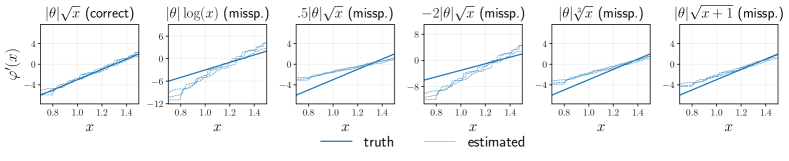
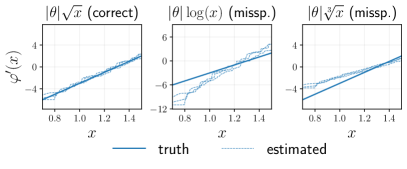
In this subsection, we demonstrate the performance of our method to estimate and using both ex-ante and ex-post distributions when the benefit function is known. To estimate in the uni-dimensional case with one ex-ante distribution and one ex-post distribution, we use a non-parametric estimator for . Specifically, is estimated via monotonic (isotonic) regression and subsequently integrated to estimate . Since RevolvingUtilizationOfUnsecuredLines has the highest marginal correlation with the target and is manipulable by agents, we focus on this feature. We first correctly specify as and then consider two cases of misspecification for : and . Results for additional types of misspecification are presented in Appendix C.2. The predictor is obtained by fitting a logistic regression that predicts from . This analysis helps us assess the robustness of our method in the presence of misspecification in the benefit function.
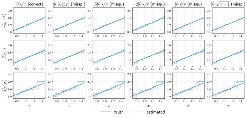
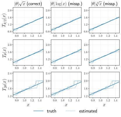
We begin by evaluating the accuracy of our method in estimating when samples from each of the two distributions are available. From Figure 1, we observe that the estimated functions are close to the true one when the benefit is correctly specified. However, the estimates exhibit significant bias when the benefit is misspecified. Despite this, Figure 2 shows that this bias does not carry over to the estimates of . Intuitively, this occurs because the misspecification of the benefit function is absorbed during the estimation of (thereby compromising its accuracy) but does not affect the overall predictive performance of the method. In Figure 2, we estimate for different values of and assess whether this robustness persists even when attempting to estimate the map for values of different from those used to induce the ex-post distribution and estimate , i.e., . An interesting pattern observed in Figure 2 is that the estimates deteriorate as increases in ; this occurs because samples are transported over greater distances to regions of the space where data points are sparse, leading to noisier estimates. For both figures, we report estimates based on different random seeds.
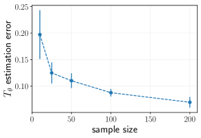
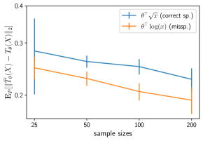
Finally, we show how the estimation error for behaves with different sample sizes when the is correctly specified. We assume that the number of data points in each one of the distributions is and consider the estimation error to be where denotes the support of our observations, which is fixed through sample sizes. Figure 4 shows that the estimation error of our method decreases as the sample size grows. The dots give the average error, and the error bars the standard deviation across random seeds.
5.2 Minimizing the performative risk
In this subsection, we apply our method to minimize the performative risk. We work in a multidimensional setup in which is composed of RevolvingUtilizationOfUnsecuredLines, DebtRatio (monthly debt payments divided by monthly gross income), Monthly income, and a constant representing the intercept. To simplify things, we consider all the features in to be performative and assume a linear benefit with a quadratic cost structure as in Example 2.1. To obtain ex-ante and ex-post data we publish a set of classifiers randomly sampled from a Gaussian distribution centered around the optimal classifier in the ex-ante distribution . We then estimate using Algorithm 1 where the minimization step over the set of all matrices is done using the Cholesky decomposition by optimizing for over the set of lower triangular matrices. Once the map is estimated, we obtain a plugin estimator (4.6) for a logistic regression by minimizing the cross-entropy loss. More details are in Appendix C.1.
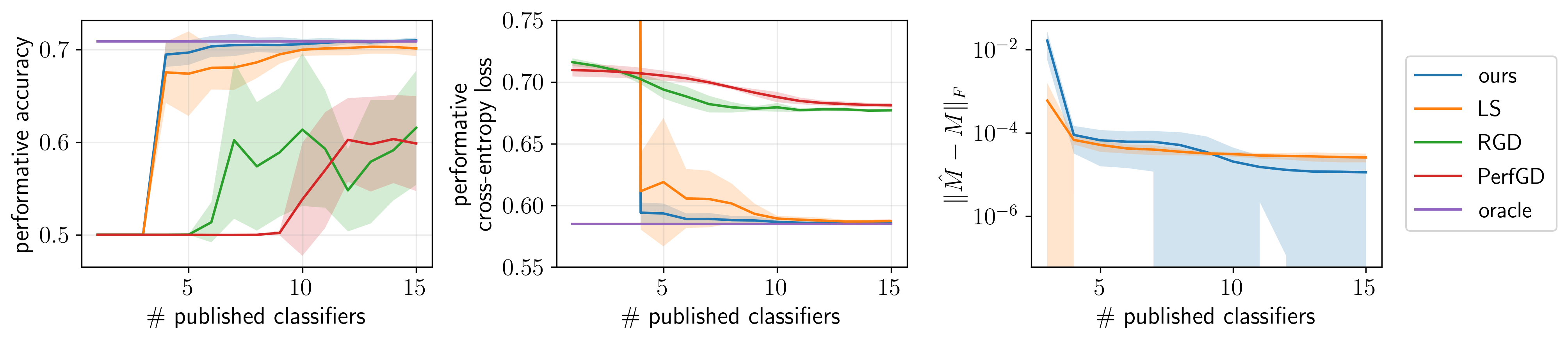
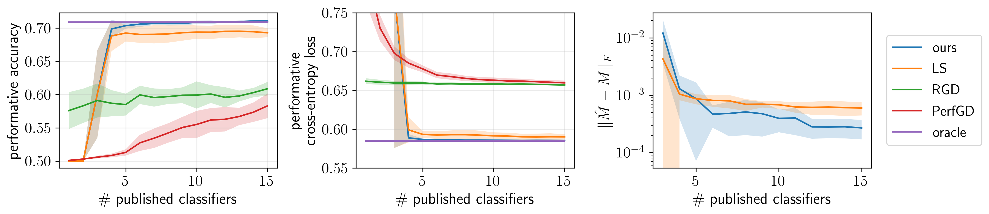
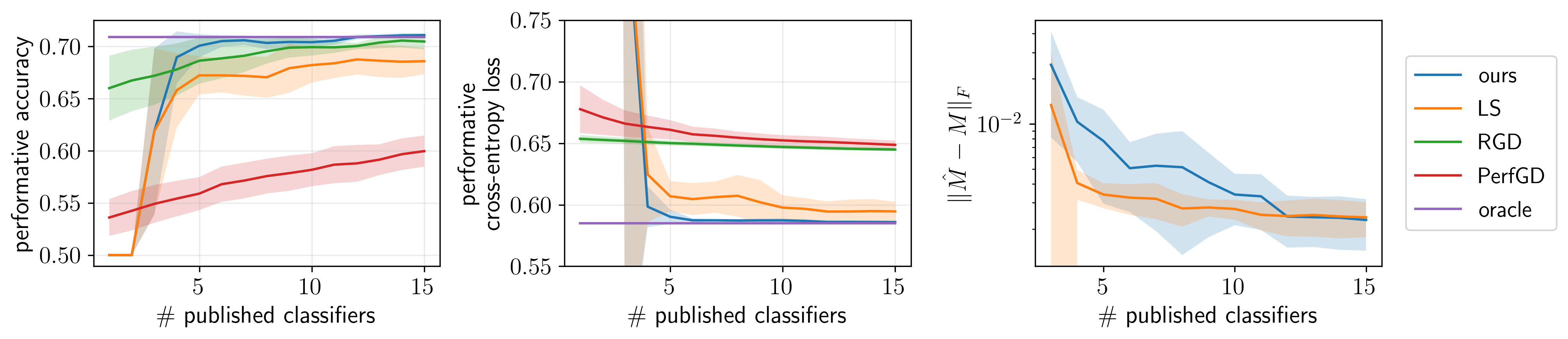
We compare our method with four baselines: (1) oracle, the classifier that uses the true performative map to minimize performative cross-entropy loss in the test dataset; (2) Repeated Gradient Descent (RGD) (Perdomo et al., 2020); (3) Performative Gradient Descent (PerfGD) (Izzo et al., 2022); and (4) the two-step method proposed by Miller et al. (2021) which includes least-squares estimator for the matrix , also used by Jagadeesan et al. (2022, Algorithm 2). We call the last method LS. For RGD and PerfGD, we ran experiments with different learning rates and selected those maximizing performative accuracy after the last classifier was published. For PerfGD, we assume that the induced distributions are Gaussian with a known mean structure (as it depends on ), a known covariance, and a known derivative of its mean with respect to222In equation 4 of Izzo et al. (2022). .
The left and middle plots in Figure 3 present the test set accuracies and cross-entropy losses across various classification strategies as the number of published classifiers increases. The right plot illustrates a comparison between our estimator for and the least squares approach from Miller et al. (2021). In all cases, our method demonstrates competitive performance relative to the baselines. Two additional observations are noteworthy. First, despite our implementations of RGD and PerfGD being optimized for those methods, their performance can be suboptimal in several scenarios, as shown in Figure 3 and Appendix C.2. The Gaussianity assumption inherent in PerfGD, which is a standard assumption in Izzo et al. (2022), appears to contribute to its weaker performance and failure to converge to the oracle in some cases. Second, since our model is correctly specified in this scenario, we observe that its performance converges to that of the oracle as the sample size grows, i.e., the number of published classifiers, which is consistent with the behavior predicted by (4.7).
6 Summary and discussion
We propose algorithms to infer the performative distribution shift map in settings where samples are from strategic agents. Each agent responds to a model by solving , where is a known benefit function and is an unknown cost induced by the Bregman potential , whose structure offers analytical convenience without sacrificing much generality. Our key method estimates the gradient of the Bregman potential by aligning ex-ante and ex-post distributions using optimal transport. Our experiments show that the method is effective and robust to misspecifications in the benefit function .
Performative prediction remains highly relevant in ML research and is applicable in a broad range of areas. Accurate knowledge of performative microfoundations is crucial for the deployment of effective and socially responsible models. Our method of learning agent response maps can make such deployment more accessible in strategic prediction problems, allowing practitioners to use fast-converging algorithms that require these response maps without fear of misspecification. While our paper focuses on prediction problems with strategic agents, learning distribution shifts in broader performative prediction problems, potentially involving non-strategic agents, is an important question for future research and is beyond the scope of this paper.
References
- Bregman (1967) L. M. Bregman. The relaxation method of finding the common point of convex sets and its application to the solution of problems in convex programming. USSR Computational Mathematics and Mathematical Physics, 7(3):200–217, January 1967. ISSN 0041-5553. doi: 10.1016/0041-5553(67)90040-7.
- Campbell (1979) Donald T Campbell. Assessing the impact of planned social change. Evaluation and program planning, 2(1):67–90, 1979.
- Chen et al. (2020) Yiling Chen, Yang Liu, and Chara Podimata. Learning strategy-aware linear classifiers. In Proceedings of the 34th International Conference on Neural Information Processing Systems, NIPS’20, pages 15265–15276, Red Hook, NY, USA, December 2020. Curran Associates Inc. ISBN 978-1-71382-954-6.
- Coate and Loury (1993) Stephen Coate and Glenn C. Loury. Will Affirmative-Action Policies Eliminate Negative Stereotypes? The American Economic Review, 83(5):1220–1240, 1993. ISSN 0002-8282.
- Cukierski (2011) Will Cukierski. Give me some credit. https://kaggle.com/competitions/GiveMeSomeCredit, 2011.
- Cutler et al. (2021) Joshua Cutler, Dmitriy Drusvyatskiy, and Zaid Harchaoui. Stochastic optimization under time drift: Iterate averaging, step-decay schedules, and high probability guarantees. In Thirty-Fifth Conference on Neural Information Processing Systems, May 2021.
- D’Amour et al. (2020) Alexander D’Amour, Hansa Srinivasan, James Atwood, Pallavi Baljekar, D. Sculley, and Yoni Halpern. Fairness is not static: deeper understanding of long term fairness via simulation studies. In Proceedings of the 2020 Conference on Fairness, Accountability, and Transparency, FAT* ’20, page 525–534, New York, NY, USA, 2020. Association for Computing Machinery. ISBN 9781450369367. doi: 10.1145/3351095.3372878. URL https://doi.org/10.1145/3351095.3372878.
- Dong et al. (2018) Jinshuo Dong, Aaron Roth, Zachary Schutzman, Bo Waggoner, and Zhiwei Steven Wu. Strategic Classification from Revealed Preferences. In Proceedings of the 2018 ACM Conference on Economics and Computation, EC ’18, pages 55–70, New York, NY, USA, June 2018. Association for Computing Machinery. ISBN 978-1-4503-5829-3. doi: 10.1145/3219166.3219193.
- Drusvyatskiy and Xiao (2023) Dmitriy Drusvyatskiy and Lin Xiao. Stochastic Optimization with Decision-Dependent Distributions. Mathematics of Operations Research, 48(2):954–998, May 2023. ISSN 0364-765X. doi: 10.1287/moor.2022.1287.
- Eilat et al. (2023) Itay Eilat, Ben Finkelshtein, Chaim Baskin, and Nir Rosenfeld. Strategic classification with graph neural networks, 2023.
- Estornell et al. (2021) Andrew Estornell, Sanmay Das, Yang Liu, and Yevgeniy Vorobeychik. Unfairness despite awareness: Group-fair classification with strategic agents, 2021.
- Fang and Moro (2011) Hanming Fang and Andrea Moro. Chapter 5 - Theories of Statistical Discrimination and Affirmative Action: A Survey. In Jess Benhabib, Alberto Bisin, and Matthew O. Jackson, editors, Handbook of Social Economics, volume 1, pages 133–200. North-Holland, January 2011. doi: 10.1016/B978-0-444-53187-2.00005-X.
- Ghalme et al. (2021) Ganesh Ghalme, Vineet Nair, Itay Eilat, Inbal Talgam-Cohen, and Nir Rosenfeld. Strategic Classification in the Dark. In Proceedings of the 38th International Conference on Machine Learning, pages 3672–3681. PMLR, July 2021.
- Hardt et al. (2016) Moritz Hardt, Nimrod Megiddo, Christos Papadimitriou, and Mary Wootters. Strategic Classification. In Proceedings of the 2016 ACM Conference on Innovations in Theoretical Computer Science, ITCS ’16, pages 111–122, New York, NY, USA, January 2016. Association for Computing Machinery. ISBN 978-1-4503-4057-1. doi: 10.1145/2840728.2840730.
- Harris et al. (2022) Keegan Harris, Dung Daniel T. Ngo, Logan Stapleton, Hoda Heidari, and Steven Wu. Strategic Instrumental Variable Regression: Recovering Causal Relationships From Strategic Responses. In Proceedings of the 39th International Conference on Machine Learning, pages 8502–8522. PMLR, June 2022.
- Horowitz and Rosenfeld (2023) Guy Horowitz and Nir Rosenfeld. Causal Strategic Classification: A Tale of Two Shifts, February 2023.
- Hron et al. (2022) Jiri Hron, Karl Krauth, Michael Jordan, Niki Kilbertus, and Sarah Dean. Modeling content creator incentives on algorithm-curated platforms. In The Eleventh International Conference on Learning Representations, September 2022.
- Hron et al. (2023) Jiri Hron, Karl Krauth, Michael Jordan, Niki Kilbertus, and Sarah Dean. Modeling content creator incentives on algorithm-curated platforms. In The Eleventh International Conference on Learning Representations, February 2023.
- Izzo et al. (2021) Zachary Izzo, Lexing Ying, and James Zou. How to Learn when Data Reacts to Your Model: Performative Gradient Descent. In Proceedings of the 38th International Conference on Machine Learning, pages 4641–4650. PMLR, July 2021.
- Izzo et al. (2022) Zachary Izzo, James Zou, and Lexing Ying. How to Learn when Data Gradually Reacts to Your Model. In Proceedings of The 25th International Conference on Artificial Intelligence and Statistics, pages 3998–4035. PMLR, May 2022.
- Jagadeesan et al. (2022) Meena Jagadeesan, Tijana Zrnic, and Celestine Mendler-Dünner. Regret Minimization with Performative Feedback. In Proceedings of the 39th International Conference on Machine Learning, pages 9760–9785. PMLR, June 2022.
- Jagadeesan et al. (2023) Meena Jagadeesan, Nikhil Garg, and Jacob Steinhardt. Supply-Side Equilibria in Recommender Systems. In Thirty-Seventh Conference on Neural Information Processing Systems, November 2023.
- Jang et al. (2022) Sooyong Jang, Sangdon Park, Insup Lee, and Osbert Bastani. Sequential Covariate Shift Detection Using Classifier Two-Sample Tests. In Proceedings of the 39th International Conference on Machine Learning, pages 9845–9880. PMLR, June 2022.
- Lechner et al. (2023) Tosca Lechner, Ruth Urner, and Shai Ben-David. Strategic classification with unknown user manipulations. In Proceedings of the 40th International Conference on Machine Learning, ICML’23. JMLR.org, 2023.
- Levanon and Rosenfeld (2021) Sagi Levanon and Nir Rosenfeld. Strategic Classification Made Practical. In Proceedings of the 38th International Conference on Machine Learning, pages 6243–6253. PMLR, July 2021.
- Levanon and Rosenfeld (2022) Sagi Levanon and Nir Rosenfeld. Generalized Strategic Classification and the Case of Aligned Incentives. In Proceedings of the 39th International Conference on Machine Learning, pages 12593–12618. PMLR, June 2022.
- Lin and Zrnic (2023) Licong Lin and Tijana Zrnic. Plug-in performative optimization. arXiv preprint arXiv:2305.18728, 2023.
- Liu et al. (2018) Lydia T. Liu, Sarah Dean, Esther Rolf, Max Simchowitz, and Moritz Hardt. Delayed Impact of Fair Machine Learning. arXiv:1803.04383 [cs, stat], March 2018.
- Liu et al. (2023) Pangpang Liu, Zhuoran Yang, Zhaoran Wang, and Will Wei Sun. Contextual dynamic pricing with strategic buyers. arXiv preprint arXiv:2307.04055, 2023.
- Maity et al. (2021) Subha Maity, Debarghya Mukherjee, Mikhail Yurochkin, and Yuekai Sun. Does enforcing fairness mitigate biases caused by subpopulation shift? In Advances in Neural Information Processing Systems, November 2021.
- Manole and Niles-Weed (2024) Tudor Manole and Jonathan Niles-Weed. Sharp convergence rates for empirical optimal transport with smooth costs. The Annals of Applied Probability, 34(1B):1108–1135, 2024.
- Mendler-Dünner et al. (2020) Celestine Mendler-Dünner, Juan C. Perdomo, Tijana Zrnic, and Moritz Hardt. Stochastic optimization for performative prediction. In Proceedings of the 34th International Conference on Neural Information Processing Systems, NIPS’20, pages 4929–4939, Red Hook, NY, USA, December 2020. Curran Associates Inc. ISBN 978-1-71382-954-6.
- Mendler-Dünner et al. (2022) Celestine Mendler-Dünner, Frances Ding, and Yixin Wang. Anticipating Performativity by Predicting from Predictions. In Advances in Neural Information Processing Systems, October 2022.
- Miller et al. (2020) John Miller, Smitha Milli, and Moritz Hardt. Strategic Classification is Causal Modeling in Disguise. arXiv:1910.10362 [cs, stat], February 2020.
- Miller et al. (2021) John P. Miller, Juan C. Perdomo, and Tijana Zrnic. Outside the Echo Chamber: Optimizing the Performative Risk. In Proceedings of the 38th International Conference on Machine Learning, pages 7710–7720. PMLR, July 2021.
- Moro and Norman (2003) Andrea Moro and Peter Norman. Affirmative action in a competitive economy. Journal of Public Economics, 87(3-4):567–594, March 2003. ISSN 00472727. doi: 10.1016/S0047-2727(01)00121-9.
- Moro and Norman (2004) Andrea Moro and Peter Norman. A general equilibrium model of statistical discrimination. Journal of Economic Theory, 114(1):1–30, January 2004. ISSN 00220531. doi: 10.1016/S0022-0531(03)00165-0.
- Perdomo et al. (2020) Juan Perdomo, Tijana Zrnic, Celestine Mendler-Dünner, and Moritz Hardt. Performative prediction. In International Conference on Machine Learning, pages 7599–7609. PMLR, 2020.
- Shavit et al. (2020) Yonadav Shavit, Benjamin L. Edelman, and Brian Axelrod. Causal strategic linear regression. In Proceedings of the 37th International Conference on Machine Learning, volume 119 of ICML’20, pages 8676–8686. JMLR.org, July 2020.
- Somerstep et al. (2023) Seamus Somerstep, Yuekai Sun, and Ya’acov Ritov. Learning in reverse causal strategic environments with ramifications on two sided markets. In NeurIPS 2023 Workshop on Algorithmic Fairness through the Lens of Time (AFT2023), December 2023.
- Somerstep et al. (2024) Seamus Somerstep, Ya’acov Ritov, and Yuekai Sun. Algorithmic fairness in performative policy learning: Escaping the impossibility of group fairness. In The 2024 ACM Conference on Fairness, Accountability, and Transparency. ACM, 2024.
- Sundaram et al. (2021) Ravi Sundaram, Anil Vullikanti, Haifeng Xu, and Fan Yao. Pac-learning for strategic classification, 2021.
- Villani (2009) Cédric Villani. Optimal Transport: Old and New. Number 338 in Grundlehren Der Mathematischen Wissenschaften. Springer, Berlin, 2009. ISBN 978-3-540-71049-3.
- Zrnic et al. (2022) Tijana Zrnic, Eric Mazumdar, S. Shankar Sastry, and Michael I. Jordan. Who Leads and Who Follows in Strategic Classification?, January 2022.
Appendix A Supplementary proofs
Lemma A.1.
The misspecified performative risk in Example 2.1 is minimized at , where is the only positive solution to equation .
Proof of Lemma A.1.
The misspecified performative risk and its first-order for its minimization are
| (A.1) | ||||
for some . It remains to optimize over . Letting in we obtain
| (A.2) |
and at its minimum the following first-order condition is satisfied:
| (A.3) |
What remains to be seen is whether the above equation has a solution in the interval . This is evident from the following observation: for we see that
| (A.4) |
Since is continuous and strictly increasing, we conclude that there is only one root of . Furthermore, from we conclude that the root is in the interval . This proves the lemma. ∎
Proof of Theorem 4.1.
We shall only prove the lemma for (ex-ante). The proof for (ex-post) is identical. As are maps from the barycenter measure to in (4.1) and these measures are identical for the optimum , the barycenter problem must satisfy
| (A.5) |
and thus each of the Wasserstein are zero. This leads to
| (A.6) |
To realize this, let us focus on the first Wasserstein distance: , which implies that is a measure-preserving push-forward map from to . Furthermore, is conservative (a derivative of a convex function). Now, since we used the quadratic cost in our optimal transport, it follows from Brenier’s theorem that is an optimal transport map from to . Furthermore, is the optimal transport map from to . Thus, a combination of them is the identity map: . We can use similar arguments for to conclude:
The equation (A.6) reduces to the following equivalent condition that
| (A.7) |
The solutions of the above equations are unique up to a constant addition is equivalent to being unique up to a constant addition. Thus, the cost is unique if and only if . We write the homogeneous equation to (A.7)
| (A.8) |
and define the space of all its solutions as . Note that for any , and we have , because for any we have
Thus, if and only if all the functions in are constant. ∎
Proof of Corollary 4.2.
Since there is only one in addition to , the optimization is reduced to
In case of barycenter with two distributions, the optimization simplifies to
At the optimum the objective is zero and hence and are equal to the barycenter. Let and be the optimal transport map from the barycenter to the distributions to . Then, we need to verify that the equation
are trivial. Here, is the optimal transport map from to , which, by the first order condition of (2.1) satisfies
| (A.9) |
We just need to prove that the only solutions for the equation
| (A.10) |
is constant solutions. According to (A.10) we have
| (A.11) |
As (A.9) is a first-order condition for we notice that is a proximal gradient ascend step for the strictly concave function . Thus, for any we have as . This and (A.11) implies
This implies is a constant function, which completes the proof.
∎
Proof of Theorem 4.3.
Let us denote the and as the optimal couplings defined as:
| (A.12) |
which are unique [Villani, 2009]. Using the local strong convexity of at and local strong convexity of at we have
| (A.13) | ||||
We add the two equations to yield:
We take an expectation over the randomness in and to yield:
where for some . Thus, the error for estimating the parameter is
Under the assumption that is compactly supported on the superdomain defined below is also compactly supported:
Since is compactly supperted, so it , as it follows the microfoundation. Defining as a support for , since the superdomain is also compactly supported.
Defining , and we notice
where and are empirical measures of and :
Since both the supports and are compact, we use the bound in Manole and Niles-Weed [2024, Theorem 2] (with ) to obtain:
for some . This completes the proof.
∎
Appendix B Multi-dimensional cost estimation with convex neural network
Here, we work in the multi-dimensional case with an ex-ante distribution and one ex-post distribution. The is estimated using a Single Layer Neural Network (SLNN). More specifically, we model the potential function as a single hidden layer convex neural network:
where is a strictly convex and increasing function. For this section, we use .
For our experiment, we consider and five hidden units for the . We use as the benefit function. With more details, we consider the benefit function the benefit , where is a randomly generated vector with positive entries. We use 8 different random seeds and plot the average result. The unknown Bregman potential is , implying (we assume ). The agents start with , and then change their values of by maximizing their net gain:
where in this case . After we train the SLNN we get an estimate and we estimate by
In Figure 5, we compare the error in the estimation of for two benefit functions: , which is well specified, and , which is misspecified. In both cases, we see an improved estimation for for a larger sample size, which again exhibits the robustness in estimating despite having a misspecified benefit.
Appendix C Experiments
C.1 Model training procedure in Section 5.2
In this experiment, agents can manipulate their features once a logistic regression classifier, , is published. In this context, is the intercept term while is the slope. We assume333In our experiment, assumes negative entries. [Perdomo et al., 2020] and consider the case of parametric cost estimation with where is a positive definite matrix to be learned. As we show in (2.3), agents’ response in this setting is . For the main experiment, we assume and include more results in Appendix C.2.
To apply our method to the problem of minimizing the performative risk, we publish a set of classifiers randomly sampled from a Gaussian distribution centered around the optimal classifier in the ex-ante distribution . We collect data points from the ex-ante distribution and each one of the ex-post distributions and then estimate using Algorithm 1 where the minimization step over the set of all matrices is done using the Cholesky decomposition by optimizing for over the set of lower triangular matrices. After an estimate is obtained, we plug it in the response map to get . The (estimated) response map is then used to learn the best performative logistic classifier by minimizing an estimate for the (unnormalized) performative cross-entropy loss
The term with , accounts for samples from the ex-post (with indexing inducement by ) distributions and the term accounts for samples from the ex-ante distribution.
C.2 Extra plots
In this section, we present some extra plots derived from what is presented in Section 5.