Kernel-based retrieval models for hyperspectral image data optimized with Kernel Flows
Abstract
Kernel-based statistical methods are efficient, but their performance depends heavily on the selection of kernel parameters. In literature, the optimization studies on kernel-based chemometric methods is limited and often reduced to grid searching. Previously, the authors introduced Kernel Flows (KF) to learn kernel parameters for Kernel Partial Least-Squares (K-PLS) regression. KF is easy to implement and helps minimize overfitting. In cases of high collinearity between spectra and biogeophysical quantities in spectroscopy, simpler methods like Principal Component Regression (PCR) may be more suitable. In this study, we propose a new KF-type approach to optimize Kernel Principal Component Regression (K-PCR) and test it alongside KF-PLS. Both methods are benchmarked against non-linear regression techniques using two hyperspectral remote sensing datasets.
Index Terms:
kernel flows, kernel partial least-squares, kernel principal component regression, hyperspectral retrieval modelsI Introduction
Hyperspectral imagery is unlocking possibilities for environmental monitoring. Environmental retrieval models that utilize remotely sensed data are already being used to track water quality [1], agriculture [2], vegetation health [3], and in climate observations [4].
Deep learning has been proven to be successful for retrieval model creation from hyperspectral data [5]. However, it comes with limitations. If for instance a large number of parameters are optimized or the network is too deep, the models are prone to overfitting. Another common drawback is that the interpretability of deep learning models is limited, and a significant amount of data is often needed to train an unbiased model. Such large and complete datasets to train accurate deep learning models are difficult to produce. Airborne or spaceborne hyperspectral datasets with synchronized ground measurements are challenging and costly to put together [6]. Data needs to be collected adequately over space and time, which also requires obtaining field measurements over the full time period.
The size of the datasets required by traditional chemometric models, such as the partial least-squares regression (PLS), is, however, smaller. This comes at the cost of reduced ability to model non-linear relationships between spectra and biogeophysical quantities. When the input and output are highly collinear, simpler approaches such as the Principal Component Regression (PCR) may be more appropriate [7]. Kernelized versions of chemometric methods are able to achieve improved performance in the case of non-linear dependency modeling, but learning the kernel function and its parameters is a non-trivial task. In literature, this is achieved through, for example, kernel target alignment, feature space matrix or genetic algorithm [8].
In this paper, we propose using Kernel Flows (KF) [9] to optimize chemometric retrieval models. The benefits of KF include: (i) reduced data overfitting through its cross-validation approach, (ii) ease of usage, as it converges to correct parameters regardless of initial values, and (iii) the ability to achieve global optimal values instead of local minima. We extend our previous work on optimizing kernel parameters for K-PLS [8] to Kernel PCR (K-PCR), illustrated with two hyperspectral data cases: a soil moisture soft sensor and a vegetation trait model. A newly developed cross-validation error loss function [10] was utilized in adapting the KF workflow to K-PCR and was also tested on KF-PLS.
II Related work
To optimize kernel-based K-PLS models, the authors have implemented KF to learn kernel functions from parameterized families. Originally developed for Gaussian Process Regression (GPR), KF uses cross-validation and stochastic gradient descent (SGD) to minimize a loss function that increases norm similarity between random batch and sub-batch partitions. It can also utilize momentum methods, like Nesterov or Polyak’s momentum, for faster convergence.
| Kernel | Kernel Function |
|---|---|
| Gaussian | |
| Cauchy | |
| Matern1/2 | |
| Matern3/2 | |
| Matern5/2 | |
In the list below, let S stand for startup, and I for iteration. The steps to optimize kernel parameters with KF are summarized as in [8].
-
S1
Select a kernel function or a combination of kernel functions , as seen in Table I and initialize the kernel parameters . Then, for each iteration ,
-
I1
Draw a random batch of the data, , and map it using the selected kernel function .
-
I2
Compute the weights for the batch and the batch norm .
-
I3
Draw a pre-selected number of subbatches from and map it using the selected kernel function . Then, for each sub-batch,
-
I4
Compute the weights for the batch and the batch norm .
-
I5
Compute the loss function contribution .
-
I6
After iterating over sub-batches, average the iteration’s loss values and compute the gradient components with respect to each kernel parameter .
-
I7
Update the parameters.
Optimizing K-PLS performance with KF was demonstrated in [8]. In the KF-PLS approach, the weights computed with GPR are replaced with the regression coefficients computed with PLS.
III Proposed mathematical methods
In the present study, we are extending the KF approach for learning kernel parameters to various chemometric-based methods and propose an alternative loss function to enhance performance in this scenario.
In [11], the prediction equation in the case of K-PCR is described as
| (1) |
where is the number of non-linear principal components, is the number of samples present in model calibration, is the function that outputs a centered kernel matrix, is the regressor in latent space for the -th component, is a regressor for the -th sample, is the bias term, represents the eigenvalues, and denotes the eigenvectors of the -th sample. The centering is expressed as
| (2) |
where is a vector of size with every value representing .
For newly collected spectra , the model predictions can be computed with
| (3) |
where is the number of new samples. The centering for the new kernel is done in a similar way
| (4) |
Here, I is the identity matrix, and is the number of new data points.
In PLS, the latent variables in the kernel space are rotated towards maximum covariance of K and Y. This step encodes dependencies between inputs and outputs, after which utilizing the original KF loss that enforces regularity of the regressor is a justified approach for learning the kernel parameters. In practice, this means that the batch and sub-batch norms should be similar (see step I5 above).
On the other hand, the principal components (PCs) in the case of K-PCR are not rotated towards maximum covariance. The first H principal components in the batch can have little co-variance with the response. The explained variance in Y can be low both in the batch and the sub-batch, resulting in potentially similar norms (low loss value) even if the model would otherwise be incorrect. In training, this loss will force the difference to be small, which we have observed in practice lead to a faulty regression model.
To remedy this issue, we adopt a novel loss function for KF parameter optimization proposed by [10]. The method is adaptable to the optimization of KF-PCR, as described in Algorithm 1, as it is based on prediction error minimization in a Leave-One-Out (LOO) cross-validation manner. This ensures learning a model that encodes correlations between inputs and responses. The final approach can be summarized in the following algorithm:
Input: Initial kernel parameters (), spectra matrix (), geobiophysical quantity (), number of PCs (), number of iterations (), number of samples/iteration (), learning rate () Output: Optimized kernel parameters ().
Instead of the parameter update in Alg. 1, one can utilize for faster convergence an updating momentum, such as Polyak’s or Nesterov’s momentum.
IV Case studies
Two hyperspectral imaging case studies have been chosen to illustrate the method.
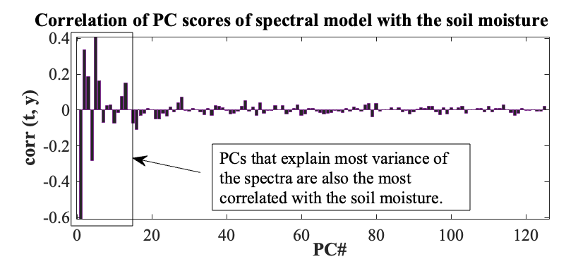
Case I. Hyperspectral soil imagery to calibrate moisture soft-sensors. The dataset presented by Riese & Keller, 2018 [12] contains 450 - 950 nm spectra with a spectral resolution of 4 nm. The modelling goal of Case I is to demonstrate the KF optimization and retrieval model performance with KF-PCR. The PCR is preferably utilized in scenarios in which (a) the variables have a high correlation to the response variable, not justifying the utilization of more complex methods, and (b) the data is high-dimensional. Figure 1 showcases the correlation between PCs in the original space and the response variable.
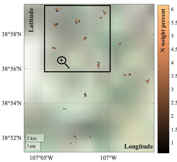
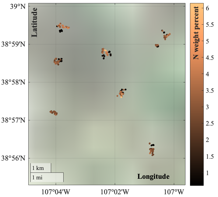
Case II. Hyperspectral vegetation airborne imagery to calibrate plant trait soft sensors. The dataset introduced in Chadwik et al., 2020 [3] was originally modelled with PLS. The goal of the case is to evaluate if KF-PLS with the proposed loss function is competitive compared to other non-linear methods. The trait presented in the results is illustrated in Fig. 2. The mass percentage of Nitrogen in the needle trees has been chosen for showcasing due to its low performance in the linear methods [3].
(a)
(b)
V Results and Discussion
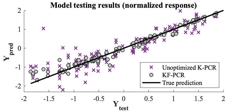
Case I. The first case study showcases a scenario in which the response variable (soil moisture) is highly correlated with the response variable. As seen in Figure 3, the unoptimized K-PCR model has higher residuals for test partition prediction. In the unoptimized version, all kernel parameters have the value ’1’. A combination of kernels is able to minimize the residuals and achieve better precision with only one nonlinear PC.
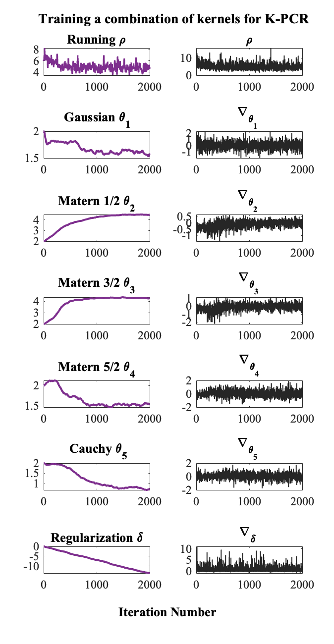
In Figure 4, the learning process for a combination of kernels is presented. Compared to the training process using the traditional KF loss, [8], the training process is less stable, with a larger variation in the loss. Some parameters converge into a steady value, while others have a slight variation around the convergence value. This occurs due to (i) the kernel parameters being correlated to each other or (ii) the kernel not having an important role in the combination of kernels. The mean of the gradient component for the kernel parameters approaching convergence is 0 for all converged parameters.
Case II. KF-PLS emerged as the top performer, followed by GPR. The GPR model, utilizing the Rational Quadratic kernel, had a parameter for each wavelength and took over 3000 seconds to train, while KF-PLS only fitted only two parameters and trained in 107 seconds. KF-PLS and KF-PCR outperformed linear methods due to their ability to capture non-linearity in the dataset. Additionally, they reduced the risk of overfitting, outperforming some of the non-linear methods, by learning fewer parameters and due to the the cross-validative nature of KF. When compared to the original KF loss [9], the updated KF loss brought a +33% performance improvement in the KF-PCR, and a +2% improvement in the KF-PLS results.
| Method | Optimized | |
|---|---|---|
| KF-PLS (modified ) | Matern5/2 | 0.580 |
| KF-PCR | Cauchy | 0.481 |
| PLS (Original article) | Ref. [3] | 0.201 |
| Linear Regression | - | 0.331 |
| Tree | Coarse | 0.290 |
| SVM | Cubic | 0.518 |
| Efficient Linear | Least-Squares | 0.023 |
| Ensemble | Bagged Trees | 0.459 |
| GPR | Rational Quadratic | 0.531 |
| Neural Network | Bilayered | 0.359 |
VI Conclusions
In this paper, we propose a method to optimize the kernel parameters for K-PCR using a modified KF approach. Our results demonstrate an improvement in soil moisture prediction from hyperspectral airborne data by utilizing a combination of kernels. We also tested this new approach with KF-PLS in a case study focused on estimating nitrogen weight content in plants from airborne spectra, where the spectra and responses were not highly collinear. The results consistently outperformed other linear and non-linear methods, indicating that our approach is effective for optimizing KF-PLS as well.
The method shows great potential for various hyperspectral data analysis. Apart from the illustrated environmental retrieval models on soil moisture and plant traits, the models can be extended to water quality retrieval models. Biogeophysical quantity maps can be generated from the models with more accuracy, as the proposed kernel-based models do not overfit the training data. The optimized kernel methods also have the potential of replacing traditional PLS in hyperspectral pansharpening models.
This study has limitations related to the selection of training data for model calibration. Larger training datasets lead to increased kernel matrices and longer training times. Future work could explore sample selection strategies for optimal kernel construction following parameter optimization.
VII Acknowledgements
Funding from Research Council of Finland for Centre of Excellence of Inverse Modelling and Imaging, project number 353095, is acknowledged. The Research Council of Finland, through the Flagship of Advanced Mathematics for Sensing, Imaging and Modelling, decision number 359183, is also acknowledged. The research effort by JS and OL was carried out at the Jet Propulsion Laboratory, California Institute of Technology, under a contract with the National Aeronautics and Space Administration (80NM0018D0004).
References
- [1] Clémence Goyens, Héloïse Lavigne, Antoine Dille, and Han Vervaeren, “Using hyperspectral remote sensing to monitor water quality in drinking water reservoirs,” Remote Sensing, vol. 14, no. 21, pp. 5607, 2022.
- [2] Marie Weiss, Frédéric Jacob, and Grgory Duveiller, “Remote sensing for agricultural applications: A meta-review,” Remote sensing of environment, vol. 236, pp. 111402, 2020.
- [3] K Dana Chadwick, Philip G Brodrick, Kathleen Grant, Tristan Goulden, Amanda Henderson, Nicola Falco, Haruko Wainwright, Kenneth H Williams, Markus Bill, Ian Breckheimer, et al., “Integrating airborne remote sensing and field campaigns for ecology and earth system science,” Methods in Ecology and Evolution, vol. 11, no. 11, pp. 1492–1508, 2020.
- [4] Alison Beamish, Martha K Raynolds, Howard Epstein, Gerald V Frost, Matthew J Macander, Helena Bergstedt, Annett Bartsch, Stefan Kruse, Victoria Miles, Cemal Melih Tanis, et al., “Recent trends and remaining challenges for optical remote sensing of arctic tundra vegetation: A review and outlook,” Remote Sensing of Environment, vol. 246, pp. 111872, 2020.
- [5] Akin Ozdemir and Kemal Polat, “Deep learning applications for hyperspectral imaging: a systematic review,” Journal of the Institute of Electronics and Computer, vol. 2, no. 1, pp. 39–56, 2020.
- [6] T ZHENG, N QUEALLY, KD CHADWICK, J CRYER, P REIM, P TOWNSEND, E MARSH, M BERG, Z BREUER, N BURKARD, et al., “Shift: Reflectance measurements for dried and ground leaf materials,” ORNL DAAC, 2023.
- [7] Gamze Guven and Hatice Samkar, “Examination of dimension reduction performances of plsr and pcr techniques in data with multicollinearity,” Iranian Journal of Science and Technology, Transactions A: Science, vol. 43, pp. 969–978, 2019.
- [8] Zina-Sabrina Duma, Jouni Susiluoto, Otto Lamminpää, Tuomas Sihvonen, Satu-Pia Reinikainen, and Heikki Haario, “Kf-pls: Optimizing kernel partial least-squares (k-pls) with kernel flows,” Chemometrics and Intelligent Laboratory Systems, vol. 254, pp. 105238, 2024.
- [9] Houman Owhadi and Gene Ryan Yoo, “Kernel flows: From learning kernels from data into the abyss,” Journal of Computational Physics, vol. 389, pp. 22–47, 2019.
- [10] Otto M Lamminpää, Jouni I Susiluoto, Jonathan M Hobbs, James L McDuffie, Amy J Braverman, and Houman Owhadi, “Forward model emulator for atmospheric radiative transfer using gaussian processes and cross validation,” Atmospheric Measurement Techniques Discussions, vol. 2024, pp. 1–32, 2024.
- [11] Roman Rosipal and Leonard J Trejo, “Kernel partial least squares regression in reproducing kernel hilbert space,” Journal of machine learning research, vol. 2, no. Dec, pp. 97–123, 2001.
- [12] Felix M. Riese and Sina Keller, “Hyperspectral benchmark dataset on soil moisture,” , 2018.