Horticultural Temporal Fruit Monitoring via
3D Instance Segmentation and Re-Identification using Point Clouds

Abstract

Robotic fruit monitoring is a key step toward automated agricultural production systems. Robots can significantly enhance plant and temporal fruit monitoring by providing precise, high-throughput assessments that overcome the limitations of traditional manual methods. Fruit monitoring is a challenging task due to the significant variation in size, shape, orientation, and occlusion of fruits. Also, fruits may be harvested or newly grown between recording sessions. Most methods are 2D image-based and they lack the 3D structure, depth, and spatial information, which represent key aspects of fruit monitoring. 3D colored point clouds, instead, can offer this information but they introduce challenges such as their sparsity and irregularity. In this paper, we present a novel approach for temporal fruit monitoring that addresses point clouds collected in a greenhouse over time. Our method segments fruits using a learning-based instance segmentation approach directly on the point cloud. Each segmented fruit is processed by a 3D sparse convolutional neural network to extract descriptors, which are used in an attention-based matching network to associate fruits with their instances from previous data collections. Experimental results on a real dataset of strawberries demonstrate that our approach outperforms other methods for fruits re-identification over time, allowing for precise temporal fruit monitoring in real and complex scenarios.

I Introduction

The challenge of meeting a growing demand for food requires advances in agricultural practices, with a focus on efficiency and sustainability. Autonomous robots offer new possibilities to automate labor-intensive tasks such as crop monitoring and management. Such systems have the potential to enhance agricultural production systems, and can enable continuous and large-scale monitoring [8, 38, 33]. In particular, these technologies support phenotyping, the process of evaluating plant characteristics by providing precise, high-throughput assessments and surpass the limitations of traditional manual methods [9, 40]. This shift towards automated phenotyping represents a critical step forward in optimizing crop selection and improving crop yield. Temporal matching, or fruit re-identification, on top of accurate instance segmentation, allows for tracking the development of single fruits over time, enabling the analysis of growth patterns and the estimation of maturation rates.

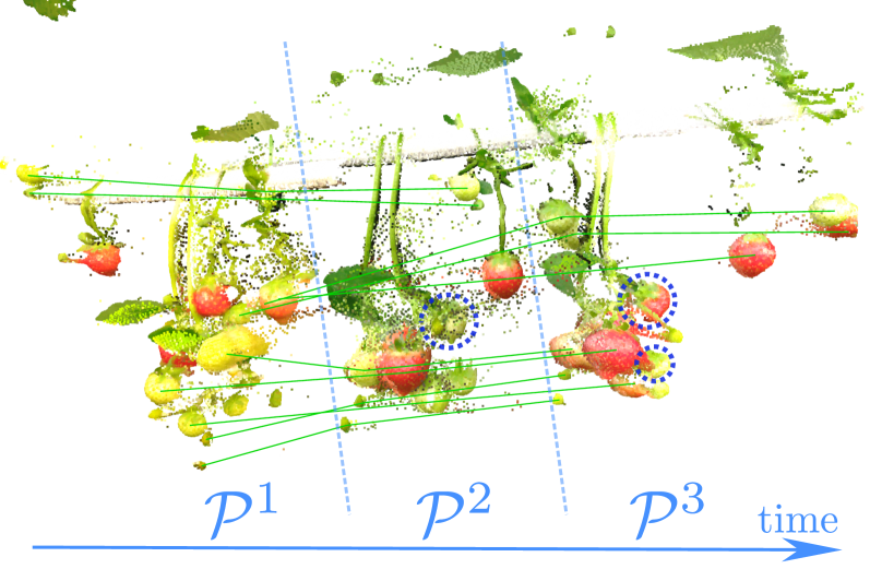
Figure 1: Fruit re-identification on three point clouds acquired at three different points in time. Fruit instances are first segmented using an instance segmentation method, then they are temporally matched with fruit instances of a previous data collection (e.g., matching fruits in $\mathcal{P}^{t}$ with fruits in $\mathcal{P}^{t-1}$). Green lines indicate matching between fruits, while fruits inscribed in a circle do not have a matching fruit in the previous data collection.

In this paper, we aim to track fruits in a greenhouse using colored point clouds acquired by a robot equipped with a high-resolution LiDAR scanner. The goal is to identify, segment, and temporally match individual fruits at different points in time within the 3D space. 2D image-based approaches [30, 10, 13, 11, 19] lack the 3D structure, depth, and spatial information offered by point clouds. Conversely, point clouds lack a regular grid structure, making it difficult to apply traditional image processing techniques. The challenge is to process this sparse and irregular data to detect and associate individual fruits, which may vary in size, shape, orientation, and occlusion levels and may be harvested or newly grown.

Once fruit instances have been segmented, the re-identification task involves recognizing and matching the same fruit instances across different point clouds captured at different points in time or from different viewpoints. Similar to loop closures in SLAM [35] and visual place recognition [37] systems, this task is usually performed assuming unique landmarks. In the context of fruit re-identification, there are no unique traits that make fruits easily distinguishable. As depicted in Fig. 1, fruits can be very similar, tightly packed, and their pose can change significantly over time, causing trivial solutions based on relative position to fail.

The main contribution of this paper is a novel method for accurately performing fruit instance segmentation and re-identification on point clouds captured by an agricultural robot at different points in time, based on a learned descriptor encoder and an attentive matcher. We exploit dense high-precision point clouds recorded with a high precision Faro laser scanner. While these sensors are not commonly employed in robotic applications, their capability to scan detailed environments has recently garnered attention, leading to their integration into robotic systems [33]. We segment fruits using a learning-based instance segmentation, which infers fruit instances directly from the point cloud. Each fruit is then processed by a 3D sparse convolutional neural network to obtain a per instance descriptor. Then, we match each fruit with its corresponding instance from a previous data collection by using their descriptors and an attention-based matching neural network. To handle the possibility of a no-match scenario, where a query fruit is identified as a new instance, we represent it using a specific descriptor. We then predict a probability distribution over the candidate fruits from a previous data collection, including the no-match option. Each query fruit is subsequently matched with the previous instance that has the highest predicted probability, using a greedy assignment to determine associations.

In sum, we make two key claims: (i) our approach is able to identify fruits in point clouds using an instance segmentation method; (ii) it outperforms baseline approaches on the re-identification task using real-world data collected in a greenhouse. These claims are backed up by the paper and our experimental evaluation. By harnessing 3D data and sparse convolution networks, our method significantly enhances the effectiveness and scalability of fruit segmentation and tracking, outperforming baseline approaches and offering new capabilities in automated crop monitoring. The implementation of our method is available at https://github.com/PRBonn/IRIS3D.

II Related Work

General instance segmentation, the task of segmenting individual objects within a scene, has been extensively studied in the context of 2D images. In this domain, the Mask R-CNN [17] architecture has emerged as one of the most popular methods. It is a deep learning architecture that extends the object detection process by adding a parallel branch that predicts segmentation masks, allowing precise localization of object boundaries. It has been applied to several fruit instance segmentation tasks on images [30, 10, 13, 11]. Differently from standard Mask R-CNN, Weikuan et al. [19] implement an anchor-free inference pipeline intended to make the model more stable and easily applied to other green fruits without hyper-parameters tuning.

However, the task of instance segmentation becomes significantly more challenging when applied to 3D data like point clouds obtained using RGB-D cameras or LiDAR sensors. Most neural network-based approaches to instance segmentation on point clouds [6, 42] voxelize the 3D point cloud to preserve topological relations and use sparse convolutions [14] to reduce the memory consumption. Despite these advancements, few works have specifically addressed 3D fruit instance segmentation. Kang et al. [20] fuse point clouds and images to perform fruit localization using a single-stage instance segmentation network. Magistri et al. [26] exploit shape completion and differentiable rendering techniques to estimate the 3D shape of a target fruit together with its pose even under strong occlusions from a single RGB-D image.

Image-based phenotyping for the automated monitoring of plants has become increasingly important in numerous agricultural settings. Computer vision, aided by deep learning techniques, has been applied to different phenotyping-oriented agricultural contexts [21, 29, 15, 34, 3, 12].

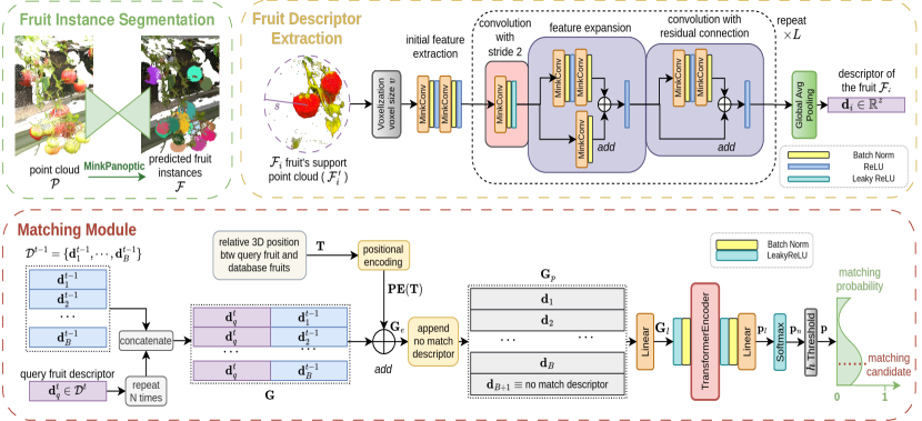
Figure 2: Top: the fruit descriptor extraction module processes a fruit’s support point cloud, $\mathcal{F}^{\prime}_{i}$, and computes the fruit descriptor, $\mathbf{d}_{i}$. It initially voxelizes the input point cloud, then, a MinkowskiNet [6] encoder processes the voxelized point cloud by leveraging sparse 3D convolutions. A final global average pooling aggregates the features of all the voxels to compute the descriptor. Below: the fruit descriptors matching module matches a query descriptor with a set of descriptors of fruits that belong to a different point in time.

Although image-based phenotyping has garnered considerable attention, there are relatively few studies that proposed methods for plant phenotyping using 3D data. Hao et al. [16] analyze and evaluate the degree of wilting of cotton varieties in point clouds. Boogaard et al. [4] investigate the problem of internode length measurements in cucumbers by comparing estimates from 3D point clouds with estimates from images.

A key factor contributing to the gap between 2D and 3D analysis lies in sensor limitations. For instance, conventional sensors used on robots, such as 3D LiDARs and RGB-D cameras, typically offer a 3D spatial resolution that is insufficiently detailed for agricultural environments. One potential solution is to utilize high-precision laser scanners to generate dense, colored, and highly accurate point clouds. Such data has also been used in the past. For example, Rodriguez-Sanchez et al. [32] showcase the use of a ground robot to automate terrestrial laser scanner (TLS) data acquisition in a breeding field.

There is also a limited number of studies focusing on temporal fruit matching, i.e., the problem of finding fruit correspondences over time. Chebrolu et al. [5] exploit a skeletal structure to compute correspondences between the same plant over two weeks to estimate leaf growth parameters. We, instead, use more realistic data from commercial greenhouses. Riccardi et al. [31] propose a histogram descriptor that utilizes Euclidean distance measurements between neighboring fruits. For a given target fruit, their method divides the surrounding 3D space into angular sectors and counts the number of fruits within each sector. Lobefaro et al. [25] investigate the problem of 4D data associations estimation in growing pepper plants in a green house by combining 3D RGB-D SLAM for building local plant models and visual place recognition to create the correspondences across time. The same authors, in a following work et al. [24], employ deep-learning-based feature descriptors and geometric information to obtain matches between 3D points and track the plant traits’ evolution over time.

We rely on MinkowskiNet [6] for our instance segmentation method. Based on such a segmentation, we can address different downstream tasks, like plant and fruit phenotyping. We use a learned descriptor, based on 3D sparse convolution, to automatically learn and extract relevant features from raw data through training, allowing it to adapt to complex patterns and variations in the data. Also, our learned descriptor can adapt to new and unseen data without requiring explicit re-engineering of feature extraction methods. We perform descriptor matching leveraging an attention-based network that predicts a probability distribution over the pool of candidate matchings, considering also the no-match case.

III Our Approach

We aim to track fruits in a greenhouse using data acquired by a robot. Thus, we present a novel method for accurately performing fruit instance segmentation and re-identification on point clouds captured at different points in time.

III-A Fruit Instance Segmentation Module

Consider a colored point cloud $\mathcal{P}$ in which each point has six properties: the 3D position and the RGB color. We want to segment $\mathcal{P}$ into a set $\mathcal{F}=~{}\{{\mathcal{F}_{i}}\}^{K}_{i=1}$ of $~{}K$ fruit instances. Each $\mathcal{F}_{i}\subseteq\mathcal{P}$ can be also described by the pair $(\mathbf{c}_{i},r_{i})$, where $\mathbf{c}_{i}\in\mathbb{R}^{3}$ is the center of the fruit, given by:

$$\mathbf{c}_{i}=\frac{1}{|\mathcal{F}_{i}|}\sum_{\mathbf{p}_{j}\in\mathcal{F}_{i}}{\mathbf{p}_{j}}$$ (1)

and $r_{i}$ is the radius of the smallest sphere, centered at $\mathbf{c}_{i}$, containing all the fruit’s points. Note that $\mathbf{c}_{i}$ does not necessarily correspond to a point of the point cloud.

We use MinkPanoptic [27], a learning-based instance segmentation method, to obtain the fruit instances in a point cloud. MinkPanoptic first infers the semantic segmentation, dividing points into fruit and background classes.

Let $\mathcal{P}_{f}\subseteq\mathcal{P}$ be the subset of $\mathcal{P}$ that was labeled as fruit. Then, for each point in $\mathcal{P}_{f}$, the method predicts a 3D vector representing the point’s offset from the center of the fruit instance it belongs to. We add the predicted offsets to $\mathcal{P}_{f}$ to get the point cloud $P_{o}$. We determine fruit instances $\mathcal{F}$ by clustering $~{}P_{o}$ using the mean shift [7] algorithm. Clustering-based methods generally obtain better performance than end-to-end instance segmentation approaches [41].

III-B Fruit Descriptor Extraction Module

The fruit descriptor extraction module processes fruit instances obtained with the instance segmentation method described in Sec. III-A and computes their descriptors. Given a fruit $\mathcal{F}_{i}$ and its center $\mathbf{c}_{i}$, we define with $\mathcal{S}_{i}\subseteq\mathcal{P}$ the support of $\mathcal{F}_{i}$ with fixed radius $s$:

$$\mathcal{S}_{i}=\{\mathbf{p}\in\mathcal{P}\mid\|\mathbf{p}-\mathbf{c}_{i}\|_{2}\leq s\}.$$ (2)

The usage of $\mathcal{S}_{i}$ instead of $\mathcal{F}_{i}$ enables the descriptor extraction to account also for the surrounding of the fruit $\mathcal{F}_{i}$. We want the descriptor to be as discriminative as possible between different fruits, but as similar as possible for the point clouds of the same fruit taken at different points in time. Also, the descriptor should be robust for rotation, shape, and color variation. Fruits often change their orientation during growth, but also their shape changes substantially. The color changes both due to the growth of the fruit and due to the greenhouse’s internal light change (position of the sensor, outside weather, humidity, artificial light, etc.).

On top of Fig. 2, the fruit descriptor extraction module architecture is depicted. First of all, the fruit support point cloud $\mathcal{S}_{i}$ is voxelized using a fixed voxel size $v$. Then, a MinkowskiNet encoder processes the voxelized point cloud by leveraging sparse 3D convolutions, capturing multi-scale features through a deep hierarchical structure.

The encoder is composed of multiple stages that progressively downsample the input spatial dimensions while increasing the number of feature channels. It begins with two sparse 3D convolutional layers, each followed by batch normalization (BN) [18] and a ReLU, responsible for initial feature extraction from the input sparse tensor. Then, $L$ identical blocks sequentially process the sparse tensor.

Each block is comprised of three parts. The first part performs downsampling (via a convolution with a stride of 2), reducing the spatial resolution while expanding the receptive field. The second part comprises a main convolutional path, that applies two sequential 3D sparse convolutions with a $3\times 3$ kernel, BN, and ReLU activation, expanding the feature channels, and a secondary path consisting of a single convolution with $1\times 1$ kernel that matches the dimensions of the input to the output, followed by BN. The third part is very similar to the second one, except that the secondary path consists of a simple residual connection.

After the $L$ identical blocks, we apply a global average pooling, which aggregates features across all the voxels obtaining the fruit’s descriptor $\mathbf{d}_{i}\in\mathbb{R}^{z}$.

By computing the descriptors of all the fruits $\mathcal{F}$, we build a set of descriptors $\mathcal{D}=\{\mathbf{d}_{1},\dots,\mathbf{d}_{|\mathcal{F}|}\}$ where $\mathbf{d}_{i}$ represents the descriptor of fruit $\mathcal{F}_{i}$.

III-C Fruit Descriptors Matching Module

The fruit descriptors matching module operates on sets of descriptors of fruits that belong to different time steps. Let $\mathcal{D}^{t}$ be the set of descriptors of all the fruits segmented at time $t$, i.e., $\mathcal{F}^{t}=\{\mathcal{F}_{1}^{t},\dots,\mathcal{F}_{A}^{t}\}$, and $\mathcal{D}^{t-1}$ the set of descriptors of all the fruits segmented at time ${t-1}$, i.e., $\mathcal{F}^{t-1}=\{\mathcal{F}_{1}^{t-1},\dots,\mathcal{F}_{B}^{t-1}\}$.

We want to match descriptors in $\mathcal{D}^{t}$ with the corresponding descriptors in $\mathcal{D}^{t-1}$. Moreover, we also want to label new or simply not visible fruits descriptors with a no-match label, $\varnothing$. Formally, we want to compute the association vector $\mathbf{y}=[y_{1},\dots,y_{A}]^{\top}$ with $y_{i}\in\{\varnothing,1,\dots,B\}$.

Let $\mathcal{F}_{q}^{t}\in\mathcal{F}^{t}$ be a query fruit point cloud at time $t$ and $\mathbf{d}_{q}^{t}\in\mathcal{D}^{t}$ be its descriptor. To infer $y_{q}$, the matching module computes the probability distribution $p(\mathbf{y}\mid\mathcal{D}^{t},\mathcal{D}^{t-1})$. The matching module processes the descriptor $\mathbf{d}_{q}^{t}$ and the set of descriptors $\mathcal{D}^{t-1}$. It also exploits the relative position $\mathbf{T}\in\mathbb{R}^{B\times 3}$ between the query fruit and the fruits in $\mathcal{F}^{t-1}$.

Fig. 2 below depicts the matching module’s architecture. First, $\mathbf{d}_{q}^{t}$ is concatenated to each descriptor in $\mathcal{D}^{t-1}$, obtaining the matrix $\mathbf{G}\in\mathbb{R}^{B\times 2z}$ To focus the module on the neighbors of the query fruit, we add a fixed positional encoding $\mathbf{PE}$ to $\mathbf{G}$ obtaining $\mathbf{G}_{e}$:

$$\mathbf{G}_{e}=\mathbf{G}+\mathbf{PE}(\mathbf{T}).$$ (3)

We compute $\mathbf{PE}:\mathbb{R}^{3}\mapsto\mathbb{R}^{z}$ as a function of the relative position matrix $\mathbf{T}$ applied to each row as done in Mildenhall et al. [28], i.e., we apply it to each individual coordinate.

To let the matching module account for the no-match case, we artificially create a new row in $\mathbf{G}_{e}$ representing the no-match case. The new element is a descriptor with all zero elements and is appended to $\mathbf{G}_{e}$ as the last row, obtaining the matrix $\mathbf{G}_{p}\in\mathbb{R}^{(B+1)\times 2z}$.

A linear layer, followed by BN and leaky ReLU, maps $\mathbf{G}_{p}$ to $\mathbf{G}_{l}\in\mathbb{R}^{(B+1)\times l}$, and a transformer encoder layer [36], followed by BN and leaky ReLU, processes $\mathbf{G}_{l}$ obtaining $\mathbf{G^{\prime}}_{l}\in\mathbb{R}^{(B+1)\times l}$. A final linear layer maps $\mathbf{G^{\prime}}_{l}$ to the prediction logits vector $\mathbf{p}_{l}\in\mathbb{R}^{B+1}$, which are then normalized into a probability distribution $\mathbf{p}_{n}$ by applying a softmax. To impose the assumption that fruits do not move, between scans, more than $h\in\mathbb{R}$ meter, we mask $\mathbf{p}_{n}$ by setting the probability of fruits whose center is at a distance greater than $h$ to $0$, obtaining $\mathbf{p}$.

The predicted matching fruit’s index $y_{q}$ is given by:

$$y_{q}=\begin{cases}i,&\text{if }i<B+1\\ \varnothing&\text{if }i=B+1\end{cases},~{}\text{with}~{}~{}i=\mathop{\rm argmax}_{i}{(\mathbf{p})}$$ (4)

By predicting $y_{i}$ for each fruit in $\mathcal{F}_{i}^{t}$, we can associate each fruit in $\mathcal{F}_{i}^{t}$ to fruits in $\mathcal{F}_{i}^{t-1}$ with the vector $\mathbf{y}$.

III-D Batch Matching

When matching more than one fruit, we post-process $\mathbf{y}$ using a greedy matching algorithm. Specifically, let $\mathbf{H^{*}}\in~{}\mathbb{R}^{A\times(B+1)}$ be the matrix representing all the probability distributions predicted with the matching module, associating all the fruits in $\mathcal{F}^{t}$ to those in $\mathcal{F}^{t-1}$. The element $\mathbf{H^{*}}_{ij}$ at row $i$ and column $j\leq B$ represents the probability of the fruit $\mathcal{F}_{i}^{t}$ matching with $\mathcal{F}_{j}^{t-1}$. The last column of $\mathbf{H^{*}}$ encodes the no-match probability of each fruit in $\mathcal{F}^{t}$. Also, each row $i$ of $\mathbf{H^{*}}$ corresponds to the vector $\mathbf{p}$ computed for $\mathcal{F}_{i}^{t}$.

We compute the vector of associations $\mathbf{y}$ using a greedy approach, starting by matching the most probable fruits first and removing them from the candidate pool. This process continues until all fruits in $\mathcal{F}^{t}$ have either been matched or labeled as unmatched.

III-E Loss Function

We trained the fruit instance segmentation method following Marcuzzi et al. [27], using a loss function $\mathcal{L}_{\text{ins}}$ composed of two terms:

$$\mathcal{L}_{\text{ins}}=\mathcal{L}_{\text{sem}}+\lambda_{\text{off}}\mathcal{L}_{\text{off}}.$$ (5)

The first term, $\mathcal{L}_{\text{sem}}$, accounts for the fruit semantic segmentation, and is a weighted sum of a cross-entropy loss and a Lovász-Softmax loss [2]:

$$\mathcal{L}_{\text{sem}}=\lambda_{\text{ce}}\mathcal{L}_{\text{ce}}+\lambda_{\text{Lov}}\mathcal{L}_{\text{Lovász}}.$$ (6)

The second term, $\mathcal{L}_{\text{off}}$, measures the discrepancy between the predicted and the ground truth offsets. It is given by:

$$\mathcal{L}_{\text{off}}=\frac{1}{|\mathcal{P}_{f}|}\sum_{j=1}^{|\mathcal{P}_{f}|}{\|\mathbf{o}_{j}-\mathbf{\hat{o}}_{j}\|_{1}},$$ (7)

where $\mathbf{o}_{j}\in\mathbb{R}^{3}$ is the $j$-th predicted offset and $\mathbf{\hat{o}}_{j}\in\mathbb{R}^{3}$ is the corresponding ground truth offset.

We trained our descriptor extraction and re-identification method end-to-end by batch matching with a weighted loss function, $\mathcal{L}_{\text{m}}$, composed of two terms:

$$\mathcal{L}_{\text{m}}=\mathcal{L}_{\text{ce}}+\lambda_{\text{inj}}\mathcal{L}_{\text{inj}}.$$ (8)

The first, $\mathcal{L}_{\text{ce}}$, computes the cross-entropy loss between the ground truth matrix $\mathbf{\hat{H}}$ and the predicted matrix $\mathbf{H^{*}}$:

$$\mathcal{L}_{\text{ce}}=\sum_{i=1}^{A}{\sum_{j=1}^{B+1}{-\mathbf{\hat{H}}_{ij}\log(\mathbf{H^{*}}_{ij})}}.$$ (9)

The second, $\mathcal{L}_{\text{inj}}$, forces the network to learn a bijective function. In other words, the network should map distinct fruits of $\mathcal{F}^{t}$ to distinct fruits of $\mathcal{F}^{t-1}$ and vice versa, avoiding assigning multiple fruits from a particular set to the same fruit in the other set. The $\mathcal{L}_{\text{inj}}$ loss ignores the no-match fruit and it is weighted by $\lambda_{\text{inj}}$ in the final $L_{\text{m}}$ loss computation.

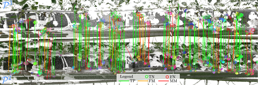
Figure 3: Fruit instance segmentation and re-identification using our method. On the top image, we report the predicted instance segmentation on $\mathcal{P}^{3}$ that we match with the ground truth fruit annotations on $\mathcal{P}^{2}$ depicted below. Instances with the same color reflect ground truth matching. Green line (TP); red line (MM); orange line (FM); green circle (TN); red circle (FN). Best viewed in color.

IV Experimental Evaluation

The main focus of this work is a novel method for fruit monitoring based on fruit instance segmentation and re-identification on point clouds recorded at different moments.

We present our experiments to show the capabilities of our method, focusing on high-precision point clouds of strawberry fruits and plants recorded with a terrestrial laser scanner in a greenhouse. The results of our experiments support our claims: (i) our approach is able to identify fruits in point clouds using an instance segmentation method; (ii) it outperforms baseline approaches on the re-identification task using real-world data collected in a greenhouse.

IV-A Dataset and Metrics

For our experimental evaluation, we extend the dataset by Riccardi et al. [31], which consists of point clouds collected with a high-precision Faro Focus3D-X130 laser scanner in a commercial greenhouse, containing the same row of strawberries at 3 different points in time, each separated by approximately one week. Let’s call them $\mathcal{P}^{1}$, $\mathcal{P}^{2}$, and $\mathcal{P}^{3}$. Each point cloud is associated with a set of ground truth fruit annotations (respectively, $\hat{\mathcal{F}^{1}}$, $\hat{\mathcal{F}^{2}}$, and $\hat{\mathcal{F}^{3}}$, containing 616, 556 and 159 strawberries). Then, fruits in $\hat{\mathcal{F}^{2}}$ are associated to fruit in $\hat{\mathcal{F}^{1}}$. Let $\mathbf{\hat{y}}_{2,1}$ be the ground truth vector of associations. Similarly, fruits in $\hat{\mathcal{F}^{3}}$ are associated to fruits in $\hat{\mathcal{F}^{2}}$ with the vector of associations $\mathbf{\hat{y}}_{3,2}$. In $\mathbf{\hat{y}}_{2,1}$, 56 strawberries from $\hat{\mathcal{F}^{2}}$ are not matched with those in $\hat{\mathcal{F}^{1}}$. In $\mathbf{\hat{y}}_{3,2}$, 5 strawberries from $\hat{\mathcal{F}^{3}}$ are not matched with $\hat{\mathcal{F}^{2}}$.

We trained our instance segmentation and re-identification method on the first two point clouds, $\mathcal{P}^{1}$ and $\mathcal{P}^{2}$. We trained the two tasks separately, and in particular we trained for the re-identification task only using the ground truth fruit detections. We evaluated our method by inferring fruit detections in the third point cloud, $\mathcal{P}^{3}$, and matching them with ground truth annotations in the second point cloud, $\mathcal{P}^{2}$. This approach enables a clear separation between the fruit instance segmentation module and the fruit descriptor extraction and matching modules, allowing for easy integration and replacement of the segmentation component with alternative solutions. This flexibility makes our method highly adaptable and appealing for various applications.

We use panoptic quality (PQ) [23], consisting of segmentation quality (SQ) and recognition quality (RQ), and Intersection over Union (IoU), as metrics to evaluate the instance segmentation capabilities. For analyzing the matching performance we first compute the following metrics: correct matching (CM, correctly matching two strawberries), mismatching (MM, correctly detecting a strawberry as a matching one but relating it with the wrong corresponding strawberry), false matching (FM, incorrectly labeling a no-matching strawberry with a strawberry), true negative (TN, correctly labeling a strawberry with the no-match label), and false negative (FN, incorrectly labeling a matching strawberry with the no-match label).

Based on these, we calculate the following scores:

$$\text{F1}_{p}=\frac{2\text{CM}}{2\text{CM}+\text{MM}+\text{FM}+\text{FN}}$$ (10)

$$\text{F1}_{n}=\frac{2\text{TN}}{2\text{TN}+\text{FM}+\text{FN}}$$ (11)

$$\text{mF1}=\frac{\text{F1}_{p}+\text{F1}_{n}}{2}$$ (12)

TABLE I: Performance of the instance segmentation; values in %.

Class	$\mathbf{RQ}$	$\mathbf{SQ}$	$\mathbf{PQ}$	$\mathbf{IoU}$
Strawberry	52.7	75.5	40.0	63.9

The standard F1 score measures the goodness of the predictive capacity of a model, but it only focuses on the positive class. By averaging the scores in Eq. (12) for positive and negative classes, we get an indicator for both, mF1. In our experiments, we optimized for the mF1 score.

IV-B Implementation Details

In the loss functions, we use as weights $\lambda_{\text{ce}}=2$, $\lambda_{\text{Lov}}=10$, $\lambda_{\text{off}}=10$ and $\lambda_{\text{inj}}=0.08$. We set support radius $s=0.2$ m and voxel size $v=5\cdot 10^{-4}$ m for the fruit descriptor extraction module and maximum matching distance $h=0.05$ m for the fruit descriptor matching module based on empirical evaluation. We use $L=4$ layers using hidden dimensions 8, 8, 16, 16, and 64 (8 is the number of channels produced by the convolution of the initial feature extraction, while the subsequent are each layer’s produced number of channels). We set the matching module transformer layer’s input channel dimension $l$ to 512, feedforward dimension to 1024, and number of heads to 8.

We trained the instance segmentation model with a fixed learning rate of $2\cdot 10^{-2}$, using standard data augmentation techniques such as applying a random yaw rotation, X or Y axis flip, X or Y scale change (with a uniformly random scaling factor in the range [0.95, 1.05]), and point jittering (adding a per-point noise with a normal distribution centered at zero and with variance 0.1 m).

We obtained the instance segmentation of the third point cloud utilizing the trained model and the mean shift clustering algorithm with a bandwidth of 0.01 m.

We trained the descriptor extraction and re-identification model with a fixed learning rate of $3\cdot 10^{-4}$. We augmented the dataset by applying to each input fruit point cloud a random rotation in the range [-30°, 30°] on each of the three axis, a point jittering added per point drawn from a normal distribution centered at zero and with variance $7\cdot 10^{-4}$ m, and a color jittering, modifying each RGB channel with a random gaussian noise drawn from a normal distribution centered at zero and with variance 0.05.

To train the fruit descriptor extraction and re-identification model, we manually divided the training set $\bigl{(}\hat{\mathcal{F}^{1}}$, $\hat{\mathcal{F}^{2}}$, and $\mathbf{\hat{y}}_{2,1}\bigl{)}$ into two non-overlapping sets, grouping corresponding fruits based on their 3D position. We used the first group as training set, containing approximately 80% of the strawberries, and the second as validation set.

IV-C Matching Results

TABLE II: Comparison of the proposed method with baselines at different IoU thresholds and on average on the re-identification task. All values are in %.

Approach	@5% IoU			@10% IoU			@25% IoU			avg
	$\mathbf{F1_{p}}$	$\mathbf{F1_{n}}$	$\mathbf{mF1}$	$\mathbf{F1_{p}}$	$\mathbf{F1_{n}}$	$\mathbf{mF1}$	$\mathbf{F1_{p}}$	$\mathbf{F1_{n}}$	$\mathbf{mF1}$	$\mathbf{F1_{p}}$	$\mathbf{F1_{n}}$	$\mathbf{mF1}$
Nearest Neighbor	76.1	14.3	45.2	73.8	11.5	42.7	58.6	6.5	32.6	69.5	10.8	40.2
Riccardi et al. [31]	56.1	19.6	37.9	52.1	19.7	35.9	43.6	13.9	28.7	50.6	17.7	34.2
Our approach	77.4	41.5	59.5	74.9	37.2	56.1	58.7	27.7	43.2	70.3	35.5	52.9

The first experiment evaluates the performance of our approach. It supports the claim that our method can identify fruits in point clouds using an instance segmentation method and outperforms baseline approaches on the re-identification task using real-world data collected in a greenhouse.

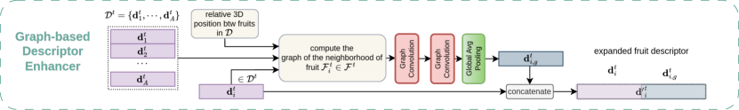
Figure 4: We investigated the significance of neighboring fruits in the descriptor computation. The module builds the graph of the neighborhood of fruit $\mathcal{F}_{i}^{t}$. Two graph convolutions process the graph and a final global average pooling computes the neighborhood descriptor $\mathbf{d}_{i,g}^{t}$, which is concatenated to the original $\mathcal{F}_{i}$ fruit descriptor $\mathbf{d}_{i}^{t}$.

We report in Tab. I the instance segmentation results of MinkPanoptic trained on the first two point clouds, i.e., $\mathcal{P}^{1}$ and $\mathcal{P}^{2}$, and tested on the third point cloud, i.e., $\mathcal{P}^{3}$. The SQ of 75.5% and IoU of 63.9% reflect the model’s capability to accurately delineate the strawberries it detects. It achieves a PQ of 40.0%, indicating moderate overall performance. The RQ of 52.7% suggests that the model’s ability to consistently identify all instances remains an area for improvement.

Then, we compare our re-identification approach with baselines. We match the fruit instance segmentation predicted on $\mathcal{P}^{3}$ at the previous step with the ground fruit annotation of $\mathcal{P}^{2}$. The evaluation is carried out using three different volume IoU thresholds (5%, 10%, and 25%) for associating the predicted instances ID with the ground truth instances ID, and the results are then averaged. Higher IoU thresholds select only the predicted instances that are more similar to the ground truth annotation, introducing many negative instances, while lower IoU thresholds also associate low-quality instance prediction with ground truth annotation, reducing the number of negatives. Each ground truth instance is assigned the ID of the predicted fruit instance with the highest IoU, provided that it exceeds the considered threshold. All not matching predicted fruit instances are assigned a new ID, and thus labeled as negatives.

We consider as baseline methods a nearest neighbor approach fine-tuned with Optuna [1] as well as Riccardi et al. [31]. The first is purely based on the relative position between the sets of fruits and matches them by linking a fruit $\mathcal{F}_{i}^{t}\in\mathcal{F}^{t}$ with the fruit $\mathcal{F}_{*,NN}^{t-1}\in\mathcal{F}^{t-1}$ having the minimum Euclidean distance from $\mathcal{F}_{i}^{t}$. Formally:

$$\mathcal{F}_{*,NN}^{t-1}=\mathop{\rm argmin}_{j}\|\mathbf{c}_{*}^{t}-\mathbf{c}_{j}^{t-1}\|_{2},$$ (13)

where $\mathbf{c}_{i}^{t},\mathbf{c}_{j}^{t-1}$ are the center of the strawberries $\mathcal{F}_{i}^{t},\mathcal{F}_{j}^{t-1}$. This method can match fruits but cannot detect the no-match case. For this reason, we used Optuna, an open-source optimization framework, to find the optimal threshold $\epsilon\in\mathbb{R}$ for which two fruits at a distance larger than $\epsilon$ should be considered unmatchable. A fruit with no matchable counterpart is then considered unmatched. In our experiment, we maximized for the mF1 score in the training set and found the optimal value $\epsilon^{*}=0.033\,m$. Riccardi et al. [31] proposed a histogram descriptor based on the Euclidean distance between neighbor fruits. Considering a target fruit, they divide the 3D space around it into angular sectors and count how many fruits fall in each sector. In our experiments, we use the parameter setting suggested in the original implementation.

The results are reported in Tab. II. Our method consistently achieves the highest performance across all metrics in the test set, with an average mF1 score of 52.9%, outperforming the second-best method by 12.7%. The nearest neighbor approach generally surpasses Riccardi et al. in $\text{F1}_{p}$ score. Conversely, Riccardi et al. obtains generally better $\text{F1}_{n}$ with respect to the nearest neighbor method.

Fig. 3 shows the test result of our method. Despite the detector faults, it outperforms baselines in this demanding scenario.

IV-D Ablation Study

We conducted experiments to evaluate the impact of various design choices on our method. For each experiment, we performed a 5-fold cross-validation on the training set $\bigl{(}\hat{\mathcal{F}^{1}}$, $\hat{\mathcal{F}^{2}}$, and $\mathbf{\hat{y}}_{2,1}\bigl{)}$ that we manually divided into five subsets based on the 3D position of strawberries. We tested different configurations of our fruit descriptor extraction and re-identification method, repeating each experiment four times with different seeds and averaging the results to minimize the effect of randomness. The results are in Fig. 5.

Initially, we validated our re-identification method using a fixed matching module configuration, examining various hidden dimensions for the fruit encoder. The configuration with hidden dimensions [8, 8, 16, 16, 64] achieved the highest performance, with the best mF1 score of 61.2%, $\text{F1}_{p}$ of 75.5% and $\text{F1}_{n}$ of 47.0%.

Next, we examined the effect of augmenting the transformer encoder layer’s feedforward dimension from 512 to 1024 to determine if a more complex network could obtain better performance. The matcher with hidden dimensions [8, 16, 32, 32, 32] yielded the best in subset mF1 score of 60.2%, although this was still lower than the previous results.

Finally, we explored the significance of incorporating neighboring fruits in the descriptor computation. We modified the descriptor extraction module to include a graph-based neural network that computes the neighboring fruits descriptor, and concatenates this to the original fruit descriptor. The architecture is depicted in Fig. 4. We tested 2 graph convolutional operators: GCNConv [22] and EdgeConv [39]. We kept fixed descriptor extractor hidden dimensions [8, 8, 16, 16, 64] and tried different matcher feedforward dimensions, i.e., 512 and 1024. The method employing the convolution operator GCNConv, with feedforward dimension 512, obtained the best in subset mF1 score of 61.0%, (0.2% less than the original, graph-free method) and the overall best $\text{F1}_{n}$ of 47.1%. Conversely, EdgeConv with feedforward dimension 1024 obtains the overall best $\text{F1}_{p}$ of 76.9%.

In summary, our evaluation suggests that our graph-free method composed of an encoder with hidden dimensions [8, 8, 16, 16, 64] and a matching module with a transformer’s feedforward dimension 512 demonstrated to be the best performing in the cross-validation and the test set evaluation.

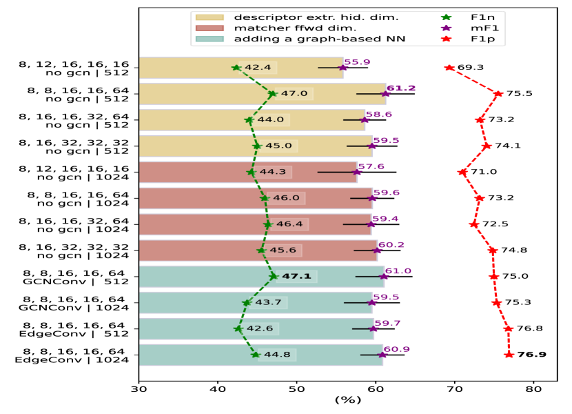
Figure 5: Ablation study to evaluate the impact of various design choices on our method. All values are in %. The horizontal lines depict the standard deviation of mF1.

V Conclusion

In this paper, we presented a novel approach for fruit monitoring over time based on fruit instance segmentation and re-identification on colored point clouds recorded with a robot in a greenhouse at different points in time. Our method first segments fruits using a learning-based instance segmentation approach, and then each segmented fruit is processed by a 3D sparse convolutional neural network to compute the fruit descriptor. Each fruit is matched with its corresponding instance from a previous data collection by using their descriptors and an attention-based matching neural network. We implemented and evaluated our approach on a real dataset and provided comparisons to other existing techniques. The experiments supported all claims made in this paper and demonstrated that our method achieves superior performance even when trained on ground truth annotations but tested on predicted instance segmentation. This flexibility makes our method highly adaptable to different scenarios, allowing for easy integration and replacement of the segmentation component with alternative solutions.

References

- [1] T. Akiba, S. Sano, T. Yanase, T. Ohta, and M. Koyama. Optuna: A next-generation hyperparameter optimization framework. In Proc. of the Intl. Conf. on Knowledge Discovery and Data Mining, 2019.
- [2] M. Berman, A.R. Triki, and M.B. Blaschko. The Lovász-Softmax Loss: A Tractable Surrogate for the Optimization of the Intersection-Over-Union Measure in Neural Networks. In Proc. of the IEEE/CVF Conf. on Computer Vision and Pattern Recognition (CVPR), 2018.
- [3] P.M. Blok, E.J. van Henten, F.K. van Evert, and G. Kootstra. Image-based size estimation of broccoli heads under varying degrees of occlusion. Biosystems Engineering, 208:213–233, 2021.
- [4] F.P. Boogaard, E.J. van Henten, and G. Kootstra. The added value of 3d point clouds for digital plant phenotyping – a case study on internode length measurements in cucumber. Biosystems Engineering, 234:1–12, 2023.
- [5] N. Chebrolu, F. Magistri, T. Läbe, and C. Stachniss. Registration of Spatio-Temporal Point Clouds of Plants for Phenotyping. PLOS ONE, 16(2), 2021.
- [6] C. Choy, J. Gwak, and S. Savarese. 4D Spatio-Temporal ConvNets: Minkowski Convolutional Neural Networks. In Proc. of the IEEE/CVF Conf. on Computer Vision and Pattern Recognition (CVPR), 2019.
- [7] D. Comaniciu and P. Meer. Mean Shift: A Robust Approach Toward Feature Space Analysis. IEEE Trans. on Pattern Analysis and Machine Intelligence (TPAMI), 24(5):603–619, 2002.
- [8] T. Duckett, S. Pearson, S. Blackmore, B. Grieve, W. Chen, G. Cielniak, J. Cleaversmith, J. Dai, S. Davis, C. Fox, P. From, I. Georgilas, R. Gill, I. Gould, M. Hanheide, A. Hunter, F. Iida, L. Mihalyova, S. Nefti-Meziani, G. Neumann, P. Paoletti, T. Pridmore, D. Ross, M. Smith, M. Stoelen, M. Swainson, S. Wane, P. Wilson, I. Wright, and G. Yang. Agricultural Robotics: The Future of Robotic Agriculture. arXiv preprint, arXiv:1806.06762, 2018.
- [9] F. Fiorani and U. Schurr. Future scenarios for plant phenotyping. Annual review of plant biology, 64:267–291, 2013.
- [10] P. Ganesh, K. Volle, T. Burks, and S. Mehta. Deep orange: Mask R-CNN based orange detection and segmentation. IFAC Proceedings Volumes, 52(30):70–75, 2019.
- [11] J. Gené-Mola, R. Sanz-Cortiella, J.R. Rosell-Polo, J.R. Morros, J. Ruiz-Hidalgo, V. Vilaplana, and E. Gregorio. Fruit detection and 3d location using instance segmentation neural networks and structure-from-motion photogrammetry. Computers and Electronics in Agriculture, 169:105165, 2020.
- [12] A.S. Gomez, E. Aptoula, S. Parsons, and P. Bosilj. Deep regression versus detection for counting in robotic phenotyping. IEEE Robotics and Automation Letters (RA-L), 6(2):2902–2907, 2021.
- [13] S. Gonzalez, C. Arellano, and J.E. Tapia. Deepblueberry: Quantification of blueberries in the wild using instance segmentation. IEEE Access, 7, 2019.
- [14] B. Graham, M. Engelcke, and L. van der Maaten. 3D Semantic Segmentation with Submanifold Sparse Convolutional Networks. In Proc. of the IEEE Conf. on Computer Vision and Pattern Recognition (CVPR), 2018.
- [15] M. Halstead, C. McCool, S. Denman, T. Perez, and C. Fookes. Fruit quantity and ripeness estimation using a robotic vision system. IEEE Robotics and Automation Letters (RA-L), 3(4):2995–3002, 2018.
- [16] H. Hao, S. Wu, Y. Li, W. Wen, J. Fan, Y. Zhang, L. Zhuang, L. Xu, H. Li, X. Guo, and S. Liu. Automatic acquisition, analysis and wilting measurement of cotton 3d phenotype based on point cloud. Biosystems Engineering, 239:173–189, 2024.
- [17] K. He, G. Gkioxari, P. Dollár, and R. Girshick. Mask R-CNN. In Proc. of the IEEE Intl. Conf. on Computer Vision (ICCV), 2017.
- [18] S. Ioffe and C. Szegedy. Batch Normalization: Accelerating Deep Network Training by Reducing Internal Covariate Shift. In Proc. of the Intl. Conf. on Machine Learning (ICML), 2015.
- [19] W. Jia, Z. Zhang, W. Shao, S. Hou, Z. Ji, G. Liu, and X. Yin. Foveamask: A fast and accurate deep learning model for green fruit instance segmentation. Computers and Electronics in Agriculture, 191:106488, 2021.
- [20] H. Kang, X. Wang, and C. Chen. Accurate fruit localisation using high resolution lidar-camera fusion and instance segmentation. Computers and Electronics in Agriculture, 203:107450, 2022.
- [21] J. Kierdorf, I. Weber, A. Kicherer, L. Zabawa, L. Drees, and R. Roscher. Behind the leaves: Estimation of occluded grapevine berries with conditional generative adversarial networks. Frontiers in Artificial Intelligence, 5, 2022.
- [22] T.N. Kipf and M. Welling. Semi-supervised classification with graph convolutional networks. In Proc. of the Intl. Conf. on Learning Representations (ICLR), 2017.
- [23] A. Kirillov, K. He, R. Girshick, C. Rother, and P. Dollár. Panoptic Segmentation. In Proc. of the IEEE/CVF Conf. on Computer Vision and Pattern Recognition (CVPR), 2019.
- [24] L. Lobefaro, M. Malladi, T. Guadagnino, and C. Stachniss. Spatio-Temporal Consistent Mapping of Growing Plants for Agricultural Robots in the Wild. In Proc. of the IEEE/RSJ Intl. Conf. on Intelligent Robots and Systems (IROS), 2024.
- [25] L. Lobefaro, M. Malladi, O. Vysotska, T. Guadagnino, and C. Stachniss. Estimating 4D Data Associations Towards Spatial-Temporal Mapping of Growing Plants for Agricultural Robots. In Proc. of the IEEE/RSJ Intl. Conf. on Intelligent Robots and Systems (IROS), 2023.
- [26] F. Magistri, Y. Pan, J. Bartels, J. Behley, C. Stachniss, and C. Lehnert. Improving Robotic Fruit Harvesting Within Cluttered Environments Through 3D Shape Completion. IEEE Robotics and Automation Letters (RA-L), 9(8):7357–7364, 2024.
- [27] R. Marcuzzi, L. Nunes, L. Wiesmann, J. Behley, and C. Stachniss. Mask-Based Panoptic LiDAR Segmentation for Autonomous Driving. IEEE Robotics and Automation Letters (RA-L), 8(2):1141–1148, 2023.
- [28] B. Mildenhall, P. Srinivasan, M. Tancik, J. Barron, R. Ramamoorthi, and R. Ng. NeRF: Representing Scenes as Neural Radiance Fields for View Synthesis. In Proc. of the Europ. Conf. on Computer Vision (ECCV), 2020.
- [29] S. Nuske, S. Achar, T. Bates, S. Narasimhan, and S. Singh. Yield Estimation in Vineyards by Visual Grape Detection. In Proc. of the IEEE/RSJ Intl. Conf. on Intelligent Robots and Systems (IROS), 2011.
- [30] I. Pérez-Borrero, D. Marín-Santos, M.E. Gegúndez-Arias, and E. Cortés-Ancos. A fast and accurate deep learning method for strawberry instance segmentation. Computers and Electronics in Agriculture, 178:105736, 2020.
- [31] A. Riccardi, S. Kelly, E. Marks, F. Magistri, T. Guadagnino, J. Behley, M. Bennewitz, and C. Stachniss. Fruit Tracking Over Time Using High-Precision Point Clouds. In Proc. of the IEEE Intl. Conf. on Robotics & Automation (ICRA), 2023.
- [32] J. Rodriguez-Sanchez, K. Johnsen, and C. Li. A ground mobile robot for autonomous terrestrial laser scanning-based field phenotyping. arXiv preprint arXiv:2404.04404, 2024.
- [33] J. Rodriguez-Sanchez, J.L. Snider, K. Johnsen, and C. Li. Cotton morphological traits tracking through spatiotemporal registration of terrestrial laser scanning time-series data. Frontiers in Plant Science, 15, 2024.
- [34] C. Smitt, M. Halstead, T. Zaenker, M. Bennewitz, and C. McCool. PATHoBot: A robot for glasshouse crop phenotyping and intervention. In Proc. of the IEEE Intl. Conf. on Robotics & Automation (ICRA), 2021.
- [35] C. Stachniss, J. Leonard, and S. Thrun. Springer Handbook of Robotics, 2nd edition, chapter Chapt. 46: Simultaneous Localization and Mapping. Springer Verlag, 2016.
- [36] A. Vaswani, N. Shazeer, N. Parmar, J. Uszkoreit, L. Jones, A.N. Gomez, L. Kaiser, and I. Polosukhin. Attention Is All You Need. In Proc. of the Conf. on Neural Information Processing Systems (NeurIPS), 2017.
- [37] O. Vysotska and C. Stachniss. Effective Visual Place Recognition Using Multi-Sequence Maps. IEEE Robotics and Automation Letters (RA-L), 4(2):1730–1736, 2019.
- [38] A. Walter, R. Finger, R. Huber, and N. Buchmann. Opinion: Smart farming is key to developing sustainable agriculture. Proceedings of the National Academy of Sciences, 114(24):6148–6150, 2017.
- [39] Y. Wang, Y. Sun, Z. Liu, S.E. Sarma, M.M. Bronstein, and J.M. Solomon. Dynamic graph CNN for learning on point clouds. ACM Trans. on Graphics (TOG), 38(5), 2019.
- [40] M. Watt, F. Fiorani, B. Usadel, U. Rascher, O. Muller, and U. Schurr. Phenotyping: New windows into the plant for breeders. Annual review of plant biology, 71(1), 2020.
- [41] B. Xiang, Y. Yue, T. Peters, and K. Schindler. A review of panoptic segmentation for mobile mapping point clouds. ISPRS Journal of Photogrammetry and Remote Sensing (JPRS), 203:373–391, 2023.
- [42] X. Zhu, H. Zhou, T. Wang, F. Hong, W. Li, Y. Ma, H. Li, R. Yang, and D. Lin. Cylindrical and asymmetrical 3d convolution networks for lidar-based perception. IEEE Trans. on Pattern Analysis and Machine Intelligence (TPAMI), 44(10):6807–6822, 2022.