Efficiency of energy-consuming random walkers: Variability in energy helps
Abstract
Energy considerations can significantly affect the behavior of a population of energy-consuming agents with limited energy budgets, for instance, in the movement process of people in a city. We consider a population of interacting agents with an initial energy budget walking on a graph according to an exploration and return (to home) strategy that is based on the current energy of the person. Each move reduces the available energy depending on the flow of movements and the strength of interactions, and the movement ends when an agent returns home with a negative energy. We observe that a uniform distribution of initial energy budgets results in a larger number of visited sites per consumed energy (efficiency) compared to case that all agents have the same initial energy if return to home is relevant from the beginning of the process. The uniform energy distribution also reduces the amount of uncertainties in the total travel times (entropy production) which is more pronounced when the strength of interactions and exploration play the relevant role in the movement process. That is variability in the energies can help to increase the efficiency and reduce the entropy production specially in presence of strong interactions.
I Introduction
Human everyday activities (e.g., commuting between home and workplace, or shopping) are specific kinds of recurrent diffusion process in which agents travel from one place to another and then return to their starting point after following a trajectory with a number of steps of various lengths Gonzalez ; Scafetta2011 ; Barbosa . An exploration and return (ER) strategy is usually used to model such movements in social and ecological systems song-2010 ; Majumdar2010 ; Benichou2011 ; Pappalardo ; wang2022 . This basic principle has been generalized in many studies to better describe for instance the social, economical, and geometrical aspects of these systems gonzalez-2015 ; vazifeh2021 .
In the past few years, the emergence of location tracking devices (e.g., GPS navigator and smart phones), and location-based services (e.g., Foursquare, Yelp checkin and Google places) provides good opportunities to study human mobility patterns at very different spatial and temporal scales gallotti-2012 ; barthelemy-2019 ; bettencourt-2021 ; batty-2021 ; gonzalez-2022 : from mobility of individuals inside a city to mobility and transportation in an entire country Chowel ; Brockmann ; Vespignani ; gonzalez-2023 . As a consequence, important progresses have been made from reconstruction of population density, mobility patterns and flows Phithakkitnukoon ; Kitamura ; Peng , traffic forecasting and urban planning Nagel ; Wang ; Rozenfeld , marketing campaign and prediction of epidemics Fibich ; Pastor-Satorras , to designing of mobile network protocols Chaintreau .
Efficiency of structure and dynamical processes is essential to maintain a sustainable system like a city horner-2002 ; newman-2006 ; dong-2016 ; latora-2018 ; indaco-2019 ; barthelemy-2022 . However, the majority of research on this subject have focused on simulating the statistical characteristics of human mobility, such as displacement and gyration radius. We know that energy, used by human body or vehicle, plays a key role in transportation and other forms of social activities Kolbl ; boyer-2009 ; Wang22 . It has been observed that the average travel times for different transportation modes (e.g. walking, cycling, bus, or car travel) are inversely proportional to the (physiological) energy consumption rates measured for the respective physical activities Kolbl . Interestingly, when daily travel-time distributions of different transport modes are appropriately scaled, they turn out to have a universal functional relationship Kolbl ; kolbl-2021 .
In this work we are going to investigate the effects of energy consumption and limited energy budgets on a measure of efficiency and entropy production in a movement process which is based on the ER strategy. We see how constraints on energy budgets can influence the movements of these interacting and energy consuming agents, for instance resulting in a subdiffusion regime. In particular, we are interested in the efficiency of such a movement process and its relation to a measure of entropy or uncertainty production in such a process indaco-2020 ; indaco-2021 . We study the number of distinct locations visited by a person per the consumed energy. A greater number of demands are expected to be fulfilled during an urban exploration when a larger number of distinct sites are visited. A reasonable definition of efficiency should also take into account the energy consumed by the agent in this process. Additionally, we are interested in the uncertainty in the travel times which is generated by interactions between the agents. Smaller uncertainties in the travel times are expected to result in a better planning and therefore smaller dissipation.
The paper is organized as follows. We start in Sec. II.1 with a definition of the model and the main parameters. In Sec. II.2 we study an effective one-dimensional model and write a master equation in the continuum limit which can easily be generalized to higher dimensions. A naive mean-field approximation to the equation is presented and the results are compared with the exact solutions of the master equation in one dimension. Section II.3 is devoted to the numerical simulations of the model in two dimensions. Concluding remarks are given in Sec. III.
II Results and Discussion
II.1 Model
We consider agents moving on a two-dimensional square lattice of size . The agents (or persons) start the walks at from the origins (or homes) which are distributed according to a reasonable distribution. We use the population growth model introduced in Ref. Li2017 to construct an initial distribution of the population. More precisely, we start from a unit of population at the center of the 2D square lattice. In each step, one site is chosen with a probability proportional to its population and a unit of population is added if site or at least one of its nearest neighbors is populated ( is free parameter, which leads to the highly dense population near the center and leads to the homogeneous density of population all over the city. In the following we work with . The process continues while the whole population is less than . This growth process generates spatially heterogeneous population densities which are qualitatively close to the empirical distributions.
Each person is given an initial energy budget which is consumed in the links of the path taken by the person. We assume that the change in energy is proportional to a measure of the travel time in link , i.e., with a positive coefficient . The latter depends on the flow of movements in that link at time step when the person enters the link USB ; transport-2011 ,
| (1) |
The parameters and represent the strength of interactions, that is how the flows affect the energy cost given the line capacity . The parameter according to the empirical observations USB . The line capacity associated to the link is given by
| (2) |
where, representing the population density. The case with represents a uniform line capacity all over the city, while represents the case in which the line capacity is proportional to the local population density . In the following, we set , i.e., equal to the average population of the end nodes of link .
At the initial population is given by the population distribution generated by the growth model. The initial energies are sampled either from a delta distribution where all persons have the same energy budget or from a uniform distribution with a maximal variability in energy () but the same average energy . The Kronecker delta function for , otherwise it is zero. At each time step of size , each person with current position and energy budget tries to change its position. With probability
| (3) |
the next position is chosen with equal probability from the set of nearest neighbors of . Here, the positive parameter controls the probability of exploration depending on the available energy . If the agent has enough energy, i.e., , then a large leads to a large exploration probability .
With complementary probability , the person goes to the nearest neighbor which is closer to its home . In words, for positive , the moves resemble a simple random walk (exploration is dominated) if the available energy is larger than the energy scale . On the other hand, the moves are mostly directed towards the origin (return is dominated) when the available energy is smaller than . After any move the energy reduces by as described above. In numerical simulations, we shall end the movement if the person returns home with a negative energy. Moreover, the travel time is measured with the number of travels ; the waiting time which is associated to link at time step just affects the dynamics by decreasing the available energy. Note that for negative , the probability of returning to the origin would be significantly larger than the exploration at the initial stages of the process. In the following, however, we shall consider the more realistic case of .
II.2 An effective model
In this section we consider a single person walking on a one-dimensional chain. The effects of interaction with the others can be modeled by the way that energy is degraded. Let be the probability of being at position and with energy at time . Take and as the probabilities of moving to the right and left directions, respectively. The master equation governing reads as follows,
| (4) |
where, assuming a constant line capacity , the changes in energy are
| (5) | |||
| (6) |
depending on the right and left currents
| (7) | |||
| (8) |
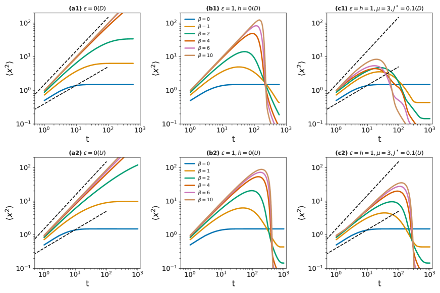
The above discrete equations (with ) are solved numerically to obtain the mean of squared displacement , where denotes averaging with respect to . A particle of average energy is released at time from the center of a chain of length . The mean of squared displacement is reported in Figs. (1) and (2) vs time step and the average energy . In the following, we may omit the time dependence of the average quantities, for instance using for . Note that here we are solving Eq. 4 numerically for the probability distribution starting from an initial condition . We observe that is initially proportional to (normal diffusion) or (subdiffusion) for very large or small , respectively. That is for not very large with . The average number of distinct visited sites in this one-dimensional problem can be estimated as . Then, from Fig. 1 (panels (c1),(c2)) and Fig. 2 (panels (b1),(b2)), we observe that this number is significantly larger in presence of interactions () when the initial energies are distributed uniformly. Later, in Sec. II.3 we will compare the number of distinct visited sites with the consumed energy to have a better measure of efficiency in these processes.
II.2.1 The continuum limit
Here we write the master equation in the continuum limit and present a mean-field solution to the equations. It would be then straightforward to generalize the resulted differential equation to higher dimensions. In the continuum limit , the main equation for the probability density of position and energy of the walker at time can be written as follows
| (9) |
where we defined
| (10) | ||||
| (11) | ||||
| (12) |
where represents the diffusion coefficient, defines drift (external force), and is the rate of energy consumption. The diffusion coefficient represents the stochastic and unbiased part of the motion whereas the drift function quantifies the effect of biases in the process. In general, these functions could depend on the current position and energy of the particle.
Here only terms of order are taken; in the following we assume that and and we set . Moreover, we assume that the right and left transition probabilities differ in a way that results in appropriate diffusion and drift functions,
| (13) | ||||
| (14) |
where , should be an increasing function of . As before we take
| (15) |
and assume that it only depends on energy but not the position of the particle. The scaling with is chosen to have a well-defined continuum limit for the drift function . The step function for , otherwise it is zero. In this way, the diffusion and drift coefficients are given by
| (16) | ||||
| (17) |
Note that in the continuum limit , with
| (18) | ||||
| (19) |
The function determines the system dynamics and shows how the energy is dissipated; if interactions are negligible, the rate of dissipation is expected to be a constant, i.e., . On the other hand, in presence of interactions we may have a dissipation rate that depends on . As before, the parameters and control the strength of interactions.
Now from the master equation we can see how the averages and change with time:
| (20) |
and
| (21) |
We assumed in derivation that and vanish for . In addition, we assume that vanishes for . Recall that
| (22) | ||||
| (23) |
II.2.2 A naive mean-field approximation
We are going to approximate the average of products with the product of averages in equations 20 and 21. Note also that and . Then we get
| (24) | ||||
| (25) | ||||
| (26) | ||||
| (27) |
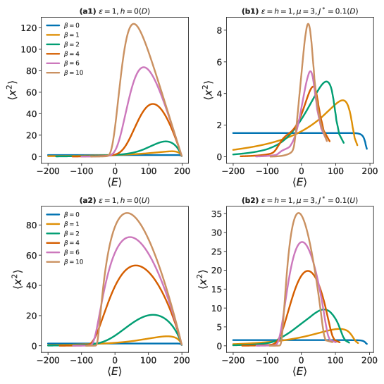
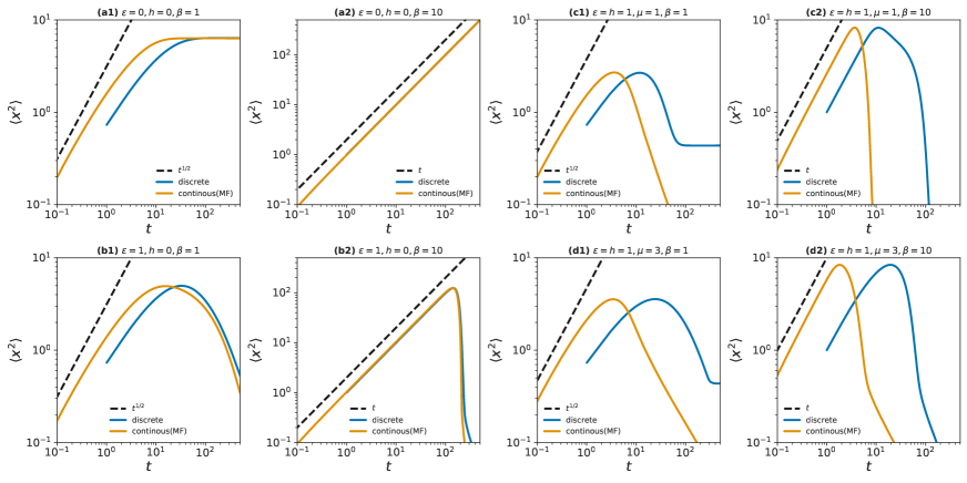
We may also replace . In Fig. (3), we compare the above mean-field approximation with the exact results of the discrete model. Here, the initial energy distribution in the discrete model is concentrated at (delta distribution) as the initial average energy of the particle in the mean-field approximation. We observe that the qualitative behavior of the discrete model is captured by the naive mean-field approximation of the continuum model for different parameter values. The approximation works well especially for small and large .
Note that for small times , where the average energy is still positive, we have for , respectively. Therefore, the second term with negative sign in is more important when is small; for large it is a product of two small quantities and . Thus, we observe a subdiffusion for , whereas for a normal diffusion is observed for small times where the first term dominates. Nevertheless, the average energy decreases faster for larger than for smaller . This for instance can be seen when . In the absence of interactions, the average energy is given by
| (28) |
with initial value at . The time needed to reach average energy zero is
| (29) |
which is a decreasing function of . The relevant time scales in the mean-field equations are
| (30) | ||||
| (31) |
besides, the microscopic time , which is determined by the microscopic length . Recall that we set . In the absence of dissipation, energy is fixed and gives the time we need to reach the stationary state, which is finite as long as . On the other hand, for nonzero the time scale is the time we need to see the effects of dissipation in the energy. Note that dissipation results in a spectrum of time scales for different energies and interactions introduce a range of effective for different times.
Finally, we can say something about the scaling of to have an extended solution to the equations. In the stationary state, or for the maximum range , we get
| (32) | ||||
| (33) |
or
| (34) |
where is stationary energy or the average energy at the maximum range. Assuming that is on order of , the above relation says that to have an extended state we need , where is the linear size of system.
II.3 Numerical simulations
In this section we report the results of numerical simulations of the model described in Sec. II.1 on a two-dimensional square lattice of size . To simplify the picture, in the following we set (i.e., energy is dissipated) and fix the parameter , which is in the range of empirical values USB . The results are reported for two cases of but we mainly focus on case where the link capacities change with the local population (see Eq. 2). The results vary more smoothly with the strength of interactions and are less sensitive to the size and population of the system for compared to the case of uniform line capacity with . We set the initial average energy , to have enough energy for exploring the system by a simple Brownian motion.
Let us begin with the mean energy and the mean-squared-displacement (MSD) of agents, which are defined in terms of an average over the population
| (35) |
| (36) |
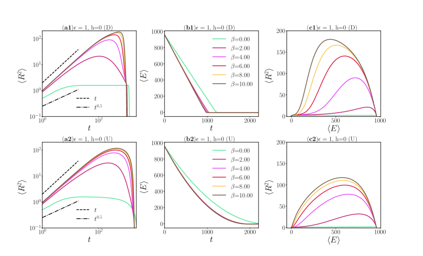
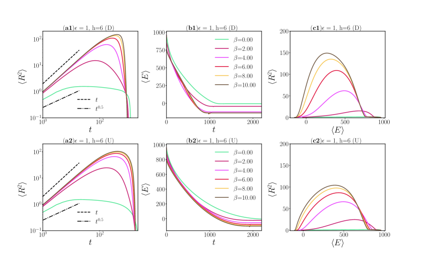
Here denotes averaging over independent realizations of the movement process. Figures (4) and (5) show the MSD and versus time from simulations for a range of values of the control parameters and (with ). Note that for the MSD grows linearly with time at the beginning where pure exploration dominants for each agents. In this regime the probability is close to unity for any and the agent behaves like a simple random walker. On the other hand, for energy dissipation is independent of the traffic, thus after a time of order , almost all the agents have negative energy. Then, return to the origin dominates and the MSD decreases rapidly to zero for . Figure 4 (b2) also shows that even in the absence of interaction, the average energy displays a nonlinear behavior when the initial energy distribution is uniform. That is because the initial energies are very different in this case and is average of the total energy per person.
In the other side, we have the limit where return to origin is dominated and therefore grows sub-linearly with time. In this case a single trajectory of an agent belongs to the class of continuous-time random walks, where the agent’s motion is interrupted by random waiting times. Mostly such processes are characterized by a scaling form of the mean squared displacement,
| (37) |
with metzler2000 . In our model we found that the scaling exponent . As Figs. 4 and 5 show the average energy reduces more slowly when the initial energy has a uniform distribution. In contrast to the one-dimensional model of Sec. II.2 here the MSD is usually larger for the delta energy distribution than the uniform distribution.
Next, to characterize more precisely the performance of the movement process, we study some reasonable measures of efficiency and entropy (uncertainty or disorder) production in the process. In particular, it would be interesting to find the parameters which result in higher efficiencies and lower entropy productions. The definition of efficiency here is based on the mean number of distinct sites visited by the agents and the consumed energy,
| (38) |
Here is the number of distinct sites visited by agent and the denominator represents the total energy consumed by the agent. As mentioned before, an agent starts its movement by the initial energy and stops when returns home with a negative energy at time step .
The average number of distinct sites visited by a random walker after steps has been well studied in the literature, for instance in Dvor . For a foraging animal, corresponds to the size of the territory covered by the animal. In a search algorithm, this quantity corresponds to the number of configurations in the solution space that have been explored. The number of distinct locations visited by a person with a given amount of energy could be a good measure of efficiency of the process; for instance, visiting a larger number of distinct locations enhances the chance of satisfying a larger number of demands.
To see how much the movement process increases disorder in the system we measure the amount of uncertainty in the return times of the agents. Consider a specific realization of the initial population distribution and the initial energy distribution . We simulate the stochastic process of movement for times to find an estimation of the probability distribution of the return times . The entropy production of the process is then defined as:
| (39) |
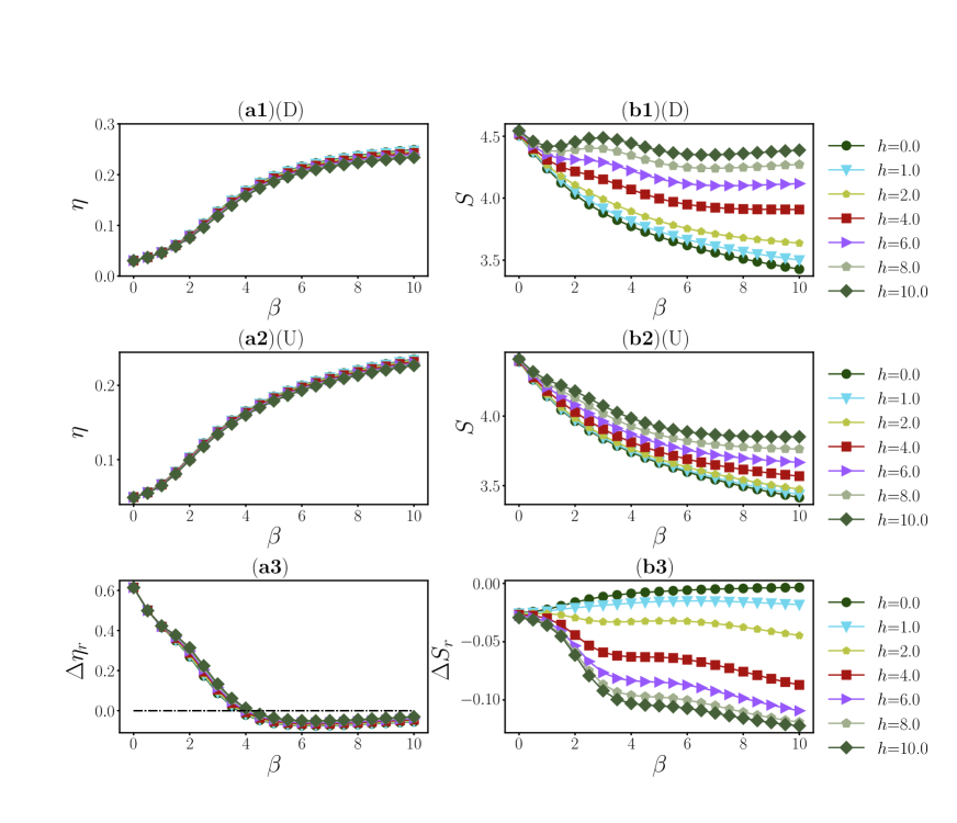
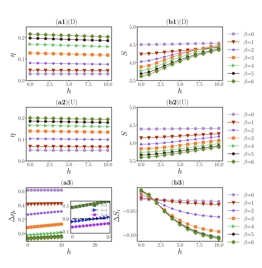
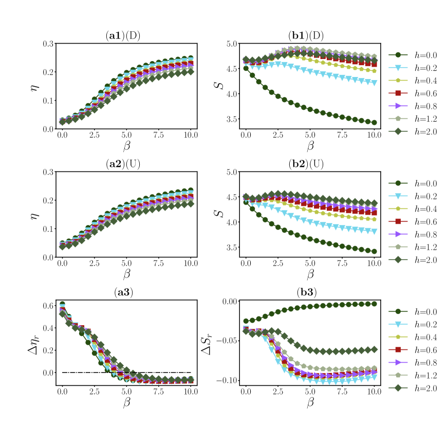
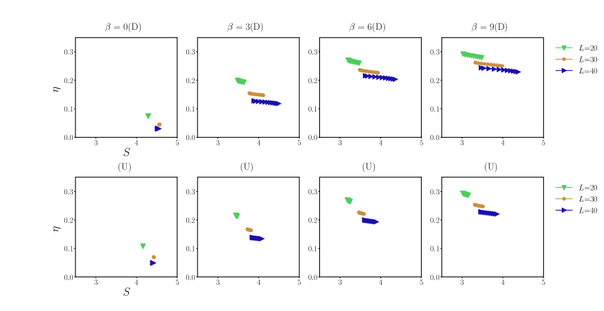
Figure (6) displays the efficiency and entropy for different values of and when the link capacities are constant, that is . Obviously the efficiency is reduced by introducing the interactions for a fixed exploration . When interactions are negligible the number of visited sites plays the main role in the efficiency, thus the efficiency is an increasing function of . For larger values of interactions, the consumed energy has the main contribution to the efficiency which could result in saturation or even reduction of the efficiency for very large . The entropy of return times changes from a decreasing to and increasing function of as the strength of interactions gets larger than about (for delta distribution) and (for uniform distribution). It is in this region that equation is satisfied for multiple values of . In words, there are movement processes which have the same uncertainty but different efficiencies . Moreover, we observe that except for very large and small , the uniform distribution of energy budgets performs better than the delta distribution in both the efficiency and the generated uncertainty in the return times.
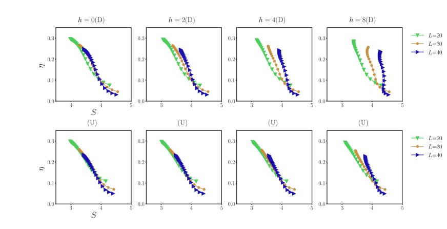
The strong effect of interactions on the efficiency and entropy can be mitigated by adjusting the link capacities according to the local populations as in Eq. 2 for . In Figs. (7) and (8) we report these quantities in terms of the parameters and , respectively. It is now around that the qualitative behavior of the entropy with changes for the delta energy distribution, see panels (b1) of the figures. Compare it with the behavior of the uniform energy distribution in panels (b2). In addition, panels (a3) show that for smaller than about efficiency of the uniform case outperforms that of the delta distribution in a large range of the interaction strengths.
Figures (9) and (10) display the size dependence of the efficiency and entropy vs the parameters and , respectively. Overall, the larger systems results in smaller efficiencies and generate more uncertainty in the return times than the smaller systems. In addition, we observe that the transition from a desirable regime (high and low ) to an undesirable one (low and high ) is sharper and occur at a larger when the initial energy budgets are the same (D) compared to the case of having a maximal energy variability (U). Moreover, the nonmonotonic behavior of appears at larger values of interactions () when the initial energies are distributed uniformly.
III Conclusion
We studied a model of interacting agents moving on a two-dimensional network using an exploration and return strategy which is governed by the available energy of the agents. We considered two distributions of initial energy budgets with very large and small energy variances but the same average energy. Energy is dissipated in the movement process with a rate that depends on the flow of particles in the links of the network. In summary, we observed that variability in initial energy helps to have in average a larger efficiency (distinct visited sites per consumed energy) when the return strategy dominates and a smaller entropy production (uncertainty in the return times) when exploration is preferred, specially in presence of strong interactions.
This study provided another example of a movement process where in average a larger entropy production results in a smaller efficiency indaco-2021 . And, in the regime of strong interactions, the efficiency can have multiple values for a given level of uncertainty in the return times. In this paper, we worked with a different model of movements and used different definitions of efficiency and entropy production from the previous works, nevertheless, the qualitative behavior of these quantities remains the same. It would be interesting to investigate analytical and numerical solutions to the continuum master equation in higher dimensions to see how much the results are affected by increasing the space dimension.
The main assumption in this work was that available energy determines the importance of exploration and return in the movements. In addition, we assumed that interactions between the agents increases the rate of energy dissipation but not the travel times of the agents. In a more realistic model the flow of particles in a link can also affect the travel or waiting times along the links. This effect can have a large impact on the values of the efficiency and uncertainty in the return times.
Acknowledgements.
This work was performed using the ALICE compute resources provided by Leiden University.References
- (1) Gonzalez, Marta C., Cesar A. Hidalgo, and Albert-Laszlo Barabasi. ”Understanding individual human mobility patterns.” nature 453, no. 7196 (2008): 779-782.
- (2) Scafetta, Nicola. ”Understanding the complexity of the Levy-walk nature of human mobility with a multi-scale cost/benefit model.” Chaos: An Interdisciplinary Journal of Nonlinear Science 21, no. 4 (2011).
- (3) Barbosa, Hugo, Marc Barthelemy, Gourab Ghoshal, Charlotte R. James, Maxime Lenormand, Thomas Louail, Ronaldo Menezes, José J. Ramasco, Filippo Simini, and Marcello Tomasini. ”Human mobility: Models and applications.” Physics Reports 734 (2018): 1-74.
- (4) Song, Chaoming, Tal Koren, Pu Wang, and Albert-László Barabási. ”Modelling the scaling properties of human mobility.” Nature physics 6, no. 10 (2010): 818-823.
- (5) Visco, Paolo, Rosalind J. Allen, Satya N. Majumdar, and Martin R. Evans. ”Switching and growth for microbial populations in catastrophic responsive environments.” Biophysical journal 98, no. 7 (2010): 1099-1108.
- (6) Bénichou, Olivier, Claude Loverdo, Michel Moreau, and Raphael Voituriez. ”Intermittent search strategies.” Reviews of Modern Physics 83, no. 1 (2011): 81.
- (7) Pappalardo, Luca, Filippo Simini, Salvatore Rinzivillo, Dino Pedreschi, Fosca Giannotti, and Albert-László Barabási. ”Returners and explorers dichotomy in human mobility.” Nature communications 6, no. 1 (2015): 8166.
- (8) Wang, Yating, and Hanshuang Chen. ”Entropy rate of random walks on complex networks under stochastic resetting.” Physical Review E 106, no. 5 (2022): 054137.
- (9) Toole, Jameson L., Carlos Herrera-Yaqüe, Christian M. Schneider, and Marta C. González. ”Coupling human mobility and social ties.” Journal of The Royal Society Interface 12, no. 105 (2015): 20141128.
- (10) Schläpfer, Markus, Lei Dong, Kevin O’Keeffe, Paolo Santi, Michael Szell, Hadrien Salat, Samuel Anklesaria, Mohammad Vazifeh, Carlo Ratti, and Geoffrey B. West. ”The universal visitation law of human mobility.” Nature 593, no. 7860 (2021): 522-527.
- (11) Riccardo, Gallotti, Bazzani Armando, and Rambaldi Sandro. ”Towards a statistical physics of human mobility.” International Journal of Modern Physics C 23, no. 09 (2012): 1250061.
- (12) Barthelemy, Marc. ”The statistical physics of cities.” Nature Reviews Physics 1, no. 6 (2019): 406-415.
- (13) Bettencourt, Luís MA. ”Introduction to urban science: evidence and theory of cities as complex systems.” (2021).
- (14) Batty, Michael. ”Defining urban science.” Urban Informatics (2021): 15-28.
- (15) Rybski, Diego, and Marta C. González. ”Cities as complex systems—Collection overview.” Plos one 17, no. 2 (2022): e0262964.
- (16) Chowell, Gerardo, James M. Hyman, Stephen Eubank, and Carlos Castillo-Chavez. ”Scaling laws for the movement of people between locations in a large city.” Physical Review E 68, no. 6 (2003): 066102.
- (17) Brockmann, Dirk, Lars Hufnagel, and Theo Geisel. ”The scaling laws of human travel.” Nature 439, no. 7075 (2006): 462-465.
- (18) Vespignani, Alessandro. ”Modelling dynamical processes in complex socio-technical systems.” Nature physics 8, no. 1 (2012): 32-39.
- (19) Xu, Yanyan, Luis E. Olmos, David Mateo, Alberto Hernando, Xiaokang Yang, and Marta C. Gonzalez. ”Urban Dynamics Through the Lens of Human Mobility.” arXiv preprint arXiv:2305.16996 (2023).
- (20) Phithakkitnukoon, Santi, Zbigniew Smoreda, and Patrick Olivier. ”Socio-geography of human mobility: A study using longitudinal mobile phone data.” PloS one 7, no. 6 (2012): e39253.
- (21) Kitamura, Ryuichi, Cynthia Chen, Ram M. Pendyala, and Ravi Narayanan. ”Micro-simulation of daily activity-travel patterns for travel demand forecasting.” Transportation 27 (2000): 25-51.
- (22) Peng, Chengbin, Xiaogang Jin, Ka-Chun Wong, Meixia Shi, and Pietro Liò. ”Collective human mobility pattern from taxi trips in urban area.” PloS one 7, no. 4 (2012): e34487.
- (23) Nagel, Kai, and Maya Paczuski. ”Emergent traffic jams.” Physical Review E 51, no. 4 (1995): 2909.
- (24) Wang, Pu, Timothy Hunter, Alexandre M. Bayen, Katja Schechtner, and Marta C. González. ”Understanding road usage patterns in urban areas.” Scientific reports 2, no. 1 (2012): 1001.
- (25) Rozenfeld, Hernán D., Diego Rybski, José S. Andrade Jr, Michael Batty, H. Eugene Stanley, and Hernán A. Makse. ”Laws of population growth.” Proceedings of the National Academy of Sciences 105, no. 48 (2008): 18702-18707.
- (26) Fibich, Gadi, and Amit Golan. ”Diffusion of new products with heterogeneous consumers.” Mathematics of Operations Research 48, no. 1 (2023): 257-287.
- (27) Pastor-Satorras, Romualdo, Claudio Castellano, Piet Van Mieghem, and Alessandro Vespignani. ”Epidemic processes in complex networks.” Reviews of modern physics 87, no. 3 (2015): 925.
- (28) Chaintreau, Augustin, Pan Hui, Jon Crowcroft, Christophe Diot, Richard Gass, and James Scott. ”Impact of human mobility on opportunistic forwarding algorithms.” IEEE Transactions on Mobile Computing 6, no. 6 (2007): 606-620.
- (29) Horner, Mark W. ”Extensions to the concept of excess commuting.” Environment and Planning A: Economy and Space 34, no. 3 (2002): 543-566.
- (30) Gastner, Michael T., and Mark EJ Newman. ”Shape and efficiency in spatial distribution networks.” Journal of Statistical Mechanics: Theory and Experiment 2006, no. 01 (2006): P01015.
- (31) Dong, Lei, Ruiqi Li, Jiang Zhang, and Zengru Di. ”Population-weighted efficiency in transportation networks.” Scientific reports 6, no. 1 (2016): 26377.
- (32) Bellocchi, Leonardo, Nikolas Geroliminis, and Vito Latora. ”Dynamical efficiency in multilayer transportation network.” In 18th Swiss transport Research Conference. 2018.
- (33) Biazzo, Indaco, Bernardo Monechi, and Vittorio Loreto. ”General scores for accessibility and inequality measures in urban areas.” Royal Society open science 6, no. 8 (2019): 190979.
- (34) Barthelemy, Marc. ”Optimal transportation networks and network design.” In Spatial Networks: A Complete Introduction: From Graph Theory and Statistical Physics to Real-World Applications, pp. 373-405. Cham: Springer International Publishing, 2022.
- (35) Kölbl, Robert, and Dirk Helbing. ”Energy laws in human travel behaviour.” New Journal of Physics 5, no. 1 (2003): 48.
- (36) Boyer, D., O. Miramontes, and H. Larralde. ”Lévy-like behaviour in deterministic models of intelligent agents exploring heterogeneous environments.” Journal of Physics A: Mathematical and Theoretical 42, no. 43 (2009): 434015.
- (37) Wang, Weiying, and Toshihiro Osaragi. ”Daily Human Mobility: A Reproduction Model and Insights from the Energy Concept.” ISPRS International Journal of Geo-Information 11, no. 4 (2022): 219.
- (38) Kölbl, Robert, and Martin Kozek. ”A physiological model of human mobility: A global study.” Humanities and Social Sciences Communications 8, no. 1 (2021): 1-14.
- (39) Biazzo, Indaco, and Abolfazl Ramezanpour. ”Efficiency and irreversibility of movements in a city.” Scientific reports 10, no. 1 (2020): 4334.
- (40) Biazzo, Indaco, Mohsen Ghasemi Nezhadhaghighi, and Abolfazl Ramezanpour. ”Entropy production of selfish drivers: implications for efficiency and predictability of movements in a city.” Journal of Physics: Complexity 2, no. 3 (2021): 035026.
- (41) Li, Ruiqi, Lei Dong, Jiang Zhang, Xinran Wang, Wen-Xu Wang, Zengru Di, and H. Eugene Stanley. ”Simple spatial scaling rules behind complex cities.” Nature communications 8, no. 1 (2017): 1841.
- (42) U. S. B. of Public Roads 1964 Traffic Assignment Manual for Application with a Large, High Speed Computer vol 2 (Washington, DC:US Department of Commerce, Bureau of Public Roads, Office of Planning, Urban Planning Division, U.S. Government Printing Office)
- (43) Huntsinger, Leta F., and Nagui M. Rouphail. ”Bottleneck and queuing analysis: Calibrating volume–delay functions of travel demand models.” Transportation research record 2255, no. 1 (2011): 117-124.
- (44) Metzler, Ralf, and Joseph Klafter. ”The random walk’s guide to anomalous diffusion: a fractional dynamics approach.” Physics reports 339, no. 1 (2000): 1-77.
- (45) Dvoretzky, A., and P. Erdös. ”Proceedings of the second Berkeley symposium on mathematical statistics and probability.” (1951): 353-367.