Abstract

Recommender Systems (RSs) are pivotal in diverse domains such as e-commerce, music streaming, and social media. This paper conducts a comparative analysis of prevalent loss functions in RSs: Binary Cross-Entropy (BCE), Categorical Cross-Entropy (CCE), and Bayesian Personalized Ranking (BPR). Exploring the behaviour of these loss functions across varying negative sampling settings, we reveal that BPR and CCE are equivalent when one negative sample is used. Additionally, we demonstrate that all losses share a common global minimum. Evaluation of RSs mainly relies on ranking metrics known as Normalized Discounted Cumulative Gain (NDCG) and Mean Reciprocal Rank (MRR). We produce bounds of the different losses for negative sampling settings to establish a probabilistic lower bound for NDCG. We show that the BPR bound on NDCG is weaker than that of BCE, contradicting the common assumption that BPR is superior to BCE in RSs training. Experiments on five datasets and four models empirically support these theoretical findings. Our code is available at https://anonymous.4open.science/r/recsys_losses.

1 Introduction

Recommender Systems (RSs) are information filtering systems made to predict a user’s preference or potential interest in a specific item quickly and accurately. These systems are widely used in various industries, such as entertainment, e-commerce, and social media. The evaluation of these systems often relies on metrics such as Normalized Discounted Cumulative Gain (NDCG) (Järvelin and Kekäläinen,, 2002), and Mean Reciprocal Rank (MRR) that measures the effectiveness of a model in presenting results in an order that reflects relevance to the user. A RSs that maximizes NDCG (MRR) gives the highest score to the next item the user is going to interact with, called the target or positive item, and lower scores to the other items in the catalogue. A common approach in RSs, especially those based on implicit feedback (e.g. clicks), is to treat user-selected items as positive and consider all other items in the catalogue as negative. However, since a catalogue can contain hundreds of millions of items, this method leads to computationally prohibitive models. Thus, ranking losses learn to discriminate a user’s positive item from a single negative item or a limited set of negative items, i.e. a small fraction of negative interactions compared to the total. Different negative sampling strategies have been proposed (Chen et al.,, 2022; Ding et al.,, 2020; Lian et al.,, 2020; Liu and Wang,, 2023; Zhang et al.,, 2013; Zhao et al.,, 2023; Zhu et al.,, 2022; Zhuo et al.,, 2022). We focus on the uniform random sampling that is used in many RSs like Caser (Tang and Wang,, 2018), SASRec (Kang and McAuley,, 2018), and GRU4Rec (Hidasi et al.,, 2016).

We consider the most common losses that are used to train RSs: Bayesian Personalized Ranking (BPR) (Rendle et al.,, 2009), Binary Cross Entropy (BCE), Categorical Cross Entropy (CCE). Our work shows that when only one negative item is sampled, CCE and BPR are equivalent. We theoretically demonstrate that, in general, they converge to the same global optimum as BCE when the item scores are bounded. However, given the challenge of reaching a global minimum in Deep Neural Networks (DNNs), and considering that gradient descent methods generally ensure only convergence to a stationary point (Baldi and Lu,, 2012; Palagi,, 2019), we extend our study to examine the behavior of these loss functions in relation to the NDCG (MRR) in scenarios where multiple negative samples are considered for each target item. We aim to better understand these loss behaviors for item recommendation. First, we identify distinct lower bounds for BCE, CCE, and BPR. Using these bounds, we show theoretically that optimizing these loss functions is equivalent to maximizing NDCG (MRR) when considering all items in the loss function. However, this statement turns out to be valid in probabilistic terms when negative sampling is adopted. Specifically, we establish probabilistic lower bounds that each loss provides on the ranking metrics. Although the probabilities of these losses being upper bounds of the ranking metrics are not directly comparable, we can analyze and compare worst-case scenarios, i.e. the smallest probabilities, demonstrating that the CCE bound on NDCG is weaker than that of BPR, which in turn is weaker than that of BCE. After several epochs, these bounds become robust enough to enhance the model’s ranking capabilities as item representations become better distributed in the latent space.

We further conduct experiments to show that our theoretical analysis is consistent with empirical evidence. We use the presented losses to train both sequential RSs like SASRec (Kang and McAuley,, 2018) and GRU4Rec (Hidasi et al.,, 2016), and non sequential RSs like Neural Collaborative Filtering (NCF) (He et al.,, 2017) and LightGNN (He et al.,, 2020) on five different datasets (MovieLens-1M, Amazon Beauty, FourSquare NYC, Amazon Books and Yelp).

The primary contributions of our work are detailed as follows:

1. We prove that CCE and BPR are equivalent when used on samples containing a single positive and a single negative item per user.

2. We prove that using the three losses leads to obtaining the same global minimum when scores are bounded.

3. We show that minimizing BCE, CCE, and BPR is equivalent to maximizing a lower NDCG (MRR) bound. We also derive probabilistic lower bounds when using negative sampling.

4. We show that, in edge cases, the CCE bound on NDCG is weaker than that of BPR that is in turn weaker than that of BCE.

5. We show that our theoretical analysis is consistent with empirical evidence, particularly in later training stages when the losses optimize a meaningful bound to NDCG (MRR).

To the best of our knowledge, no previous study has formally proven the relationships among BCE, BPR and CCE in recommendation. Therefore, this is the first paper to address the following important research question: what is the effect of the optimization process on NDCG (and MRR) when using BCE, CCE, or BPR losses, and is it possible to state which loss is better than the others?

2 Related work

RSs focuses on understanding dynamic user interests through item interactions. A detailed coverage of the related work is in the supplementary material.

Negative sampling in pointwise/pairwise losses is a common approach to address this issue: models are trained using all positive interactions while sampling only a small subset of negative interactions. Consequently, models that do not incorporate sampling, like BERT4Rec, cannot be utilized. Additionally, recent studies (Petrov and Macdonald, 2023b, ; Xu et al.,, 2024) indicate that LLM-based RSs are less effective than previously believed, with BERT4Rec’s performance gains over SASRec being due to the absence of negative sampling and Softmax loss, rather than architectural differences.
BPR (Rendle et al.,, 2009) was an early effort using negative sampling to train RSs. BPR addresses model overconfidence, i.e. the tendency to predict scores almost one for all positive items, by sampling one negative item and optimizing their relative order. However, BPR aims to optimize the Area Under the Curve (AUC) metric and the Partial AUC, which isn’t ideal for ranking tasks (Rendle,, 2022; Shi et al.,, 2023).
To improve BPR, methods like WARP (Weston et al.,, 2011), LambdaRank (Burges,, 2010), LambdaFM (Yuan et al.,, 2016), adaptive item sampling (Rendle and Freudenthaler,, 2014), importance sampling (Lian et al.,, 2020) and Augmented Negative Sampling (Zhao et al.,, 2023) target hard negative samples, i.e. the most informative ones, with erroneously high scores. These methods, often relying on iterative techniques, aren’t suitable for NN-based sequential RSs, which perform well with parallel computing on GPUs but poorly with iterative methods. Hence, sequential RSs use simple heuristics like uniform random sampling (e.g. SASRec (Kang and McAuley,, 2018) ) or no negative sampling (e.g. BERT4Rec (Sun et al.,, 2019)). Other sampling techniques are: popularity-based negative sampling (Pellegrini et al.,, 2022), that showed to be beneficial for popularity-based evaluation metrics but not for full metrics; in-batch sampling (e.g. GRU4Rec (Hidasi et al.,, 2016)) that is comparable to popularity-based sampling; and a Bayesian optimal sampling rule to do unbiased negative sampling (Liu and Wang,, 2023). Given recent studies (Dallmann et al.,, 2021; Krichene and Rendle,, 2022; Petrov and Macdonald, 2023a, ) advising against sampled metrics, we focus on the simplest uniform negative sampling technique.
BCE approaches the ranking problem by treating it as a series of independent binary classification tasks. BCE evaluates each probability separately, meaning their total does not need to sum to 1. As recently showed (Petrov and Macdonald, 2023b, ), when BCE is combined with negative sampling, the model could be overconfident in predicting the probabilities of the top-ranked items, not being able to properly distinguish between them. More recently introduced losses (Petrov and Macdonald, 2023b, ; Xu et al.,, 2024) modify BCE to adjust positive score magnitudes. While they can reduce training time, they usually require additional hyperparameter tuning and lack proven theoretical superiority.
Unlike BCE, CCE addresses the ranking problem as a multi-class classification task, accounting for the probability distribution across all sampled items. The probabilities calculated by CCE sum to 1 but are higher than that from Full Softmax loss due to a smaller denominator, making CCE prone to overconfidence (Wei et al.,, 2022). However, recent findings (Wu et al.,, 2024) indicate that CCE offers model-agnostic benefits in (i) mitigating popularity bias when using in-batch sampling, (ii) mining hard negative samples, and (iii) optimizing ranking metrics. Nevertheless, it also has a drawback in inaccurately estimating score magnitudes in RSs. In terms of ranking metrics optimization, the study demonstrates that $-logDCG$ serves as a bound for CCE when all catalogue items are considered. Comparable findings are discussed in (Bruch et al.,, 2019) and in (Pu et al.,, 2024), where a link between squared loss and ranking metrics is demonstrated via a Taylor expansion of the DCG-consistent surrogate loss, specifically the softmax loss. Our theoretical examination, however, specifically delves into the correlation between loss and ranking metrics in the context of negative sampling, which adds complexity to the analysis.
Further works (Xia et al.,, 2008; Yang and Koyejo,, 2020) study other loss properties like consistency.

3 Methodology

3.1 Background

This section formally presents the recommendation problem and the notation used in the paper.

We consider a set of users $\mathcal{U}=\{1,2,\dots,n\}\subset\mathbb{N}$ and a set of items $\mathcal{I}=\{1,2,\dots,m\}\subset\mathbb{N}$. Let’s $\mathcal{D}=\{\mathcal{I}_{1},\mathcal{I}_{2},\dots,\mathcal{I}_{n}\}$ be the set of interactions, where $\mathcal{I}_{u}=\{i_{1},i_{2},\dots,i_{m_{u}}\}\subset\mathcal{I}$ represents the set of interactions for user $u$.

The core task in recommendation is to predict the interactions $\mathcal{I}_{u}$ for a given user $u$. When considering the temporal aspect of interactions, we can split $\mathcal{I}_{u}$ into two subsets: $\mathcal{I}_{u}^{x}$ and $\mathcal{I}_{u}^{y}$, where $\mathcal{I}_{u}^{x}$ are the interactions that occurred before those in $\mathcal{I}_{u}^{y}$. The recommendation task then becomes predicting the remaining unseen interactions $\mathcal{I}_{u}^{y}=\{i\in\mathcal{I}_{u}\mid i\notin\mathcal{I}_{u}^{x}\}$ given the observed interactions $\mathcal{I}_{u}^{x}\subset\mathcal{I}_{u}$ for user $u$. Further simplification can be achieved by focusing solely on predicting the most recent item $i_{u}^{+}$ that user $u$ has interacted with: given all interactions except the last one $\mathcal{I}_{u}^{x}=\mathcal{I}_{u}\setminus\{i_{u}^{+}\}$, the task is to predict this last interaction $i_{u}^{+}\in\mathcal{I}_{u}$.

To address the prediction task, RSs typically employ a representation of users and items in a latent space. We represent the user embedding table as $\mathcal{E}_{u}:\mathcal{U}\rightarrow\mathbb{R}^{d}$ and the item embedding table as $\mathcal{E}_{i}:\mathcal{I}\rightarrow\mathbb{R}^{d}$, where both map users and items, respectively, to a $d$-dimensional real vector space. The user embedding for user $u$ is denoted as $\vec{h_{u}}=\mathcal{E}_{u}(u)$ and the item embedding for item $i$ is denoted as $\vec{h_{i}}=\mathcal{E}_{i}(i)$. The interaction score between a user $u$ and item $i$ is then computed as the dot product of their embeddings: $s_{u,i}=\mathcal{E}_{u}(u)^{T}\cdot\mathcal{E}_{i}(i)=\vec{h_{u}}\cdot\vec{h_{i}}$. Given previous interactions $\mathcal{I}_{u}^{x}$ of user $u$, the user representation $\vec{h_{u}}$ can be computed using a model $\mathcal{M}$ such that $\vec{h_{u}}=\mathcal{M}(\mathcal{I}_{u}^{x})$. Ideally, the model should learn user embeddings that capture user preferences and allow for accurate interaction prediction.

However, simply maximizing the scores $s_{u,i_{u}^{+}}$ for the positive item $i_{u}^{+}$ for each user $u$ is insufficient. A trivial solution would be to set all user embeddings $\vec{h_{u}}$ and positive item embeddings $\vec{h_{i_{u}^{+}}}$ to the same vector, which would maximizes their dot-product. To address this issue, the concept of negative items is introduced. Negative items represent items that a user $u$ has not interacted with: $\mathcal{I}_{u}^{-}=\{i\in\mathcal{I}\;s.t.\;i\notin\mathcal{I}_{u}\}$. During training, the model not only aims to maximize the score for the positive item, but also aims to minimize the scores for these negative items, guiding the learning process towards meaningful user and item representations.

3.1.1 Losses

Binary Cross-Entropy (BCE), typically applied to binary classification, can be adapted to recommendation by considering the positive item label as $1$ and negative items as $0$. The loss function is formulated as:

$$\mathcal{L}_{BCE} =-\sum_{u=1}^{U}\ell_{BCE}^{u}$$

$$\ell_{BCE}^{u} =\log\;\sigma\left(s_{u,i_{u}^{+}}\right)+\sum_{i\in\mathcal{I}_{u}^{-}}\log\left(1-\sigma\left(s_{u,i}\right)\right)$$

which, considering a single user, can be rewritten as:

$$\ell_{BCE} =log\left(1+e^{-s_{+}}\right)+\sum_{i\in\mathcal{I}^{-,K}}log\left(1+e^{s_{i}}\right)$$ (1)

Categorical Cross-Entropy (CCE) is commonly employed for multiclass classification:

$$\mathcal{L}_{CCE} =-\sum_{u=1}^{U}\ell_{CCE}^{u}$$

$$\ell_{CCE}^{u}=log\left(\frac{e^{s_{u,i_{u}^{+}}}}{e^{s_{u,i_{u}^{+}}}+\sum_{i\in\mathcal{I}_{u}^{-}}e^{s_{u,i}}}\right)$$

which, considering a single user, can be rewritten as:

$$\ell_{CCE} =log\left(1+\sum_{i\in\mathcal{I}^{-,K}}e^{\left(s_{i}-s_{+}\right)}\right)$$ (2)

Bayesian personalized ranking (BPR) is a pairwise ranking loss derived from the maximum posterior estimator. We present it here without its $L2$ weight normalization.

$$\mathcal{L}_{BPR} =-\sum_{u=1}^{U}\ell_{BPR}^{u} \ell_{BPR}^{u}=\sum_{i\in\mathcal{I}_{u}^{-}}log\;\sigma\left(s_{u,i_{u}^{+}}-s_{u,i}\right)$$ (3)

which, considering a single user, can be rewritten as:

$$\ell_{BPR} =\sum_{i\in\mathcal{I}^{-,K}}log\left(1+e^{\left(s_{i}-s_{+}\right)}\right)$$ (4)

Since the losses can be separated by user, we simplify the notation by omitting the user index $u$ whenever unambiguous. This replaces $s_{u,i_{u}^{+}}$ with $s_{+}$ and $s_{u,i}$ with $s_{i}$.

3.1.2 Metrics

Since the recommendation task involves ranking items, the crucial measure is the rank $r_{+}=|\{i:s_{i}\geq s_{+},i\in\mathcal{I^{-}}\}|$ of the positive item. This value represents the number of items (including itself) with scores greater than or equal to the positive item’s score $s_{+}$.

This value is part of various metrics. One of the most common metrics in recommendation is the Normalized Discounted Cumulative Gain (NDCG), which incorporates the graded relevance of items at different positions in the ranking:

$$NDCG(r_{+})=\frac{1}{log_{2}(1+r_{+})}$$ (5)

Another ranking metric valuable for evaluating RSs is Mean Reciprocal Rank (MRR). MRR considers the reciprocal rank of the first relevant item in the recommendation list:

$$MRR(r_{+})=\frac{1}{r_{+}}$$ (6)

3.1.3 Negative sampling

While the ideal scenario involves computing the true positive item rank $r_{+}$ and the true loss value, the sheer number of negative items $|I^{-}|$ makes it infeasible to compute all scores $s_{i}$ . Instead, a subset $\mathcal{I}^{-,K}\subseteq\mathcal{I}^{-}$, with $|\mathcal{I}^{-,K}|=K$, is usually sampled for computational cost.

Negative sampling, though, introduces its own limitations. Because we only sample a subset of negative items, directly calculating the true rank is not possible. However, we can estimate the rank using an approximation $\hat{r}_{+}$. Let’s define $\Gamma^{K}$ as the set of $K$ sampled negative items with scores greater than or equal to the positive item score $s_{+}$: $\Gamma^{K}=\{i:s_{i}\geq s_{+},i\in\mathcal{I}^{-,K}\}$. The cardinality of this set provides a lower bound for the positive item rank $r_{+}$: $|\Gamma^{K}|+1=\leq r_{+}$. Another set worth considering is the set of all sampled negative items with non-negative scores: $\Gamma^{K}_{0}=\{i:s_{i}\geq 0,i\in\mathcal{I}^{-,K}\}$. This set includes hard negative items (clearly irrelevant) and marginally relevant items that the model doesn’t outright reject, suggesting they may have some relevance to the user.

3.2 Theoretical results

3.2.1 Global minimum

This section explores the theoretical properties of loss functions commonly used in RSs with negative sampling.

It can be easily seen that $\ell_{BPR}$ is equivalent to $\ell_{CCE}$ when sampling one negative item.

Proposition 1.

$\ell_{BPR}$ = $\ell_{CCE}$ if one negative item $K=1$ is sampled for each user.

Next, we present a theorem that formally states the equivalence of global minima for the three loss functions. The theorem demonstrates that when one negative item is sampled and item scores are bounded, BPR, BCE, and CCE will all achieve the same global minimum.

Proposition 2.

If $s_{+},s_{i}\in[-S,S]$ with $S\in\mathbb{R^{+}}$ then:

$$\operatorname*{arg\,min}_{s_{+}}\ell_{BCE}=\operatorname*{arg\,min}_{s_{+}}\ell_{BPR}=\operatorname*{arg\,min}_{s_{+}}\ell_{CCE}=S$$

$$\operatorname*{arg\,min}_{s_{i}}\ell_{BCE}=\operatorname*{arg\,min}_{s_{i}}\ell_{BPR}=\operatorname*{arg\,min}_{s_{i}}\ell_{CCE}=-S$$

This result has significant implications for training RSs. Firstly, it suggests consistency across BPR, BCE, and CCE loss functions in this specific scenario. This simplifies the choice of loss function in practical applications, as all three lead to the same optimal solution, reducing hyperparameter tuning complexity.

However, it’s important to acknowledge limitations in applying this finding to DNNs used in RSs. RSs inherently incorporate inductive biases for generalization and the choice of the best model based on the validation set, avoids overfitting making such extreme values $S$ and $-S$ unattainable. Moreover, DNNs typically have non-convex error surfaces with numerous stationary points, including local minima with identical objective values (Palagi,, 2019). Achieving a global minimum in DNNs with nonlinear activation functions is difficult, and the gradient descent methods typically only guarantee convergence to a stationary point (Baldi and Lu,, 2012; Palagi,, 2019). Considering these limitations, in the following sections we explore how these loss functions interact with ranking metrics under negative sampling.

3.2.2 Bounds

Our goal is to achieve a deeper understanding of losses’ behaviour in the context of item recommendation. We establish lower bounds for each loss function in the negative sampling regime. These bounds will be instrumental in deriving probabilistic bounds for NDCG.

Lemma 1.

Given $\Gamma^{K}$ and $\Gamma^{K}_{0}$, we have

$$\ell_{BPR}\geq|\Gamma^{K}|\log 2 \ell_{BCE}\geq|\Gamma^{K}_{0}|\log 2$$

$$\ell_{CCE}\geq\log(|\Gamma^{K}|).$$

3.2.3 Loss ranking capability

The established bounds on the losses depend on the cardinality of sets: $\Gamma^{K}$ and $\Gamma^{K}_{0}$, which are influenced by the negative sampling method. Here, we introduce a way of computing these probabilities.

Lemma 2.

Let consider the sets $\Gamma^{K}$ and $\Gamma^{K}_{0}$. If the $K$ negative items are uniformly sampled without replacement from the set $I^{-}$ of all negative items, then $|\Gamma^{K}|$ and $|\Gamma^{K}_{0}|$ are described by two hypergeometrics:

$$|\Gamma^{K}|\sim Hypergeometric\left(|I^{-}|,|\Gamma|,K\right)$$

$$|\Gamma^{K}_{0}|\sim Hypergeometric\left(|I^{-}|,|\Gamma_{0}|,K\right)$$

The following theorem establish the minimum probability that the three losses are an upper bound on the negative logarithm of NDCG. This tells us than minimising a loss leads to maximising the NDCG.

Theorem 1.

When uniformly sampling $K$ negative items, we have:

$$\mathbb{P}(-\log\text{NDCG}(r_{+})\leq\ell_{BCE})$$

$$\geq 1-CDF_{|\Gamma^{K}_{0}|}\left(\log_{2}\left(\log_{2}(1+r_{+})\right)\right)$$ (7)

$$\mathbb{P}(-\log\text{NDCG}(r_{+})\leq\ell_{BPR})$$

$$\geq 1-CDF_{|\Gamma^{K}|}\left(\log_{2}\left(\log_{2}(1+r_{+})\right)\right)$$ (8)

$$\mathbb{P}(-\log\text{NDCG}(r_{+})\leq\ell_{CCE})$$

$$\geq 1-CDF_{|\Gamma^{K}|}\left(\log_{2}(1+r_{+})\right)$$ (9)

3.2.4 Comparing losses

This section compares the probabilistic bounds established for each loss function in their ability to upper bound $-\log(NDCG)$. We focus on the worst-case scenario, where the probability of achieving the bound is minimized.

Theorem 2.

When uniformly sampling $K$ negative items, in the worst-case scenario, and $s_{+}\geq 0$:

$$\mathbb{P}(-\log\text{NDCG}(r_{+})\leq\ell_{BCE})\geq$$

$$\mathbb{P}(-\log\text{NDCG}(r_{+})\leq\ell_{BPR})\geq$$

$$\mathbb{P}(-\log\text{NDCG}(r_{+})\leq\ell_{CCE})$$

Theorem 2 shows that the bound for BPR is inherently weaker than the bound for BCE because the corresponding term in BPR is smaller. This suggests that BPR is less likely to achieve a good bound on NDCG compared to BCE. In addition, for the same predicted rank $r_{+}$ and number of negative samples $K$, the bound probability for BPR is higher than for CCE.

As training progresses, the true rank $r_{+}$ of the positive item generally decreases, meaning that it ranks higher in relation to other items. This reduction in $r_{+}$ can decrease the size of $|\Gamma^{K}|$, which in turn influences the probability bound for the ranking model. This interplay makes it challenging to determine a definitive trend. Additionally, during training, models trained using BPR and CCE may begin to predict different values of $r_{+}$ due to their distinct optimization objectives. This difference in predicted ranks can alter the relationship between the probabilities derived from the bounds, further complicating the trend analysis.

In contrast, the BCE bound appears more favorable. The set of negative items with non-negative scores $|\Gamma_{0}|$ likely remains stable during training as item embeddings are probably uniformly distributed in latent space. Consequently if the true rank $r_{+}$ decreases, the probability of BCE achieving a good NDCG bound increases as the bound’s CDF goes down. This suggests that BCE might become a more reliable bound compared to BPR and CCE as training progresses.

3.3 Mean Reciprocal Rank

The results for MRR are analogous to those for NDCG and reported integrally in the appendix.

4 Experiments

In this section, we outline the experimental design employed to empirically validate our theoretical findings regarding recommendation loss functions under negative sampling.

4.1 Experimental setup

We follow a next-item prediction approach, aligning with established works (Hidasi et al.,, 2016; Kang and McAuley,, 2018). This signifies that the positive instance under evaluation is the next item to be predicted, which corresponds to the last item in a user’s test sequence.

Datasets. To ensure the generalizability of our results, we leverage three well-regarded real-world benchmark datasets for RSs:

• Amazon Beauty (McAuley et al.,, 2015): This dataset, on the smaller side, encompasses product reviews from 1,274 users for 1,076 items, totalling 7,113 interactions.

• Foursquare NYC (Yang et al.,, 2015): A widely adopted dataset containing check-in records within New York City, encompassing 227,42 entries.

• MovieLens 1M (Harper and Konstan,, 2015): This dataset features 1 million movie ratings from various users.

The details of the larger datasets, Yelp and Amazon Books, and the related results of experiments conducted on these datasets are given in the supplementary material.

Baselines. For a thorough evaluation, we incorporate two well-established, state-of-the-art RSs: (i) GRU4Rec (Hidasi et al.,, 2016) that leverages a Gated Recurrent Unit architecture for recommendation; (ii) SASRec (Kang and McAuley,, 2018) that employs a self-attention mechanism for recommendation tasks.

Results for non-sequential RSs, NCF and LightGCN, are presented in the supplementary material.

Losses. We evaluate the performance of the three introduced loss functions: BCE, BPR, and CCE.

Negative Sampling. We consider different number of uniformly sampled negative items per sample. In particular, the considered values are within the set $\{1,2,5,20,50,100\}$.

Hyperparameter Settings For consistency across all experiments, we utilize the following hyperparameters: Embedding Size: 64; Input Sequence Length: 200; Batch Size: 128; Optimizer: Adam; Learning Rate: 0.001; Maximum Training Epochs: 600.
These hyperparameter selections were established based on prevailing practices within the RSs domain, as evidenced in prior works like (Hidasi et al.,, 2016; Kang and McAuley,, 2018).

4.2 Empirical results

Due to space constraints, we present the results only for the ML-1M dataset. The results for the other datasets can be found in the appendix. Similar considerations to those drawn in this section also apply to the other datasets.

4.2.1 Number of negatives comparison

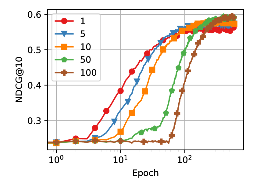
(a) BCE

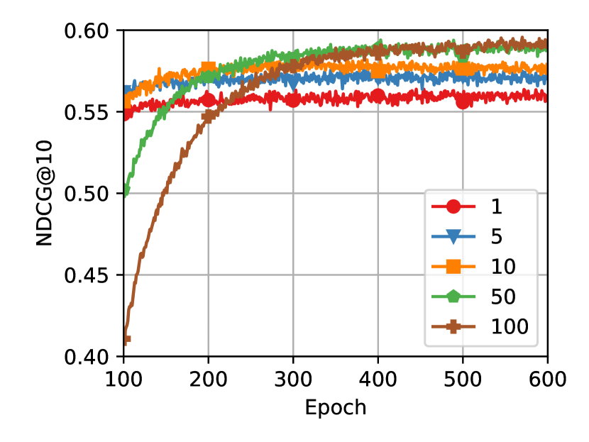
(b) BCE - End

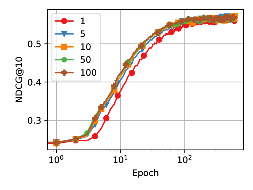
(c) BPR

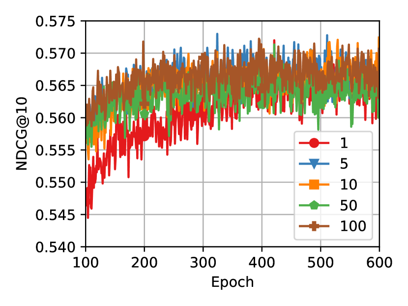
(d) BPR - End

(e) CCE

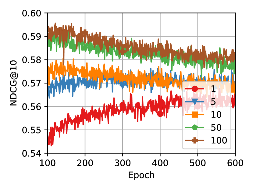
(f) CCE - End

Figure 1: GRU4Rec NDCG@10 during training changing number of negative items and loss on ML-1M dataset.

(a) BCE

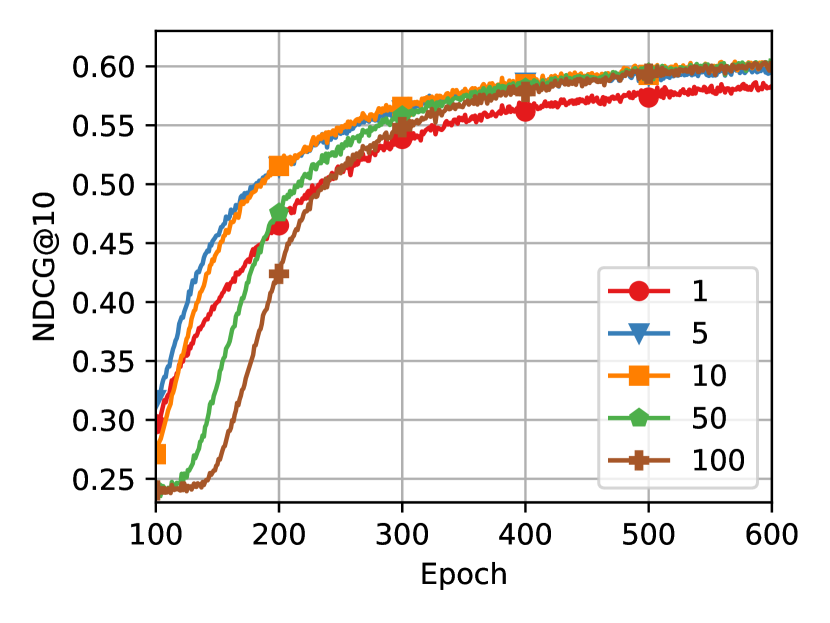
(b) BCE - End

(c) BPR

(d) BPR - End

(e) CCE

(f) CCE - End

Figure 2: SASRec NDCG@10 during training changing number of negative items and loss on ML-1M dataset.

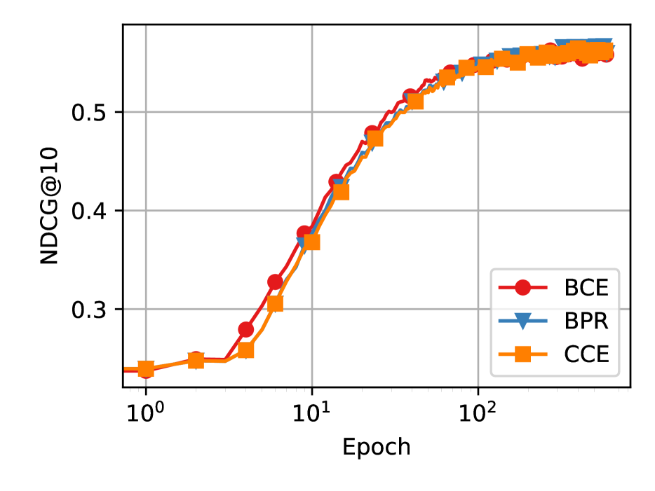
(a) GRU4Rec

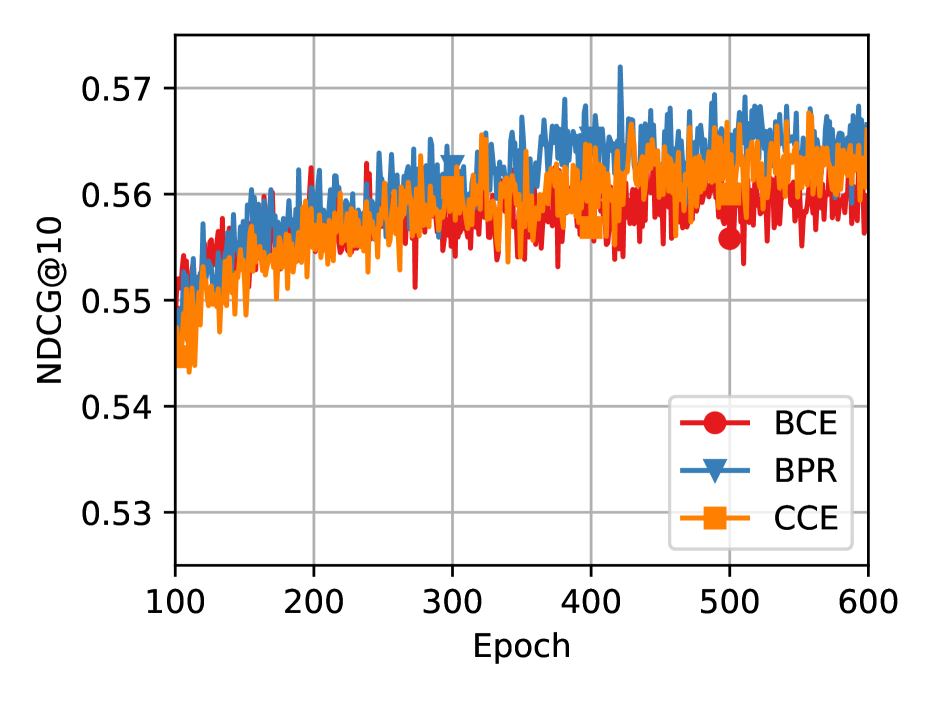
(b) GRU4Rec - End

(c) SASRec

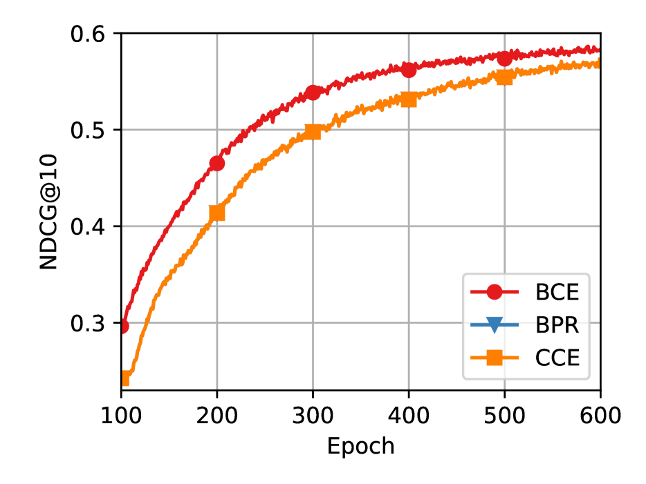
(d) SASRec - End

Figure 3: SASRec and GRU4Rec NDCG@10 during training, using 1 negative item and changing loss on ML-1M dataset.

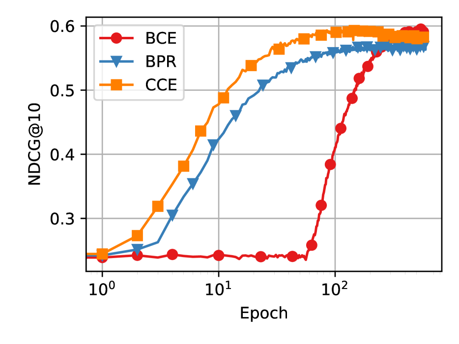
(a) GRU4Rec

(b) GRU4Rec - End

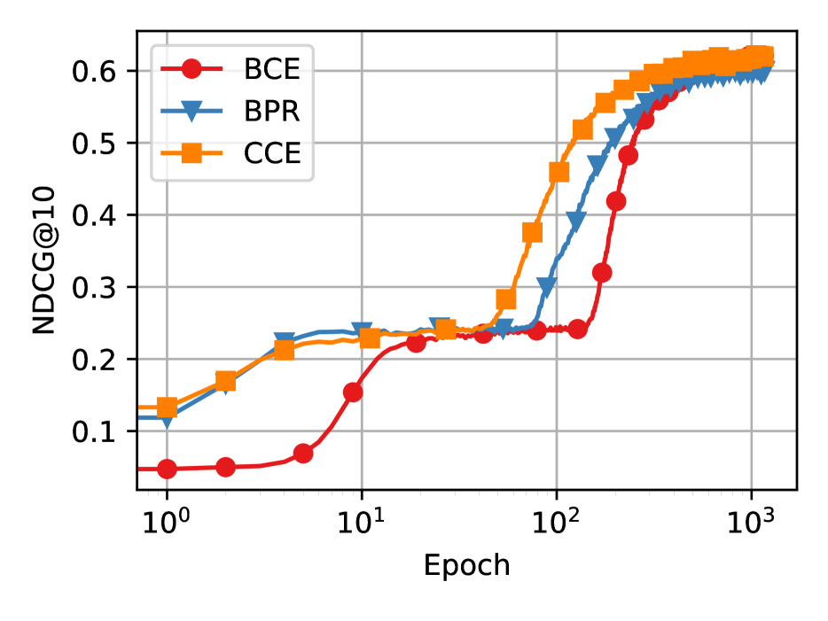
(c) SASRec

(d) SASRec - End

Figure 4: SASRec and GRU4Rec NDCG@10 during training, using 100 negative items and changing loss on ML-1M dataset.

Figs. 1 and 2 visualize the results for GRU4Rec and SASRec. The results show NDCG@10 as a function of training epochs and the number of negative items, for the three losses. We also present a zoom on the last epochs to better assess the situation in this important training phase.

For BCE, we can observe that in the early training epochs, using fewer negatives leads to better results. In particular, NDCG@10 exhibits an initial plateau that extends the more negatives there are; so much so that when $100$ are used, GRU4Rec does not show improvements in the metric until almost epoch $100$. This could be due to the fact that the model is focusing too much on the negatives and too little on the positive item. In the initial training stages, the model is still learning to distinguish between relevant and irrelevant items and the embedding representations in the latent space are poor. This is even more challenging when more negative items and only one positive item are considered.

The final part of the training shows a different situation. In fact, even though the increase in the metric is postponed for many negatives, the rise is faster, so much so that the final metric benefits from the use of more negatives: the best final metrics are obtained when $100$ negatives are used. This is likely because, once the model is trained, it is more difficult to do meaningful sampling using only one negative, while it is easier to draw items with scores higher than the positive one if more are used.

BPR behaves similarly at the end of training, but shows that using more negatives is even better initially. Our hypothesis is that in BPR the positive item is used for the loss calculation paired with each negative, so it is effectively weighted the same number of times as the negatives.

Finally, CCE shows results similar to BPR, with the use of more negatives improving both the final and initial phase of training. This is the only model where it is possible to notice a slight difference between the two models, GRU4Rec and SASRec, specifically in the early training epochs, where using $5$ or $10$ negatives seems to be better than using either $1$ or $100$, even if the difference is small.

CCE is the only case where we observe some model overfitting, especially with more negatives.

We can conclude that, in general, the use of more negatives is almost always advantageous, especially for the end performance of the models. However, since the use of a single negative is a special case of interest, the next section will compare the losses with one negative and $100$ negatives, the two limiting cases of the analysis we have carried out.

4.2.2 Losses Comparison

Figs. 3 and 4 visualize the results for using 1 and 100 negative items, respectively. The results show NDCG@10 as a function of training epochs and the different loss used. We also present a zoom on the last epochs to better assess the situation in this important training phase.

From Fig. 3, the one in the case of using one negative, we can see that the results for BPR and CCE are actually identical, as theoretically demonstrated in the previous sections. This is exact for SASRec, while on GRU4Rec the results of the two are slightly different, a difference probably due to machine approximation (since in the code they remain implemented in their original formula).

We notice a different trend between GRU4Rec and SASRec, where for the former, in the early epochs, BCE performs slightly better than BPR/CCE, while on SASRec the opposite happens. In the final epochs, BCE is performing better on SASRec, while the difference between the three losses is less pronounced for GRU4Rec.

With 100 negatives, instead, we notice an opposite trend, with CCE dominating BPR, except for a few epochs on SASrec, which in turn gets better results than BCE. The latter, however, manages to surpass the other two losses in the very last training epochs. This is in line with what was said previously, namely that with many negatives it is more difficult for BCE to provide a meaningful bound to the NDCG at the beginning of training, but it manages to provide a better one at the end of training.

5 Conclusions

In this paper, we provided a comprehensive theoretical analysis of BCE, CCE, and BPR losses in the context of RSs. We have shown that optimizing these losses consistently maximizes NDCG and MRR metrics, always when all negative items are considered and probabilistically when only a subset is used. We studied the impact of uniform negative sampling when different numbers of negative items are considered. Our findings revealed that BPR and CCE share the same functional form when one negative item is considered. We first proved that the three losses share the same global minimum. Secondly, we proved that CCE and BPR bounds on ranking metrics are generally weaker than those provided by BCE, especially in the later stages of training. Experimental results across various datasets validated our theoretical insights. This work advances our understanding of how different loss functions impact RSs performance, providing a foundation for future model training and evaluation improvements. Future research could investigate the impact of various negative sampling strategies on loss performance, as the current theorems are valid only with uniform sampling. An open problem is extending our analysis to the multi-user scenario where an item can be positive for one user but negative for another, where the loss optimization becomes more complex and difficult to study. Future work could explore other losses’ properties for a more complete understanding and use the results and insights obtained to develop a new and more effective loss function.

Limitations. This paper compares loss functions under the worst-case scenario, where the probability that these losses serve as a bound for ranking metrics is minimized. Additionally, our analysis assumes that the score for the target item is non-negative, a condition likely to occur during later stages of model training but probably not in the early phases of training. Moreover, our analysis doesn’t directly compare the tightness of the bounds each loss function provides for NDCG. Therefore, the observed advantage of BCE over other losses might not be universally valid.

Supplementary material

Appendix A Related work (cont.)

RSs aim to capture the compatibility between users and items by leveraging historical user interactions, such as purchases, likes and clicks. Feedback from users can be explicit, like ratings, or implicit, like clicks. Interpreting implicit feedback and understanding how to model unobserved interactions present challenges. To handle this, point-wise (Hu et al.,, 2008) and pair-wise Rendle et al., (2009) methods have been proposed. Collaborative filtering (CF) (Hu et al.,, 2008) methods, including user-based and item-based techniques, have long been popular for their straightforward implementation and ability to effectively capture patterns in user-item interactions. More sophisticated matrix factorization methods, such as Singular Value Decomposition (SVD) (Koren et al.,, 2009) and Non-negative Matrix Factorization (NMF) (Lee and Seung,, 1999), have advanced CF by generating compact, latent representations that allow for more precise modeling of user and item preferences.
Beyond CF, neural network-based recommender systems, particularly those leveraging deep learning, have gained prominence for their ability to capture complex, non-linear relationships within data. Sequential RSs focuses on understanding dynamic user interests through sequences of item interactions. Early approaches such as GRU4Rec (Hidasi et al.,, 2016) and Neural Attentive Session-based Recommendation (NARM)(Li et al.,, 2017) used Recurrent Neural Networks (RNNs) for sequence modeling. Concurrently, Neural Collaborative Filtering (NCF) (He et al.,, 2017) and Caser (Tang and Wang,, 2018) were introduced. More recently, the Transformer architecture (Vaswani et al.,, 2017) has gained popularity in RSs due to its parallel processing capabilities and superior performance. For instance, SASRec (Kang and McAuley,, 2018) utilizes a unidirectional self-attention mechanism, while BERT4Rec (Sun et al.,, 2019) and Transformers4Rec (de Souza Pereira Moreira et al.,, 2021) employ bidirectional self-attention for sequential recommendation tasks. $S^{3}$-Rec (Zhou et al.,, 2020) advances beyond masking techniques by pre-training on four self-supervised tasks to enhance data representation. Graph-based approaches, such as LightGCN (He et al.,, 2020), have also been effective in modeling higher-order relationships in recommendation data, using graph convolutions to capture structural dependencies between users and items. Lately TIGER (Rajput et al.,, 2023) has been proposed that directly predicts the Semantic ID of the next item using Generative Retrieval, bypassing the need for Approximate Nearest Neighbor search in a Maximum Inner Product Search (MIPS) space.
It is important to note that next-token prediction for Large Language Model (LLM)-based RSs pre-training and fine-tuning employs a cross-entropy loss with a Full Softmax over the entire corpus. However, due to the vast size of item catalogues in many real-world applications, using this loss becomes computationally prohibitive.

Appendix B Global minimum

Proposition 3.

$\ell_{BPR}$ = $\ell_{CCE}$ if $K=1$

Proof.

If $K=1$, then we can lose the summation on both losses, getting:

$$\ell_{BPR}=log\left(1+e^{\left(s_{i}-s_{+}\right)}\right) \ell_{CCE}=log\left(1+e^{\left(s_{i}-s_{+}\right)}\right)$$

∎

Proposition 2 in the main paper appears in the appendix as Propositions 4, 5 and 6.

Proposition 4.

Let us consider the $\ell_{BPR}$ and let’s bound the scores $-S\leq s_{+},s_{i}\leq S$. We have that:

$$\operatorname*{arg\,min}_{s_{+}}\ell_{BPR}=S \operatorname*{arg\,min}_{s_{i}}\ell_{BPR}=-S$$

Proof.

We have

$$\operatorname*{arg\,min}_{s_{+}}\ell_{BPR}=\operatorname*{arg\,min}_{s_{+}}\sum_{i\in\mathcal{I}^{-,K}}log\left(1+e^{\left(s_{i}-s_{+}\right)}\right)=\operatorname*{arg\,min}_{s_{+}}-s_{+}=\max_{s_{+}}s_{+}=S$$

$$\operatorname*{arg\,min}_{s_{i}}\ell_{BPR}=\operatorname*{arg\,min}_{s_{i}}\sum_{i\in\mathcal{I}^{-,K}}log\left(1+e^{\left(s_{i}-s_{+}\right)}\right)=\operatorname*{arg\,min}_{s_{i}}s_{i}=\min_{s_{i}}s_{i}=-S$$

∎

Proposition 5.

Let us consider the $\ell_{BCE}$ and let’s bound the scores $-S\leq s_{+},s_{i}\leq S$. We have that:

$$\operatorname*{arg\,min}_{s_{+}}\ell_{BCE}=S \operatorname*{arg\,min}_{s_{i}}\ell_{BCE}=-S$$

Proof.

We have

$$\operatorname*{arg\,min}_{s_{+}}\ell_{BCE}=\operatorname*{arg\,min}_{s_{+}}log\left(1+e^{-s_{+}}\right)+\sum_{i\in\mathcal{I}^{-,K}}log\left(1+e^{s_{i}}\right)=\operatorname*{arg\,min}_{s_{+}}-s_{+}=\max_{s_{+}}s_{+}=S$$

$$\operatorname*{arg\,min}_{s_{i}}\ell_{BCE}=\operatorname*{arg\,min}_{s_{i}}log\left(1+e^{-s_{+}}\right)=\operatorname*{arg\,min}_{s_{i}}s_{i}=\min_{s_{i}}s_{i}=-S$$

∎

Proposition 6.

Let us consider the $\ell_{CCE}$ and let’s bound the scores $-S\leq s_{+},s_{i}\leq S$. We have that:

$$\operatorname*{arg\,min}_{s_{+}}\ell_{CCE}=S \operatorname*{arg\,min}_{s_{i}}\ell_{CCE}=-S$$

Proof.

We have

$$\operatorname*{arg\,min}_{s_{+}}\ell_{CCE}=\operatorname*{arg\,min}_{s_{+}}log\left(1+\sum_{i\in\mathcal{I}^{-,K}}e^{\left(s_{i}-s_{+}\right)}\right)=\operatorname*{arg\,min}_{s_{+}}-s_{+}=\max_{s_{+}}s_{+}=S$$

$$\operatorname*{arg\,min}_{s_{i}}\ell_{CCE}=\operatorname*{arg\,min}_{s_{i}}log\left(1+\sum_{i\in\mathcal{I}^{-,K}}e^{\left(s_{i}-s_{+}\right)}\right)=\operatorname*{arg\,min}_{s_{i}}s_{i}=\min_{s_{i}}s_{i}=-S$$

∎

Appendix C Loss bounds

Lemma 1 in the main paper appears in the appendix as Lemmas 3, 4 and 5.

Lemma 3.

Given $\Gamma^{K}$, for BPR loss we have

$$\ell_{BPR}\geq|\Gamma^{K}|\log 2.$$

Proof.

According to the definition of BPR, it follows that

$$\ell_{BPR} =\sum_{i\in\mathcal{I^{-,K}}}\log\left(1+e^{(s_{i}-s_{+})}\right)$$

$$=\sum_{i\in\Gamma^{K}}\log\left(1+e^{(s_{i}-s_{+})}\right)+\sum_{i\notin\Gamma^{K}}\log\left(1+e^{(s_{i}-s_{+})}\right)$$

$$\geq\sum_{i\in\Gamma^{K}}\log\left(1+e^{(s_{i}-s_{+})}\right)$$

$$\geq|\Gamma^{K}|\log 2$$

∎

Lemma 4.

Given $\Gamma^{K}_{0}$, for BCE loss we have:

$$\ell_{BCE}\geq|\Gamma^{K}_{0}|\log 2.$$

Proof.

According to the definition of BCE, it follows that

$$\ell_{BCE} =log\left(1+e^{-s_{+}}\right)+\sum_{i\in\mathcal{I}^{-,K}}log\left(1+e^{s_{i}}\right)$$

$$=\log\left(1+e^{-s_{+}}\right)+\sum_{i\in\Gamma^{K}_{0}}\log\left(1+e^{s_{i}}\right)+\sum_{i\notin\Gamma^{K}_{0}}\log\left(1+e^{s_{i}}\right)$$

$$\geq\sum_{i\in\Gamma^{K}_{0}}\log\left(1+e^{s_{i}}\right)$$

$$\geq|\Gamma^{K}_{0}|\log 2$$

∎

Lemma 5.

Given $\Gamma^{K}$, for CCE loss we have

$$\ell_{CCE}\geq\log(|\Gamma^{K}|).$$

Proof.

According to the definition of CCE, it follows that

$$\ell_{CCE} =log\left(1+\sum_{i\in\mathcal{I}^{-,K}}e^{\left(s_{i}-s_{+}\right)}\right)$$

$$=\log\left(1+\sum_{i\in\Gamma^{K}}e^{(s_{i}-s_{+})}+\sum_{i\notin\Gamma^{K}}e^{(s_{i}-s_{+})}\right)$$

$$\geq\log\left(\sum_{i\in\Gamma^{K}}e^{(s_{i}-s_{+})}\right)$$

$$\geq\log\left(|\Gamma^{K}|\right)$$

∎

Appendix D Ranking capability

Lemma 2 in the main paper appears in the appendix as Lemma 6.

Lemma 6.

Let consider the sets $\Gamma^{K}$ and $\Gamma^{K}_{0}$. The $K$ negative items are uniformly sampled from the set $I^{-}$ of all negative items. Let $\Gamma=\{i\in I^{-}:s_{i}>s_{+}\}$ be the set of all negative items meeting the condition of the set $\Gamma^{K}$, with the cardinality $|\Gamma|=r_{+}-1$. Let $\Gamma_{0}=\{i\in I^{-}:s_{i}>s_{+}\}$ be the set of all items meeting the condition of the set $\Gamma^{K}_{0}$, with the cardinality $|\Gamma_{0}|$. If the negative items are drawn without replacement, the two discrete random variables are described by two hypergeometrics:

$$|\Gamma^{K}|\sim Hypergeometric\left(|I^{-}|,|\Gamma|,K\right)\;\;\;|\Gamma^{K}_{0}|\sim Hypergeometric\left(|I^{-}|,|\Gamma_{0}|,K\right)$$

Proof.

The hypergeometric distribution is a discrete probability distribution that describes the probability of k successes in n draws, without replacement, from a finite population of size N that contains exactly K objects with that feature, wherein each draw is either a success or a failure. In this context, the population consists of negative items, i.e. is the set $\mathcal{I^{-}}$. In both cases, items are divided into two sets: those meeting the condition of $\Gamma^{K}$ or $\Gamma^{K}_{0}$ and their respective complements. This division matches the hypergeometric distribution, where the population is split into two groups. We consider the probability of uniformly drawing a subset of $K$ negative items that meets the specific condition of the set $\Gamma$ or $\Gamma_{0}$ from the finite population, given by $\frac{|\Gamma|}{|\mathcal{I^{-}}|}$ or $\frac{|\Gamma_{0}|}{|\mathcal{I^{-}}|}$, respectively. ∎

Theorem 1 in the main paper appears in the appendix as Theorems 3, 4 and 5

Theorem 3.

Let consider the BPR loss when, for each user, we uniformly sample $K$ negative items for training. Let $\Gamma=\{i\in I^{-}:s_{i}\geq s_{+}\}$ be the set of all negative items that have a score greater or equal to the score of the positive item that is ranked $r_{+}$. Then we have

$$-log(NDCG(r_{+}))\leq\ell_{BPR}$$ (10)

with probability at least

$$1-\sum_{i=0}^{\log_{2}(\log_{2}(1+r_{+}))}\frac{\binom{|\Gamma|}{i}\binom{|\mathcal{I^{-}}|-|\Gamma|}{K-i}}{\binom{|\mathcal{I^{-}}|}{K}}$$ (11)

Proof.

According to Lemma 3 we know that

$$\ell_{BPR}\geq|\Gamma^{K}|\log 2$$

Therefore, Eq. 10 can be rewritten as:

$$P(-\log\text{NDCG}(r_{+})\leq\ell_{BPR}) \geq P\left(-\log\left(\frac{1}{\log_{2}\left(1+r_{+}\right)}\right)\leq|\Gamma^{K}|\log 2\right)$$ (12)

$$=P\left(\log_{2}\left(1+r^{+}\right)\leq 2^{|\Gamma^{K}|}\right) =P\left(|\Gamma^{K}|\geq\log_{2}\left(\log_{2}(1+r_{+})\right)\right)$$

According to Lemma 2 of the main paper, $|\Gamma^{K}|$ is an hypergeometric variable with population size $|\mathcal{I^{-}}|$, $|\Gamma^{K}|$ number of successes and $K$ number of draws. Thus, we can rewrite LABEL:eq:prob_BPR using the cumulative distribution function of an hypergeometric:

$$P\left(|\Gamma^{K}|\geq\log_{2}\left(\log_{2}(1+r_{+})\right)\right)=1-CDF_{|\Gamma^{K}|}\left(\log_{2}\left(\log_{2}(1+r_{+})\right)\right)$$

that is

$$P\left(-log(NDCG(r_{+}))\leq\ell_{BPR}\right)\geq 1-\sum_{i=0}^{\log_{2}(\log_{2}(1+r_{+}))}\frac{\binom{|\Gamma|}{i}\binom{|\mathcal{I^{-}}|-|\Gamma|}{K-i}}{\binom{|\mathcal{I^{-}}|}{K}}$$

∎

Theorem 4.

Let consider the BCE loss when, for each user, we uniformly sample $K$ negative items for training. Let $\Gamma_{0}=\{i\in I^{-}:s_{i}\geq 0\}$ be the set of all negative items that have a non-negative score. Then we have

$$-log(NDCG(r_{+}))\leq\ell_{BCE}$$ (14)

with probability at least

$$1-\sum_{i=0}^{\log_{2}(\log_{2}(1+r_{+}))}\frac{\binom{|\Gamma_{0}|}{i}\binom{|\mathcal{I^{-}}|-|\Gamma^{0}|}{K-i}}{\binom{|\mathcal{I^{-}}|}{K}}$$ (15)

Proof.

According to Lemma 4 we know that

$$\ell_{BCE}\geq|\Gamma^{K}_{0}|\log 2$$

Thus, the demonstration is equivalent to that of Theorem 4, using the set $\Gamma_{0}^{K}$ instead of $\Gamma^{K}$. ∎

Theorem 5.

Let consider the CCE loss when, for each user, we uniformly sample $K$ negative items for training. Let $\Gamma=\{i\in I^{-}:s_{i}\geq s_{+}\}$ be the set of all negative items that have a score greater or equal to the score of the positive item that is ranked $r_{+}$. Then we have

$$-log(NDCG(r_{+}))\leq\ell_{CCE}$$ (16)

with probability at least

$$1-\sum_{i=0}^{\log_{2}(1+r_{+})}\frac{\binom{|\Gamma|}{i}\binom{|\mathcal{I^{-}}|-|\Gamma|}{K-i}}{\binom{|\mathcal{I^{-}}|}{K}}$$ (17)

Proof.

According to Lemma 5 we know that

$$\ell_{CCE}\geq\log(|\Gamma^{K}|)$$

Therefore, Eq. 16 can be rewritten as follows:

$$P(-\log\text{NDCG}(r_{+})\leq\ell_{CCE}) \geq P\left(-\log\left(\frac{1}{\log_{2}\left(1+r_{+}\right)}\right)\leq\log(|\Gamma^{K}|)\right)$$ (18)

$$=P\left(|\Gamma^{K}|\geq\log_{2}(1+r_{+})\right)$$

According to Lemma 2 of the main paper, the set $\Gamma^{K}$ is an hypergeometric variable with population size $|\mathcal{I^{-}}|$, $|\Gamma^{K}|$ number of successes and $K$ number of draws. Thus, we can rewrite LABEL:eq:prob_BPR using the cumulative distribution function of an hypergeometric:

$$P\left(|\Gamma^{K}|\geq\log_{2}(1+r_{+})\right)=1-CDF_{|\Gamma^{K}|}\left(\log_{2}(1+r_{+})\right)$$

that is

$$P\left(-log(NDCG(r_{+}))\leq\ell_{CCE}\right)\geq\left(1-\sum_{i=0}^{\log_{2}(1+r_{+})}\frac{\binom{|\Gamma|}{i}\binom{|\mathcal{I^{-}}|-|\Gamma|}{K-i}}{\binom{|\mathcal{I^{-}}|}{K}}\right)$$

∎

Appendix E Losses comparative analysis

Theorem 2 in the main paper appears in the appendix as Theorem 6.

Theorem 6.

When uniformly sampling $K$ negative items, in the worst-case scenario and $s_{+}\geq 0$:

$$\mathbb{P}(-\log\text{NDCG}(r_{+})\leq\ell_{BCE})\geq\mathbb{P}(-\log\text{NDCG}(r_{+})\leq\ell_{BPR})\geq\mathbb{P}(-\log\text{NDCG}(r_{+})\leq\ell_{CCE})$$

We assume the inequalities for BCE, BPR, and CCE hold with equality, representing the worst-case scenario for the bound’s probability. We also consider a non-negative score for the positive item, i.e. $s_{+}\geq 0$, implying $\Gamma\subseteq\Gamma_{0}$, meaning $|\Gamma|\leq|\Gamma_{0}|$. This is a plausible assumption as training progresses, as the loss incentivises increasing $s_{+}$.

When comparing BPR and BCE in the worst-case scenario, we can show that BPR has a weaker bound on NDCG with a lower probability than BCE: $P(-\log\text{NDCG}(r_{+})\leq\ell_{BPR})\leq P(-\log\text{NDCG}(r_{+})\leq\ell_{BCE})$. This holds true because both BPR and BCE bounds rely on hypergeometric distributions with the same population size and number of negative samples. The only difference is the number of successes in the population: $|\Gamma|$ for BPR and $|\Gamma_{0}|$ for BCE, with $|\Gamma|\leq|\Gamma_{0}|$. This makes the probability of drawing a "success" in each sample for BCE greater than that of BPR. Thus, it follows that $CDF_{|\Gamma^{K}|}\left(\log_{2}\left(\log_{2}(1+r_{+})\right)\right)\geq CDF_{|\Gamma_{0}^{K}|}\left(\log_{2}\left(\log_{2}(1+r_{+})\right)\right)$, which implies $1-CDF_{|\Gamma^{K}|}\left(\log_{2}\left(\log_{2}(1+r_{+})\right)\right)\leq 1-CDF_{|\Gamma_{0}^{K}|}\left(\log_{2}\left(\log_{2}(1+r_{+})\right)\right)$. This translates to a higher probability of achieving a lower bound on NDCG with BCE compared to BPR.

Comparing BPR and CCE involves different points for the hypergeometric distribution’s CDF, while its parameters remain constant. It can be seen that point used for BPR’s bound is always greater than or equal to the point used for CCE’s bound: $1-CDF_{|\Gamma^{K}|}\left(\log_{2}(1+r_{+})\right)\leq 1-CDF_{|\Gamma^{K}|}\left(\log_{2}\left(\log_{2}(1+r_{+})\right)\right)$, since $\left(\log_{2}(1+r_{+})\right)\geq\left(\log_{2}\left(\log_{2}(1+r_{+})\right)\right)$. This implies that CCE could suffer of a weaker bound than BPR and consequently also than BCE. This can be easily seen in Fig. 5 that shows Eqs. (8) and (9) of the main paper in the worst-case scenario as the number of negative items sampled $K$ and the predicted rank $r_{+}$ vary. For both BPR and CCE, an increase in $K$ generally increases the probability that the model will accurately rank a positive item, demonstrating the impact of larger negative sampling on the effectiveness of ranking. The graphs clearly show that, given equal $r_{+}$ and $K$, the relative probabilities for BPR are always higher or equal to those for CCE, consistent with the theoretical results.

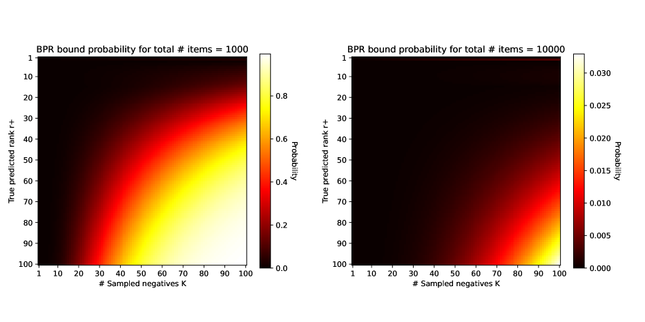
(a) BPR bound probabilities

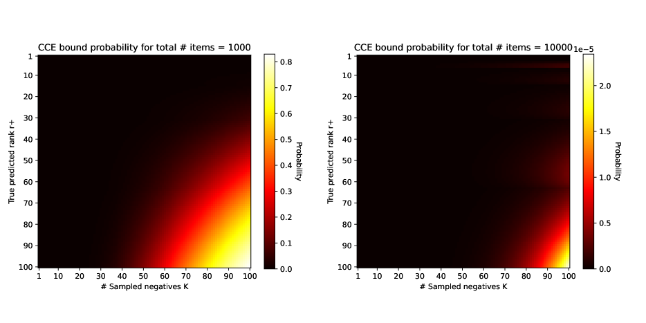
(b) CCE bound probabilities

Figure 5: BPR and CCE bound probabilities as a function of the number of sampled negatives $K$ and the predicted rank $r_{+}$.

Appendix F Reciprocal Rank

The following theorems state that the $\ell_{BPR}$, $\ell_{BCE}$, and $\ell_{gBCE}$ losses are soft-proxy to the RR, i.e. minimizing these losses is equivalent to maximizing a lower bound of the RR.

Theorem 7.

Let consider the BPR loss when, for each user, we uniformly sample $K$ negative items for training. Let $\Gamma=\{i\in I^{-}:s_{i}\geq s_{+}\}$ be the set of all negative items that have a score greater or equal to the score of the positive item that is ranked $r_{+}$. Then we have

$$-log(RR(r_{+}))\leq\ell_{BPR}$$ (20)

with probability at least

$$1-\sum_{i=0}^{\log_{2}(r_{+})}\frac{\binom{|\Gamma|}{i}\binom{|\mathcal{I^{-}}|-|\Gamma|}{K-i}}{\binom{|\mathcal{I^{-}}|}{K}}$$ (21)

Proof.

According to Lemma 3 we know that

$$\ell_{BPR}\geq|\Gamma^{K}|\log 2$$

Therefore, Eq. 20 can be rewritten as follows:

$$P(-\log\text{RR}(r_{+})\leq\ell_{BPR}) \geq P\left(-\log\left(\frac{1}{r_{+}}\right)\leq|\Gamma^{K}|\log 2\right)$$ (22)

$$=P\left(r^{+}\leq 2^{|\Gamma^{K}|}\right) =P\left(|\Gamma^{K}|\geq\log_{2}(r_{+})\right)$$

According to Lemma 2 of the main paper, the $|\Gamma^{K}|$ is an hypergeometric variable with population size $|\mathcal{I^{-}}|$, $|\Gamma^{K}|$ number of successes and $K$ number of draws. Thus, we can rewrite LABEL:eq:prob_BPR_RR using the cumulative distribution function of an hypergeometric:

$$P\left(|\Gamma^{K}|\geq\log_{2}(r_{+})\right)=1-CDF_{|\Gamma^{K}|}\left(\log_{2}(r_{+})\right)$$

that is

$$P\left(-log(RR(r_{+}))\leq\ell_{BPR}\right)\geq\left(1-\sum_{i=0}^{\log_{2}(r_{+})}\frac{\binom{|\Gamma|}{i}\binom{|\mathcal{I^{-}}|-|\Gamma|}{K-i}}{\binom{|\mathcal{I^{-}}|}{K}}\right)$$

∎

Theorem 8.

Let consider the BCE loss when, for each user, we uniformly sample $K$ negative items for training. Let $\Gamma_{0}=\{i\in I^{-}:s_{i}\geq 0\}$ be the set of all negative items that have a non-negative score. Then we have

$$-log(RR(r_{+}))\leq\ell_{BCE}$$ (24)

with probability at least

$$1-\sum_{i=0}^{\log_{2}(r_{+})}\frac{\binom{|\Gamma_{0}|}{i}\binom{|\mathcal{I^{-}}|-|\Gamma^{0}|}{K-i}}{\binom{|\mathcal{I^{-}}|}{K}}$$ (25)

Proof.

According to Lemma 4 we know that

$$\ell_{BCE}\geq|\Gamma^{K}_{0}|\log 2$$

Thus, the demonstration is equivalent to that of Theorem 4, using the set $\Gamma_{0}^{K}$ instead of $\Gamma^{K}$. ∎

Theorem 9.

Let consider the CCE loss when, for each user, we uniformly sample $K$ negative items for training. Let $\Gamma=\{i\in I^{-}:s_{i}\geq s_{+}\}$ be the set of all negative items that have a score greater or equal to the score of the positive item that is ranked $r_{+}$. Then we have

$$-log(RR(r_{+}))\leq\ell_{CCE}$$ (26)

with probability at least

$$1-\sum_{i=0}^{r_{+}}\frac{\binom{|\Gamma|}{i}\binom{|\mathcal{I^{-}}|-|\Gamma|}{K-i}}{\binom{|\mathcal{I^{-}}|}{K}}$$ (27)

Proof.

According to Lemma 5 we know that

$$\ell_{BPR}\geq\log(|\Gamma^{K}|)$$

Therefore, Eq. 16 can be rewritten as follows:

$$P(-\log\text{RR}(r_{+})\leq\ell_{CCE}) \geq P\left(-\log\left(\frac{1}{r_{+}}\right)\leq\log(|\Gamma^{K}|)\right)$$ (28)

$$=P\left(|\Gamma^{K}|\geq r_{+}\right)$$

According to Lemma 2 of the main paper, the set $\Gamma^{K}$ is an hypergeometric variable with population size $|\mathcal{I^{-}}|$, $|\Gamma^{K}|$ number of successes and $K$ number of draws. Thus, we can rewrite LABEL:eq:prob_BPR using the cumulative distribution function of an hypergeometric:

$$P\left(|\Gamma^{K}|\geq r_{+}\right)=1-CDF_{|\Gamma^{K}|}\left(r_{+}\right)$$

that is

$$P\left(-log(RR(r_{+}))\leq\ell_{CCE}\right)\geq\left(1-\sum_{i=0}^{r_{+}}\frac{\binom{|\Gamma|}{i}\binom{|\mathcal{I^{-}}|-|\Gamma|}{K-i}}{\binom{|\mathcal{I^{-}}|}{K}}\right)$$

∎

Appendix G Results

Hardware All experiments were performed on a workstation equipped with an Intel Core i9-10940X (14-core CPU running at 3.3GHz) and 256GB of RAM, and a single Nvidia RTX A6000 with 48GB of VRAM.

Additional datasets. To ensure the generalizability of our results, we incorporated two larger real-world benchmark datasets for RSs:

• Amazon Books (McAuley et al.,, 2015): This dataset contains user reviews and ratings specifically for books available on Amazon. It includes detailed information on user interactions, allowing for a nuanced analysis of preferences and behaviors across a wide selection of book titles. It encompasses reviews from 52,643 users on 91,599 items, totalling 2,984,108 interactions.

• Yelp (http://www.yelp.com/dataset_challenge): This dataset consists of user reviews, ratings, and business information from Yelp, covering a diverse range of categories such as restaurants, nightlife, and shopping. It captures user interactions within the local business landscape, providing insights into user preferences in various service sectors. It encompasses reviews from 31,668 users on 38,048 items, totalling 1,561,406 interactions.

Additional baselines. To ensure a comprehensive evaluation, we include two prominent, state-of-the-art non-sequential RSs:

• (i) NCF (He et al.,, 2017) that utilizes a neural collaborative filtering approach to model user-item interactions;

• (ii) LightGCN (He et al.,, 2020) that employs a simplified graph convolutional network designed specifically for recommendation tasks.

Table 1: NDCG@10 for all the configuration considered, training the models for 600 epochs. Best results for each model are highlighted in bold. $\dagger$ indicates a statistically significant result at level 0.01 using a Mann–Whitney–Wilcoxon test.

		GRU4Rec			SASRec
Dataset	Negative items	BCE	BPR	CCE	BCE	BPR	CCE
Beauty	1	0.6848	0.6836	0.6788	0.6304	0.6723	0.6758†
Beauty	5	0.6806	0.6843†	0.6784	0.5719	0.6753	0.6783
Beauty	10	0.6822	0.6865†	0.6802	0.6776	0.6753	0.6734
Beauty	50	0.6834	0.6848	0.6819	0.5968	0.6702	0.6781†
Beauty	100	0.6808	0.6848	0.6835	0.5070	0.6745	0.6819†
FS-NYC	1	0.6369	0.6369	0.6174	0.6562†	0.6009	0.6107
FS-NYC	5	0.6051	0.6331	0.6484†	0.6713	0.6242	0.6676
FS-NYC	10	0.5887	0.6249	0.6476†	0.6600	0.6288	0.6782†
FS-NYC	50	0.5713	0.6321	0.6513†	0.5973	0.6502	0.6994†
FS-NYC	100	0.4969	0.6332	0.6751†	0.5470	0.6519	0.7150†
ML-1M	1	0.5627	0.5627	0.5611	0.5704	0.5640	0.5640
ML-1M	5	0.5661	0.5692	0.5710	0.5961†	0.5807	0.5955
ML-1M	10	0.5808†	0.5669	0.5694	0.5992†	0.5790	0.5966
ML-1M	50	0.5877	0.5628	0.5834	0.6010	0.5807	0.6060
ML-1M	100	0.5909	0.5604	0.5907	0.5988	0.5822	0.6053

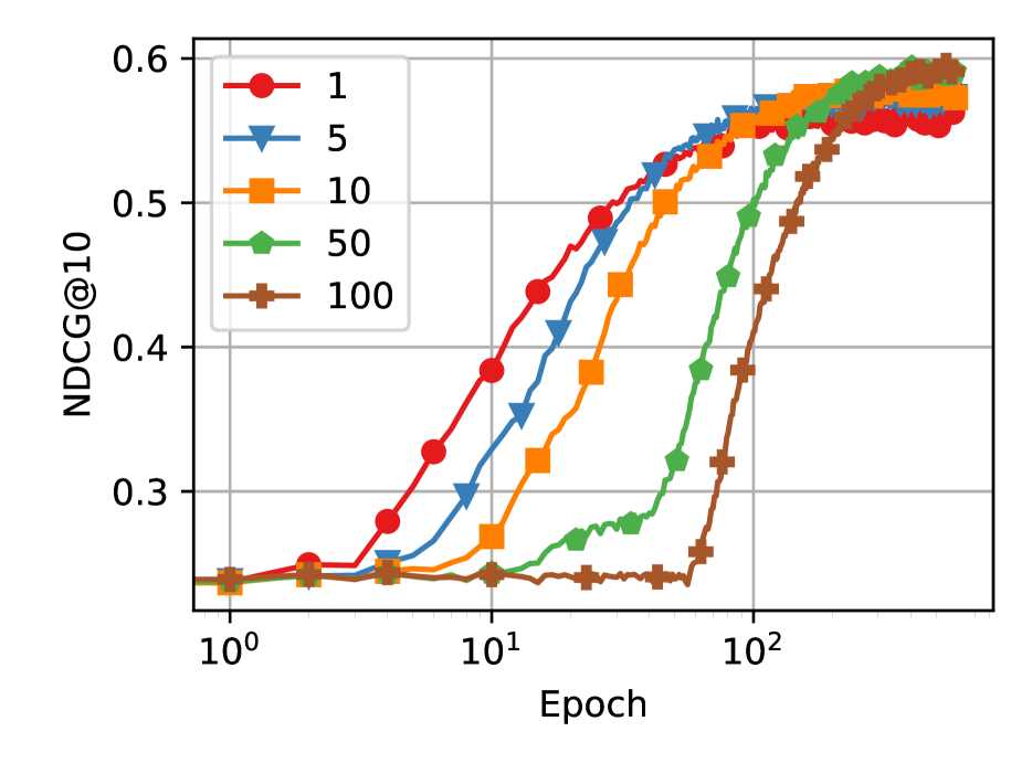
(a) GRU4Rec

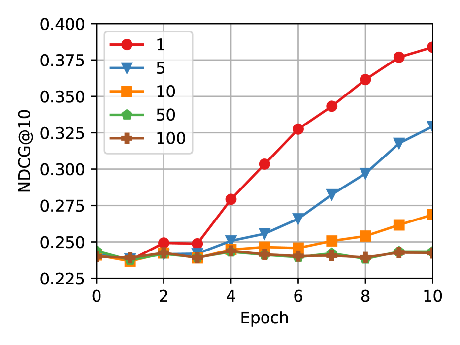
(b) GRU4Rec - Start

(c) GRU4Rec - End

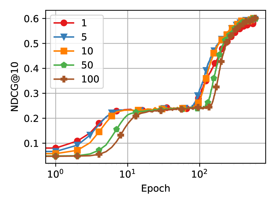
(d) SASRec

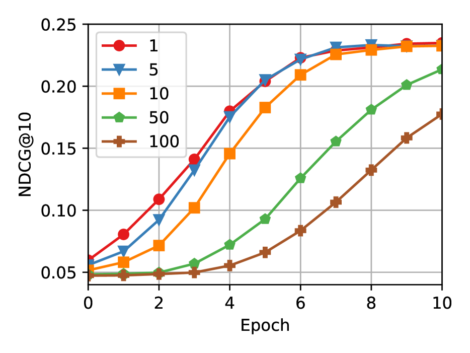
(e) SASRec - Start

(f) SASRec - End

Figure 6: SASRec and GRU4Rec NDCG@10 during training changing number of negative items, using BCE loss on ML-1M dataset.

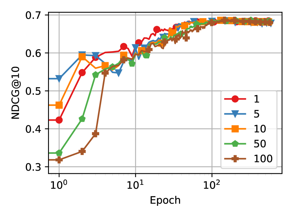
(a) GRU4Rec

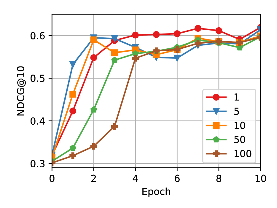
(b) GRU4Rec - Start

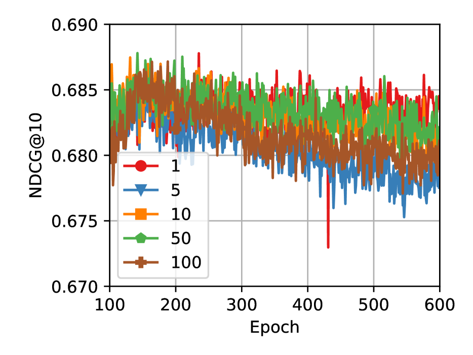
(c) GRU4Rec - End

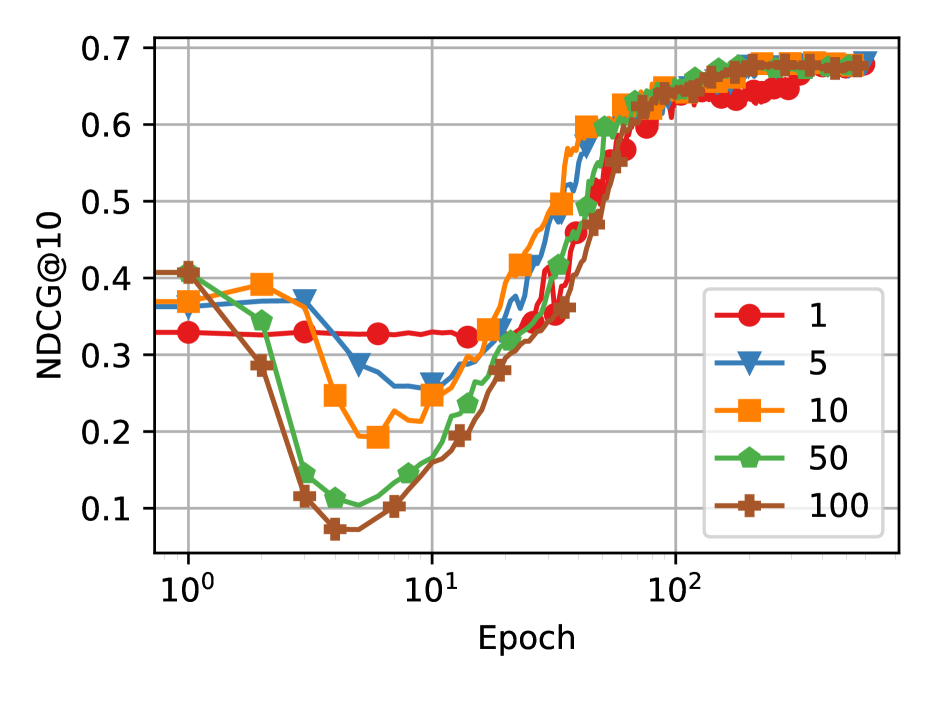
(d) SASRec

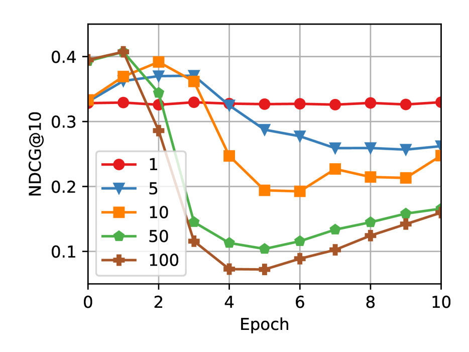
(e) SASRec - Start

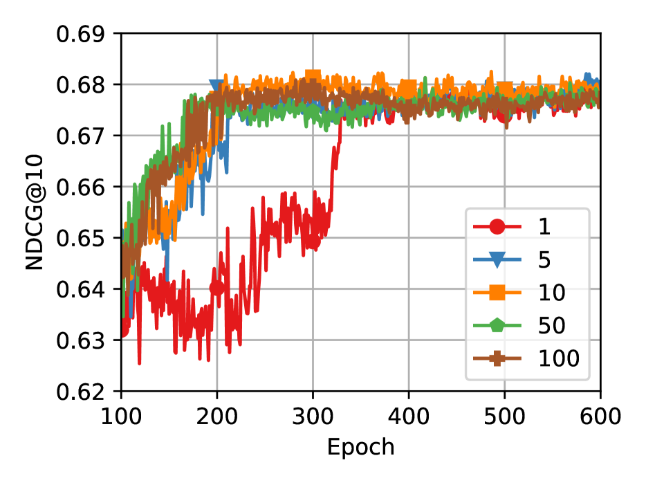
(f) SASRec - End

Figure 7: SASRec and GRU4Rec NDCG@10 during training changing number of negative items, using BCE loss on Amazon Beauty dataset.

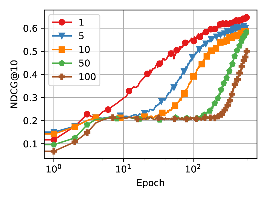
(a) GRU4Rec

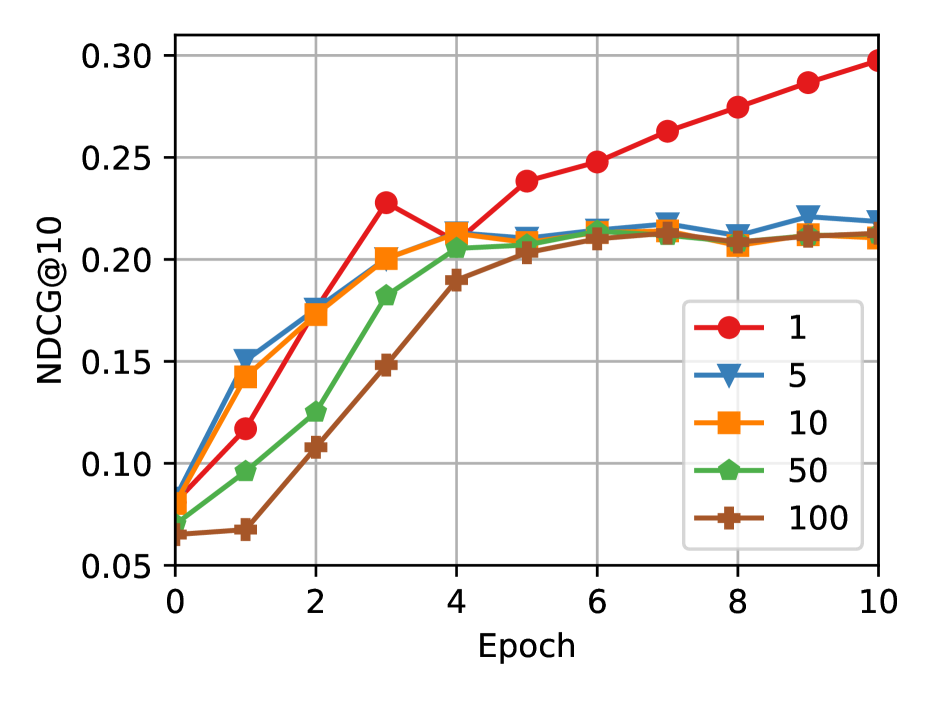
(b) GRU4Rec - Start

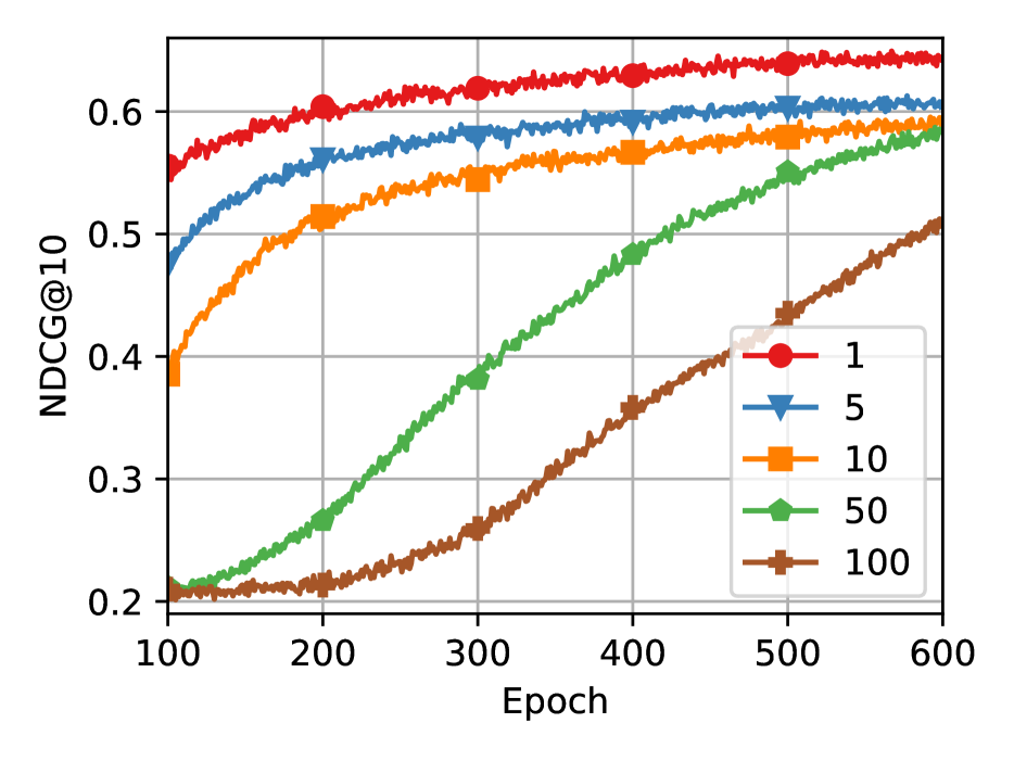
(c) GRU4Rec - End

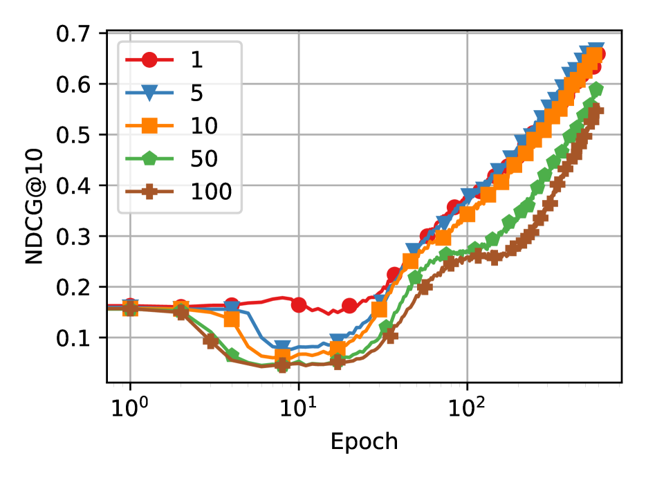
(d) SASRec

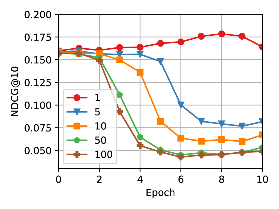
(e) SASRec - Start

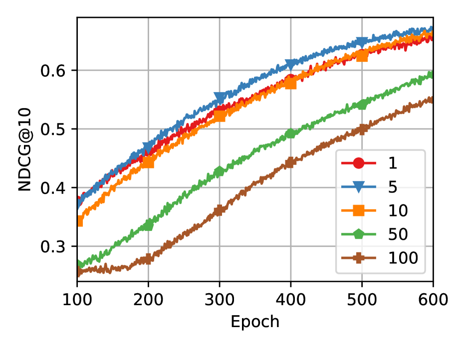
(f) SASRec - End

Figure 8: SASRec and GRU4Rec NDCG@10 during training changing number of negative items, using BCE loss on Foursquare-NYC dataset.

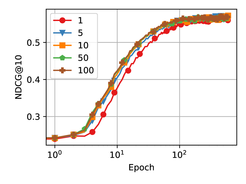
(a) GRU4Rec

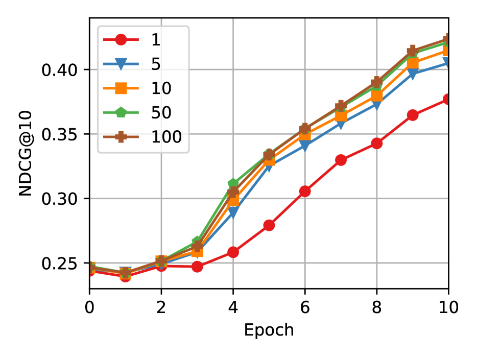
(b) GRU4Rec - Start

(c) GRU4Rec - End

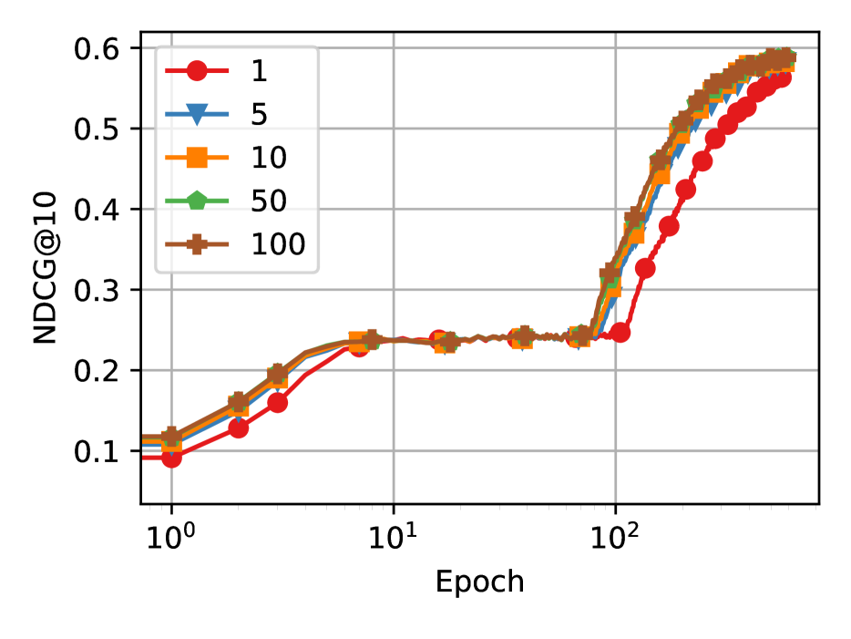
(d) SASRec

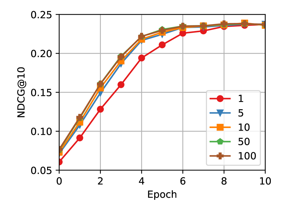
(e) SASRec - Start

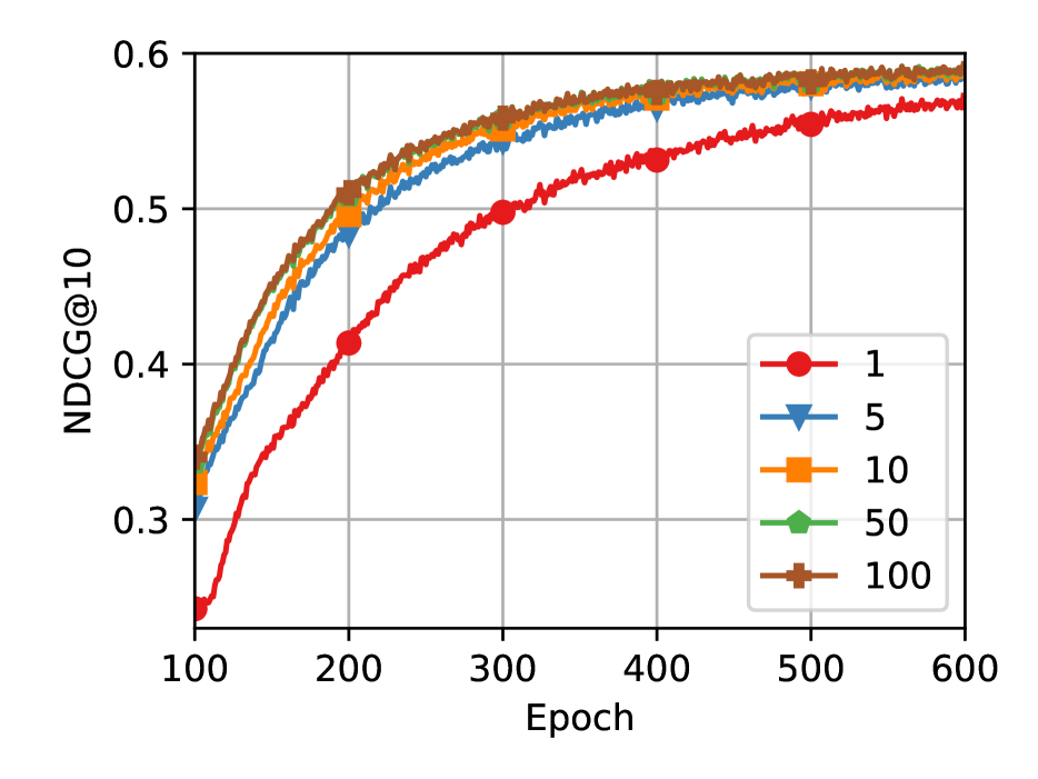
(f) SASRec - End

Figure 9: SASRec and GRU4Rec NDCG@10 during training changing number of negative items, using BPR loss on ML-1M dataset.

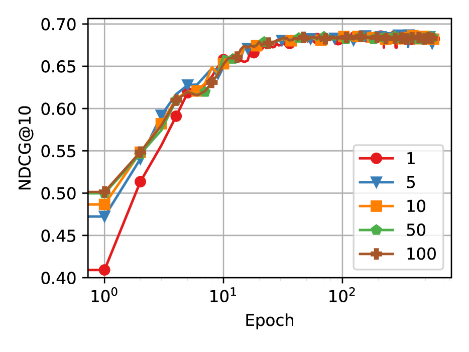
(a) GRU4Rec

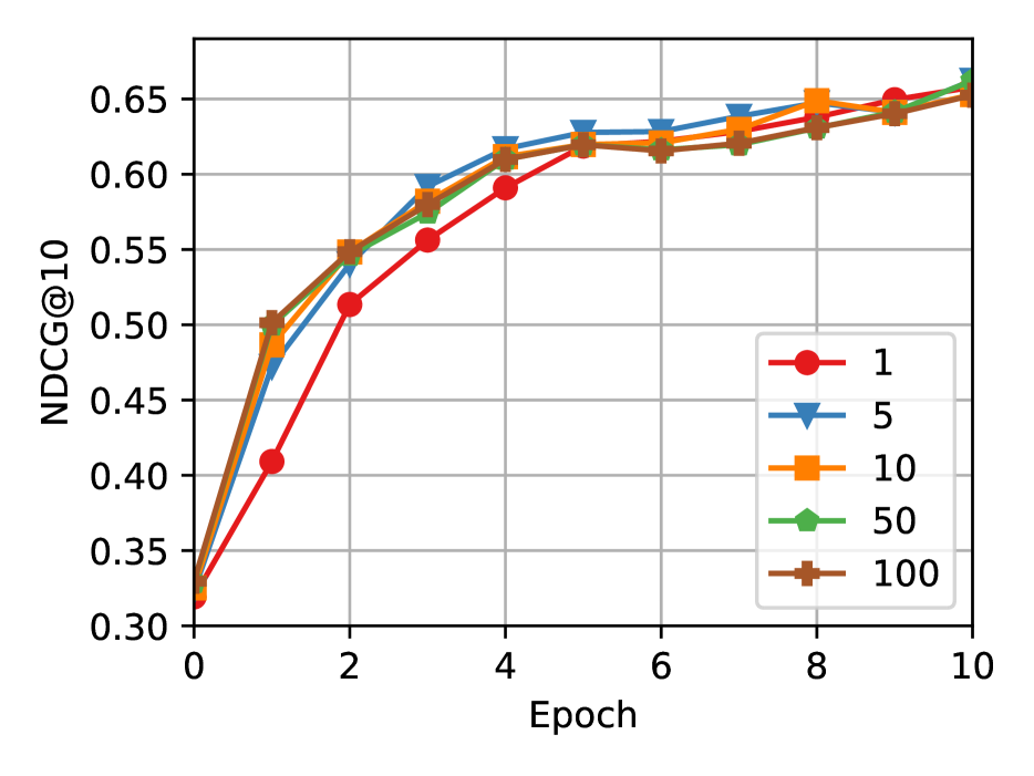
(b) GRU4Rec - Start

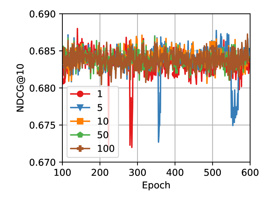
(c) GRU4Rec - End

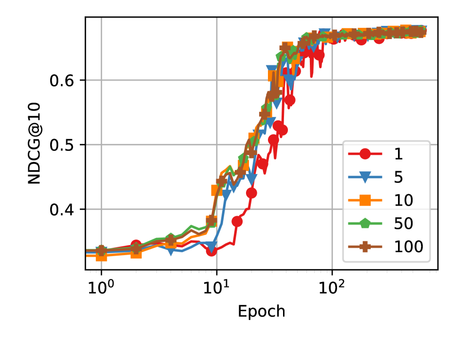
(d) SASRec

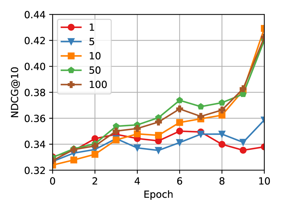
(e) SASRec - Start

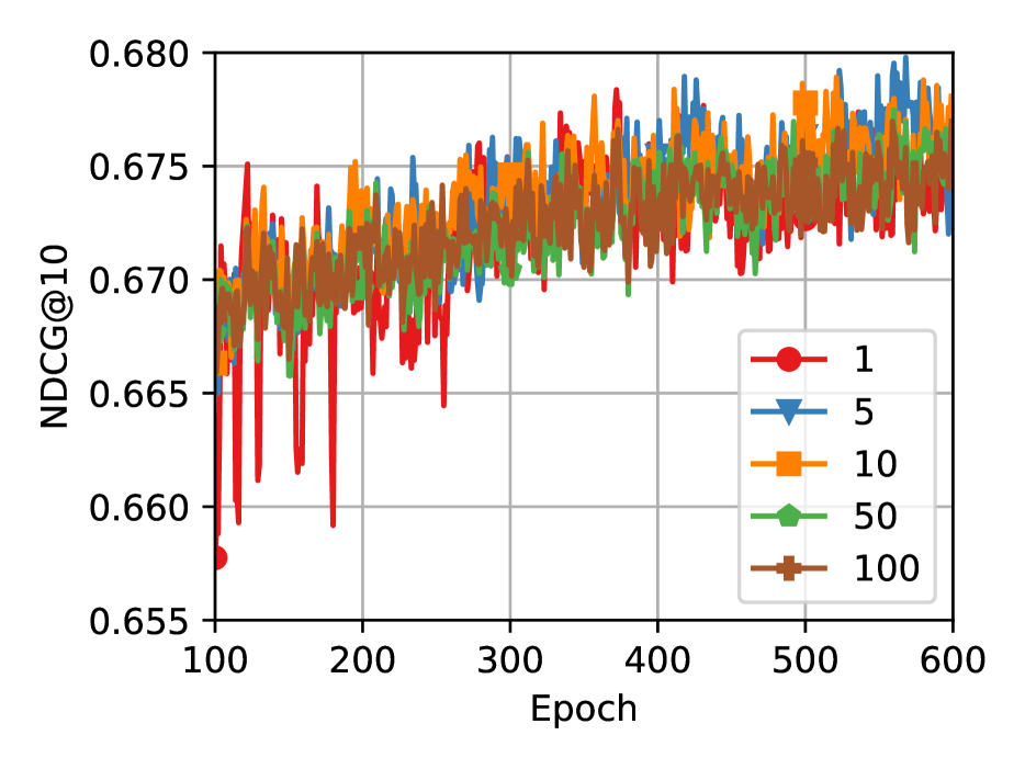
(f) SASRec - End

Figure 10: SASRec and GRU4Rec NDCG@10 during training changing number of negative items, using BPR loss on Amazon Beauty dataset.

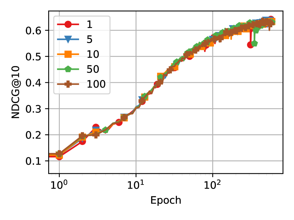
(a) GRU4Rec

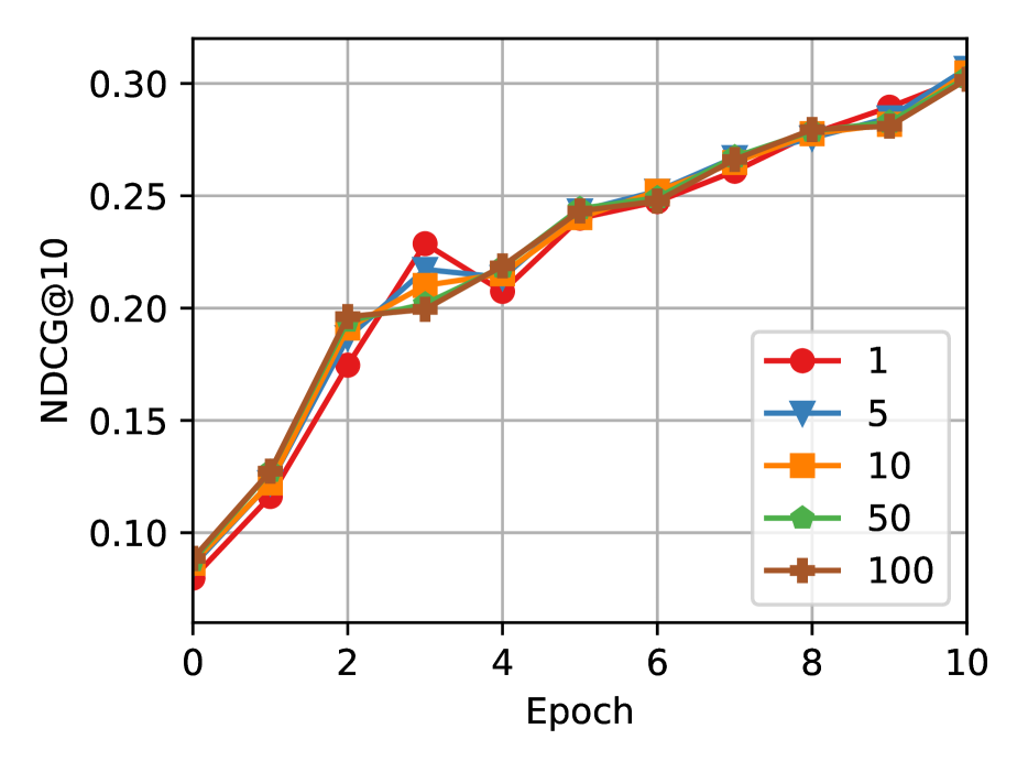
(b) GRU4Rec - Start

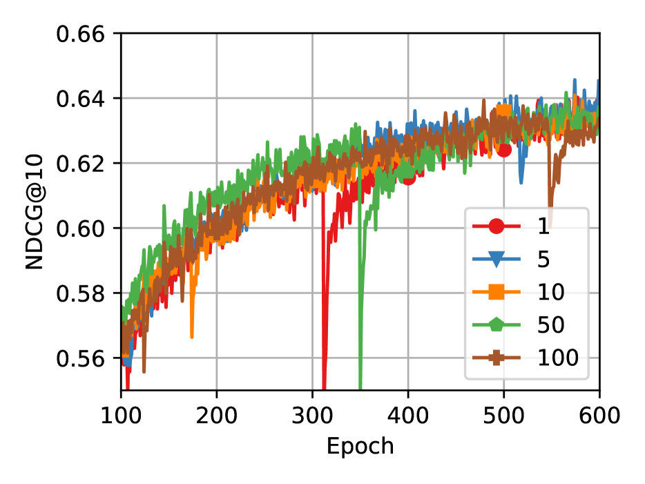
(c) GRU4Rec - End

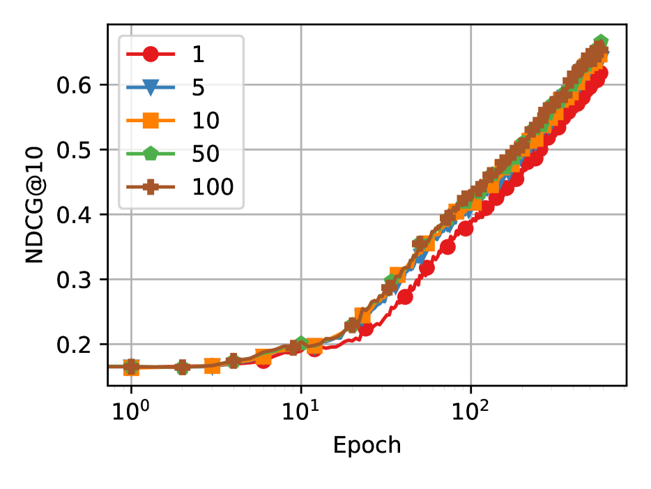
(d) SASRec

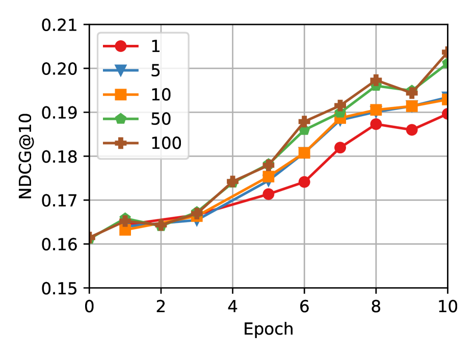
(e) SASRec - Start

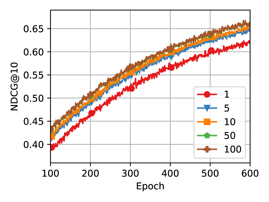
(f) SASRec - End

Figure 11: SASRec and GRU4Rec NDCG@10 during training changing number of negative items, using BPR loss on Foursquare-NYC dataset.

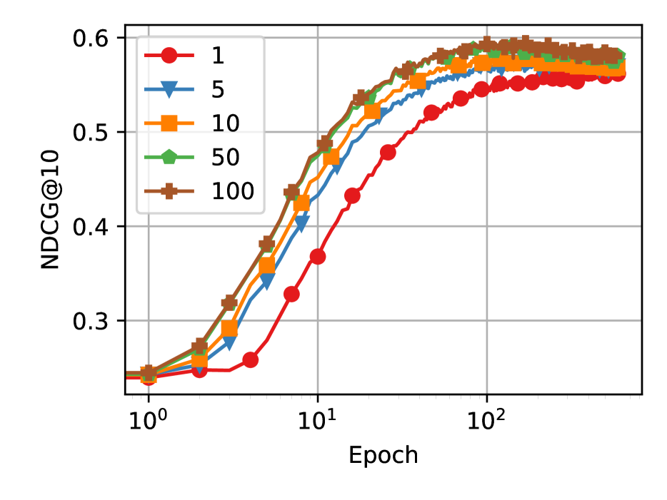
(a) GRU4Rec

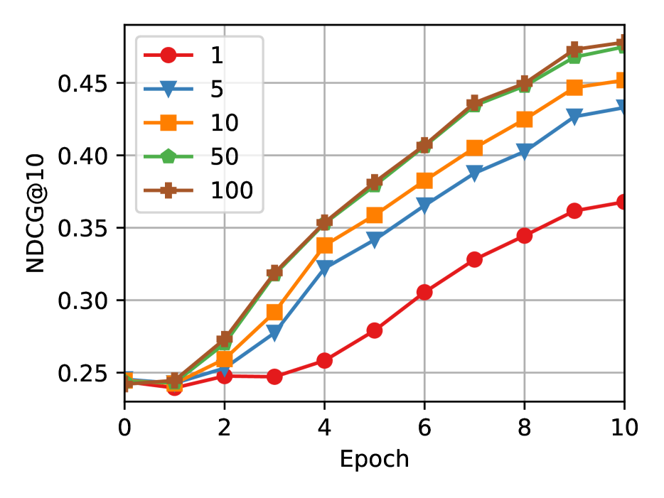
(b) GRU4Rec - Start

(c) GRU4Rec - End

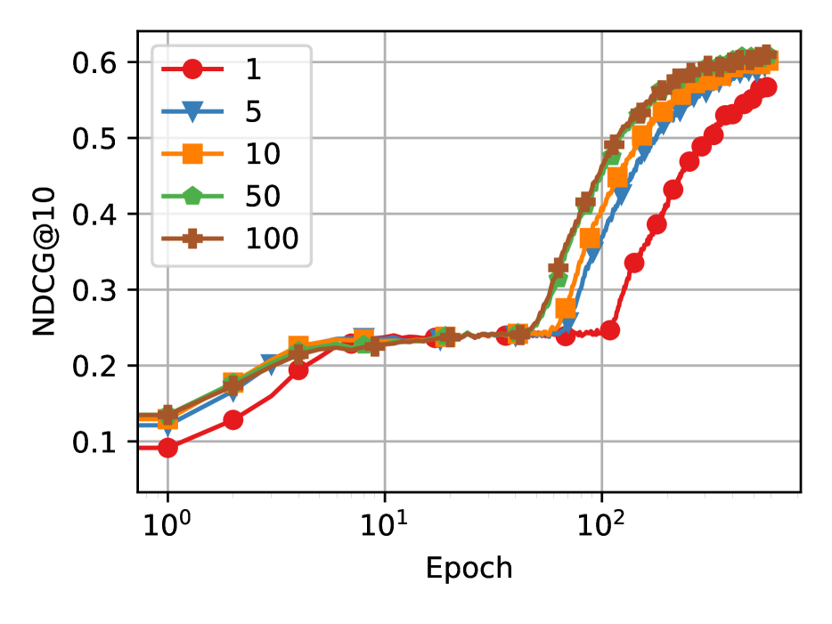
(d) SASRec

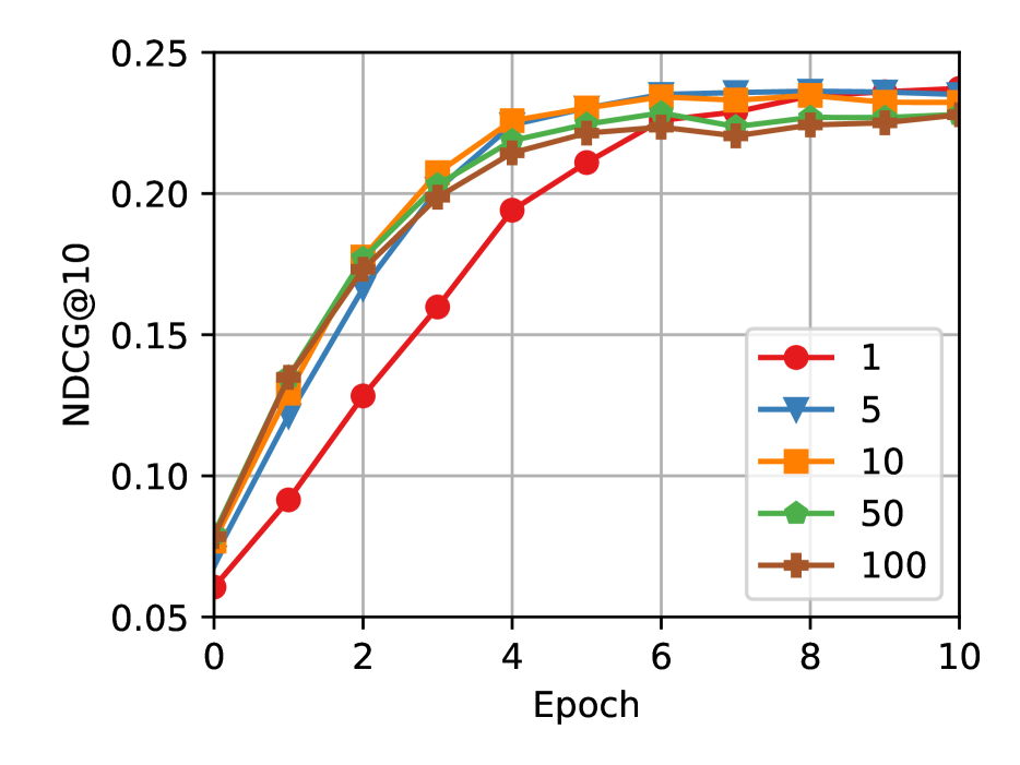
(e) SASRec - Start

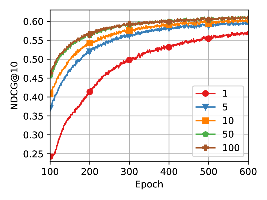
(f) SASRec - End

Figure 12: SASRec and GRU4Rec NDCG@10 during training changing number of negative items, using CCE loss on ML-1M dataset.

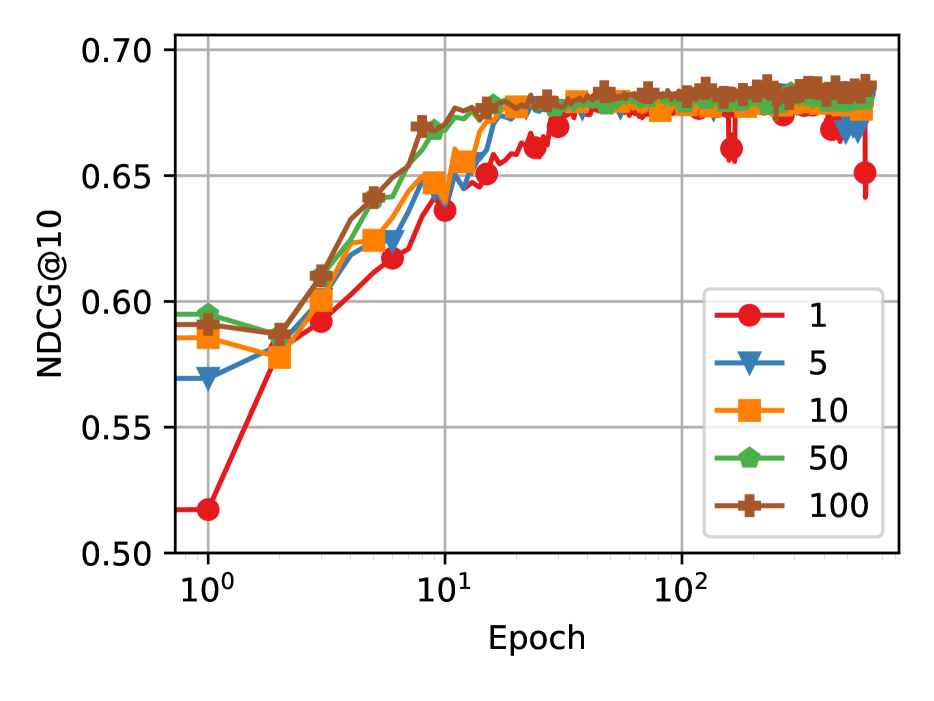
(a) GRU4Rec

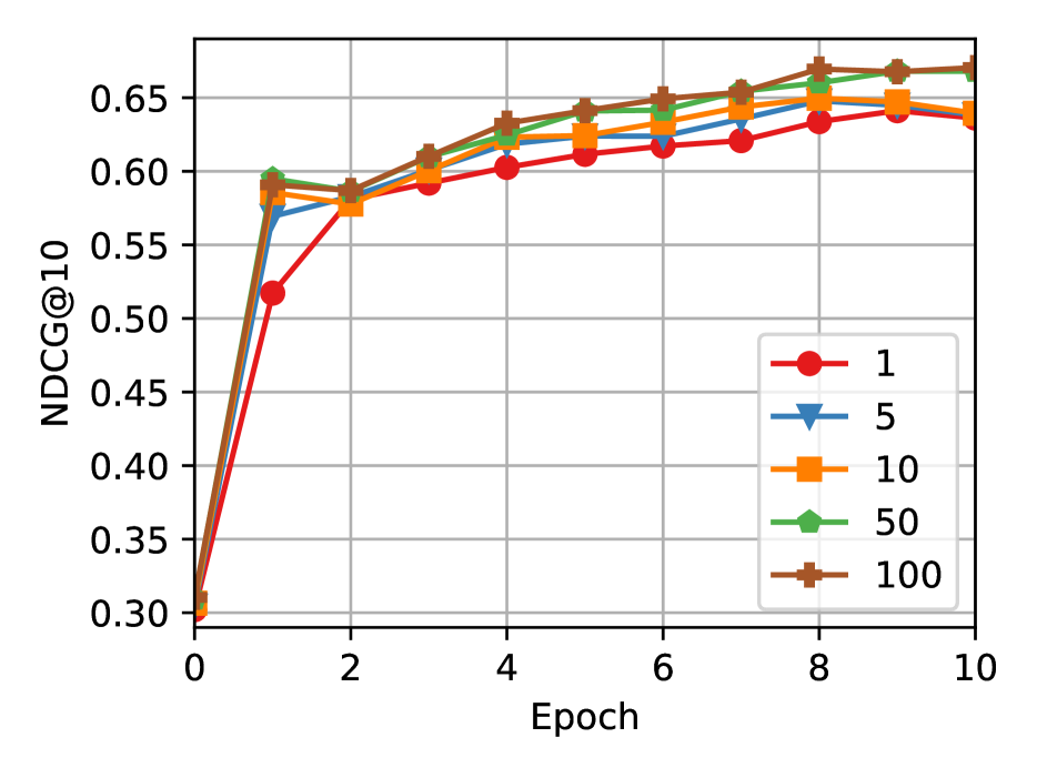
(b) GRU4Rec - Start

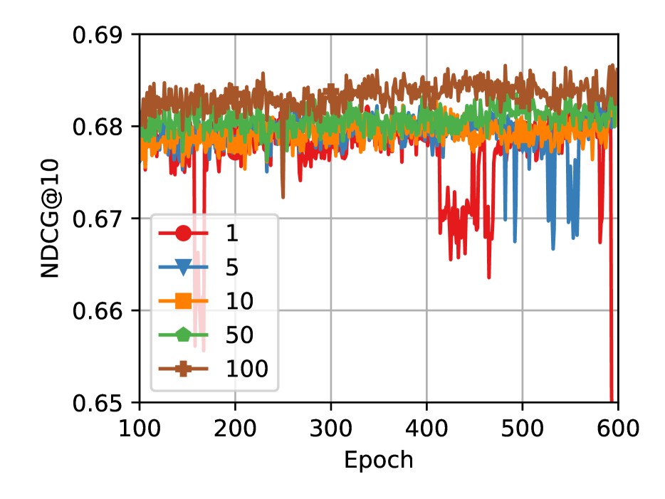
(c) GRU4Rec - End

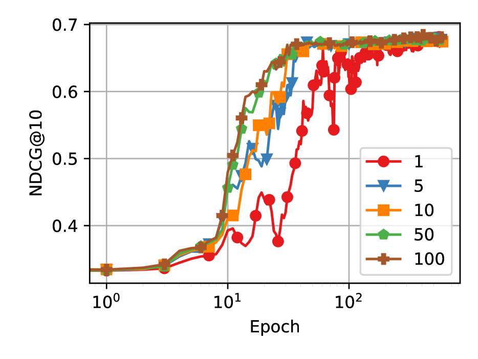
(d) SASRec

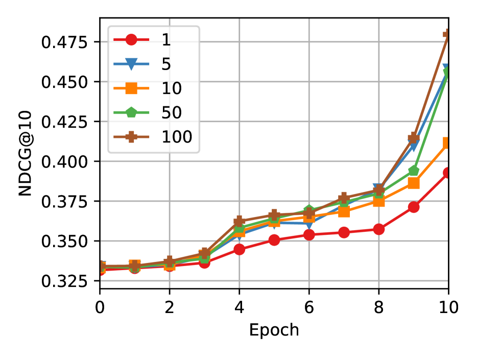
(e) SASRec - Start

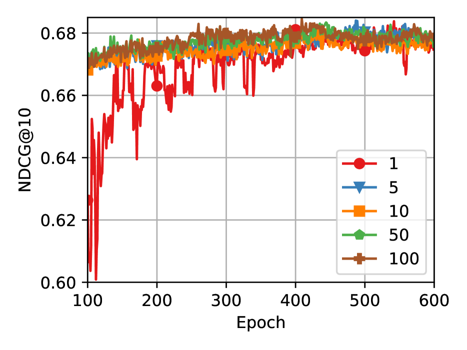
(f) SASRec - End

Figure 13: SASRec and GRU4Rec NDCG@10 during training changing number of negative items, using CCE loss on Amazon Beauty dataset.

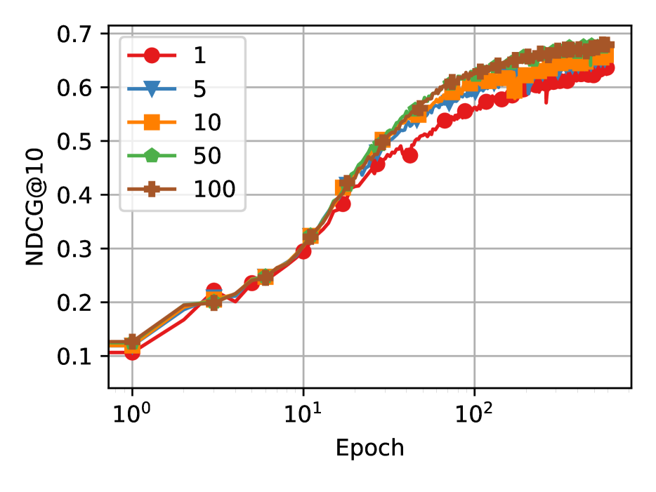
(a) GRU4Rec

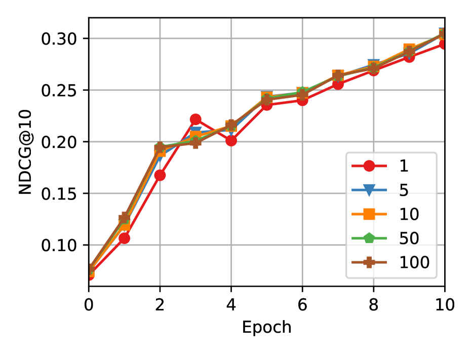
(b) GRU4Rec - Start

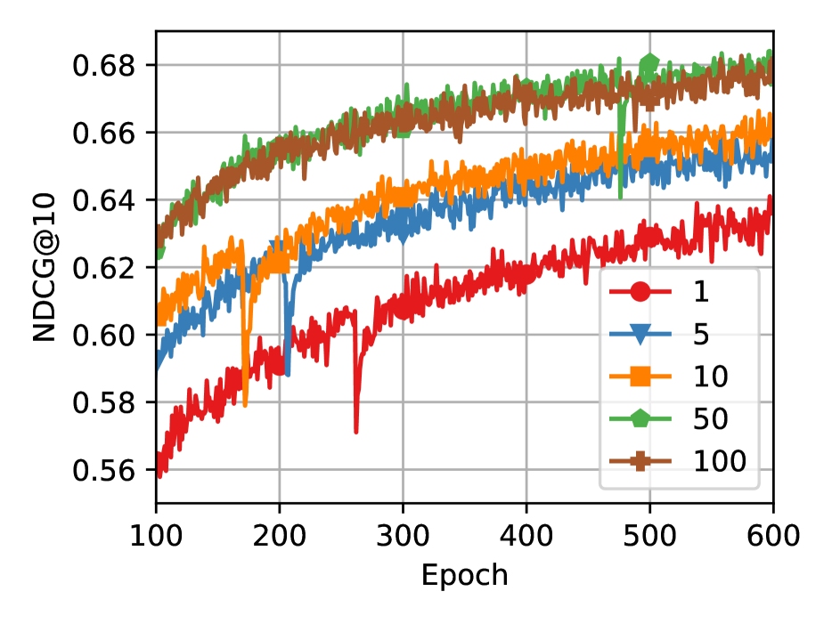
(c) GRU4Rec - End

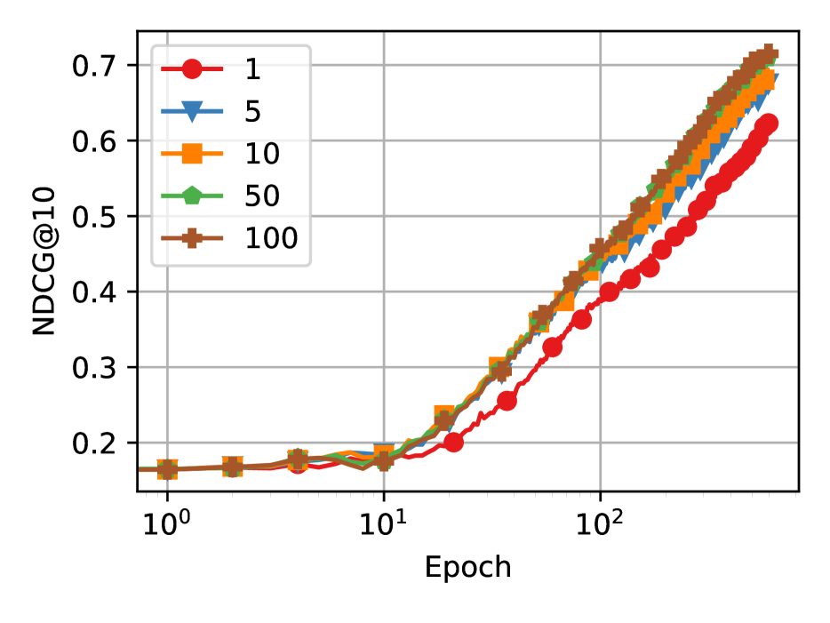
(d) SASRec

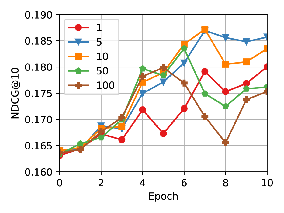
(e) SASRec - Start

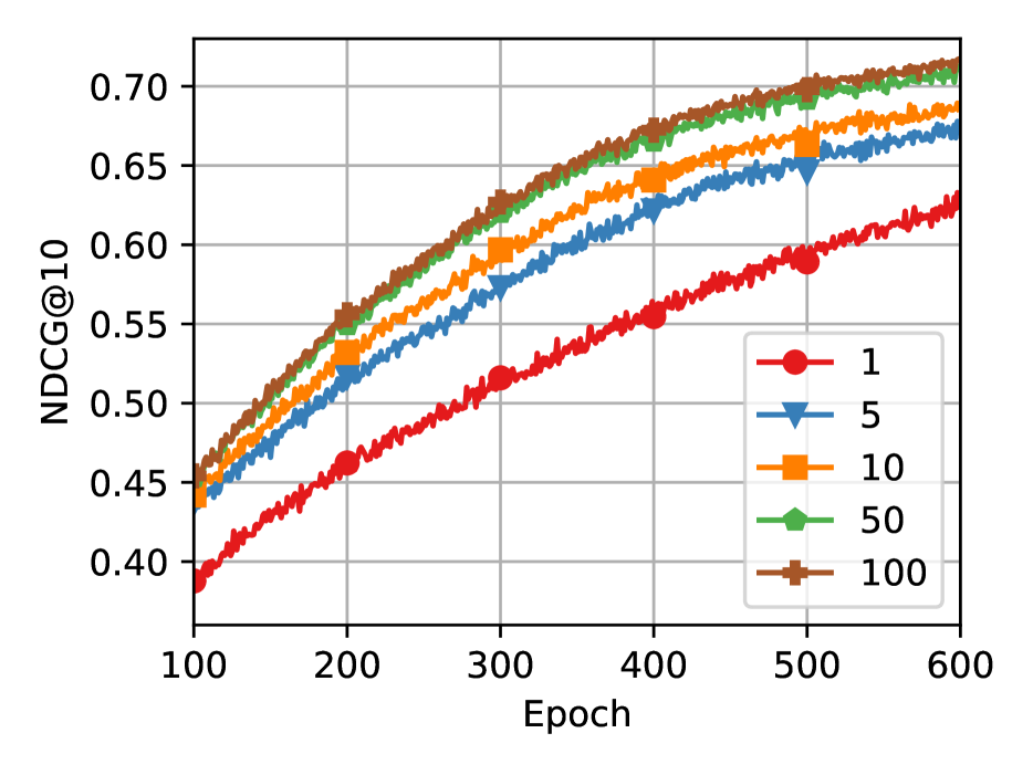
(f) SASRec - End

Figure 14: SASRec and GRU4Rec NDCG@10 during training changing number of negative items, using CCE loss on Foursquare-NYC dataset.

(a) GRU4Rec

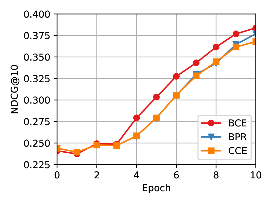
(b) GRU4Rec - Start

(c) GRU4Rec - End

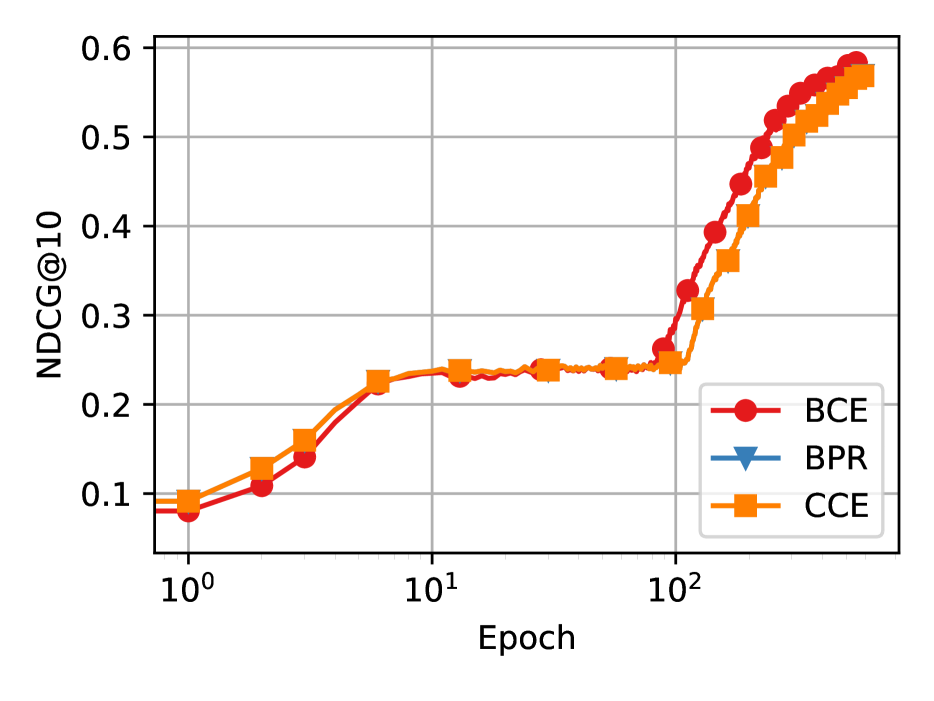
(d) SASRec

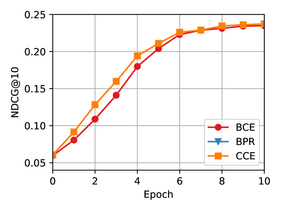
(e) SASRec - Start

(f) SASRec - End

Figure 15: SASRec and GRU4Rec NDCG@10 during training changing loss, using 1 negative item on ML-1M dataset.

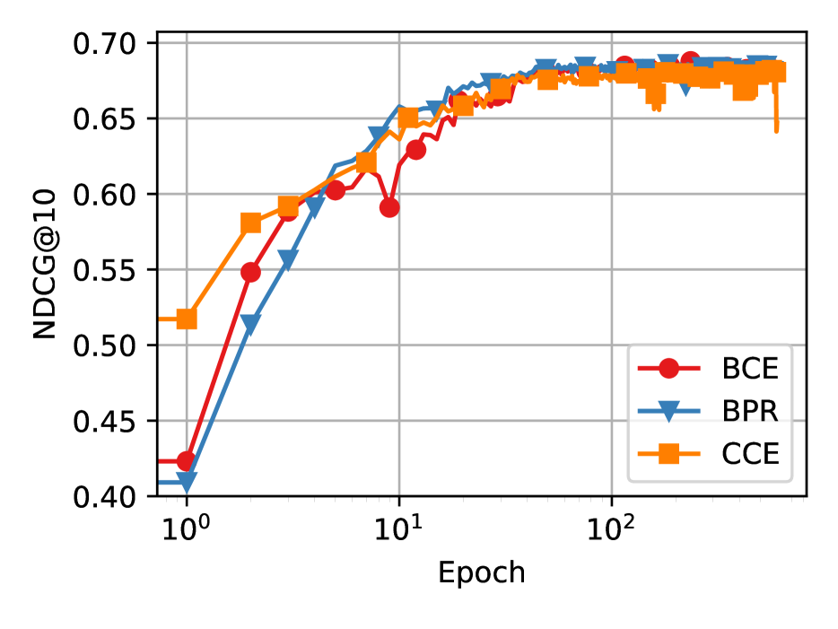
(a) GRU4Rec

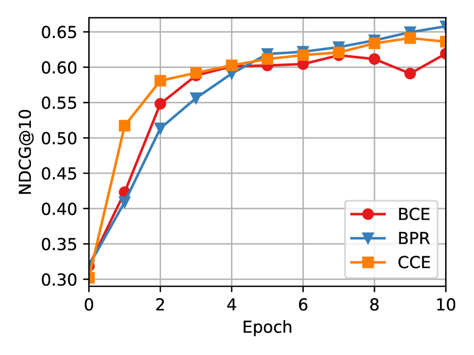
(b) GRU4Rec - Start

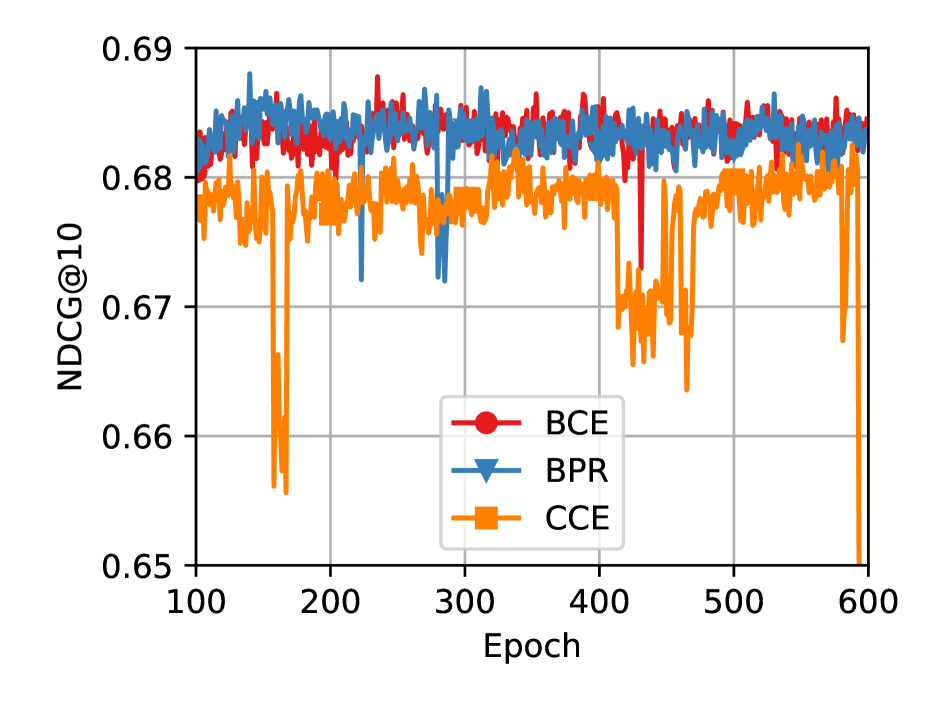
(c) GRU4Rec - End

(d) SASRec

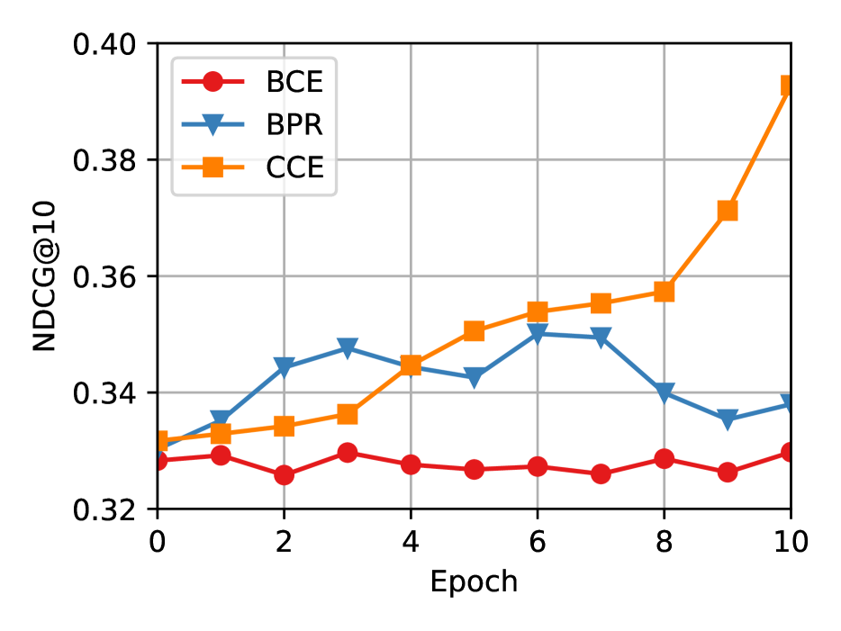
(e) SASRec - Start

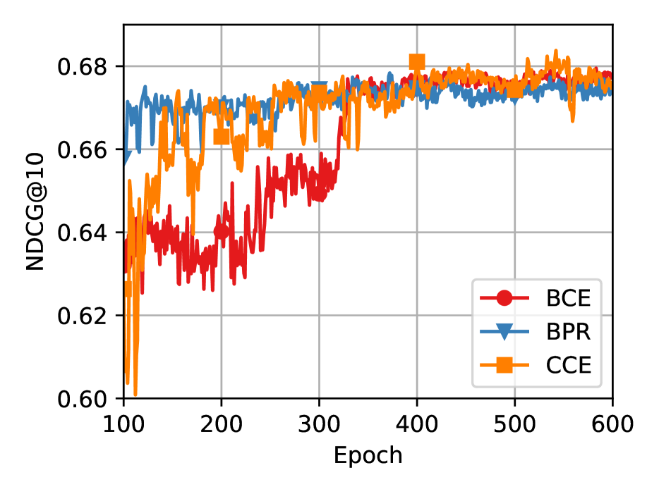
(f) SASRec - End

Figure 16: SASRec and GRU4Rec NDCG@10 during training changing loss, using 1 negative item on Amazon Beauty dataset.

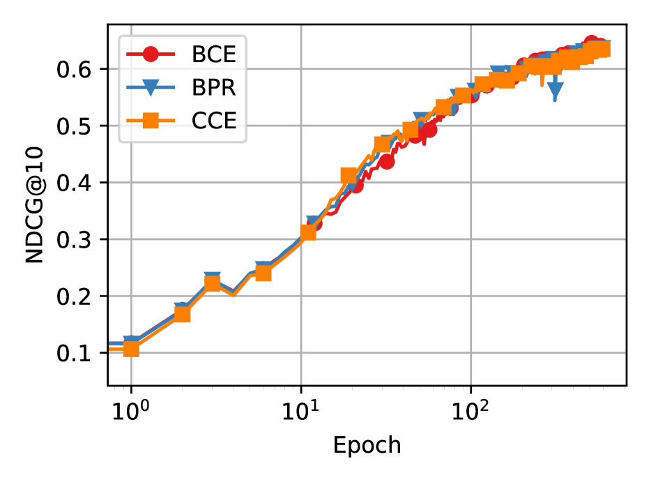
(a) GRU4Rec

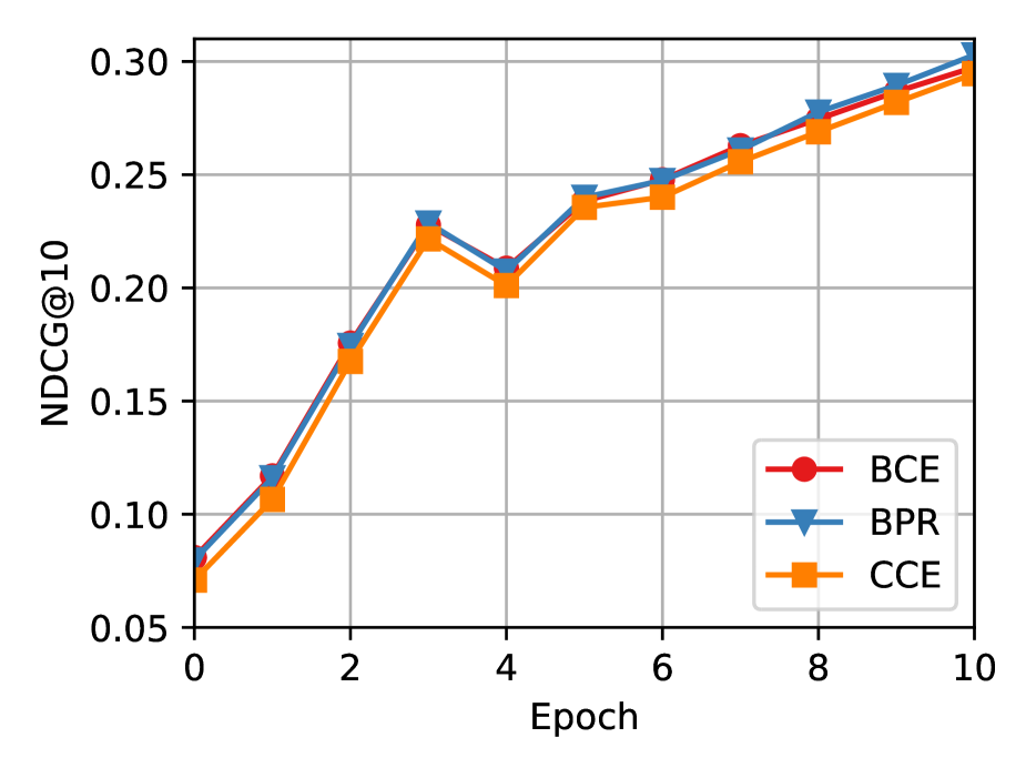
(b) GRU4Rec - Start

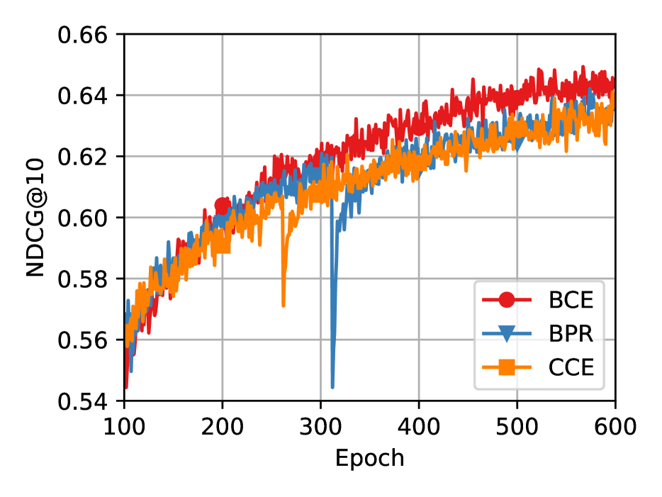
(c) GRU4Rec - End

(d) SASRec

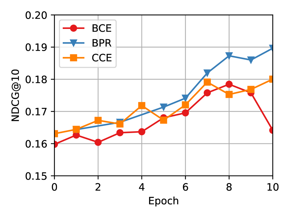
(e) SASRec - Start

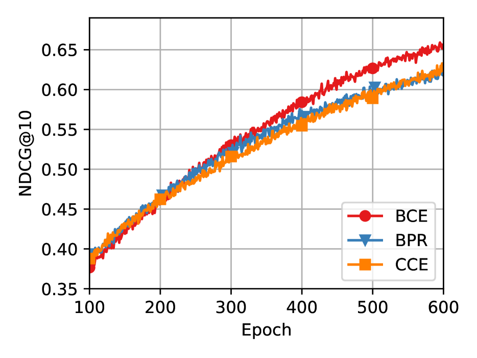
(f) SASRec - End

Figure 17: SASRec and GRU4Rec NDCG@10 during training changing loss, using 1 negative item on Foursquare-NYC dataset.

(a) GRU4Rec

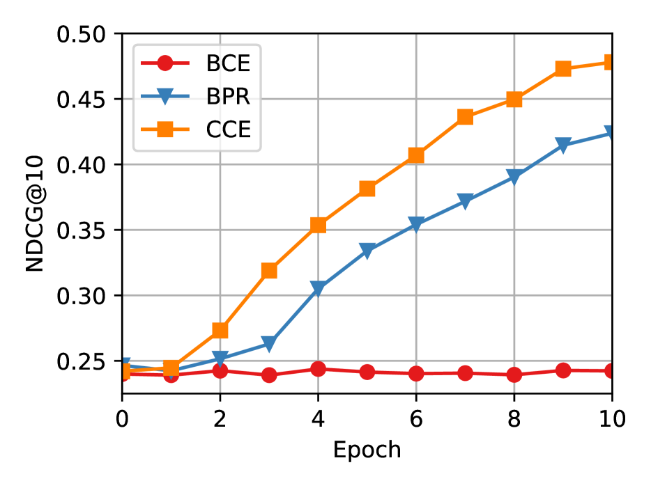
(b) GRU4Rec - Start

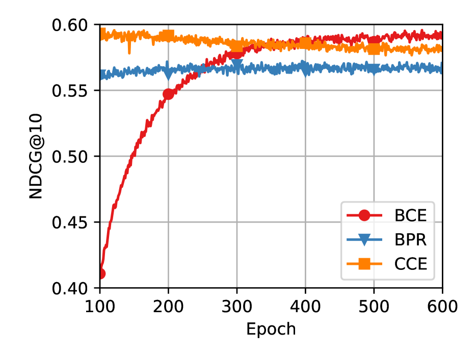
(c) GRU4Rec - End

(d) SASRec

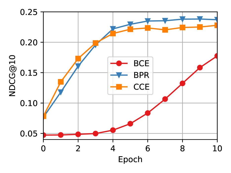
(e) SASRec - Start

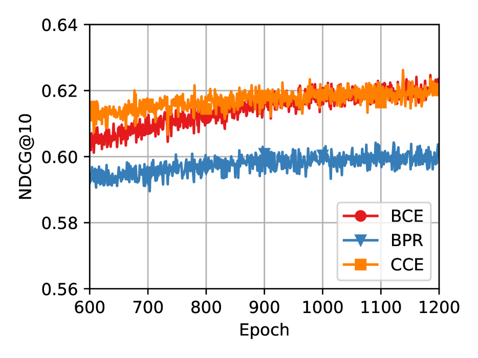
(f) SASRec - End

Figure 18: SASRec and GRU4Rec NDCG@10 during training changing loss, using 100 negative items on ML-1M dataset.

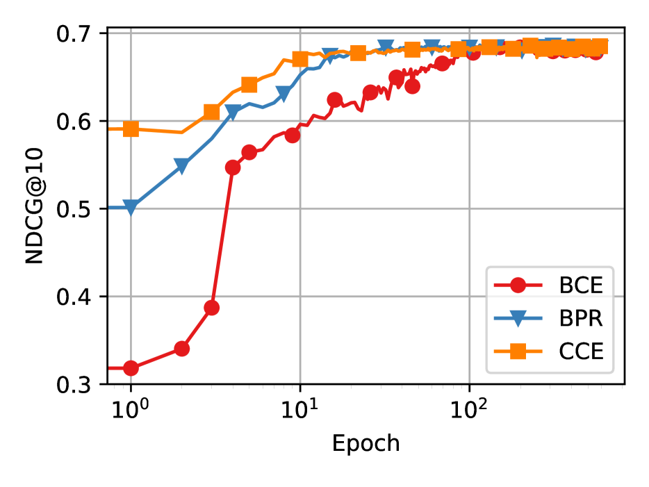
(a) GRU4Rec

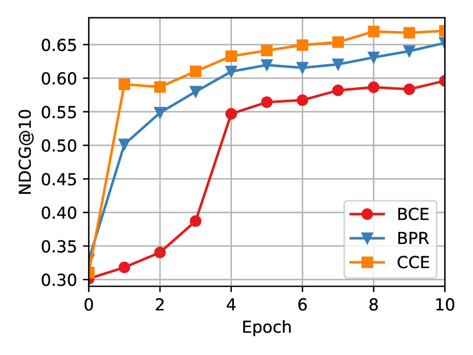
(b) GRU4Rec - Start

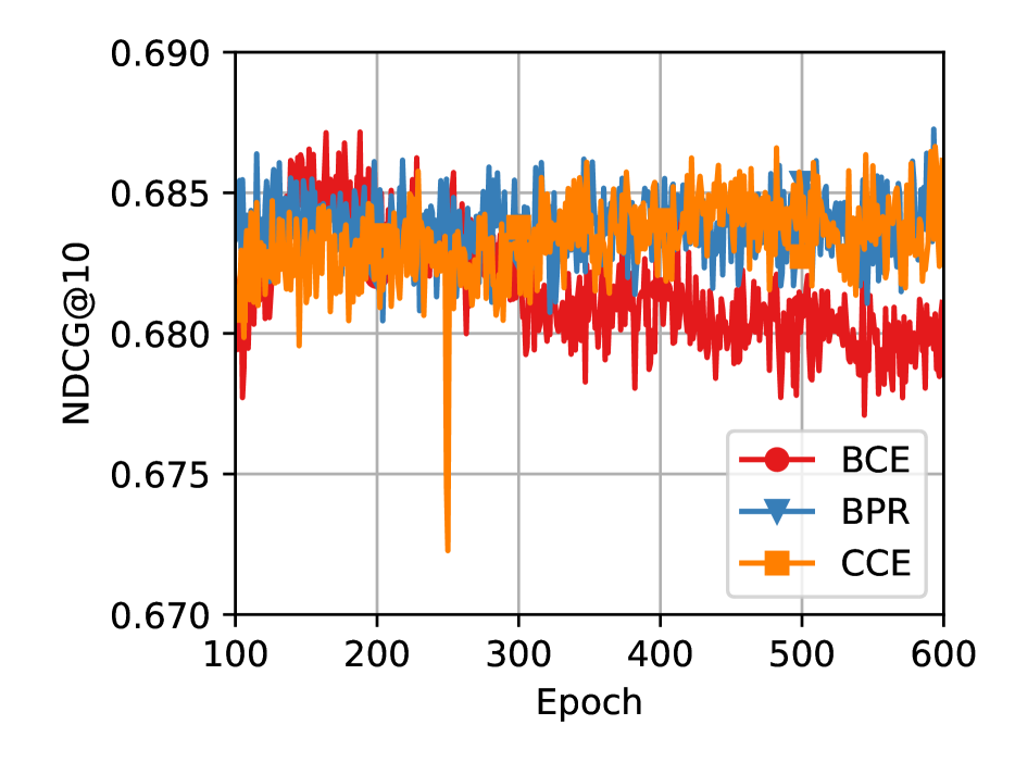
(c) GRU4Rec - End

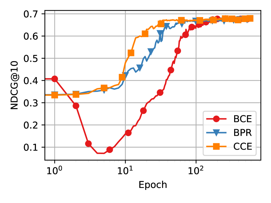
(d) SASRec

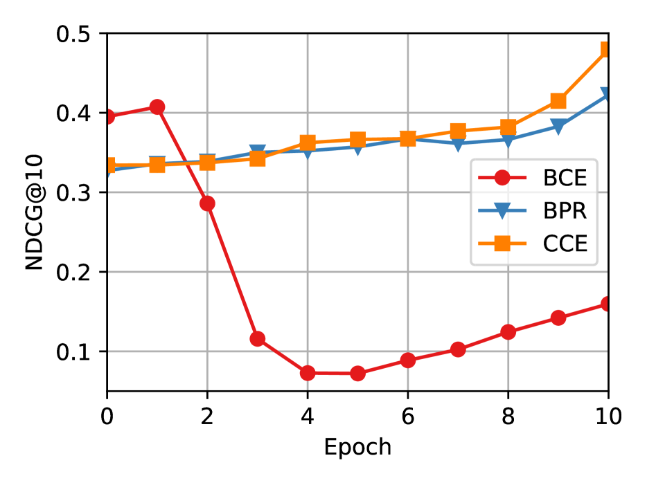
(e) SASRec - Start

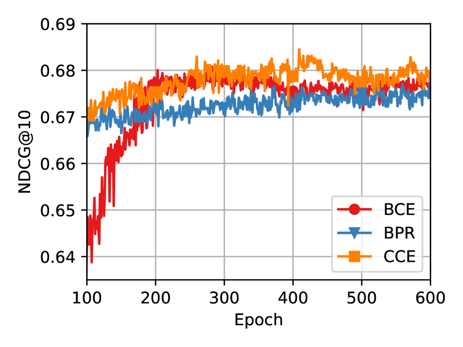
(f) SASRec - End

Figure 19: SASRec and GRU4Rec NDCG@10 during training changing loss, using 100 negative items on Amazon Beauty dataset.

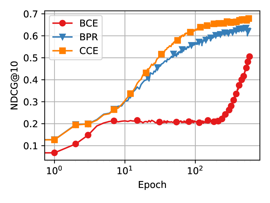
(a) GRU4Rec

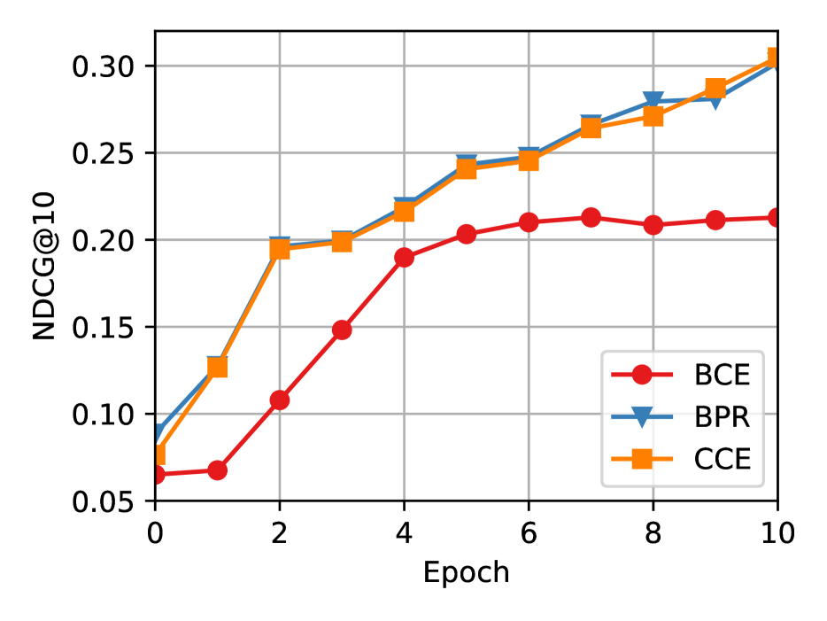
(b) GRU4Rec - Start

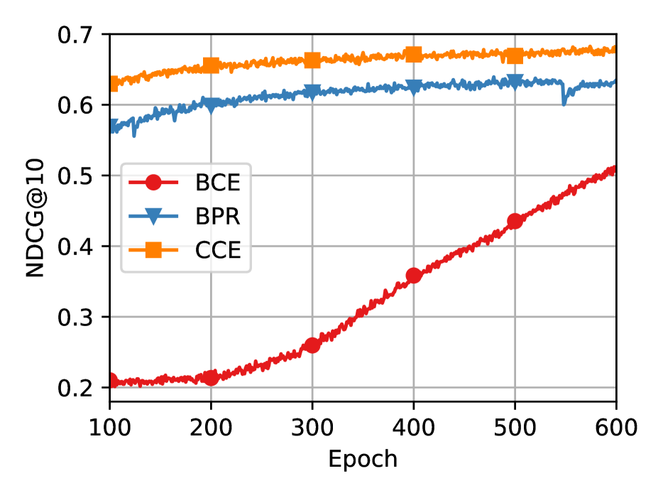
(c) GRU4Rec - End

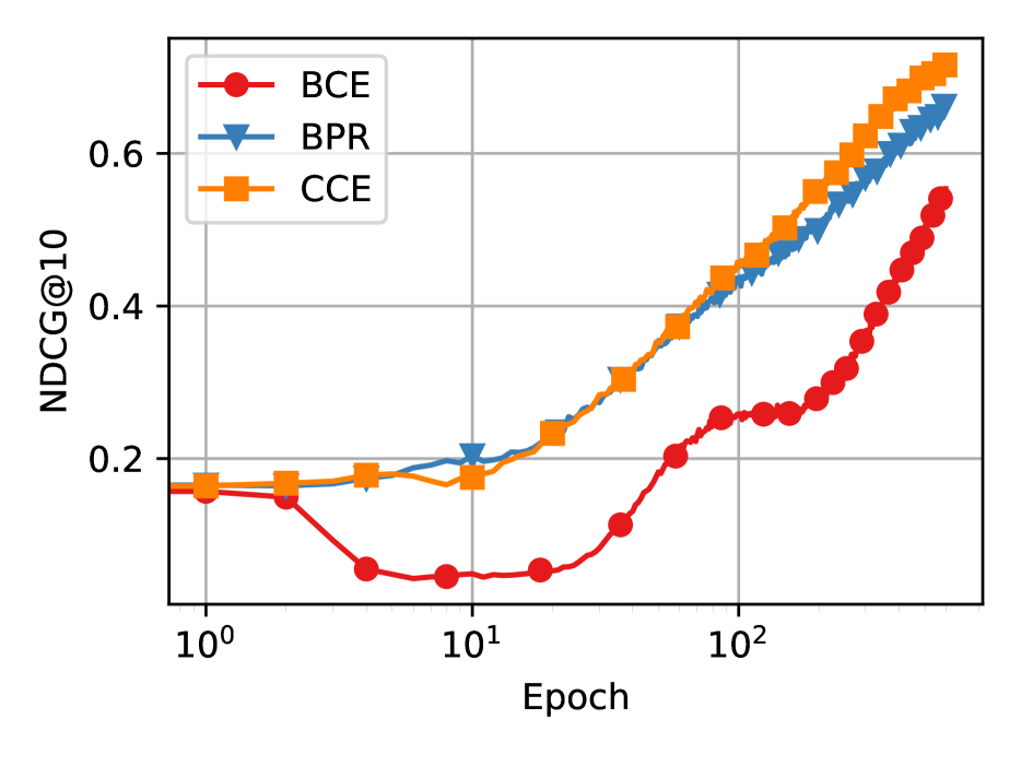
(d) SASRec

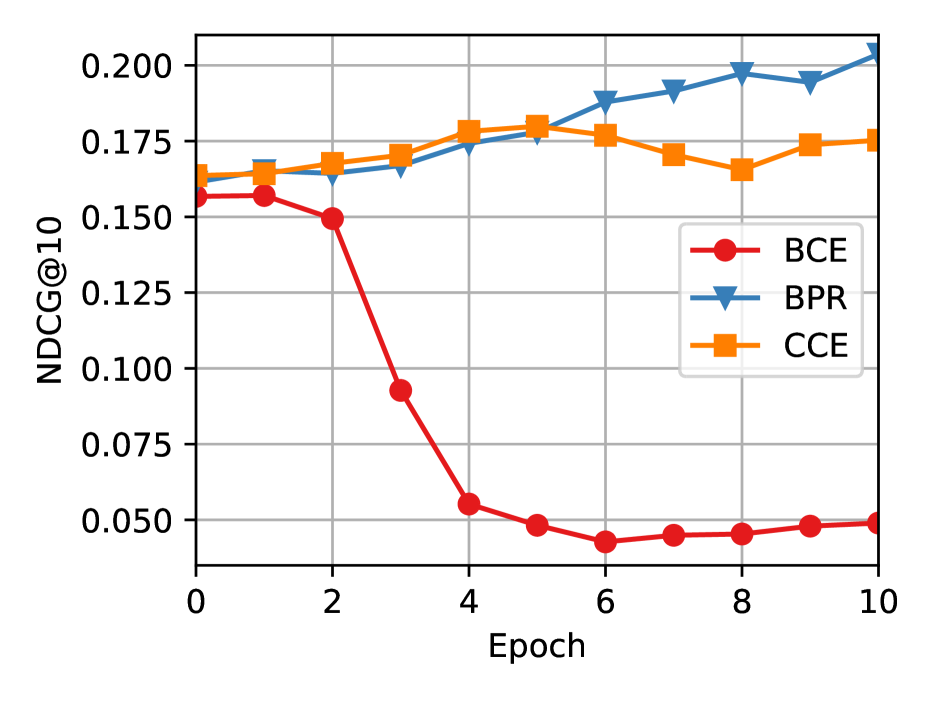
(e) SASRec - Start

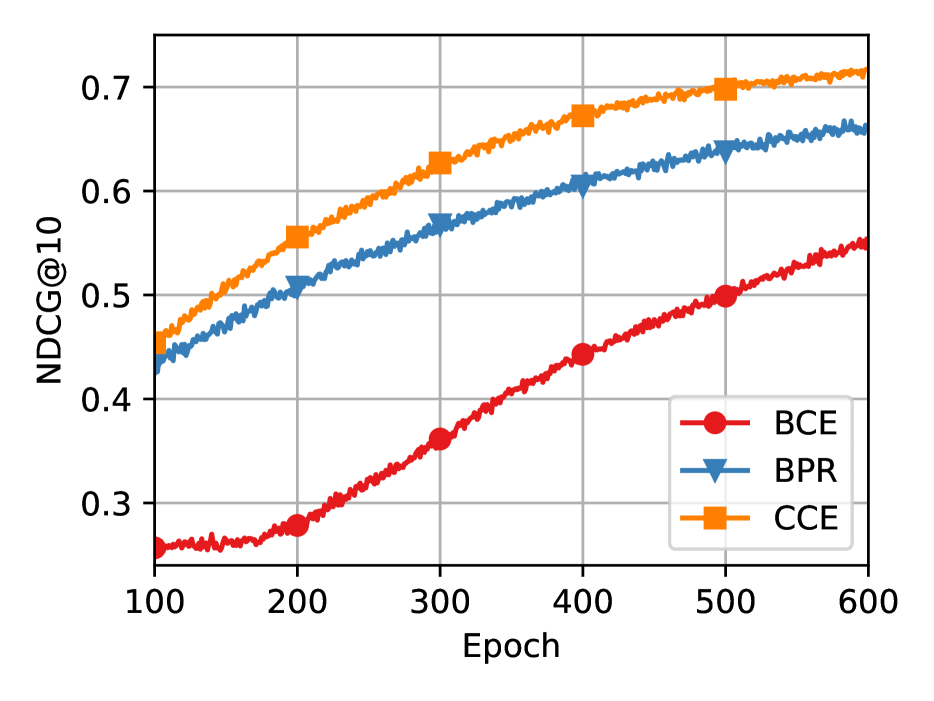
(f) SASRec - End

Figure 20: SASRec and GRU4Rec NDCG@10 during training changing loss, using 100 negative items on Foursquare dataset.

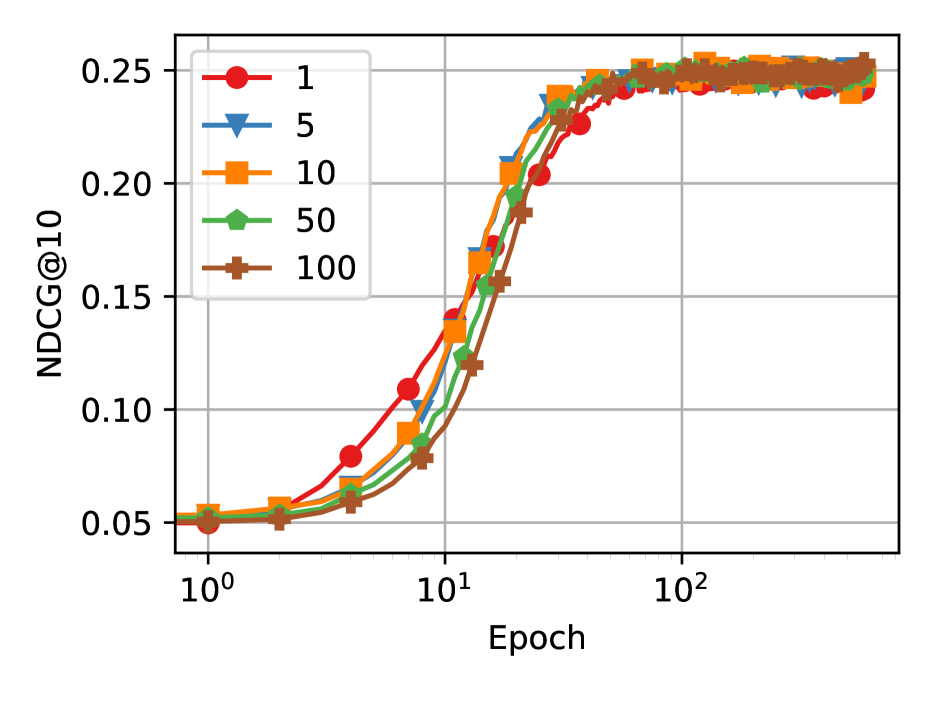
(a) NCF

(b) LightGCN

Figure 21: NCF and LightGCN NDCG@10 during training changing number of negative items, using BCE loss on ML-1M dataset.

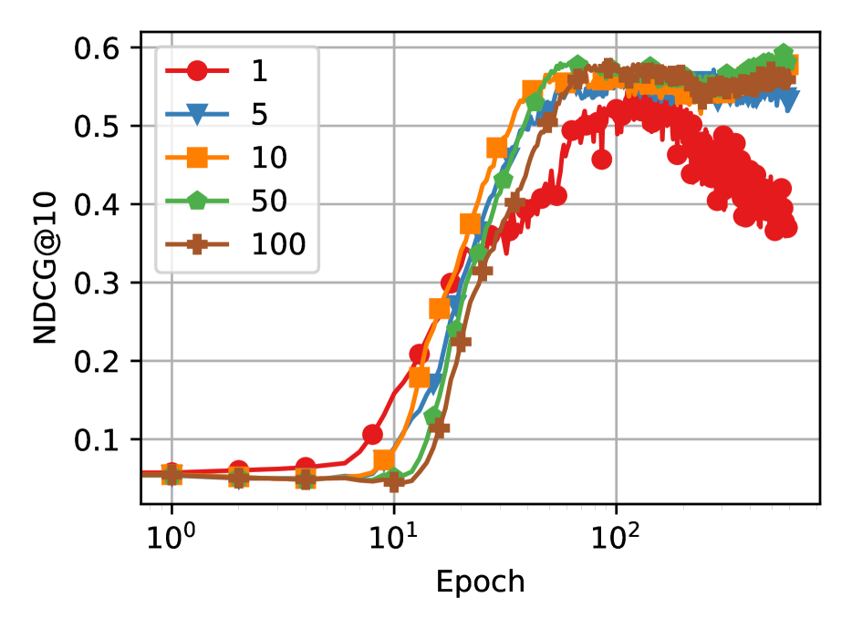
(a) NCF

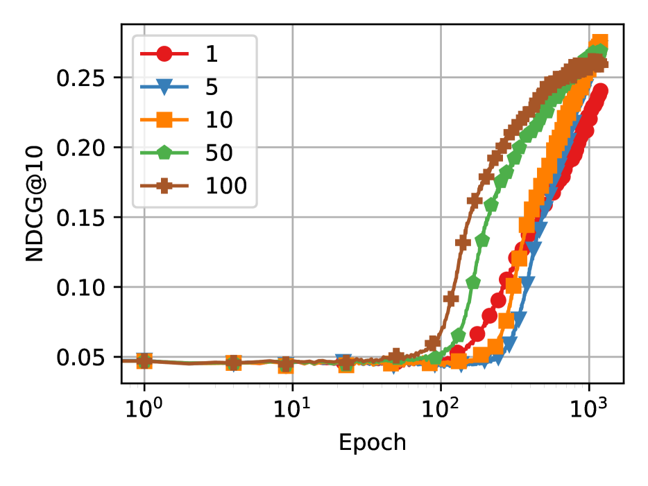
(b) LightGCN

Figure 22: NCF and LightGCN NDCG@10 during training changing number of negative items, using BCE loss on Amazon Beauty dataset.

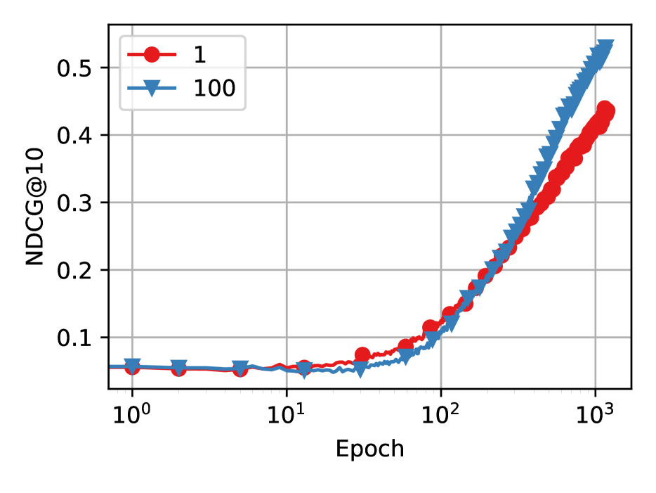
(a) NCF

(b) LightGCN

Figure 23: NCF and LightGCN NDCG@10 during training changing number of negative items, using BCE loss on Foursquare-NYC dataset.

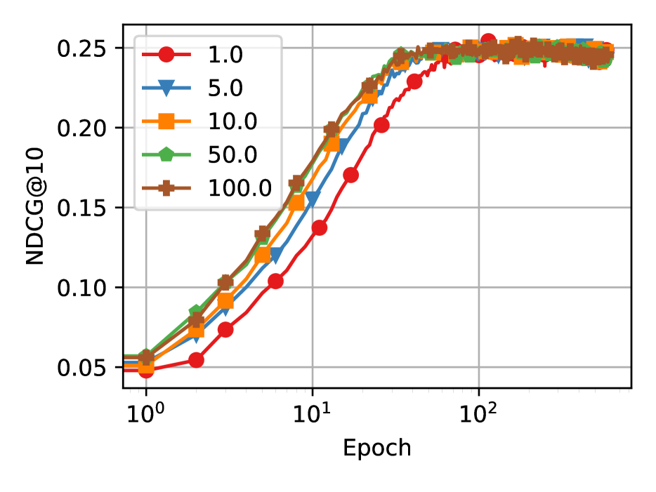
(a) NCF

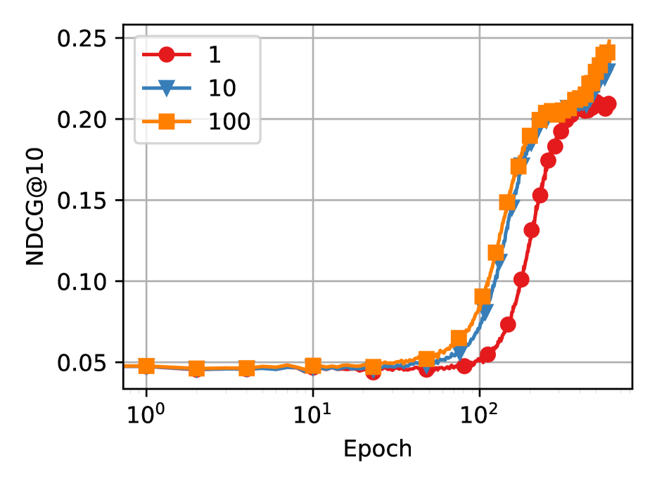
(b) LightGCN

Figure 24: NCF and LightGCN NDCG@10 during training changing number of negative items, using BPR loss on ML-1M dataset.

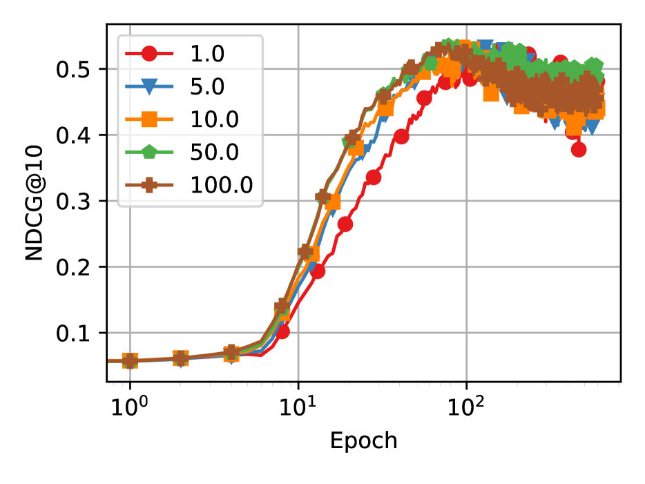
(a) NCF

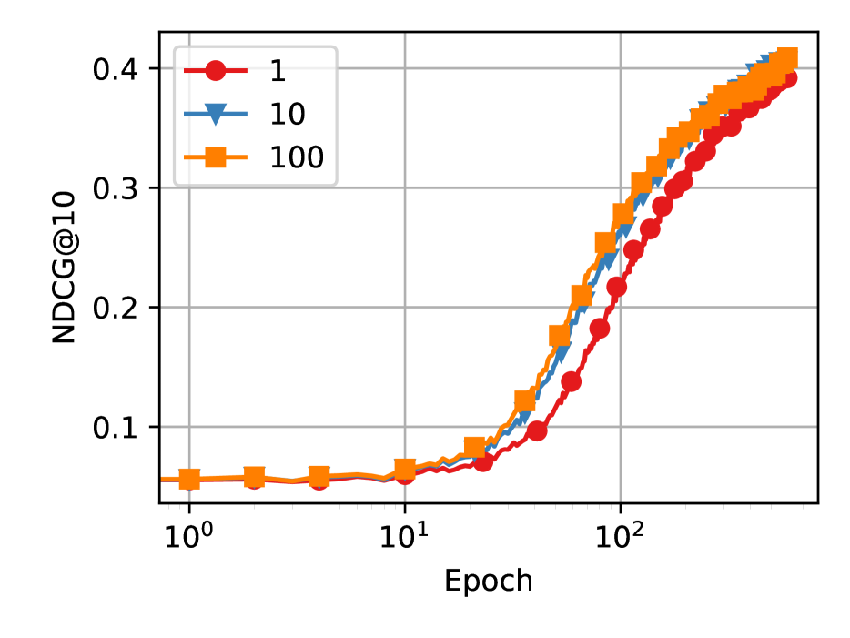
(b) LightGCN

Figure 25: NCF and LightGCN NDCG@10 during training changing number of negative items, using BPR loss on Amazon Beauty dataset.

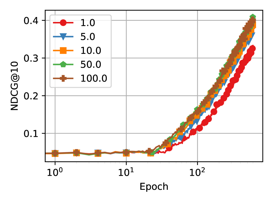
(a) NCF

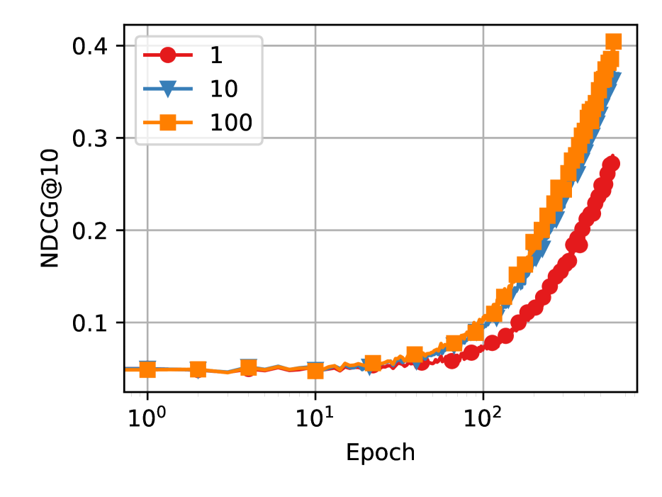
(b) LightGCN

Figure 26: NCF and LightGCN NDCG@10 during training changing number of negative items, using BPR loss on Foursquare-NYC dataset.

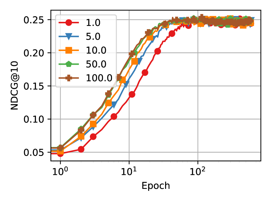
(a) NCF

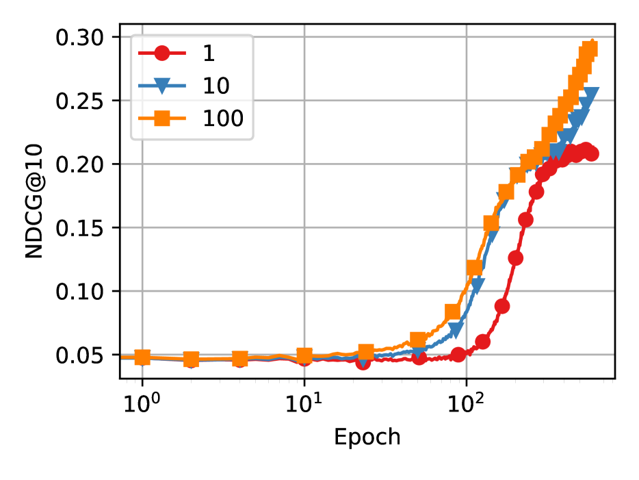
(b) LightGCN

Figure 27: NCF and LightGCN NDCG@10 during training changing number of negative items, using CCE loss on ML-1M dataset.

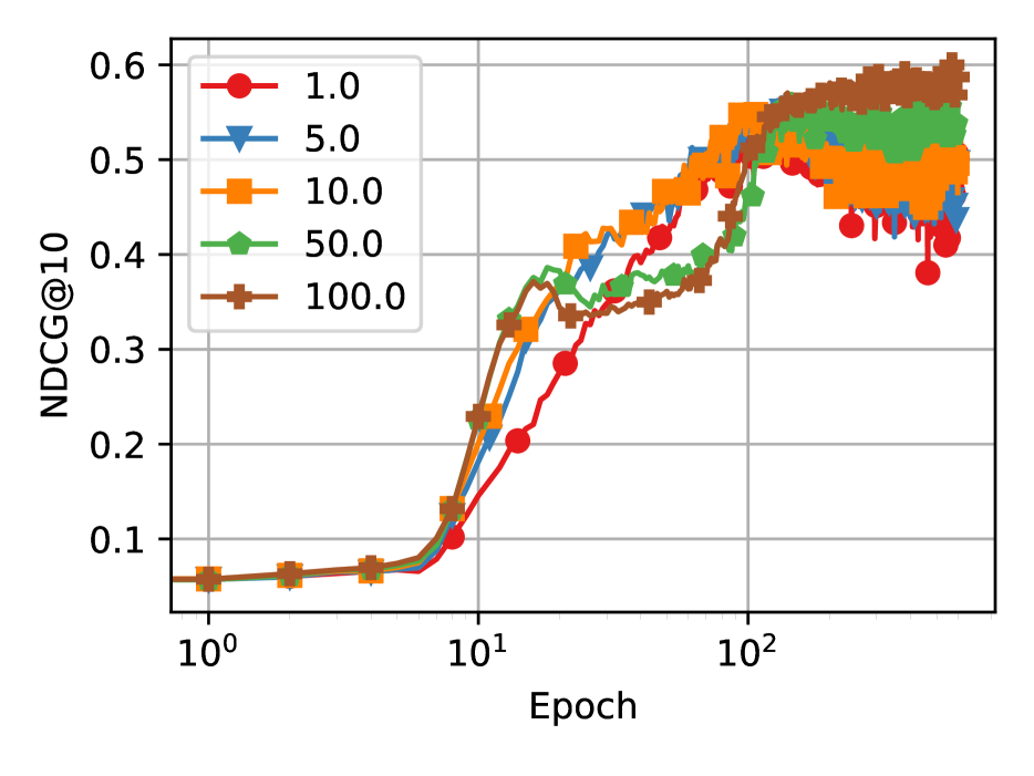
(a) NCF

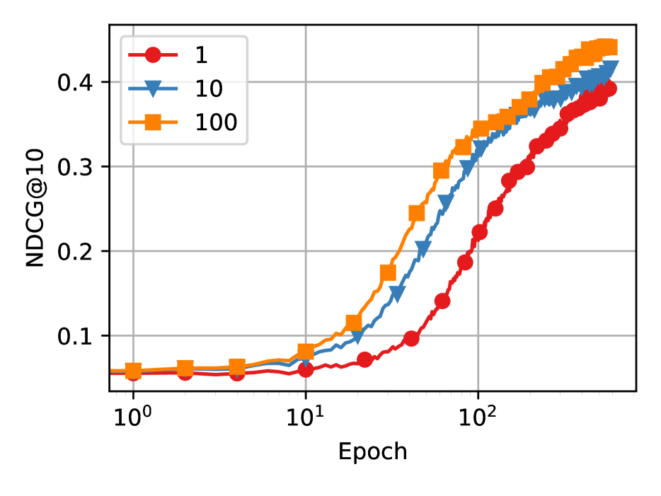
(b) LightGCN

Figure 28: NCF and LightGCN NDCG@10 during training changing number of negative items, using CCE loss on Amazon Beauty dataset.

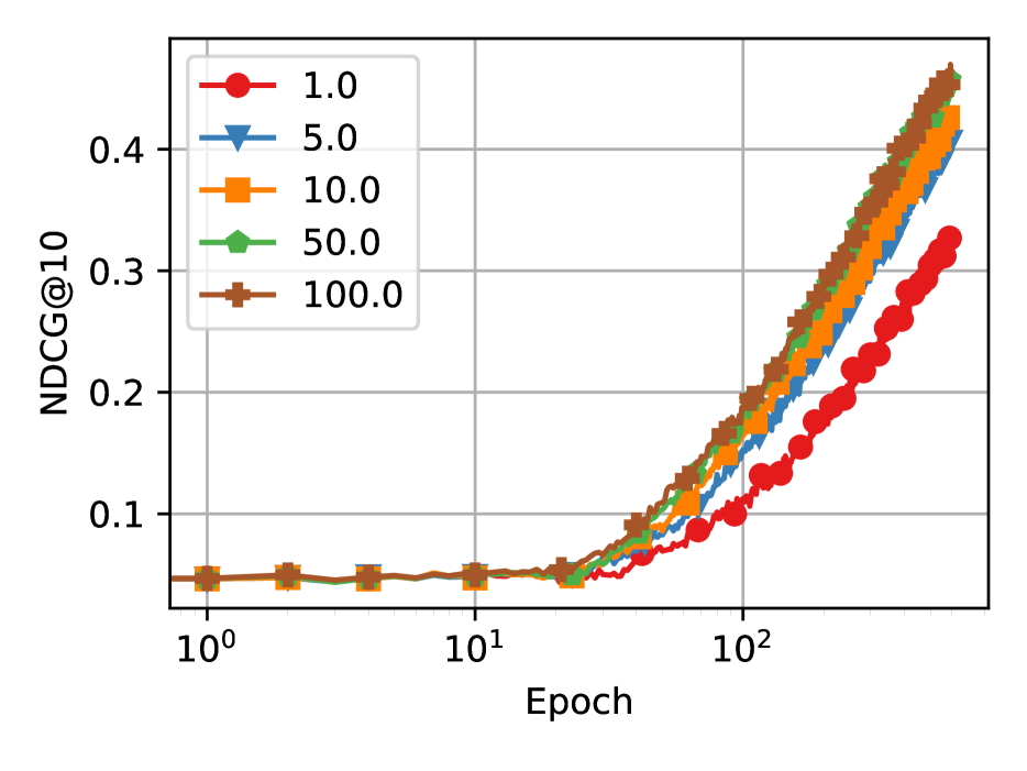
(a) NCF

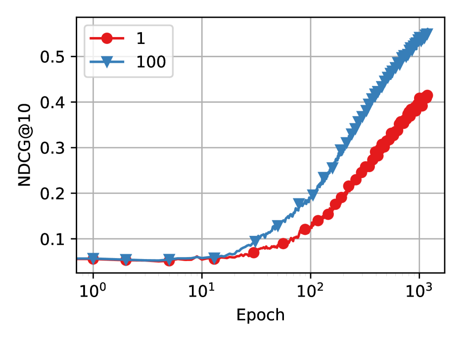
(b) LightGCN

Figure 29: NCF and LightGCN NDCG@10 during training changing number of negative items, using CCE loss on Foursquare-NYC dataset.

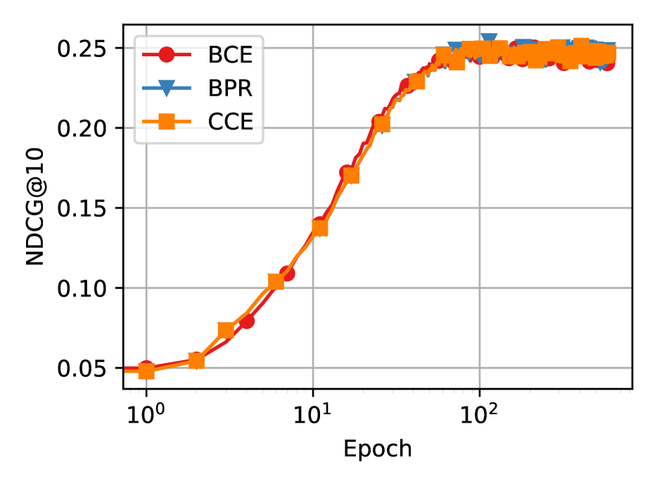
(a) NCF

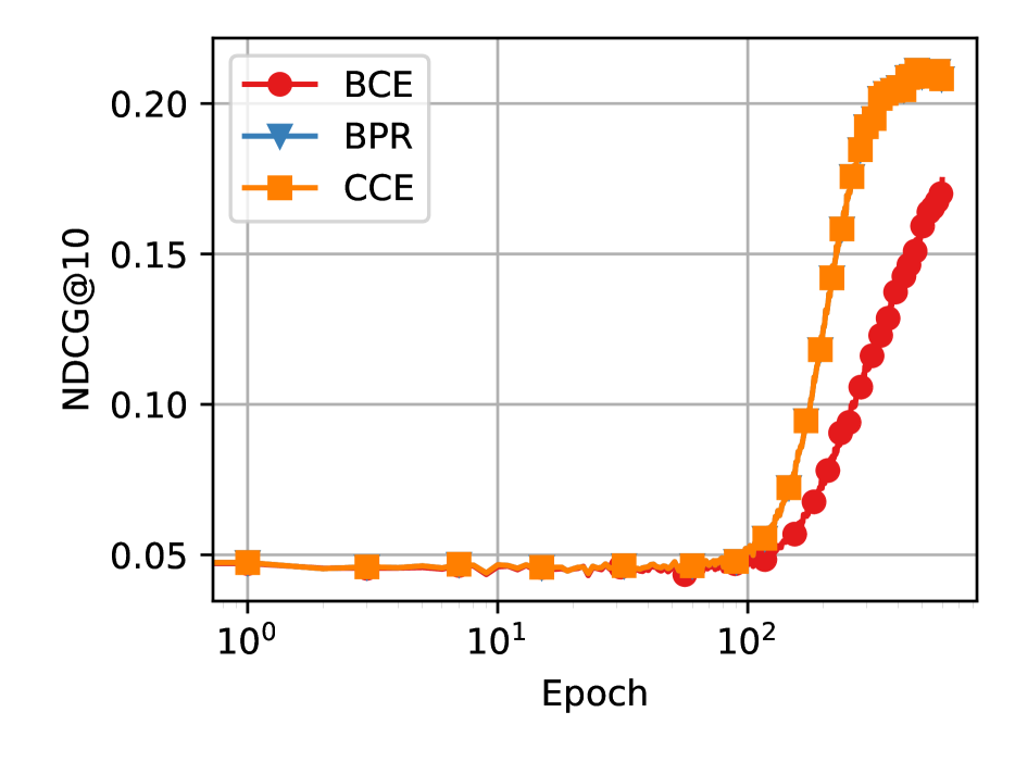
(b) LightGCN

Figure 30: NCF and LightGCN NDCG@10 during training changing loss, using 1 negative item on ML-1M dataset.

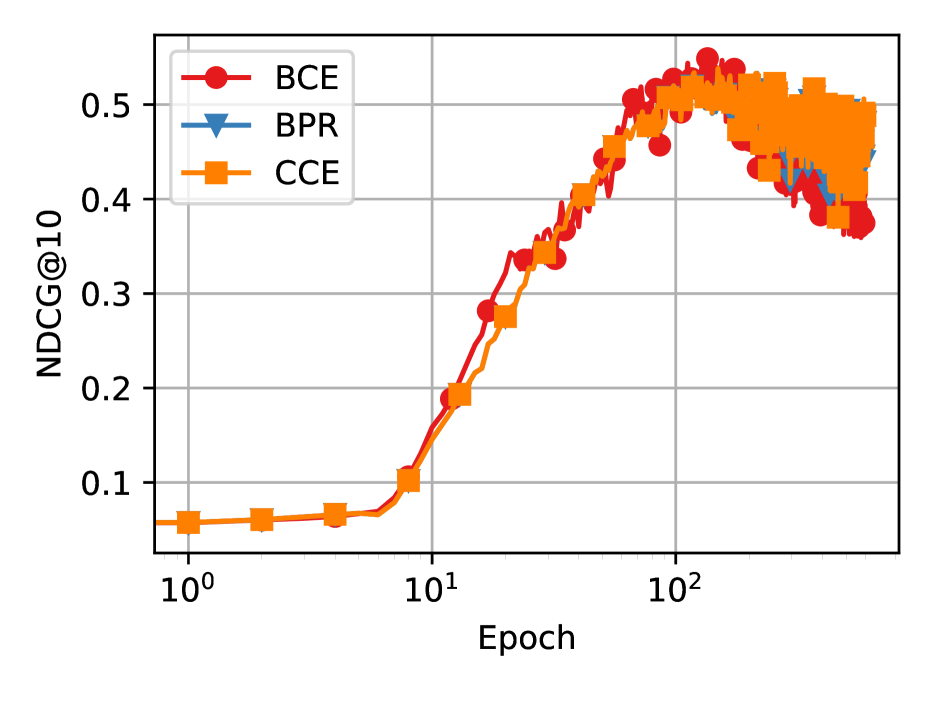
(a) NCF

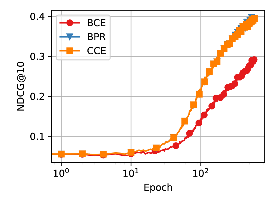
(b) LightGCN

Figure 31: NCF and LightGCN NDCG@10 during training changing loss, using 1 negative item on Amazon Beauty dataset.

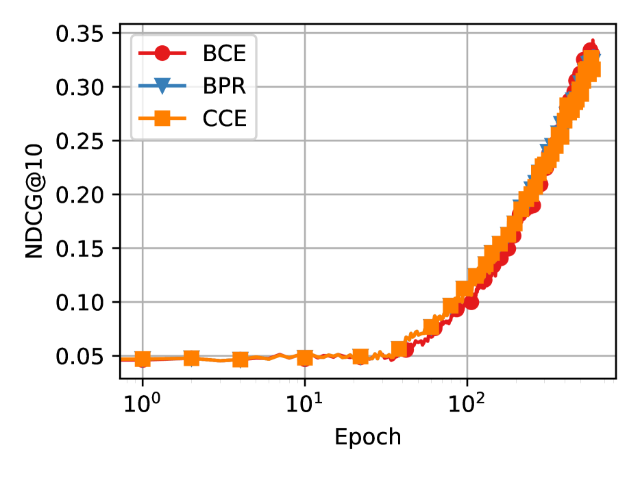
(a) NCF

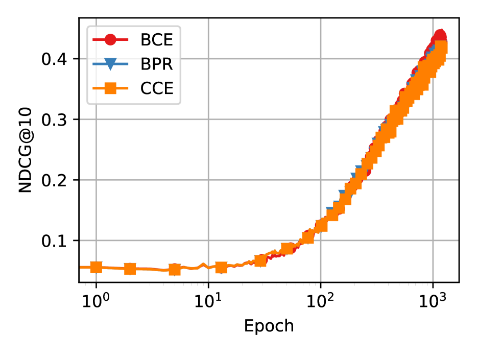
(b) LightGCN

Figure 32: NCF and LightGCN NDCG@10 during training changing loss, using 1 negative item on Foursquare-NYC dataset.

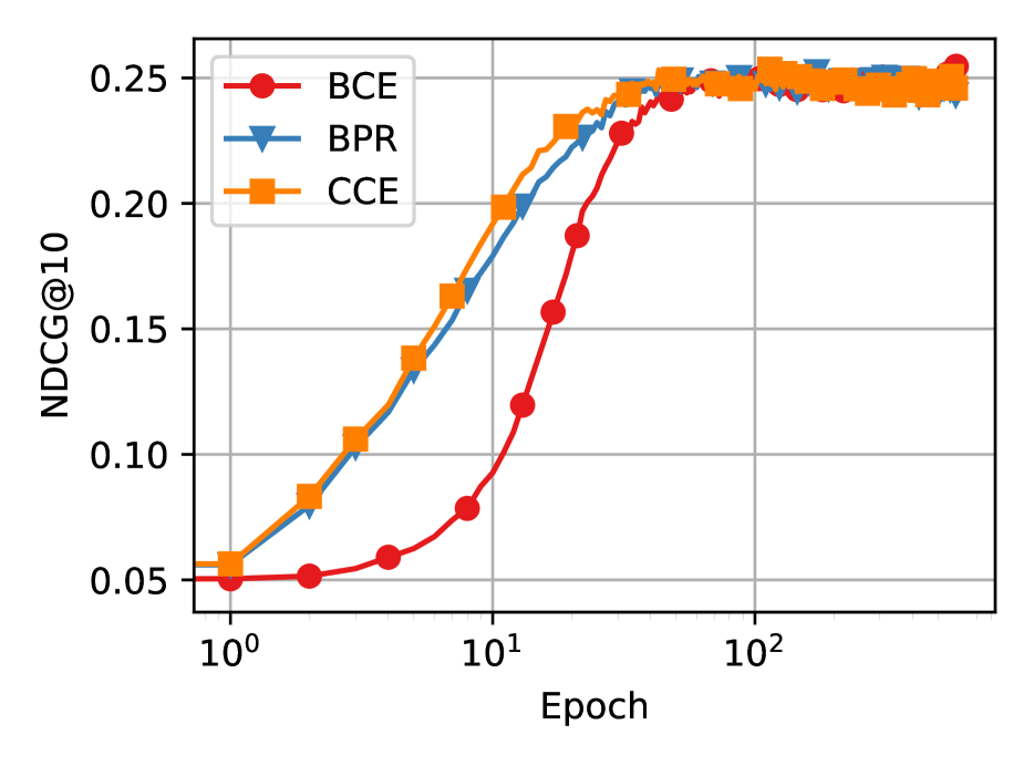
(a) NCF

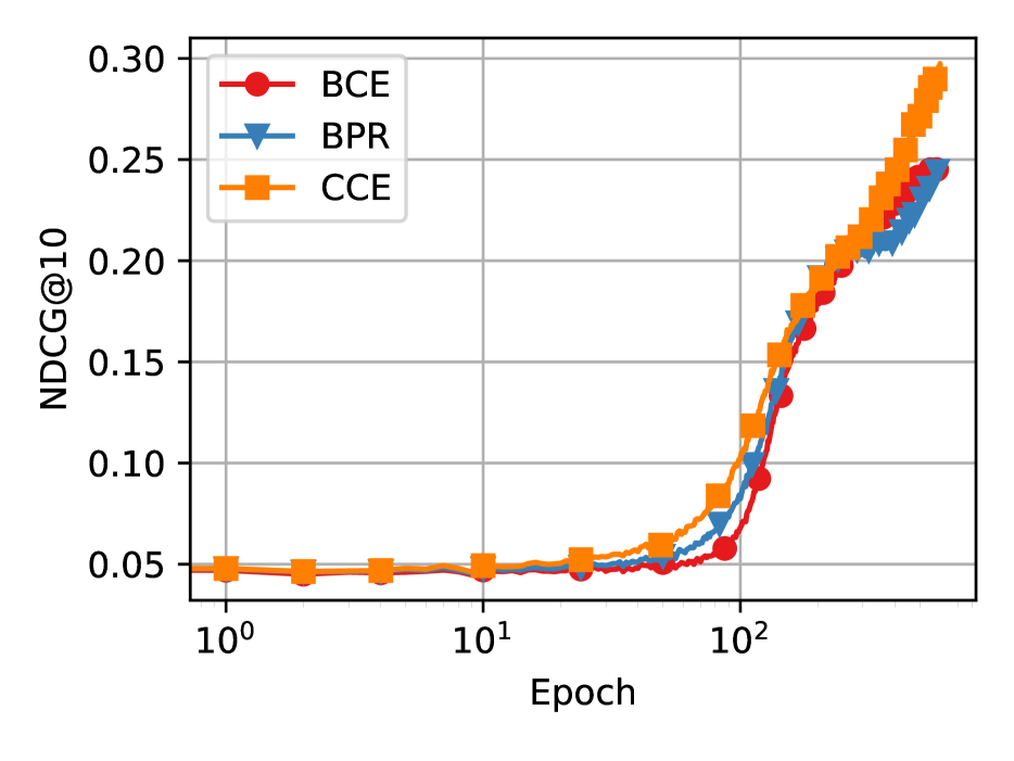
(b) LightGCN

Figure 33: NCF and LightGCN NDCG@10 during training changing loss, using 100 negative items on ML-1M dataset.

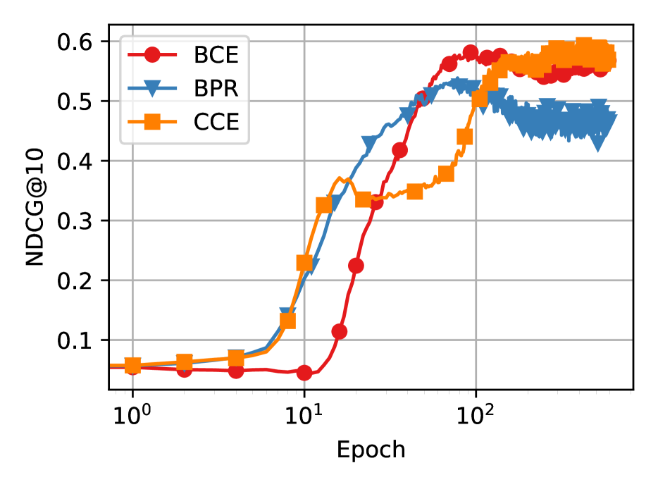
(a) NCF

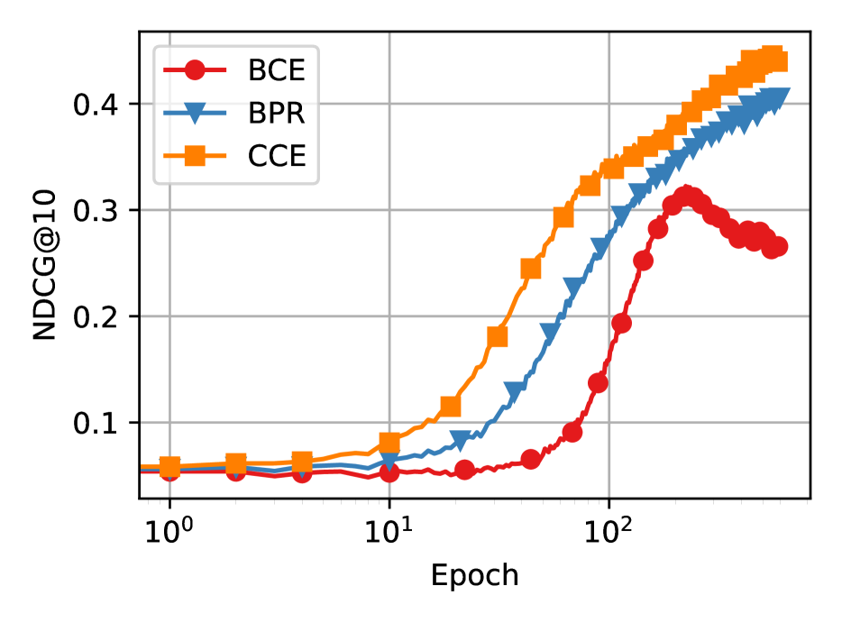
(b) LightGCN

Figure 34: NCF and LightGCN NDCG@10 during training changing loss, using 100 negative items on Amazon Beauty dataset.

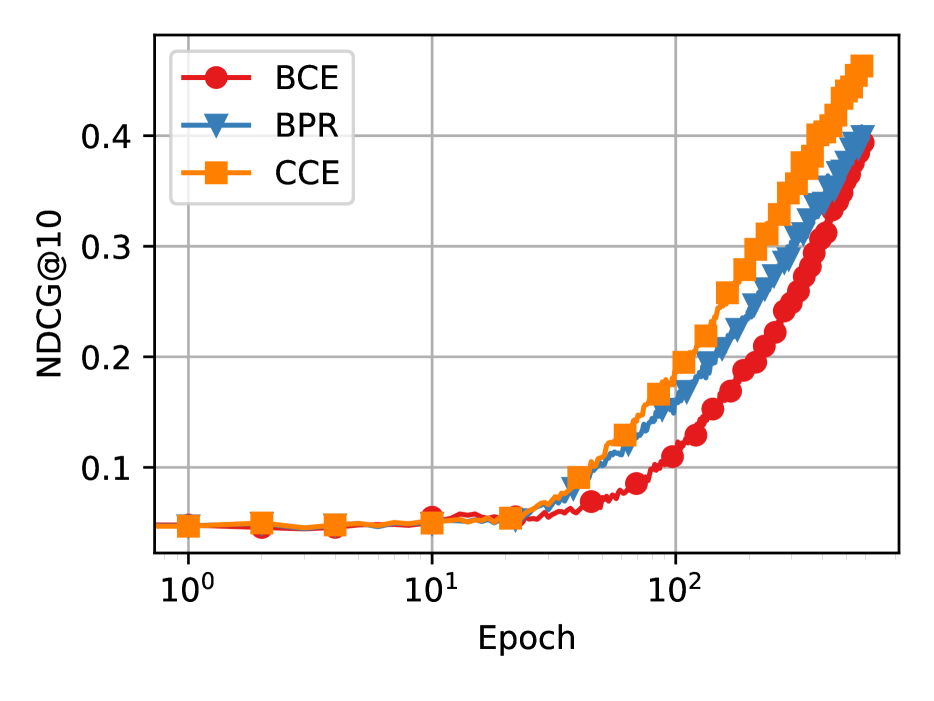
(a) NCF

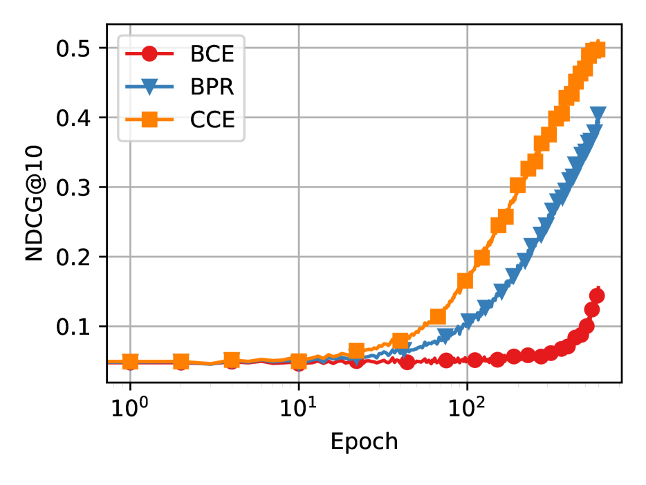
(b) LightGCN

Figure 35: NCF and LightGCN NDCG@10 during training changing loss, using 100 negative items on Foursquare dataset.

References

- Baldi and Lu, (2012) Baldi, P. and Lu, Z. (2012). Complex-valued autoencoders. Neural Networks, 33:136–147.
- Bruch et al., (2019) Bruch, S., Wang, X., Bendersky, M., and Najork, M. (2019). An analysis of the softmax cross entropy loss for learning-to-rank with binary relevance. In Proceedings of the 2019 ACM SIGIR international conference on theory of information retrieval, pages 75–78.
- Burges, (2010) Burges, C. J. C. (2010). From RankNet to LambdaRank to LambdaMART: An overview. Technical report, Microsoft Research.
- Chen et al., (2022) Chen, J., Lian, D., Jin, B., Zheng, K., and Chen, E. (2022). Learning recommenders for implicit feedback with importance resampling. In Proceedings of the ACM Web Conference 2022, WWW ’22, page 1997–2005, New York, NY, USA. Association for Computing Machinery.
- Dallmann et al., (2021) Dallmann, A., Zoller, D., and Hotho, A. (2021). A case study on sampling strategies for evaluating neural sequential item recommendation models. In Proceedings of the 15th ACM Conference on Recommender Systems, RecSys ’21, page 505–514, New York, NY, USA. Association for Computing Machinery.
- de Souza Pereira Moreira et al., (2021) de Souza Pereira Moreira, G., Rabhi, S., Lee, J. M., Ak, R., and Oldridge, E. (2021). Transformers4rec: Bridging the gap between nlp and sequential / session-based recommendation. In Proceedings of the 15th ACM Conference on Recommender Systems, RecSys ’21, page 143–153, New York, NY, USA. Association for Computing Machinery.
- Ding et al., (2020) Ding, J., Quan, Y., Yao, Q., Li, Y., and Jin, D. (2020). Simplify and robustify negative sampling for implicit collaborative filtering. In Proceedings of the 34th International Conference on Neural Information Processing Systems, NIPS ’20, Red Hook, NY, USA. Curran Associates Inc.
- Harper and Konstan, (2015) Harper, F. M. and Konstan, J. A. (2015). The movielens datasets: History and context. ACM Trans. Interact. Intell. Syst., 5(4).
- He et al., (2020) He, X., Deng, K., Wang, X., Li, Y., Zhang, Y., and Wang, M. (2020). Lightgcn: Simplifying and powering graph convolution network for recommendation. In Proceedings of the 43rd International ACM SIGIR Conference on Research and Development in Information Retrieval, SIGIR ’20, page 639–648, New York, NY, USA. Association for Computing Machinery.
- He et al., (2017) He, X., Liao, L., Zhang, H., Nie, L., Hu, X., and Chua, T.-S. (2017). Neural collaborative filtering. In Proceedings of the 26th international conference on world wide web, pages 173–182.
- Hidasi et al., (2016) Hidasi, B., Karatzoglou, A., Baltrunas, L., and Tikk, D. (2016). Session-based recommendations with recurrent neural networks. In International Conference on Learning Representations (ICLR).
- Hu et al., (2008) Hu, Y., Koren, Y., and Volinsky, C. (2008). Collaborative filtering for implicit feedback datasets. In 2008 Eighth IEEE international conference on data mining, pages 263–272. Ieee.
- Järvelin and Kekäläinen, (2002) Järvelin, K. and Kekäläinen, J. (2002). Cumulated gain-based evaluation of ir techniques. ACM Trans. Inf. Syst., 20(4):422–446.
- Kang and McAuley, (2018) Kang, W. and McAuley, J. (2018). Self-attentive sequential recommendation. In 2018 IEEE International Conference on Data Mining (ICDM), pages 197–206, Los Alamitos, CA, USA. IEEE Computer Society.
- Koren et al., (2009) Koren, Y., Bell, R., and Volinsky, C. (2009). Matrix factorization techniques for recommender systems. Computer, 42(8):30–37.
- Krichene and Rendle, (2022) Krichene, W. and Rendle, S. (2022). On sampled metrics for item recommendation. Commun. ACM, 65(7):75–83.
- Lee and Seung, (1999) Lee, D. D. and Seung, H. S. (1999). Learning the parts of objects by non-negative matrix factorization. nature, 401(6755):788–791.
- Li et al., (2017) Li, J., Ren, P., Chen, Z., Ren, Z., Lian, T., and Ma, J. (2017). Neural attentive session-based recommendation. In Proceedings of the 2017 ACM on Conference on Information and Knowledge Management, CIKM ’17, page 1419–1428, New York, NY, USA. Association for Computing Machinery.
- Lian et al., (2020) Lian, D., Liu, Q., and Chen, E. (2020). Personalized ranking with importance sampling. In Proceedings of The Web Conference 2020, pages 1093–1103.
- Liu and Wang, (2023) Liu, B. and Wang, B. (2023). Bayesian negative sampling for recommendation. In 2023 IEEE 39th International Conference on Data Engineering (ICDE), pages 749–761. IEEE.
- McAuley et al., (2015) McAuley, J., Targett, C., Shi, Q., and van den Hengel, A. (2015). Image-based recommendations on styles and substitutes. In Proceedings of the 38th International ACM SIGIR Conference on Research and Development in Information Retrieval, SIGIR ’15, page 43–52, New York, NY, USA. Association for Computing Machinery.
- Palagi, (2019) Palagi, L. (2019). Global optimization issues in deep network regression: an overview. J. Glob. Optim., 73(2):239–277.
- Pellegrini et al., (2022) Pellegrini, R., Zhao, W., and Murray, I. (2022). Don’t recommend the obvious: estimate probability ratios. In Proceedings of the 16th ACM Conference on Recommender Systems, RecSys ’22, page 188–197, New York, NY, USA. Association for Computing Machinery.
- (24) Petrov, A. and Macdonald, C. (2023a). Rss: Effective and efficient training for sequential recommendation using recency sampling. ACM Trans. Recomm. Syst. Just Accepted.
- (25) Petrov, A. V. and Macdonald, C. (2023b). gsasrec: Reducing overconfidence in sequential recommendation trained with negative sampling. In Proceedings of the 17th ACM Conference on Recommender Systems, RecSys ’23, page 116–128, New York, NY, USA. Association for Computing Machinery.
- Pu et al., (2024) Pu, Y., Chen, X., Huang, X., Chen, J., Lian, D., and Chen, E. (2024). Learning-efficient yet generalizable collaborative filtering for item recommendation. In Forty-first International Conference on Machine Learning (ICML).
- Rajput et al., (2023) Rajput, S., Mehta, N., Singh, A., Hulikal Keshavan, R., Vu, T., Heldt, L., Hong, L., Tay, Y., Tran, V., Samost, J., Kula, M., Chi, E., and Sathiamoorthy, M. (2023). Recommender systems with generative retrieval. In Oh, A., Naumann, T., Globerson, A., Saenko, K., Hardt, M., and Levine, S., editors, Advances in Neural Information Processing Systems, volume 36, pages 10299–10315. Curran Associates, Inc.
- Rendle, (2022) Rendle, S. (2022). Item Recommendation from Implicit Feedback, pages 143–171. Springer US, New York, NY.
- Rendle and Freudenthaler, (2014) Rendle, S. and Freudenthaler, C. (2014). Improving pairwise learning for item recommendation from implicit feedback. In Proceedings of the 7th ACM International Conference on Web Search and Data Mining, WSDM ’14, page 273–282, New York, NY, USA. Association for Computing Machinery.
- Rendle et al., (2009) Rendle, S., Freudenthaler, C., Gantner, Z., and Schmidt-Thieme, L. (2009). Bpr: Bayesian personalized ranking from implicit feedback. In Proceedings of the Twenty-Fifth Conference on Uncertainty in Artificial Intelligence, UAI ’09, page 452–461, Arlington, Virginia, USA. AUAI Press.
- Shi et al., (2023) Shi, W., Chen, J., Feng, F., Zhang, J., Wu, J., Gao, C., and He, X. (2023). On the theories behind hard negative sampling for recommendation. In Proceedings of the ACM Web Conference 2023, pages 812–822.
- Sun et al., (2019) Sun, F., Liu, J., Wu, J., Pei, C., Lin, X., Ou, W., and Jiang, P. (2019). Bert4rec: Sequential recommendation with bidirectional encoder representations from transformer. In Proceedings of the 28th ACM International Conference on Information and Knowledge Management, CIKM ’19, page 1441–1450, New York, NY, USA. Association for Computing Machinery.
- Tang and Wang, (2018) Tang, J. and Wang, K. (2018). Personalized top-n sequential recommendation via convolutional sequence embedding. In Proceedings of the Eleventh ACM International Conference on Web Search and Data Mining, WSDM ’18, page 565–573, New York, NY, USA. Association for Computing Machinery.
- Vaswani et al., (2017) Vaswani, A., Shazeer, N., Parmar, N., Uszkoreit, J., Jones, L., Gomez, A. N., Kaiser, L. u., and Polosukhin, I. (2017). Attention is all you need. In Guyon, I., Luxburg, U. V., Bengio, S., Wallach, H., Fergus, R., Vishwanathan, S., and Garnett, R., editors, Advances in Neural Information Processing Systems, volume 30. Curran Associates, Inc.
- Wei et al., (2022) Wei, H., Xie, R., Cheng, H., Feng, L., An, B., and Li, Y. (2022). Mitigating neural network overconfidence with logit normalization. In International conference on machine learning, pages 23631–23644. PMLR.
- Weston et al., (2011) Weston, J., Bengio, S., and Usunier, N. (2011). Wsabie: scaling up to large vocabulary image annotation. In Proceedings of the Twenty-Second International Joint Conference on Artificial Intelligence - Volume Volume Three, IJCAI’11, page 2764–2770. AAAI Press.
- Wu et al., (2024) Wu, J., Wang, X., Gao, X., Chen, J., Fu, H., and Qiu, T. (2024). On the effectiveness of sampled softmax loss for item recommendation. ACM Trans. Inf. Syst., 42(4).
- Xia et al., (2008) Xia, F., Liu, T.-Y., Wang, J., Zhang, W., and Li, H. (2008). Listwise approach to learning to rank: theory and algorithm. In Proceedings of the 25th international conference on Machine learning, pages 1192–1199.
- Xu et al., (2024) Xu, C., Zhu, Z., Wang, J., Wang, J., and Zhang, W. (2024). Understanding the role of cross-entropy loss in fairly evaluating large language model-based recommendation.
- Yang et al., (2015) Yang, D., Zhang, D., Zheng, V. W., and Yu, Z. (2015). Modeling user activity preference by leveraging user spatial temporal characteristics in lbsns. IEEE Transactions on Systems, Man, and Cybernetics: Systems, 45(1):129–142.
- Yang and Koyejo, (2020) Yang, F. and Koyejo, S. (2020). On the consistency of top-k surrogate losses. In International Conference on Machine Learning, pages 10727–10735. PMLR.
- Yuan et al., (2016) Yuan, F., Guo, G., Jose, J. M., Chen, L., Yu, H., and Zhang, W. (2016). Lambdafm: Learning optimal ranking with factorization machines using lambda surrogates. In Proceedings of the 25th ACM International on Conference on Information and Knowledge Management, CIKM ’16, page 227–236, New York, NY, USA. Association for Computing Machinery.
- Zhang et al., (2013) Zhang, W., Chen, T., Wang, J., and Yu, Y. (2013). Optimizing top-n collaborative filtering via dynamic negative item sampling. In Proceedings of the 36th International ACM SIGIR Conference on Research and Development in Information Retrieval, SIGIR ’13, page 785–788, New York, NY, USA. Association for Computing Machinery.
- Zhao et al., (2023) Zhao, Y., Chen, R., Lai, R., Han, Q., Song, H., and Chen, L. (2023). Augmented negative sampling for collaborative filtering. In Proceedings of the 17th ACM Conference on Recommender Systems, RecSys ’23, page 256–266, New York, NY, USA. Association for Computing Machinery.
- Zhou et al., (2020) Zhou, K., Wang, H., Zhao, W. X., Zhu, Y., Wang, S., Zhang, F., Wang, Z., and Wen, J.-R. (2020). S3-rec: Self-supervised learning for sequential recommendation with mutual information maximization. In Proceedings of the 29th ACM International Conference on Information & Knowledge Management, CIKM ’20, page 1893–1902, New York, NY, USA. Association for Computing Machinery.
- Zhu et al., (2022) Zhu, Q., Zhang, H., He, Q., and Dou, Z. (2022). A gain-tuning dynamic negative sampler for recommendation. In Proceedings of the ACM Web Conference 2022, WWW ’22, page 277–285, New York, NY, USA. Association for Computing Machinery.
- Zhuo et al., (2022) Zhuo, J., Zhu, Q., Yue, Y., and Zhao, Y. (2022). Learning explicit user interest boundary for recommendation. In Proceedings of the ACM Web Conference 2022, WWW ’22, page 193–202, New York, NY, USA. Association for Computing Machinery.