Gravitational reheating formulas and bounds in oscillating backgrounds II: Constraints on the spectral index and gravitational dark matter production

Abstract

The reheating temperature plays a crucial role in the early universe’s evolution, marking the transition from inflation to the radiation-dominated era. It directly impacts the number of $e$-folds and, consequently, the observable parameters of inflation, such as the spectral index of scalar perturbations. By establishing a relationship between the gravitational reheating temperature and the spectral index, we can derive constraints on inflationary models. Specifically, the range of viable reheating temperatures imposes bounds on the spectral index, which can then be compared with observational data, such as those from the Planck satellite, to test the consistency of various models with cosmological observations. Additionally, in the context of dark matter production, we demonstrate that gravitational reheating provides a viable mechanism when there is a relationship between the mass of the dark matter particles and the mass of the particles responsible for reheating. This connection offers a pathway to link dark matter genesis with inflationary and reheating parameters, allowing for a unified perspective on early universe dynamics.

I Introduction

The relation between the reheating temperature and the spectral index of scalar perturbations plays a crucial role in understanding the dynamics of the early universe, particularly in the context of inflationary cosmology Guth (1981); Linde (1982). Inflation, a rapid expansion of the universe in its earliest moments, produces scalar perturbations, which later evolve into the large-scale structures we observe today, see for instance Refs. Barrow and Turner (1981); Spokoiny (1984); Steinhardt and Turner (1984); Lucchin and Matarrese (1985); Hawking (1985); Lyth (1985); Belinsky et al. (1985); Mijic et al. (1986); Khalfin (1986); Silk and Turner (1987); Mijic et al. (1986); Burd and Barrow (1988); Olive (1990); Ford (1989); Adams et al. (1991); Freese et al. (1990); Wang (1991); Polarski and Starobinsky (1992); Liddle and Lyth (1992); Linde (1994); Barrow (1993, 1994); Vilenkin (1994); Peter et al. (1994); Sasaki and Stewart (1996); Barrow and Parsons (1995); Lidsey et al. (1997); Parsons and Barrow (1995); Liddle (1998); Guth (2000); Riotto (2003); Feinstein (2002); Ashcroft et al. (2004); Boubekeur and Lyth (2005); Conlon and Quevedo (2006); Ferraro and Fiorini (2007); Cheung et al. (2008); Chen et al. (2008); Baumann and Peiris (2009); Koivisto and Mota (2008); Pal et al. (2010); Martin et al. (2014a, b); Sebastiani et al. (2014); Hamada et al. (2014); Freese and Kinney (2015); van de Bruck and Paduraru (2015); van de Bruck and Longden (2016a, b); Ratra (2017); Rubio (2019); Giarè et al. (2019); van de Bruck and Daniel (2021); Forconi et al. (2021); Odintsov et al. (2023); Giarè et al. (2023); Jinno et al. (2024); Garfinkle et al. (2023). The spectral index, $n_{s}$, characterizes the distribution of these perturbations and offers insights into the physics of the inflationary period.

In addition, the number of $e$-folds between the horizon crossing and the end of inflation is influenced by the reheating temperature, $T_{\rm reh}$. Since the spectral index $n_{s}$ depends on this last number of $e$-folds, the reheating temperature impacts the predicted value of $n_{s}$. Higher reheating temperatures generally reduce the duration of the reheating phase, leading to fewer $e$-folds and a lower predicted value of the spectral index, while lower reheating temperatures result in more $e$-folds and a higher spectral index. As a consequence, by studying the connection between $T_{\rm reh}$ and $n_{s}$, different inflationary models can be tested and compared with the observational data, such as the measurements from the Planck satellite Akrami et al. (2020). This relationship serves as a valuable tool for constraining models of inflation, and only those predicting a viable range of $n_{s}$ consistent with observations, are considered plausible.

In the context of gravitational reheating and considering a heavy scalar quantum field conformally coupled to gravity, the created particles must decay into lighter ones to reheat the universe. First, continuing with our previous work de Haro et al. (2024), we derive the formula for the reheating temperature as a function of the decay rate and the mass $m_{\chi}$ of the produced particles, identifying viable values of $m_{\chi}$ and the range of possible reheating temperatures. Using this range and considering the relationship between the reheating temperature and the spectral index, we are able to constrain the latter. Indeed, these spectral index values are more tightly constrained than those obtained experimentally by Planck’s data Akrami et al. (2020).

On the other hand, in the absence of strong couplings between the inflaton and standard particles, gravitational reheating can produce a non-thermal spectrum of particles, including potential dark matter candidates. This mechanism is especially intriguing in models where dark matter particles have minimal interactions with ordinary matter. During gravitational reheating, dark matter production can occur efficiently through gravitational interactions alone, providing a natural and model-independent production pathway. This scenario could help explain the relic density of dark matter observed today without requiring direct couplings to the inflaton field. Having in mind this fact, we investigate the gravitational production of dark matter within the framework of gravitational reheating. Specifically, we consider two distinct scalar fields conformally coupled to gravity, which generate two types of particles with different masses. One type decays into lighter particles, facilitating the reheating of the universe, while the other, a candidate for explaining the dark matter content, does not decay. In this work, we determine the range of particle masses that yield both a viable reheating temperature and a present-day value for the cold dark matter energy density, thereby contributing to a more complete understanding of the dark matter and energy composition of the universe.

The paper is structured as follows: In Section II, we use the Wentzel-Kramers-Brillouin (WKB) method in the complex plane to analytically calculate the $\beta$-Bogoliubov coefficient, the key component for determining particle production. In Section III, we constrain the viable values of the spectral index by relating it to the reheating temperature through the last few $e$-folds. In Section IV, we derive an analytical formula for the reheating temperature when reheating occurs via gravitational particle production. This formula allows us to identify the viable mass range for the produced particles and further constrain the spectral index. Section V addresses the gravitational production of dark matter, where we establish the relationship between the mass of dark matter and that of the scalar field responsible for gravitational reheating. Finally, in Section VI we summarize the present work.

Throughout the manuscript we use natural units, i.e., $\hbar=c=k_{B}=1$, and the reduced Planck’s mass is denoted by $M_{\rm pl}\equiv\frac{1}{\sqrt{8\pi G}}\cong 2.44\times 10^{18}$ GeV.

II Analytic calculation of the energy density of produced particles: The Stokes phenomenon

We consider gravitational reheating through the production of heavy massive particles generated by a spectator scalar field conformally coupled to the Ricci scalar. After their creation, these particles decay into Standard Model particles, which, after thermalization, eventually dominate the inflaton’s energy density, thereby reheating the universe.

The key quantity to calculate is the energy density of the particles produced at the end of inflation Zeldovich and Starobinsky (1971):

$$\langle\rho_{\rm END}\rangle=\frac{m_{\chi}}{2\pi^{2}}\int_{0}^{\infty}k^{2}|\beta_{k}|^{2}dk,$$ (1)

where $\beta_{k}$ is the $\beta$-Bogoliubov coefficient Bogolyubov (1958) and $m_{\chi}$ is the mass of the produced particles, which we will assume to be small compared to the Hubble rate at the end of inflation $H_{\rm END}$.

We focus on the following class of potentials studied in Drewes et al. (2017) (although our analysis can be applied to inflationary models such as Hyperbolic Inflation (HBI), Superconformal $\alpha$-Attractor B Inflation (SABI) or Superconformal $\alpha$-Attractor T Inflation (SATI) Martin et al. (2014b)) which allow for efficient gravitational reheating while maintaining consistency with observational data on the early universe:

$$V_{n}(\varphi)=\lambda M_{\rm pl}^{4}\left(1-e^{-\sqrt{\frac{2}{3}}\frac{\varphi}{M_{\rm pl}}}\right)^{2n}\quad\mbox{with}\qquad n>2,$$ (2)

where $n$ is a natural number and the value of the dimensionless constant $\lambda\sim 3\pi^{2}(1-n_{s})^{2}10^{-9}$ in which $n_{s}\sim 0.96$ is the value of the spectral index of scalar perturbations, is obtained from the power spectrum of scalar perturbations. During oscillations, since close to the minimum, the potential behaves like $\varphi^{2n}$, using the virial theorem we find that the effective Equation of State (EoS) parameter is $w_{\rm eff}(n)=\frac{n-1}{n+1}$ Turner (1983), which is higher than $1/3$ for $n>2$, which ensures that the energy density of the inflation decreases faster than the energy density of the produced particles and their decay products, and thus, this last one eventually will dominate leading to a successful reheating of the universe.

Remark II.1

One can also make viable the cases $n=1$ and $n=2$ assuming that the inflaton decays into relativistic particles of the Standard Model (SM) Garcia et al. (2021); Kaneta et al. (2022). However, this means that the quantum field is coupled to the inflaton field, and thus, this is not exactly what one understand as a ”gravitational particle production” Ford (1987); Chun et al. (2009); Lankinen and Vilja (2017); Haro et al. (2019), where the quantum field is coupled to the Ricci scalar. On the other hand, one can consider that effectively, the reheating occurs due to the coupling with the inflaton field and a quantum field producing the particles of the SM, and also considers another spectator massive quantum field coupled to gravity, which would be a candidate to produce gravitationally dark matter  Jenks et al. (2024); Ema et al. (2018); Chung et al. (2001); Garcia et al. (2020).

Taking into account that when $m_{\chi}\ll H_{\rm END}$, the main contribution of particle production comes from the pure Hubble expansion Hashiba and Yokoyama (2019), we disregard the oscillating effect, and we approximate the scale factor, in the complex plane, by:

$$a(\eta)=\left\{\begin{array}[]{ccc}-\frac{1}{H_{\rm END}\eta}&\mbox{when}&\mathfrak{Re}(\eta)<\eta_{\rm END}\\ &&\\ a_{\rm END}\left[\frac{3n}{n+1}\left(1-\frac{\eta}{\eta_{\rm END}}\right)+\frac{\eta}{\eta_{\rm END}}\right]^{\frac{n+1}{2n-1}}&\mbox{when}&\mathfrak{Re}(\eta)\geq\eta_{\rm END},\end{array}\right.$$ (6)

with $a_{\rm END}=-\frac{1}{H_{\rm END}\eta_{\rm END}}$, being $\eta_{\rm END}<0$. This model depicts a purely de Sitter phase during inflation with a sudden transition to a phase with a constant EoS parameter $w_{\rm eff}(n)=\frac{n-1}{n+1}$. We have to recall that, for a smooth potential as (2), this phase transition is not so abrupt.

On the other hand, the complex WKB approximation tells us that the main contribution of the particle production comes from the turning points (Stokes phenomenon) — in our case points where $\omega_{k}^{2}(\eta)=k^{2}+a^{2}(\eta)m_{\chi}^{2}=0$ — and at the end of inflation Hashiba and Yamada (2021).

II.1 Turning points

The turning points corresponding to the de Sitter phase are $\eta_{c}=\pm i\frac{m_{\chi}}{H_{\rm END}k}$, and since its real part is $0$ they do not belong to the inflationary domain, and thus, they do not contribute to the particle production. The other turning points, corresponding to the other phase, are:

$$\eta_{c}=\frac{3n}{2n-1}\eta_{\rm END}-(-1)^{\frac{2n-1}{2(n+1)}}\left(\frac{n+1}{2n-1}\right)$$

$$\times\eta_{\rm END}\left(\frac{k}{a_{\rm END}m_{\chi}}\right)^{\frac{2n-1}{n+1}}.$$ (7)

Here we can see that for $n=2$, the real part of the turning points is $2\eta_{\rm END}$, which belongs to the inflationary domain, and thus, there is no contribution to the particle production. For the other values of $n$, when $k\gg a_{\rm END}m_{\chi}$, we can see that there are turning points whose real part does not belong to the inflationary domain, and thus, they contribute to the particle production.

Next, we consider only the turning points with positive imaginary part and we take the straight line:

$$\eta=\frac{3n}{2n-1}\eta_{\rm END}-(-1)^{\frac{2n-1}{2(n+1)}}\left(\frac{n+1}{2n-1}\right)$$

$$\times\eta_{\rm END}\left(\frac{k}{a_{\rm END}m_{\chi}}\right)^{\frac{2n-1}{n+1}}\tau,\quad\mbox{with}\quad 0\leq\tau\leq 1.$$ (8)

Over this line $a(\tau)=i\frac{k}{m_{\chi}}\tau^{\frac{n+1}{2n-1}}$, and thus, $\omega_{k}^{2}(\tau)=k^{2}(1-\tau^{\frac{2(n+1)}{2n-1}})$. Therefore, based on the approach described in Landau and Lifshitz (1991), we have:

$$|\beta_{k}|^{2}\cong\exp\left(-4\mathfrak{Im}\int_{\frac{3n}{2n-1}\eta_{\rm END}}^{\eta_{c}}\omega_{k}(z)dz\right),$$ (9)

where $\mathfrak{Im}$ denotes the imaginary part and the integral is performed along the line (II.1). Then, we have:

$$|\beta_{k}|^{2}\cong\exp\left(-c_{n}\left(\frac{k}{H_{\rm END}a_{\rm EDN}}\left(\frac{H_{\rm END}}{m_{\chi}}\right)^{\frac{2n-1}{3n}}\right)^{\frac{3n}{n+1}}\right),$$ (10)

where the value of the dimensionless constant is:

$$c_{n}=4\sin\left(\frac{\pi}{2(n+1)}\right)\frac{n+1}{2n-1}\int_{0}^{1}\sqrt{1-\tau^{\frac{2(n+1)}{2n-1}}}d\tau$$

$$=2\sin\left(\frac{\pi}{2(n+1)}\right)\int_{0}^{1}t^{-\frac{3}{2n+2}}\sqrt{1-t}dt$$

$$=2\sin\left(\frac{\pi}{2(n+1)}\right)B\left(\frac{2n-1}{2n+2},\frac{3}{2}\right),$$ (11)

where $B$ denotes the Euler’s beta function, and from all the turning points with positive imaginary part we have chosen the one which the minimum value of the imaginary part in the exponential of (9) (see for details Section $52$ of Chapter VII of Landau and Lifshitz (1991)).

Finally, its contribution to the energy density is:

$$C_{n}m_{\chi}H_{\rm END}^{3}\left(\frac{m_{\chi}}{H_{\rm END}}\right)^{(2n-1)/n}\left(\frac{a_{\rm END}}{a(t)}\right)^{3},$$ (12)

where

$$C_{n}\cong\frac{1}{2\pi^{2}}\int_{\left(\frac{m_{\chi}}{H_{\rm END}}\right)^{\frac{n+1}{3n}}}^{\infty}x^{2}\exp\left({-c_{n}x^{\frac{3n}{n+1}}}\right)dx$$

$$\cong\frac{1}{2\pi^{2}}\int_{0}^{\infty}x^{2}\exp\left({-c_{n}x^{\frac{3n}{n+1}}}\right)dx.$$ (13)

II.1.1 Case $n=1$

As an example, we calculate:

$$c_{1}=4\sqrt{2}\int_{0}^{1}\sqrt{1-\tau^{4}}d\tau=\sqrt{2}B\left(\frac{1}{4},\frac{3}{2}\right)=\sqrt{2}\frac{\Gamma\left(\frac{1}{4}\right)\Gamma\left(\frac{3}{2}\right)}{\Gamma\left(\frac{7}{4}\right)},$$ (14)

and since $\Gamma\left(\frac{3}{2}\right)=\frac{\sqrt{\pi}}{2}$, and using the duplication formula Abramowitz and Stegun (1965)

$$\Gamma(z)\Gamma\left(z+\frac{1}{2}\right)=2^{1-2z}\sqrt{\pi}\Gamma(2z),$$ (15)

we find $\Gamma\left(\frac{7}{4}\right)=\frac{3\pi}{2\sqrt{2}}\Gamma^{-1}\left(\frac{1}{4}\right)$, and thus, we obtain the same result numerically obtained in Hashiba and Yokoyama (2019) and analytically in the formula (B.4) of Jenks et al. (2024):

$$c_{1}=\frac{2}{3\sqrt{\pi}}\Gamma^{2}\left(\frac{1}{4}\right)\cong 4.9442,$$ (16)

where we have used that $\Gamma\left(\frac{1}{4}\right)\cong 3.6256.$

Once we have calculated $c_{1}$, one has:

$$C_{1}\cong\frac{1}{2\pi^{2}}\int_{0}^{\infty}x^{2}e^{-c_{1}x^{3/2}}dx=\frac{1}{\pi^{2}c_{1}^{2}}\int_{0}^{\infty}y^{5}e^{-y^{2}}dy$$

$$=\frac{1}{\pi^{2}c_{1}^{2}}=\frac{9}{4\pi}\Gamma^{-4}\left(\frac{1}{4}\right)\cong 4\times 10^{-3}.$$ (17)

II.2 End of inflation

Concerning to the end of inflation, $\eta_{\rm END}$, close to this point we make the quadratic approximation:

$$a(\eta)\cong a_{END}+a_{END}^{2}H_{END}(\eta-\eta_{END})$$

$$+\frac{1}{2}a_{END}^{3}H_{END}^{2}(\eta-\eta_{END})^{2},$$ (18)

and up to degree two, we have

$$a^{2}(\eta)\cong a_{END}^{2}+2a_{END}^{3}H_{END}(\eta-\eta_{END})$$

$$+{2}a_{END}^{4}H_{END}^{2}(\eta-\eta_{END})^{2},$$ (19)

and the frequency can be approximated by

$$\omega_{k}^{2}(\eta)\cong k^{2}+\frac{m_{\chi}^{2}a_{END}^{2}}{2}$$

$$+2a_{END}^{4}H_{END}^{2}m_{\chi}^{2}\left(\eta-\frac{3}{2}\eta_{END}\right)^{2},$$ (20)

and defining

$$\tau\equiv\sqrt{\sqrt{2}a^{2}_{\rm END}H_{\rm END}m_{\chi}}\left(\eta-\frac{3}{2}\eta_{\rm END}\right),$$ (21)

the dynamical equation of the $k$-mode is

$$\frac{d^{2}\chi_{k}}{d\tau^{2}}+(\kappa^{2}+\tau^{2})\chi_{k}=0,$$ (22)

where we have introduced the notation $\kappa^{2}=\frac{k^{2}+{a^{2}_{\rm END}m_{\chi}^{2}}/2}{\sqrt{2}a^{2}_{\rm END}H_{\rm END}m_{\chi}}$. Note that for this quadratic frequency the $\beta$-Bogoliubov coefficient is obtained using the well-known formula

$$|\beta_{k}|^{2}=e^{-\pi\kappa^{2}}=\exp\left(-\pi\frac{k^{2}+{a^{2}_{\rm END}m_{\chi}^{2}}/2}{\sqrt{2}a^{2}_{\rm END}H_{\rm END}m_{\chi}}\right)$$

$$\cong\exp\left(-\pi\frac{k^{2}}{\sqrt{2}a^{2}_{\rm END}H_{\rm END}m_{\chi}}\right),$$ (23)

where we have used that $m_{\chi}\ll H_{\rm END}$, and which practically coincides (the difference is the substitution, in the exponential, of $\pi$ by $4$) with the formula (41) obtained in Chung (2003) using the steepest descent method.

This result can be derived as follows. First, recall that the positive frequency modes in the WKB approximation are

$$\phi_{k,+}(\tau)=\frac{1}{(\kappa^{2}+\tau^{2})^{1/4}}e^{-i\int\sqrt{\kappa^{2}+\tau^{2}}d\tau},$$ (24)

and for large values of $|\tau|$ ($|\tau|\gg\kappa$), one can make the approximations $(\kappa^{2}+\tau^{2})^{1/4}\cong|\tau|^{1/2}$ and $\sqrt{\kappa^{2}+\tau^{2}}\cong|\tau|\left(1+\frac{\kappa^{2}}{2\tau^{2}}\right)$, obtaining

$$\left\{\begin{array}[]{ccc}\phi_{k,+}(\tau\ll-\kappa)\cong|\tau|^{-1/2+i\kappa^{2}/2}e^{i\tau^{2}/2},\\ \vskip 12.0pt plus 4.0pt minus 4.0pt\\ \phi_{k,+}(\tau\gg\kappa)\cong|\tau|^{-1/2-i\kappa^{2}/2}e^{-i\tau^{2}/2},\end{array}\right.$$ (28)

while for the negative frequency modes

$$\phi_{k,-}(\tau\gg\kappa)=\frac{1}{(\kappa^{2}+\tau^{2})^{1/4}}e^{i\int\sqrt{\kappa^{2}+\tau^{2}}d\tau}$$

$$\cong|\tau|^{-1/2+i\kappa^{2}/2}e^{i\tau^{2}/2}.$$ (29)

On the other hand, the positive frequency modes evolve as

$$\phi_{k,+}(\tau\ll-\kappa)\longrightarrow\alpha_{k}\phi_{k,+}(\tau\gg\kappa)+\beta_{k}\phi_{k,-}(\tau\gg\kappa).$$ (30)

Thus, in order to calculate the Bogoliubov coefficients one can also use the WKB method in the complex plane integrating the frequency along the path $\gamma=\{z=|\tau|e^{i\alpha},-\pi\leq\alpha\leq 0\}$, obtaining that for $\tau\gg\kappa$, the early time positive frequency modes evolve at late time as

$$e^{-\frac{\kappa^{2}}{2}\pi}|\tau|^{-1/2+i\kappa^{2}/2}e^{i\tau^{2}/2},$$ (31)

and comparing with (30) one gets

$$|\beta_{k}|^{2}\cong e^{-\kappa^{2}\pi},~{}~{}\mbox{and}~{}~{}|\alpha_{k}|^{2}=1+|\beta_{k}|^{2}=1+e^{-\kappa^{2}\pi}.$$ (32)

Note that we can obtain the same result considering the turning point

$$\eta_{c}=\frac{3}{2}\eta_{\rm END}+i\frac{\sqrt{k^{2}+{a^{2}_{\rm END}m_{\chi}^{2}}/2}}{\sqrt{2}a^{2}_{\rm END}H_{\rm END}m_{\chi}},$$ (33)

and calculating $4\mathfrak{Im}\int_{\frac{3}{2}\eta_{\rm END}}^{\eta_{c}}\omega_{k}(z)dz$ over the line $\frac{3}{2}\eta_{\rm END}+i\frac{\sqrt{k^{2}+{a^{2}_{\rm END}m_{\chi}^{2}}/2}}{\sqrt{2}a^{2}_{\rm END}H_{\rm END}m_{\chi}}\tau$ with $0\leq\tau\leq 1$, one gets $\pi\kappa^{2}$. Then, the complex WKB method also leads to the same result.

From this result, and considering the case $m_{\chi}\ll H_{\rm END}$, we obtain that the contribution to the energy density of the produced particles, is:

$$\frac{1}{4\pi^{3}}m_{\chi}^{2}H_{\rm END}^{2}\sqrt{\frac{m_{\chi}}{\sqrt{2}H_{\rm END}}}\left(\frac{a_{\rm END}}{a(t)}\right)^{3}.$$ (34)

II.3 Energy density of the produced particles at the end of inflation

Taking into account the contribution of the turning points and the end of inflation, we can conclude that, for $m_{\chi}\ll H_{\rm END}$, the energy density of the scalar produced particles at the end of inflation is:

$$\langle\rho_{\rm END}\rangle\cong\left\{\begin{array}[]{ccc}\frac{9}{4\pi}\Gamma^{-4}\left(\frac{1}{4}\right)m_{\chi}^{2}H^{2}_{\rm END}&\mbox{for}&n=1\\ &&\\ \frac{1}{4\pi^{3}}m_{\chi}^{2}H^{2}_{\rm END}\sqrt{\frac{m_{\chi}}{\sqrt{2}H_{\rm END}}}&\mbox{for}&n\not=1,\end{array}\right.$$ (38)

where we have used that, for $n\not=1$, the main contribution to the particle production is at the end of inflation, because, since we are dealing with particles with mass lower than the Hubble rate at the end of inflation, the contribution $C_{n}m_{\chi}H_{\rm END}^{3}\left(\frac{m_{\chi}}{H_{\rm END}}\right)^{(2n-1)/n}$ decreases as $n$ increases, so the dominant term is for $n=2$ which is of the same order as the contribution produced close to $\eta_{\rm END}$.

III Relationship between the reheating temperature and the spectral index

For the family of potentials (2), the main slow roll parameter $\epsilon=\frac{M_{\rm pl}^{2}}{2}\left(\frac{\partial_{\varphi}V_{n}}{V_{n}}\right)^{2}$, is given by:

$$\epsilon=\frac{4n^{2}}{3}\frac{e^{-2\sqrt{\frac{2}{3}}\frac{\varphi}{M_{\rm pl}}}}{\left(1-e^{-\sqrt{\frac{2}{3}}\frac{\varphi}{M_{\rm pl}}}\right)^{2}},$$ (39)

and at the horizon crossing, where $e^{-\sqrt{\frac{2}{3}}\frac{\varphi_{*}}{M_{\rm pl}}}\ll 1$, can be related to the spectral index of scalar perturbations, $n_{s}$, as follows:

$$H_{*}\cong\sqrt{10}\pi(1-n_{s})10^{-5}M_{\rm pl},\quad\epsilon_{*}=\frac{3}{16}(1-n_{s})^{2},$$ (40)

where the star $(*)$ denotes that the quantities are evaluated at the horizon crossing.

On the other hand, at the end of inflation, which occurs when $\epsilon=1$, one can write the Hubble rate as a function of the spectral index of scalar perturbations, as follows:

$$\varphi_{\rm END}=-\sqrt{\frac{3}{2}}\ln\left(\frac{2\sqrt{3}n-3}{4n^{2}-3}\right)M_{\rm pl}\Longrightarrow$$

$$H_{\rm END}^{2}=\frac{3\pi^{2}}{2}(1-n_{s})^{2}\left(1-\frac{2\sqrt{3}n-3}{4n^{2}-3}\right)^{2n}10^{-9}M_{\rm pl}^{2},$$ (41)

where we have used that at the end of inflation one has:

$$3M_{\rm pl}^{2}H_{\rm END}^{2}=\frac{3}{2}V(\varphi_{\rm END}).$$ (42)

III.1 The last number of $e$-folds

The most useful formula that relates the last number of $e$-folds (from the horizon crossing to the end of inflation) with the reheating temperature $T_{\rm reh}(n)$, is given by Rehagen and Gelmini (2015):

$$N_{*}(n)\cong 54.2298+\frac{1}{2}\ln\epsilon_{*}+\frac{1}{3(1+w_{\rm eff}(n))}\ln\left(\frac{M_{\rm pl}^{2}}{3H_{\rm END}^{2}}\right)$$

$$+\frac{3w_{\rm eff}(n)-1}{12(1+w_{\rm eff}(n))}\ln\left(\frac{30M_{\rm pl}^{4}}{g_{\rm reh}\pi^{2}T_{\rm reh}^{4}(n)}\right),$$ (43)

where inserting the corresponding expressions, we get:

$$N_{*}(n)\cong 53.3928+\frac{2n-1}{3n}\ln(1-n_{s})$$

$$-\frac{n+1}{3}\ln\left(\frac{4n^{2}-2\sqrt{3}n}{4n^{2}-3}\right)+\frac{n+1}{6n}\ln\left(\frac{2\times 10^{9}}{9\pi^{2}}\right)$$

$$+\frac{n-2}{12n}\ln\left(\frac{30M_{\rm pl}^{4}}{g_{\rm reh}\pi^{2}T_{\rm reh}^{4}(n)}\right).$$ (44)

The important point is that we are considering models with $w_{\rm eff}(n)>1/3$, which means that the last term in (III.1) is a decreasing function with respect to the reheating temperature. Thus, the higher the reheating temperature, the greater the last number of $e$-folds.

Next, we calculate the last number of $e$-folds using the slow roll approximation, as follows:

$$N_{*}(n)=\frac{1}{M_{\rm pl}}\int_{\varphi_{\rm END}}^{\varphi_{*}}\frac{1}{\sqrt{2\epsilon}}d\varphi$$

$$=\frac{\sqrt{3}}{2\sqrt{2}nM_{\rm pl}}\int_{\varphi_{\rm END}}^{\varphi_{*}}\left(e^{\sqrt{\frac{2}{3}}\frac{\varphi}{M_{\rm pl}}}-1\right)d\varphi$$

$$=\frac{2}{1-n_{s}}-\frac{3}{4n}\ln\left(\frac{8n}{3(1-n_{s})}\right)$$

$$-\frac{12n^{2}-9}{8\sqrt{3}n^{2}-12n}-\frac{3}{4n}\ln\left(\frac{2\sqrt{3}n-3}{4n^{2}-3}\right).$$ (45)

Equaling both expressions of $N_{*}(n)$, we obtain:

$$\frac{2}{1-n_{s}}+\frac{13-8n}{12n}\ln(1-n_{s})-\frac{n-2}{12n}\ln\left(\frac{30M_{\rm pl}^{4}}{g_{\rm reh}\pi^{2}T_{\rm reh}^{4}(n)}\right)\cong 53.3928-\frac{n+1}{3}\ln\left(\frac{4n^{2}-2\sqrt{3}n}{4n^{2}-3}\right)$$

$$+\frac{n+1}{6n}\ln\left(\frac{2\times 10^{9}}{9\pi^{2}}\right)+\frac{12n^{2}-9}{8\sqrt{3}n^{2}-12n}+\frac{3}{4n}\ln\left(\frac{16\sqrt{3}n^{2}-24n}{12n^{2}-9}\right).$$ (46)

Therefore, for any model (with different values of $n$), we have established the relationship between the reheating temperature and the spectral index of scalar perturbations. Specifically, for a viable range of reheating temperature values, we can determine the corresponding range of the spectral index, which must be compared, at the $2\sigma$ CL, with Planck’s data Akrami et al. (2020).

Additionally, since the function $F(n_{s})\equiv\frac{2}{1-n_{s}}+\frac{13-8n}{12n}\ln(1-n_{s})$ is increasing, for a given fixed value of $n$, one can conclude that the higher the reheating temperature, the lower the spectral index.

Taking into account the bound of the reheating temperature $1\mbox{ MeV}\leq T_{\rm reh}(n)\leq 10^{9}\mbox{ GeV}\Longleftrightarrow 5\times 10^{-22}M_{\rm pl}\leq T_{\rm reh}(n)\leq 5\times 10^{-10}M_{\rm pl}$ – which means that it remains within a range consistent with the Big Bang Nucleosynthesis, which occurs around the scale of $1$ MeV, and with an upper bound around $10^{9}$ GeV in order to avoid issues related to the gravitino problem Ellis et al. (1982); Khlopov and Linde (1984) – we obtain the following range of the viable values for the spectral index depicted in 1.

$n$	$n_{s}$
$3$	$0.9667\leq n_{s}\leq 0.9683$
$4$	$0.9670\leq n_{s}\leq 0.9693$
$5$	$0.9671\leq n_{s}\leq 0.9699$
$6$	$0.9672\leq n_{s}\leq 0.9702$
$\infty$	$0.9677\leq n_{s}\leq 0.9719$

Table 1: Range of viable values of the spectral index of scalar perturbations.

Note that the Planck’s data Akrami et al. (2020) provides $n_{s}=0.9649\pm 0.0042$ at $1\sigma$ CL, which means that the reheating bounds, constrain the Planck result.

IV Reheating formulas

To understand the gravitational reheating mechanism, we study in detail the decay process, using the dynamics described by the Boltzmann equations:

$$\left\{\begin{array}[]{ccc}\frac{d\langle\rho(t)\rangle}{dt}+3H\langle\rho(t)\rangle=-\Gamma\langle\rho(t)\rangle,\\ \vskip 12.0pt plus 4.0pt minus 4.0pt\\ \frac{d\langle\rho_{r}(t)\rangle}{dt}+4H\langle\rho_{r}(t)\rangle=\Gamma\langle\rho(t)\rangle,\end{array}\right.$$ (50)

where $\langle\rho(t)\rangle$ denotes the energy density of the produced particles, $\langle\rho_{r}(t)\rangle$ being the energy density of the decay products, i.e., the energy density of radiation, and the constant decay rate $\Gamma$ represents the decay of heavy particles into light fermions. Specifically, $\Gamma\sim\frac{h^{2}m_{\chi}}{8\pi}$ in which $h$ is a dimensionless constant Felder et al. (1999).

We choose the following as the solution for the energy density of the massive particles:

$$\langle\rho(t)\rangle=\langle\rho_{\rm END}\rangle\left(\frac{a_{\rm END}}{a(t)}\right)^{3}e^{-\Gamma(t-t_{\rm END})},\quad t\geq t_{\rm END},$$ (51)

which assumes that the decay begins at the end of inflation.

Inserting this solution into the second equation of (50) and imposing once again that the decay starts at the end of inflation, we obtain:

$$\langle\rho_{\rm r}(t)\rangle=\langle\rho_{\rm END}\rangle\left(\frac{a_{\rm END}}{a(t)}\right)^{4}\int_{t_{\rm END}}^{t}\frac{a(s)}{a_{\rm END}}\Gamma e^{-\Gamma(s-t_{\rm END})}ds.$$ (52)

We define the time at which decay ends, denoted as $t_{\rm dec}$, as the time when $\Gamma(t_{\rm dec}-t_{\rm END})\sim 1$, which gives $t_{\rm dec}\sim t_{\rm END}+\frac{1}{\Gamma}$, and we want to examine the evolution of the decay products when $t\gg t_{\rm dec}$. Assuming that the background dominates, we will have $a(s)\cong a_{\rm END}\left(\frac{s}{t_{\rm END}}\right)^{\frac{n+1}{3n}}$, and taking into account that

$$\int_{t_{\rm END}}^{\infty}\left(s/t_{\rm END}\right)^{\frac{n+1}{3n}}\Gamma e^{-\Gamma(s-t_{\rm END})}ds$$

$$\cong\left(\frac{H_{\rm END}}{\Gamma}\right)^{\frac{n+1}{3n}}\Gamma_{\rm Euler}\left(\frac{4n+1}{3n}\right)\cong\left(\frac{H_{\rm END}}{\Gamma}\right)^{\frac{n+1}{3n}},$$ (53)

where we have denoted by $\Gamma_{\rm Euler}$ the Euler’s Gamma function in order to avoid confusion with the decay rate, we conclude that after the decay, i.e., for $t>t_{\rm dec}$, we can safely make the following approximation:

$$\langle\rho_{\rm r}(t)\rangle\cong\langle\rho_{\rm END}\rangle\left(\frac{H_{\rm END}}{\Gamma}\right)^{\frac{n+1}{3n}}\left(\frac{a_{\rm END}}{a(t)}\right)^{4}.$$ (54)

IV.1 Reheating temperature

We start with the so-called heating efficiency Rubio and Wetterich (2017) defined as:

$$\Theta\equiv\frac{\langle\rho_{\rm END}\rangle}{3H_{\rm\rm END}^{2}M_{\rm pl}^{2}}.$$ (55)

Using that $H_{\rm END}\cong 5\left(1-\frac{2\sqrt{3}n-3}{4n^{2}-3}\right)^{n}10^{-6}M_{\rm pl}$, which for all values of $n$ is close to $2\times 10^{-6}M_{\rm pl}$, and the formula of the energy density of the produced particles at the end of inflation, i.e, $\langle\rho_{\rm END}\rangle\cong\frac{1}{4\pi^{3}}m_{\chi}^{2}H^{2}_{\rm END}\sqrt{\frac{m_{\chi}}{\sqrt{2}H_{\rm END}}}$, for $m_{\chi}\ll H_{\rm END}$, leads to:

$$\Theta=\frac{1}{12\pi^{3}}\left(\frac{m_{\chi}}{M_{\rm pl}}\right)^{2}\sqrt{\frac{m_{\chi}}{\sqrt{2}H_{\rm END}}}$$ (56)

$$=\frac{1}{12\sqrt{5\sqrt{2}}\pi^{3}}\times 10^{3}\left(\frac{m_{\chi}}{M_{\rm pl}}\right)^{5/2}\left(\frac{4n^{2}-3}{4n^{2}-2\sqrt{3}n}\right)^{n/2}$$

$$\cong\left(\frac{m_{\chi}}{M_{\rm pl}}\right)^{5/2}\left(\frac{4n^{2}-3}{4n^{2}-2\sqrt{3}n}\right)^{n/2}\cong{1.5}\left(\frac{m_{\chi}}{M_{\rm pl}}\right)^{5/2}.$$

On the other hand, since the effective EoS parameter is $w_{\rm eff}(n)=\frac{n-1}{n+1}$, the evolution of the background is given by

$$\rho_{\rm B}(t)=3H_{\rm END}^{2}M_{\rm pl}^{2}\left(\frac{a_{\rm END}}{a(t)}\right)^{\frac{6n}{n+1}},$$ (57)

and the universe becomes reheated when $\rho_{\rm B}\sim\langle\rho_{\rm r}\rangle$, we get:

$$\Theta=\left(\frac{\Gamma}{H_{\rm END}}\right)^{\frac{n+1}{3n}}\left(\frac{a_{\rm END}}{a_{\rm reh}}\right)^{\frac{2(n-2)}{n+1}},$$ (58)

and thus, the energy density of the decay products at the reheating time is:

$$\langle\rho_{\rm r,\rm reh}\rangle\cong 3H_{\rm END}^{2}M_{\rm pl}^{2}\left(\frac{H_{\rm END}}{\Gamma}\right)^{\frac{n+1}{n-2}}\Theta^{\frac{3n}{n-2}}.$$ (59)

Therefore, from the Stefan-Boltzmann law $T_{\rm reh}(n)=\left(\frac{30}{\pi^{2}g_{\rm reh}}\right)^{1/4}\langle\rho_{\rm r,\rm reh}\rangle^{1/4}$, where $g_{\rm reh}=106.75$ represents the effective number of degrees of freedom in SM, we obtain the following reheating temperature:

$$T_{\rm reh}(n)\cong 5\times 10^{-1}\left(\frac{H_{\rm END}}{\Gamma}\right)^{\frac{n+1}{4(n-2)}}\Theta^{\frac{3n}{4(n-2)}}\sqrt{H_{\rm END}M_{\rm pl}}$$

$$\cong{10^{-3}}\left(\frac{H_{\rm END}}{\Gamma}\right)^{\frac{n+1}{4(n-2)}}\left(\frac{m_{\chi}}{M_{\rm pl}}\right)^{\frac{15n}{8(n-2)}}M_{\rm pl}.$$ (60)

We also need to determine the range of values for the decay rate $\Gamma$. Since the decay occurs well after the end of inflation, we have $\Gamma\ll H_{\rm END}$. On the other hand, we have assumed that by the end of the decay, the energy density of the background dominates, i.e., $\langle\rho_{\rm r,\rm dec}\rangle\ll\rho_{\rm B,\rm dec}\cong 3M_{\rm pl}^{2}\Gamma^{2}$. To get the bound, we use that the relation $\rho_{\rm B,\rm dec}\cong 3M_{\rm pl}^{2}\Gamma^{2}$, leads to:

$$\left(\frac{a_{\rm END}}{a_{\rm dec}}\right)^{4}\cong\left(\frac{\Gamma}{H_{\rm END}}\right)^{\frac{4(n+1)}{3n}},$$ (61)

and thus, inserting it into the relation $\langle\rho_{\rm r,\rm dec}\rangle\ll 3M_{\rm pl}^{2}\Gamma^{2}$, we conclude that:

$$\Theta^{\frac{n}{n-1}}\ll\frac{\Gamma}{H_{\rm END}}\ll 1.$$ (62)

In addition, the combination of (62) with the bound of the reheating temperature $5\times 10^{-22}M_{\rm pl}\leq T_{\rm reh}(n)\leq 5\times 10^{-10}M_{\rm pl}$ leads to four different cases. However, we have checked that the only viable one is when

$$10^{\frac{36(n-2)}{n+1}}\left(\frac{H_{\rm END}}{M_{\rm pl}}\right)^{\frac{2(n-2)}{n+1}}\Theta^{\frac{3n}{n+1}}\leq\Theta^{\frac{n}{n-1}}\ll\frac{\Gamma}{H_{\rm END}}\leq 10^{\frac{84(n-2)}{n+1}}\left(\frac{H_{\rm END}}{M_{\rm pl}}\right)^{\frac{2(n-2)}{n+1}}\Theta^{\frac{3n}{n+1}}\ll 1,$$ (63)

provided that:

$$10^{-\frac{42(n-1)}{n}}\left(\frac{M_{\rm pl}}{H_{\rm END}}\right)^{\frac{n-1}{n}}\ll\Theta\ll 10^{-\frac{28(n-2)}{n}}\left(\frac{M_{\rm pl}}{H_{\rm END}}\right)^{\frac{2(n-2)}{3n}}.$$ (64)

Inserting the values $H_{\rm END}\cong 2\times 10^{-6}M_{\rm pl}$ and $\Theta\cong{1.5}\left(\frac{m_{\chi}}{M_{\rm pl}}\right)^{5/2}$, one gets that the reheating temperature is given by (IV.1) provided that:

$$10^{-\frac{14(n-1)}{n}}\ll\frac{m_{\chi}}{M_{\rm pl}}\ll 10^{-\frac{10(n-1)}{n}}\quad\mbox{ and }\quad\left(\frac{m_{\chi}}{M_{\rm pl}}\right)^{\frac{5n}{2(n-1)}}\ll\frac{\Gamma}{H_{\rm END}}\lesssim{20}\times 10^{\frac{72(n-2)}{n+1}}\left(\frac{m_{\chi}}{M_{\rm pl}}\right)^{\frac{15n}{2(n+1)}}.$$ (65)

Remark IV.1

From the previous calculations, one can show that the reheating temperature (IV.1) is bounded by:

$$5\times 10^{-22}M_{\rm pl}\leq T_{\rm reh}(n)\ll{10^{-3}}\left(\frac{m_{\chi}}{M_{\rm pl}}\right)^{\frac{5n}{4(n-1)}}M_{\rm pl}\ll{3\times 10^{-16}M_{\rm pl}}.$$ (66)

$n$	$m_{\chi}/M_{\rm pl}$	$\frac{\Gamma}{H_{\rm END}}\left(\frac{m_{\chi}}{M_{\rm pl}}\right)$	$\frac{T_{\rm reh}}{M_{\rm pl}}\left(\frac{m_{\chi}}{M_{\rm pl}},\frac{\Gamma}{H_{\rm END}}\right)$
$3$	$5\times 10^{-10}\ll{m_{\chi}}/{M_{\rm pl}}\ll 2\times 10^{-7}\quad$	$10^{-30}\ll\frac{\Gamma}{H_{\rm END}}(10^{-8})\lesssim 2\times 10^{-26}$	$\frac{T_{\rm reh}}{M_{\rm pl}}(10^{-8},10^{-27})\cong 10^{-21}$
$4$	$3\times 10^{-11}\ll{m_{\chi}}/{M_{\rm pl}}\ll 3\times 10^{-8}$	$10^{-30}\ll\frac{\Gamma}{H_{\rm END}}(10^{-9})\lesssim 10^{-24}$	$\frac{T_{\rm reh}}{M_{\rm pl}}(10^{-9},10^{-29})\cong 2\times 10^{-19}$
$5$	$6\times 10^{-12}\ll{m_{\chi}}/{M_{\rm pl}}\ll 10^{-8}$	$7\times 10^{-29}\ll\frac{\Gamma}{H_{\rm END}}(10^{-9})\lesssim 10^{-19}$	$\frac{T_{\rm reh}}{M_{\rm pl}}(10^{-9},10^{-27})\cong 2\times 10^{-18}$
$6$	$2\times 10^{-12}\ll{m_{\chi}}/{M_{\rm pl}}\ll 5\times 10^{-9}$	$10^{-30}\ll\frac{\Gamma}{H_{\rm END}}(10^{-10})\lesssim 10^{-22}$	$\frac{T_{\rm reh}}{M_{\rm pl}}(10^{-10},10^{-28})\cong 10^{-19}$
$\infty$	$10^{-14}\ll{m_{\chi}}/{M_{\rm pl}}\ll 10^{-10}$	$10^{-30}\ll\frac{\Gamma}{H_{\rm END}}(10^{-12})\lesssim 2\times 10^{-17}$	$\frac{T_{\rm reh}}{M_{\rm pl}}(10^{-12},10^{-28})\cong 3\times 10^{-19}$

Table 2: Range of viable masses, range of the decay rate for a fixed mass and the reheating temperature for a fixed mass and decay rate.

In Table 2, we calculate, for some values of the parameter $n$, the corresponding range of masses and fixing the mass we provide bounds for the decay rate. In addition, fixing these two parameters we calculate the reheating temperature, showing that for many values of the viable masses, it belongs the the MeV regime. This means that very constrained bounds – assuming reheating via the decay of the inflaton’s field – provided by the gravitino problem Khlopov and Linde (1984); Kawasaki et al. (2005, 2006, 2018) were over-passed. In addition, baryogenenis could work as discussed in Davidson et al. (2000).

To end this discussion, we deal with inflation followed by kination (a regime where all the energy density of the inflaton field is kinetic) Peebles and Vilenkin (1999); Giovannini (1998), that is, with the case $n=\infty$. The reheating temperature takes the form

$$T_{\rm reh}(\infty)\cong 5\times 10^{-1}\left(\frac{H_{\rm END}}{\Gamma}\right)^{\frac{1}{4}}\Theta^{\frac{3}{4}}\sqrt{H_{\rm END}M_{\rm pl}}$$

$$\cong{9\times 10^{-4}}\left(\frac{H_{\rm END}}{\Gamma}\right)^{\frac{1}{4}}\left(\frac{m_{\chi}}{M_{\rm pl}}\right)^{\frac{15}{8}}M_{\rm pl},$$ (67)

with the constraints:

$$\left\{\begin{array}[]{ccc}10^{-15}\ll\frac{m_{\chi}}{M_{\rm pl}}\ll 10^{-10},\\ \vskip 12.0pt plus 4.0pt minus 4.0pt\\ \left(\frac{m_{\chi}}{M_{\rm pl}}\right)^{\frac{5}{2}}\ll\frac{\Gamma}{H_{\rm END}}\lesssim{2\times 10^{73}}\left(\frac{m_{\chi}}{M_{\rm pl}}\right)^{\frac{15}{2}},\end{array}\right.$$ (71)

which leads to the bound:

$$\left\{\begin{array}[]{ccc}5\times 10^{-22}M_{\rm pl}\lesssim T_{\rm reh}(\infty)\ll 10^{-3}\left(\frac{m_{\chi}}{M_{\rm pl}}\right)^{\frac{5}{4}},\\ \vskip 12.0pt plus 4.0pt minus 4.0pt\\ {\rm with}\;\;\;10^{-15}\ll\frac{m_{\chi}}{M_{\rm pl}}\ll 10^{-10}\end{array}\right.$$ (75)

In fact, the greatest value of the reheating temperature is obtained when

$$\frac{m_{\chi}}{M_{\rm pl}}\sim 10^{-11},\qquad\mbox{and}\qquad\frac{\Gamma}{H_{\rm END}}\sim 10\left(\frac{m_{\chi}}{M_{\rm pl}}\right)^{\frac{5}{2}},$$ (76)

leading to $T_{\rm reh}(\infty)\sim 10^{-17}M_{\rm pl}\cong 2\times 10$ GeV, which is a very low temperature, and thus, over-passing the gravitino problem.

IV.2 Maximum reheating temperature

As we discussed in de Haro et al. (2024), the maximum value of the reheating temperature is obtained when the decay coincides with the end of the inflaton’s domination, that is, when $\langle\rho_{\rm r,\rm reh}\rangle\sim 3\Gamma^{2}M_{\rm pl}^{2}$.

Taking into account the formula (59), one gets:

$$\frac{\Gamma}{H_{\rm END}}\sim\Theta^{\frac{n}{n-1}},$$ (77)

and inserting it into (IV.1) one leads to the maximum reheating temperature:

$$T_{\rm reh}^{\rm max}(n)\cong 5\times 10^{-1}\Theta^{\frac{n}{2(n-1)}}\sqrt{H_{\rm END}M_{\rm pl}},$$ (78)

which aligns with our previous result obtained in de Haro et al. (2024) using a different approach.

Therefore, using the formula of the energy density of the produced particles at the end of inflation, i.e, $\langle\rho_{\rm END}\rangle\cong\frac{1}{4\pi^{3}}m_{\chi}^{2}H^{2}_{\rm END}\sqrt{\frac{m_{\chi}}{\sqrt{2}H_{\rm END}}}$, for $m_{\chi}\ll H_{\rm END}$, we have:

$$T_{\rm reh}^{\rm max}(n)\cong 10^{-3}\left(\frac{m_{\chi}}{M_{\rm pl}}\right)^{\frac{5n}{4(n-1)}}M_{\rm pl},$$ (79)

and the bound $5\times 10^{-22}M_{\rm pl}\leq T_{\rm reh}^{\rm max}(n)\leq 5\times 10^{-10}M_{\rm pl}$ leads to the constraint:

$$2\times 10^{-\frac{15(n-1)}{n}}\lesssim\frac{m_{\chi}}{M_{\rm pl}}\ll 2\times 10^{-6},$$ (80)

where we have taken into account that $10^{-\frac{28(n-1)}{5n}}\geq 3\times 10^{-6}M_{\rm pl}\sim\frac{H_{\rm END}}{M_{\rm pl}}$, for $n>2$. Then, the maximum reheating temperature and the constraint becomes:

$$\left\{\begin{array}[]{ccc}T_{\rm reh}^{\rm max}(n)\cong 10^{-3}\left(\frac{m_{\chi}}{M_{\rm pl}}\right)^{\frac{5n}{4(n-1)}}M_{\rm pl},\\ \vskip 12.0pt plus 4.0pt minus 4.0pt\\ {\rm with}\;\;2\times 10^{-\frac{15(n-1)}{n}}\lesssim\frac{m_{\chi}}{M_{\rm pl}}\ll 2\times 10^{-6}.\end{array}\right.$$ (84)

In Table 3, for different values of $n$, we show the viable values of the mass and the upper bound of the maximum reheating temperature. And in Fig. 1, we present the graphical nature of $T_{\rm reh}^{\rm max}$ versus $m_{\chi}$ for different values of $n$.

$n$	$m_{\chi}/M_{\rm pl}$	${T_{\rm reh}^{\rm max}}/{M_{\rm pl}}$
$3$	$2\times 10^{-10}\leq{m_{\chi}}/{M_{\rm pl}}\ll 2\times 10^{-6}\quad$	${T_{\rm reh}^{\rm max}}/{M_{\rm pl}}\ll 2\times 10^{-14}$
$4$	$10^{-11}\leq{m_{\chi}}/{M_{\rm pl}}\ll 2\times 10^{-6}$	${T_{\rm reh}^{\rm max}}/{M_{\rm pl}}\ll 3\times 10^{-13}$
$5$	$2\times 10^{-12}\leq{m_{\chi}}/{M_{\rm pl}}\ll 2\times 10^{-6}$	${T_{\rm reh}^{\rm max}}/{M_{\rm pl}}\ll 10^{-12}$
$6$	$6\times 10^{-13}\leq{m_{\chi}}/{M_{\rm pl}}\ll 2\times 10^{-6}$	${T_{\rm reh}^{\rm max}}/{M_{\rm pl}}\ll 3\times 10^{-12}$
$\infty$	$2\times 10^{-15}\leq{m_{\chi}}/{M_{\rm pl}}\ll 2\times 10^{-6}$	${T_{\rm reh}^{\rm max}}/{M_{\rm pl}}\ll 7\times 10^{-11}$

Table 3: Range of viable masses and upper bound of the maximum reheating temperature.

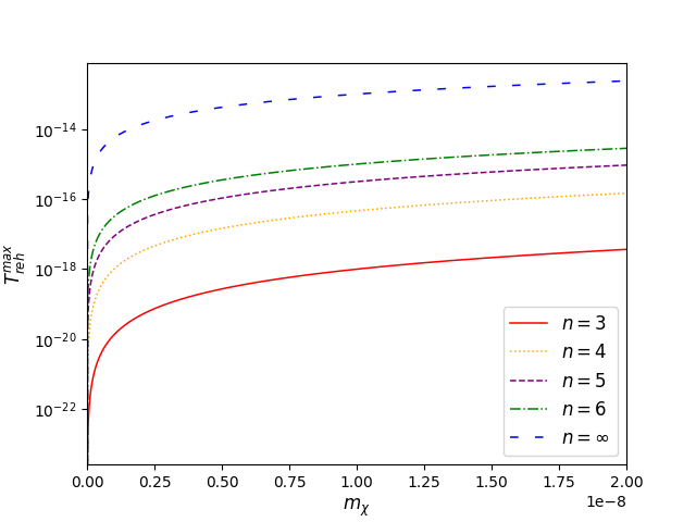
Figure 1: We show the nature of $T_{\rm max}^{\rm reh}$ influenced by the mass of the produced particles, $m_{\chi}$, for different values of $n$, considering the units where $M_{\rm pl}=1$.

An important final remark is in order: Since the maximum reheating temperature only depends on the mass of produced particles, one has a direct relationship between that mass and the spectral index. And recalling that for the range of viable masses (84), the maximum reheating temperature is lower than $10^{9}$ GeV, we can better constraint the spectral index, as we show in Table 4.

$n$	$n_{s}$	${T_{\rm reh}^{\rm max}}/{M_{\rm pl}}$
$3$	$0.9677\leq n_{s}\leq 0.9683$	${T_{\rm reh}^{\rm max}}/{M_{\rm pl}}\leq 2\times 10^{-15}$
$4$	$0.9678\leq n_{s}\leq 0.9693$	${T_{\rm reh}^{\rm max}}/{M_{\rm pl}}\leq 3\times 10^{-14}$
$5$	$0.9679\leq n_{s}\leq 0.9699$	${T_{\rm reh}^{\rm max}}/{M_{\rm pl}}\leq 10^{-13}$
$6$	$0.9681\leq n_{s}\leq 0.9702$	${T_{\rm reh}^{\rm max}}/{M_{\rm pl}}\leq 3\times 10^{-13}$
$\infty$	$0.9684\leq n_{s}\leq 0.9719$	${T_{\rm reh}^{\rm max}}/{M_{\rm pl}}\leq 7\times 10^{-12}$

Table 4: Range of viable values of the spectral index when one considers the maximum reheating temperature.

V Gravitational dark matter production

In this section, we study the gravitational production of dark matter within the context of gravitational reheating. Specifically, we consider two quantum scalar fields, $X$ and $Y$. The $X$-field is responsible for the gravitational production of $X$-particles with mass $m_{X}$, which will decay into SM particles to reheat the universe. The $Y$-field, on the other hand, is responsible for the production of $Y$-particles with mass $m_{Y}$, which will account for present-day dark matter.

Assuming that the decay of the $X$-particles occurs during the inflaton domination. At the onset of radiation the energy density of the $X$-particles is (59):

$$\langle\rho_{X,\rm reh}\rangle\cong 3H_{\rm END}^{2}M_{\rm pl}^{2}\left(\frac{H_{\rm END}}{\Gamma_{X}}\right)^{\frac{n+1}{n-2}}\Theta_{X}^{\frac{3n}{n-2}},$$ (85)

where $\Gamma_{X}$ is the decay rate of the $X$-particles and $\Theta_{X}$ the heating efficiency corresponding to the $X$-particles.

At the matter-radiation equality, which we will denote by ”eq”, we will have:

$$\frac{a_{\rm reh}}{a_{\rm eq}}=\frac{\langle\rho_{Y,\rm reh}\rangle}{\langle\rho_{X,\rm reh}\rangle}\Longrightarrow\langle\rho_{Y,\rm eq}\rangle=\frac{\langle\rho_{Y,\rm reh}\rangle^{4}}{\langle\rho_{X,\rm reh}\rangle^{3}}.$$ (86)

Next, we have to take into account that

$$\langle\rho_{Y,\rm reh}\rangle=\langle\rho_{Y,\rm END}\rangle\left(\frac{a_{\rm END}}{a_{\rm reh}}\right)^{3}$$

$$=3H_{\rm END}^{2}M_{\rm pl}^{2}\left(\frac{H_{\rm END}}{\Gamma_{X}}\right)^{\frac{(n+1)^{2}}{2n(n-2)}}\Theta_{X}^{\frac{3(n+1)}{2(n-2)}}\Theta_{Y},$$ (87)

where we have used the relation (58):

$$\Theta_{X}=\left(\frac{\Gamma_{X}}{H_{\rm END}}\right)^{\frac{n+1}{3n}}\left(\frac{a_{\rm END}}{a_{\rm reh}}\right)^{\frac{2(n-2)}{n+1}}.$$ (88)

Therefore:

$$\langle\rho_{Y,\rm eq}\rangle=3H_{\rm END}^{2}M_{\rm pl}^{2}\left(\frac{H_{\rm END}}{\Gamma_{X}}\right)^{-\frac{n+1}{n}}\Theta_{X}^{-3}\Theta_{Y}^{4}.$$ (89)

On the other hand, considering the central values of the red shift at the matter-radiation equality $z_{\rm eq}=3365$, the present value of the ratio of the matter energy density to the critical one is $\Omega_{\rm m,0}=0.308$, and $H_{0}=67.81$ Km/sec/Mpc, one can deduce that the present value of the matter energy density is $\rho_{\rm m,0}=3H^{2}_{0}M^{2}_{\rm pl}\Omega_{\rm m,0}\cong 3\times 10^{-121}M^{4}_{\rm pl}$, and at matter radiation equality one will have $\rho_{\rm m,\rm eq}=\rho_{\rm m,0}(1+z_{\rm eq})^{3}\cong 10^{-110}M_{\rm pl}^{4}$. Since practically all the matter has a not baryonic origin, one can conclude that $\langle\rho_{Y,\rm eq}\rangle\cong\rho_{\rm m,\rm eq}$, and thus, we have the relation between the decay rate of the $X$-particles and the heating efficiencies.

Then,

$$\frac{\Gamma_{X}}{H_{\rm END}}\cong\left(\frac{\Theta_{X}^{3}}{12\Theta_{Y}^{4}}\right)^{\frac{n}{n+1}}10^{-\frac{98n}{n+1}},$$ (90)

where we have used that $H_{\rm END}\cong 2\times 10^{-6}M_{\rm pl}$, and from the constraint (65), we get:

$$10^{99}\left(\frac{m_{X}}{M_{\rm pl}}\right)^{\frac{5(n+1)}{2(n-1)}}\ll\frac{\Theta_{X}^{3}}{\Theta_{Y}^{4}}\lesssim 5\times 10^{\frac{2(85n-72)}{n}}\left(\frac{m_{X}}{M_{\rm pl}}\right)^{\frac{15}{2}}.$$ (91)

Next, from (56), we have $\Theta_{A}\cong{1.5}\left(\frac{m_{A}}{M_{\rm pl}}\right)^{5/2}$, with $A=X,Y$, which leads to the following relation between the masses:

$$8\times 10^{-18}\times 10^{\frac{72}{5n}}\lesssim\frac{m_{Y}}{M_{\rm pl}}\ll 10^{-10}\left(\frac{m_{X}}{M_{\rm pl}}\right)^{\frac{n-2}{2(n-1)}}.$$ (92)

In Table 5 we present the range of viable masses for different values of $n$.

$n$	$m_{X}/M_{\rm pl}$	$m_{Y}/M_{\rm pl}$
$3$	$3\times 10^{-9}\ll{m_{X}}/{M_{\rm pl}}\ll 4\times 10^{-7}\quad$	$6\times 10^{-13}\lesssim{m_{Y}}/{M_{\rm pl}}\ll 10^{-10}\left(\frac{m_{X}}{M_{\rm pl}}\right)^{1/4}$
$4$	$9\times 10^{-11}\leq{m_{\chi}}/{M_{\rm pl}}\ll 6\times 10^{-8}$	$4\times 10^{-14}\lesssim{m_{Y}}/{M_{\rm pl}}\ll 10^{-10}\left(\frac{m_{X}}{M_{\rm pl}}\right)^{1/3}$
$5$	$2\times 10^{-11}\leq{m_{\chi}}/{M_{\rm pl}}\ll 2\times 10^{-8}$	$7\times 10^{-15}\lesssim{m_{Y}}/{M_{\rm pl}}\ll 10^{-10}\left(\frac{m_{X}}{M_{\rm pl}}\right)^{3/8}$
$6$	$6\times 10^{-12}\leq{m_{\chi}}/{M_{\rm pl}}\ll 9\times 10^{-9}$	$2\times 10^{-15}\lesssim{m_{Y}}/{M_{\rm pl}}\ll 10^{-10}\left(\frac{m_{X}}{M_{\rm pl}}\right)^{2/5}$
$\infty$	$3\times 10^{-14}\ll{m_{\chi}}/{M_{\rm pl}}\ll 2\times 10^{-10}$	$10^{-17}\lesssim{m_{Y}}/{M_{\rm pl}}\ll 10^{-10}\left(\frac{m_{X}}{M_{\rm pl}}\right)^{1/2}$

Table 5: Range of viable $X$ and $Y$ masses.

$n$	$\frac{m_{Y}}{M_{\rm pl}}$
$3$	$\frac{m_{Y}}{M_{\rm pl}}\cong 10^{-10}\left(\frac{m_{X}}{M_{\rm pl}}\right)^{\frac{1}{4}}\Longrightarrow 7\times 10^{-13}\leq\frac{m_{Y}}{M_{\rm pl}}\ll 4\times 10^{-12}$
$4$	$\frac{m_{Y}}{M_{\rm pl}}\cong 10^{-10}\left(\frac{m_{X}}{M_{\rm pl}}\right)^{\frac{1}{3}}\Longrightarrow 4\times 10^{-14}\leq\frac{m_{Y}}{M_{\rm pl}}\ll 10^{-12}$
$5$	$\frac{m_{Y}}{M_{\rm pl}}\cong 10^{-10}\left(\frac{m_{X}}{M_{\rm pl}}\right)^{\frac{3}{8}}\Longrightarrow 9\times 10^{-15}\leq\frac{m_{Y}}{M_{\rm pl}}\ll 7\times 10^{-13}$
$6$	$\frac{m_{Y}}{M_{\rm pl}}\cong 10^{-10}\left(\frac{m_{X}}{M_{\rm pl}}\right)^{\frac{2}{5}}\Longrightarrow 3\times 10^{-15}\leq\frac{m_{Y}}{M_{\rm pl}}\ll 5\times 10^{-13}$
$\infty$	$\frac{m_{Y}}{M_{\rm pl}}\cong 10^{-10}\left(\frac{m_{X}}{M_{\rm pl}}\right)^{\frac{1}{2}}\Longrightarrow 2\times 10^{-17}\leq\frac{m_{Y}}{M_{\rm pl}}\ll 10^{-13}$

Table 6: Range of viable masses for the dark matter.

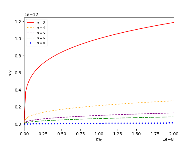
Figure 2: Plot of $m_{Y}$ masses as a function of $m_{X}$. For: $n=3$ red, $n=4$ orange, $n=5$ purple, $n=6$ green and $n=\infty$ blue. In the plot the units are $M_{\rm pl}=1$.

V.1 Dark matter production when the reheating temperature is maximum

As we have already shown, the reheating temperature attains its maximum value when the decay occurs close to the end of the inflaton’s domination. In this situation, the energy density of the $X$-field at the onset of radiation epoch is $\langle\rho_{X,\rm reh}\rangle=3H_{\rm END}^{2}M_{\rm pl}^{2}\Theta_{X}^{\frac{2n}{n-1}}$ and the one o the $Y$-field is $\langle\rho_{Y,\rm reh}\rangle=3H_{\rm END}^{2}M_{\rm pl}^{2}\Theta_{X}^{\frac{n+1}{n-1}}\Theta_{Y}$, which leads to

$$\langle\rho_{Y,\rm eq}\rangle=3H_{\rm END}^{2}M_{\rm pl}^{2}\Theta_{X}^{-\frac{2(n-2)}{n-1}}\Theta_{Y}^{4}.$$ (93)

And thus,

$$3\frac{H_{\rm END}^{2}}{M_{\rm pl}^{2}}\Theta_{X}^{-\frac{2(n-2)}{n-1}}\Theta_{Y}^{4}\cong 10^{-110}$$

$$\Longrightarrow 12\Theta_{X}^{-\frac{2(n-2)}{n-1}}\Theta_{Y}^{4}\cong 10^{-98}.$$ (94)

What leads to the following link between both masses

$$\frac{m_{Y}}{M_{\rm pl}}\cong 10^{-10}\left(\frac{m_{X}}{M_{\rm pl}}\right)^{\frac{n-2}{2(n-1)}},$$ (95)

and thus, as we have already explained, since the mass of the particles responsible for the reheating in relation with the spectral index, one concludes that the mass of dark matter, when one assumes that the onset of radiation is close to the decay of $X$-particles obtaining the maximum reheating temperature, is related by the spectral index via the formulas (84) and (95) and (III.1)

Finally, taking into account the range of values obtained for the masses $m_{X}$ (summarized in Table 3), we show in Table 6 the range of the values of the masses $m_{Y}$ for different values of the parameter $n$ and in Figure  2 we show the graphical relation between $m_{X}$ and $m_{Y}$ for different values of $n$.

VI Conclusions

In this article, we examine gravitational reheating as a result of massive particle production when a massive scalar quantum field is conformally coupled to the Ricci scalar. In this framework, calculating the energy density of particles produced at the end of inflation—considering that the number of final $e$-folds establishes a relationship between the spectral index of scalar perturbations and the reheating temperature enables us, after obtaining the formula of the reheating temperature, to link the spectral index to the mass of the generated particles. Assuming a feasible reheating temperature, consistent with Big Bang Nucleosynthesis and avoiding issues related to the gravitino problem, we can place constraints on the possible masses of these particles, and consequently on the spectral index.

Furthermore, we explore the gravitational production of dark matter, deriving relationships between the mass of the particles responsible for reheating and the mass of dark matter particles. These connections provide a natural linkage between the reheating process and the origin of dark matter, offering constraints that enhance our understanding of both early-universe dynamics and dark matter genesis within a gravitational reheating scenario.

Our results indicate that, in the framework of gravitational particle production, the relationship between the mass of reheating particles and the dark matter mass can yield insights into viable particle mass ranges that comply with observational constraints on the spectral index and reheating temperature. This approach not only strengthens the theoretical basis for gravitational reheating but also aligns with existing cosmological models that incorporate gravitational dark matter production. Thus, by establishing mass bounds, this study contributes to a more precise picture of the mechanisms at play during the transition from inflation to the reheated universe, connecting fundamental aspects of inflationary theory with dark matter production pathways.

References

- Guth (1981) Alan H. Guth, “The Inflationary Universe: A Possible Solution to the Horizon and Flatness Problems,” Phys. Rev. D 23, 347–356 (1981).
- Linde (1982) Andrei D. Linde, “A New Inflationary Universe Scenario: A Possible Solution of the Horizon, Flatness, Homogeneity, Isotropy and Primordial Monopole Problems,” Phys. Lett. B 108, 389–393 (1982).
- Barrow and Turner (1981) John D. Barrow and Michael S. Turner, “Inflation in the Universe,” Nature 292, 35–38 (1981).
- Spokoiny (1984) B. L. Spokoiny, “INFLATION AND GENERATION OF PERTURBATIONS IN BROKEN SYMMETRIC THEORY OF GRAVITY,” Phys. Lett. B 147, 39–43 (1984).
- Steinhardt and Turner (1984) P. J. Steinhardt and Michael S. Turner, “A Prescription for Successful New Inflation,” Phys. Rev. D 29, 2162–2171 (1984).
- Lucchin and Matarrese (1985) F. Lucchin and S. Matarrese, “Power Law Inflation,” Phys. Rev. D 32, 1316 (1985).
- Hawking (1985) S. W. Hawking, “Limits on Inflationary Models of the Universe,” Phys. Lett. B 150, 339–341 (1985).
- Lyth (1985) D. H. Lyth, “Large Scale Energy Density Perturbations and Inflation,” Phys. Rev. D 31, 1792–1798 (1985).
- Belinsky et al. (1985) V. A. Belinsky, I. M. Khalatnikov, L. P. Grishchuk, and Ya. B. Zeldovich, “Inflationary stages in cosmological models with a scalar field,” Phys. Lett. B 155, 232–236 (1985).
- Mijic et al. (1986) Milan B. Mijic, Michael S. Morris, and Wai-Mo Suen, “The R**2 Cosmology: Inflation Without a Phase Transition,” Phys. Rev. D 34, 2934 (1986).
- Khalfin (1986) L. A. Khalfin, “Bounds on inflationary models of the universe,” Sov. Phys. JETP 64, 673–676 (1986).
- Silk and Turner (1987) Joseph Silk and Michael S. Turner, “Double Inflation,” Phys. Rev. D 35, 419 (1987).
- Burd and Barrow (1988) A. B. Burd and John D. Barrow, “Inflationary Models with Exponential Potentials,” Nucl. Phys. B 308, 929–945 (1988), [Erratum: Nucl.Phys.B 324, 276–276 (1989)].
- Olive (1990) Keith A. Olive, “Inflation,” Phys. Rept. 190, 307–403 (1990).
- Ford (1989) L. H. Ford, “Inflation Driven by a Vector Field,” Phys. Rev. D 40, 967 (1989).
- Adams et al. (1991) Fred C. Adams, Katherine Freese, and Alan H. Guth, “Constraints on the scalar field potential in inflationary models,” Phys. Rev. D 43, 965–976 (1991).
- Freese et al. (1990) Katherine Freese, Joshua A. Frieman, and Angela V. Olinto, “Natural inflation with pseudo - Nambu-Goldstone bosons,” Phys. Rev. Lett. 65, 3233–3236 (1990).
- Wang (1991) Yun Wang, “Constraints on generalized extended inflationary models,” Phys. Rev. D 44, 991–998 (1991).
- Polarski and Starobinsky (1992) David Polarski and Alexei A. Starobinsky, “Spectra of perturbations produced by double inflation with an intermediate matter dominated stage,” Nucl. Phys. B 385, 623–650 (1992).
- Liddle and Lyth (1992) Andrew R. Liddle and David H. Lyth, “COBE, gravitational waves, inflation and extended inflation,” Phys. Lett. B 291, 391–398 (1992), arXiv:astro-ph/9208007 .
- Linde (1994) Andrei D. Linde, “Hybrid inflation,” Phys. Rev. D 49, 748–754 (1994), arXiv:astro-ph/9307002 .
- Barrow (1993) John D. Barrow, “New types of inflationary universe,” Phys. Rev. D 48, 1585–1590 (1993).
- Barrow (1994) John D. Barrow, “Exact inflationary universes with potential minima,” Phys. Rev. D 49, 3055–3058 (1994).
- Vilenkin (1994) Alexander Vilenkin, “Topological inflation,” Phys. Rev. Lett. 72, 3137–3140 (1994), arXiv:hep-th/9402085 .
- Peter et al. (1994) Patrick Peter, David Polarski, and Alexei A. Starobinsky, “Confrontation of double inflationary models with observations,” Phys. Rev. D 50, 4827–4834 (1994), arXiv:astro-ph/9403037 .
- Sasaki and Stewart (1996) Misao Sasaki and Ewan D. Stewart, “A General analytic formula for the spectral index of the density perturbations produced during inflation,” Prog. Theor. Phys. 95, 71–78 (1996), arXiv:astro-ph/9507001 .
- Barrow and Parsons (1995) John D. Barrow and Paul Parsons, “Inflationary models with logarithmic potentials,” Phys. Rev. D 52, 5576–5587 (1995), arXiv:astro-ph/9506049 .
- Lidsey et al. (1997) James E. Lidsey, Andrew R. Liddle, Edward W. Kolb, Edmund J. Copeland, Tiago Barreiro, and Mark Abney, “Reconstructing the inflation potential : An overview,” Rev. Mod. Phys. 69, 373–410 (1997), arXiv:astro-ph/9508078 .
- Parsons and Barrow (1995) Paul Parsons and John D. Barrow, “Generalized scalar field potentials and inflation,” Phys. Rev. D 51, 6757–6763 (1995), arXiv:astro-ph/9501086 .
- Liddle (1998) Andrew R. Liddle, “Inflation and the cosmic microwave background,” Phys. Rept. 307, 53–60 (1998), arXiv:astro-ph/9801148 .
- Guth (2000) Alan H. Guth, “Inflation and eternal inflation,” Phys. Rept. 333, 555–574 (2000), arXiv:astro-ph/0002156 .
- Riotto (2003) Antonio Riotto, “Inflation and the theory of cosmological perturbations,” ICTP Lect. Notes Ser. 14, 317–413 (2003), arXiv:hep-ph/0210162 .
- Feinstein (2002) Alexander Feinstein, “Power law inflation from the rolling tachyon,” Phys. Rev. D 66, 063511 (2002), arXiv:hep-th/0204140 .
- Ashcroft et al. (2004) P. R. Ashcroft, C. van de Bruck, and A. C. Davis, “Inflationary dynamics with runaway potentials,” Phys. Rev. D 69, 083516 (2004), arXiv:astro-ph/0210597 .
- Boubekeur and Lyth (2005) Lotfi Boubekeur and David. H. Lyth, “Hilltop inflation,” JCAP 07, 010 (2005), arXiv:hep-ph/0502047 .
- Conlon and Quevedo (2006) Joseph P. Conlon and Fernando Quevedo, “Kahler moduli inflation,” JHEP 01, 146 (2006), arXiv:hep-th/0509012 .
- Ferraro and Fiorini (2007) Rafael Ferraro and Franco Fiorini, “Modified teleparallel gravity: Inflation without inflaton,” Phys. Rev. D 75, 084031 (2007), arXiv:gr-qc/0610067 .
- Cheung et al. (2008) Clifford Cheung, Paolo Creminelli, A. Liam Fitzpatrick, Jared Kaplan, and Leonardo Senatore, “The Effective Field Theory of Inflation,” JHEP 03, 014 (2008), arXiv:0709.0293 [hep-th] .
- Chen et al. (2008) Xingang Chen, Richard Easther, and Eugene A. Lim, “Generation and Characterization of Large Non-Gaussianities in Single Field Inflation,” JCAP 04, 010 (2008), arXiv:0801.3295 [astro-ph] .
- Baumann and Peiris (2009) Daniel Baumann and Hiranya V. Peiris, “Cosmological Inflation: Theory and Observations,” Adv. Sci. Lett. 2, 105–120 (2009), arXiv:0810.3022 [astro-ph] .
- Koivisto and Mota (2008) Tomi Koivisto and David F. Mota, “Vector Field Models of Inflation and Dark Energy,” JCAP 08, 021 (2008), arXiv:0805.4229 [astro-ph] .
- Pal et al. (2010) Barun Kumar Pal, Supratik Pal, and B. Basu, “Mutated Hilltop Inflation : A Natural Choice for Early Universe,” JCAP 01, 029 (2010), arXiv:0908.2302 [hep-th] .
- Martin et al. (2014a) Jérôme Martin, Christophe Ringeval, Roberto Trotta, and Vincent Vennin, “The Best Inflationary Models After Planck,” JCAP 03, 039 (2014a), arXiv:1312.3529 [astro-ph.CO] .
- Martin et al. (2014b) Jerome Martin, Christophe Ringeval, and Vincent Vennin, “Encyclopædia Inflationaris,” Phys. Dark Univ. 5-6, 75–235 (2014b), arXiv:1303.3787 [astro-ph.CO] .
- Sebastiani et al. (2014) L. Sebastiani, G. Cognola, R. Myrzakulov, S. D. Odintsov, and S. Zerbini, “Nearly Starobinsky inflation from modified gravity,” Phys. Rev. D 89, 023518 (2014), arXiv:1311.0744 [gr-qc] .
- Hamada et al. (2014) Yuta Hamada, Hikaru Kawai, Kin-ya Oda, and Seong Chan Park, “Higgs Inflation is Still Alive after the Results from BICEP2,” Phys. Rev. Lett. 112, 241301 (2014), arXiv:1403.5043 [hep-ph] .
- Freese and Kinney (2015) Katherine Freese and William H. Kinney, “Natural Inflation: Consistency with Cosmic Microwave Background Observations of Planck and BICEP2,” JCAP 03, 044 (2015), arXiv:1403.5277 [astro-ph.CO] .
- van de Bruck and Paduraru (2015) Carsten van de Bruck and Laura Elena Paduraru, “Simplest extension of Starobinsky inflation,” Phys. Rev. D 92, 083513 (2015), arXiv:1505.01727 [hep-th] .
- van de Bruck and Longden (2016a) Carsten van de Bruck and Chris Longden, “Higgs Inflation with a Gauss-Bonnet term in the Jordan Frame,” Phys. Rev. D 93, 063519 (2016a), arXiv:1512.04768 [hep-ph] .
- van de Bruck and Longden (2016b) Carsten van de Bruck and Chris Longden, “Running of the Running and Entropy Perturbations During Inflation,” Phys. Rev. D 94, 021301 (2016b), arXiv:1606.02176 [astro-ph.CO] .
- Ratra (2017) Bharat Ratra, “Inflation in a closed universe,” Phys. Rev. D 96, 103534 (2017), arXiv:1707.03439 [astro-ph.CO] .
- Rubio (2019) Javier Rubio, “Higgs inflation,” Front. Astron. Space Sci. 5, 50 (2019), arXiv:1807.02376 [hep-ph] .
- Giarè et al. (2019) William Giarè, Eleonora Di Valentino, and Alessandro Melchiorri, “Testing the inflationary slow-roll condition with tensor modes,” Phys. Rev. D 99, 123522 (2019).
- van de Bruck and Daniel (2021) Carsten van de Bruck and Richard Daniel, “Inflation and scale-invariant R2 gravity,” Phys. Rev. D 103, 123506 (2021), arXiv:2102.11719 [gr-qc] .
- Forconi et al. (2021) Matteo Forconi, William Giarè, Eleonora Di Valentino, and Alessandro Melchiorri, “Cosmological constraints on slow roll inflation: An update,” Phys. Rev. D 104, 103528 (2021), arXiv:2110.01695 [astro-ph.CO] .
- Odintsov et al. (2023) Sergei D. Odintsov, Vasilis K. Oikonomou, Ifigeneia Giannakoudi, Fotis P. Fronimos, and Eirini C. Lymperiadou, “Recent Advances in Inflation,” Symmetry 15, 1701 (2023), arXiv:2307.16308 [gr-qc] .
- Giarè et al. (2023) William Giarè, Supriya Pan, Eleonora Di Valentino, Weiqiang Yang, Jaume de Haro, and Alessandro Melchiorri, “Inflationary potential as seen from different angles: model compatibility from multiple CMB missions,” JCAP 09, 019 (2023), arXiv:2305.15378 [astro-ph.CO] .
- Jinno et al. (2024) Ryusuke Jinno, Kazunori Kohri, Takeo Moroi, Tomo Takahashi, and Masashi Hazumi, “Testing multi-field inflation with LiteBIRD,” JCAP 03, 011 (2024), arXiv:2310.08158 [astro-ph.CO] .
- Garfinkle et al. (2023) David Garfinkle, Anna Ijjas, and Paul J. Steinhardt, “Initial conditions problem in cosmological inflation revisited,” Phys. Lett. B 843, 138028 (2023), arXiv:2304.12150 [gr-qc] .
- Akrami et al. (2020) Y. Akrami et al. (Planck), “Planck 2018 results. X. Constraints on inflation,” Astron. Astrophys. 641, A10 (2020), arXiv:1807.06211 [astro-ph.CO] .
- de Haro et al. (2024) Jaume de Haro, Llibert Aresté Saló, and Supriya Pan, “Gravitational reheating formulas and bounds in oscillating backgrounds,” (to appear in Phys. Rev. D); 2411.01671 (2024).
- Zeldovich and Starobinsky (1971) Ya. B. Zeldovich and Alexei A. Starobinsky, “Particle production and vacuum polarization in an anisotropic gravitational field,” Zh. Eksp. Teor. Fiz. 61, 2161–2175 (1971).
- Bogolyubov (1958) N. N. Bogolyubov, “On a New method in the theory of superconductivity,” Nuovo Cim. 7, 794–805 (1958).
- Drewes et al. (2017) Marco Drewes, Jin U Kang, and Ui Ri Mun, “CMB constraints on the inflaton couplings and reheating temperature in -attractor inflation,” JHEP 11, 072 (2017), arXiv:1708.01197 [astro-ph.CO] .
- Turner (1983) Michael S. Turner, “Coherent Scalar Field Oscillations in an Expanding Universe,” Phys. Rev. D 28, 1243 (1983).
- Garcia et al. (2021) Marcos A. G. Garcia, Kunio Kaneta, Yann Mambrini, and Keith A. Olive, “Inflaton Oscillations and Post-Inflationary Reheating,” JCAP 04, 012 (2021), arXiv:2012.10756 [hep-ph] .
- Kaneta et al. (2022) Kunio Kaneta, Sung Mook Lee, and Kin-ya Oda, “Boltzmann or Bogoliubov? Approaches compared in gravitational particle production,” JCAP 09, 018 (2022), arXiv:2206.10929 [astro-ph.CO] .
- Ford (1987) L. H. Ford, “Gravitational Particle Creation and Inflation,” Phys. Rev. D 35, 2955 (1987).
- Chun et al. (2009) E. J. Chun, S. Scopel, and I. Zaballa, “Gravitational reheating in quintessential inflation,” JCAP 07, 022 (2009), arXiv:0904.0675 [hep-ph] .
- Lankinen and Vilja (2017) Juho Lankinen and Iiro Vilja, “Gravitational Particle Creation in a Stiff Matter Dominated Universe,” JCAP 08, 025 (2017), arXiv:1612.02586 [gr-qc] .
- Haro et al. (2019) Jaume Haro, Weiqiang Yang, and Supriya Pan, “Reheating in quintessential inflation via gravitational production of heavy massive particles: A detailed analysis,” JCAP 01, 023 (2019), arXiv:1811.07371 [gr-qc] .
- Jenks et al. (2024) Leah Jenks, Edward W. Kolb, and Keyer Thyme, “Gravitational Particle Production of Scalars: Analytic and Numerical Approaches Including Early Reheating,” (2024), arXiv:2410.03938 [hep-ph] .
- Ema et al. (2018) Yohei Ema, Kazunori Nakayama, and Yong Tang, “Production of Purely Gravitational Dark Matter,” JHEP 09, 135 (2018), arXiv:1804.07471 [hep-ph] .
- Chung et al. (2001) Daniel J. H. Chung, Patrick Crotty, Edward W. Kolb, and Antonio Riotto, “On the Gravitational Production of Superheavy Dark Matter,” Phys. Rev. D 64, 043503 (2001), arXiv:hep-ph/0104100 .
- Garcia et al. (2020) Marcos A. G. Garcia, Kunio Kaneta, Yann Mambrini, and Keith A. Olive, “Reheating and Post-inflationary Production of Dark Matter,” Phys. Rev. D 101, 123507 (2020), arXiv:2004.08404 [hep-ph] .
- Hashiba and Yokoyama (2019) Soichiro Hashiba and Jun’ichi Yokoyama, “Gravitational reheating through conformally coupled superheavy scalar particles,” JCAP 01, 028 (2019), arXiv:1809.05410 [gr-qc] .
- Hashiba and Yamada (2021) Soichiro Hashiba and Yusuke Yamada, “Stokes phenomenon and gravitational particle production — How to evaluate it in practice,” JCAP 05, 022 (2021), arXiv:2101.07634 [hep-th] .
- Landau and Lifshitz (1991) L.D. Landau and E.M. Lifshitz, Quantum Mechanics: Non-Relativistic Theory, Course of theoretical physics (Elsevier Science, 1991).
- Abramowitz and Stegun (1965) M. Abramowitz and I.A. Stegun, Handbook of Mathematical Functions: With Formulas, Graphs, and Mathematical Tables, Applied mathematics series (Dover Publications, 1965).
- Chung (2003) Daniel J. H. Chung, “Classical Inflation Field Induced Creation of Superheavy Dark Matter,” Phys. Rev. D 67, 083514 (2003), arXiv:hep-ph/9809489 .
- Rehagen and Gelmini (2015) Thomas Rehagen and Graciela B. Gelmini, “Low reheating temperatures in monomial and binomial inflationary potentials,” JCAP 06, 039 (2015), arXiv:1504.03768 [hep-ph] .
- Ellis et al. (1982) John R. Ellis, Andrei D. Linde, and Dimitri V. Nanopoulos, “Inflation Can Save the Gravitino,” Phys. Lett. B 118, 59–64 (1982).
- Khlopov and Linde (1984) M. Yu. Khlopov and Andrei D. Linde, “Is It Easy to Save the Gravitino?” Phys. Lett. B 138, 265–268 (1984).
- Felder et al. (1999) Gary N. Felder, Lev Kofman, and Andrei D. Linde, “Inflation and preheating in NO models,” Phys. Rev. D 60, 103505 (1999), arXiv:hep-ph/9903350 .
- Rubio and Wetterich (2017) Javier Rubio and Christof Wetterich, “Emergent scale symmetry: Connecting inflation and dark energy,” Phys. Rev. D 96, 063509 (2017), arXiv:1705.00552 [gr-qc] .
- Kawasaki et al. (2005) Masahiro Kawasaki, Kazunori Kohri, and Takeo Moroi, “Big-Bang nucleosynthesis and hadronic decay of long-lived massive particles,” Phys. Rev. D 71, 083502 (2005), arXiv:astro-ph/0408426 .
- Kawasaki et al. (2006) Masahiro Kawasaki, Fuminobu Takahashi, and T. T. Yanagida, “The Gravitino-overproduction problem in inflationary universe,” Phys. Rev. D 74, 043519 (2006), arXiv:hep-ph/0605297 .
- Kawasaki et al. (2018) Masahiro Kawasaki, Kazunori Kohri, Takeo Moroi, and Yoshitaro Takaesu, “Revisiting Big-Bang Nucleosynthesis Constraints on Long-Lived Decaying Particles,” Phys. Rev. D 97, 023502 (2018), arXiv:1709.01211 [hep-ph] .
- Davidson et al. (2000) Sacha Davidson, Marta Losada, and Antonio Riotto, “A New perspective on baryogenesis,” Phys. Rev. Lett. 84, 4284–4287 (2000), arXiv:hep-ph/0001301 .
- Peebles and Vilenkin (1999) P. J. E. Peebles and A. Vilenkin, “Quintessential inflation,” Phys. Rev. D 59, 063505 (1999), arXiv:astro-ph/9810509 .
- Giovannini (1998) Massimo Giovannini, “Gravitational waves constraints on postinflationary phases stiffer than radiation,” Phys. Rev. D 58, 083504 (1998), arXiv:hep-ph/9806329 .
- Aghanim et al. (2020) N. Aghanim et al. (Planck), “Planck 2018 results. VI. Cosmological parameters,” Astron. Astrophys. 641, A6 (2020), [Erratum: Astron.Astrophys. 652, C4 (2021)], arXiv:1807.06209 [astro-ph.CO] .