The thermodynamic profile of AdS black holes in Lorentz invariance-violating Bumblebee and Kalb-Ramond gravity

Abstract

Lorentz invariance violation (LIV) is a topic of significant interest in quantum gravity and in extensions of the Standard Model of particle physics. Recently, new classes of black hole solutions have been proposed, involving vector fields and rank-two antisymmetric tensor fields that acquire nontrivial vacuum expectation values, resulting in the Bumblebee and Kalb-Ramond (KR) gravity models, respectively. These models exhibit novel geometric structures and differ in notable ways from standard Einstein gravity. In this study, we examine neutral anti-de Sitter (AdS) black holes within the context of LIV backgrounds, focusing on their thermodynamic properties through two distinct approaches. The first approach utilizes the free energy landscape framework, revealing substantial modifications to the conventional Hawking-Page phase transition. Specifically, LIV effects can alter the stability regimes of black holes and thermal AdS phases, potentially leading to overlapping thermodynamic regimes that would otherwise remain distinct. This suggests that LIV introduces complex modifications to the phase behavior of black holes, offering new insights into their stability characteristics. The second approach involves thermodynamic Ruppeiner geometry, which provides a window into the microstructure of black holes via a well-defined scalar curvature. In general, LIV effects are negligible for larger black holes, which behave like an ideal gas with no significant interactions among their constituents. However, at shorter length scales, the presence of LIV can induce multiple stable and unstable phase transitions, depending on the specific gravity model and the magnitude of LIV effects considered. Finally, we analyze particle emission rates associated with Hawking evaporation in these models. While Bumblebee and Kalb-Ramond gravity share several similarities, we identify distinctive signatures arising from their underlying physical mechanisms. These differences may provide key observational and theoretical constraints for testing LIV effects in black hole physics.

I Introduction

Central to the foundations of modern physics, Lorentz symmetry posits the equivalence of physical laws across all inertial frames. Its testable aspects have consistently demonstrated it to be a fundamental symmetry governing physical phenomena in the Universe Mariz et al. (2023); Tasson (2014). However, recent advancements in various domains of physics have indicated potential violations of this symmetry. Notable examples include string theory Kostelecky and Samuel (1989a); Bluhm and Kostelecky (2005), loop quantum gravity Alfaro et al. (2002); Gambini and Pullin (1999), noncommutative field theory Carroll et al. (2001), massive gravity Dubovsky et al. (2005), Einstein-Aether theory Jacobson and Mattingly (2001), and Hořava-Lifshitz gravity Horava (2009). Such findings have significant implications for our understanding of fundamental physics. These efforts can be viewed as part of the ongoing endeavor to unify gravity with quantum field theory and particle physics, encapsulated in the effective field theory known as the Standard Model Extension (SME) Liberati (2013). Within this framework, it is commonly posited that potential signatures of Lorentz invariance violation (LIV) may emerge near the Planck scale Kostelecky (2004), providing a promising avenue for the pursuit of a consistent theory of quantum gravity. Some of the earliest efforts to comprehend the electromagnetic sector of the SME are documented in the literature Colladay and Kostelecky (2001); Kostelecky and Lehnert (2001); Kostelecky and Lane (1999); Yoder and Adkins (2012). Similarly, investigations into the electroweak Colladay and McDonald (2009); Mouchrek-Santos and Ferreira (2017) and strong interactions Abazov et al. (2012); Berger et al. (2016) within the SME framework have also gained traction in recent years. Furthermore, significant efforts have been devoted to understanding the gravitational aspects of the SME Bluhm and Kostelecky (2005); Bailey (2009); Tso and Bailey (2011); Maluf et al. (2013); Bluhm et al. (2008a); Bailey and Kostelecky (2006). In addition to this theoretical framework, experimental and observational investigations into Lorentz violation are also being pursued Amelino-Camelia et al. (1998); Mattingly (2005); Tasson (2014); Addazi et al. (2022); Piran and Ofengeim (2024); Cao et al. (2024).
Nontrivial LIV can arise in either an explicit or spontaneous manner. Explicit violation occurs when the Lagrangian density of a theory lacks Lorentz symmetry, resulting in physical laws that take different forms in different reference frames. In contrast, spontaneous violation of Lorentz symmetry arises when the Lagrangian density retains Lorentz symmetry, yet the ground state of the physical system does not Kostelecky (2004). Our focus here is on spontaneous symmetry breaking, which can occur for various reasons. A notable example involves a vector field acquiring a nonzero vacuum expectation value (VEV), resulting in a preferred directionality in spacetime and thus spontaneously breaking local Lorentz invariance for particles. These entities are referred to as Bumblebee fields, and the associated framework within the gravitational sector is commonly known as Bumblebee gravity Kostelecky and Samuel (1989b, c); Bailey and Kostelecky (2006); Bluhm et al. (2008b). Over the past decade, Bumblebee gravity has assumed a prominent role in black hole physics. Casana et al. Casana et al. (2018) proposed a solution for a spherically symmetric black hole within the framework of Bumblebee gravity, which was subsequently extended to incorporate a cosmological constant Maluf and Neves (2021). Several important dynamics of these models—such as thermodynamics Mai et al. (2023); An (2024), Hawking radiation Kanzi and Sakallı (2019), gravitational lensing Ovgün et al. (2018), accretion phenomena Yang et al. (2019); Cai and Yang (2023), field propagation and quasinormal modes Oliveira et al. (2021); Zhang et al. (2023), and gravitational waves Amarilo et al. (2024)—have unveiled a rich array of interesting phenomenological implications of LIV. Additionally, observational imprints of Bumblebee gravity in relation to the Event Horizon Telescope (EHT) were examined in Xu et al. (2023).
Another intriguing scenario for spontaneous LIV arises from a rank-two antisymmetric tensor field present in bosonic string theories, known as the Kalb-Ramond (KR) field Kalb and Ramond (1974); Altschul et al. (2010). This field has been extensively studied in various contexts, particularly its implications for black hole dynamics Kao et al. (1996); Kar et al. (2003); Chakraborty and SenGupta (2017); Kumar et al. (2020), cosmology Nair and Thomas (2022), and braneworld scenarios Mukhopadhyaya et al. (2004); Fu et al. (2012). This gravitational model, commonly referred to as KR gravity, also posits a nonzero VEV for the KR field, which spontaneously breaks Lorentz invariance. Recently, spherically symmetric black hole solutions in KR gravity have been derived in Refs. Lessa et al. (2020); Yang et al. (2023a), with additional generic extensions identified in Liu et al. (2024). Similar to Bumblebee gravity, the black hole solutions in KR gravity have provided significant insights into LIV. These findings have far-reaching consequences for the photon sphere, shadow radii, and particle orbits Filho et al. (2024); Duan et al. (2024); Du et al. (2024), as well as for lensing effects Junior et al. (2024); Filho (2024) and quasinormal modes Guo et al. (2024). Some cosmological implications of KR gravity have been explored in Maluf and Neves (2022). Additionally, the thermodynamic aspects of these black hole solutions in KR gravity have been addressed in a few studies Duan et al. (2024); Liu et al. (2024).
LIV physics, being integral to various fundamental aspects of symmetries associated with spacetime geometries Mariz et al. (2023), has also played a significant role in reexamining the Bekenstein-Hawking thermodynamics of classical black hole geometries. LIV effects contribute to black hole geometry in ways that source thermodynamic phenomena. Notably, the entropy-area scaling of the Bekenstein-Hawking framework remains preserved in classical black hole geometries within LIV backgrounds Yang et al. (2023a); Duan et al. (2024); Liu et al. (2024). Nevertheless, LIV frameworks yield insights into novel physics. For instance, it has been observed that anti-de Sitter (AdS) black holes in LIV contexts may not adhere to the reverse isoperimetric inequality Cvetic et al. (2011), which posits that the Schwarzschild-AdS black hole maximizes entropy relative to other black hole solutions.
Over the past few decades, black hole thermodynamics indeed emerged as a significant area of exploration. However, despite this progress, it remains only partially understood Davies (1978); Page (2005). This is particularly true for the case of a negative cosmological constant—specifically, AdS space—which is treated as thermodynamic pressure Dolan (2011a, b). This framework has led to a class of thermodynamic phenomena, including the Hawking-Page phase transition Hawking and Page (1983) in neutral black holes. Similarly, charged black holes exhibit van der Waals-like phases Chamblin et al. (1999a, b); Kastor et al. (2009). This intriguing aspect of black hole thermodynamics is commonly referred to as extended phase space thermodynamics—or more engagingly, black hole chemistry Kubiznak et al. (2017). Various methods have been proposed over time to understand the thermodynamic degrees of freedom associated with black holes. A notable approach is thermodynamic geometry Ruppeiner (1995, 2014), which has been extensively utilized in this context over the years. This approach aims to reveal the underlying microscopic constituents of the thermodynamic degrees of freedom of black holes. Free energy landscape theory Spallucci and Smailagic (2013); Li and Wang (2020) has also provided valuable insights in this area Ali et al. (2023); Li and Wang (2023); Liu et al. (2023). Additionally, Lyapunov exponents Guo and Li (2020); Du et al. (2024); Yang et al. (2023b); Kumara et al. (2024) have recently been proposed as a means to understand black hole thermodynamic phase transitions.
The powerful role of black hole thermodynamics in probing quantum aspects of spacetime motivates the study of AdS black holes within LIV frameworks, with the simplest cases being neutral black holes in Bumblebee gravity as proposed in Ref. Maluf and Neves (2021) and in KR gravity described in Refs. Yang et al. (2023a); Liu et al. (2024). For this analysis, we utilize the well-established free energy landscape approach Spallucci and Smailagic (2013); Li and Wang (2020) to demonstrate how LIV effects lead to significant modifications in the conventional understanding of Hawking-Page transition theory. Additionally, to investigate the microstructure of black holes, we apply Ruppeiner thermodynamic geometry, calculating the associated scalar curvatures to identify potential stability and instability regimes across different black hole sizes. Subsequently, we compute the energy emission rates, demonstrating the impact of LIV on these rates. Concerning the operational definitions, we note that the KR black hole solution proposed in Yang et al. (2023a) is “symmetric” with respect to its metric components, whereas the solution in Liu et al. (2024) is asymmetric. This choice of metric symmetry significantly influences the resulting geometric and thermodynamic structure, as we will discuss in detail.

The organization of this work is as follows. In the next section, we provide a study of LIV Bumblebee and KR gravity, including key definitions and a description of the horizon geometry for black holes within these gravitational frameworks. Section III addresses the computation of essential thermodynamic potentials and examines the physical implications of LIV effects. In Section IV, we analyze how LIV modifies the Hawking-Page phase transition. Section V is dedicated to the free energy landscape analysis for these black holes, exploring the impact of LIV on their thermodynamic stability. We then investigate the thermodynamic curvature analysis in Section VI to assess how LIV influences microstructural interactions. Energy emission rates are computed in Section VII, providing insights into LIV’s effects on black hole radiation. Finally, Section VIII presents a summary of our key findings and their broader implications.

II Black holes in LIV gravity

II.1 Motivations

Studying black holes within LIV gravity theories has notable implications for both fundamental physics and cosmology. As discussed in the Introduction, violations of Lorentz symmetry may emerge from efforts to unify gravity with quantum mechanics or through alternative gravitational theories extending beyond Einstein’s General Relativity Mariz et al. (2023); Kanti (2004); Tasson (2014). LIV gravity theories can modify black hole structure by altering aspects such as event horizons, singularities, and causal structure, potentially leading to observable deviations from standard black hole behavior. Key areas of investigation include changes in the Hawking radiation spectrum, accretion dynamics Kanzi and Sakallı (2019); Gogoi and Goswami (2022); Yang et al. (2019); Cai and Yang (2023), gravitational wave signatures Amarilo et al. (2024), black hole shadows Ovgün et al. (2018); Islam et al. (2024), accretion disks Yang et al. (2019); Cai and Yang (2023), and the orbital dynamics of objects near black holes Li and Övgün (2020). Additionally, other LIV models—such as those involving modified dispersion relations Amelino-Camelia et al. (2004) or ether-like fields Jacobson (2007)—have shown cosmological consequences Pan and Huang (2016); Khodadi and Saridakis (2021). This range of astrophysical phenomena offers a potential testing ground for LIV theories, where anomalies in black hole observations may provide insights into broader cosmological questions.

II.2 Bumblebee gravity

The Bumblebee model plays a crucial role in the context of LIV gravity, offering key insights into black hole dynamics and potential deviations from standard Einstein gravity. These models present a straightforward and well-studied framework for incorporating Lorentz symmetry breaking within gravity, with their relevance to black hole physics and LIV gravity manifesting in multiple dimensions. In these models, a nontrivial VEV of a vector field, known as the Bumblebee field, influences various dynamical aspects of spacetime geometry while preserving essential conservation laws and the geometric configurations characteristic of pseudo-Riemannian manifolds in Einstein gravity Kostelecky (2004); Bluhm and Kostelecky (2005). Here, we offer a comprehensive overview of LIV gravity to clarify definitions and notations and to establish a consistent framework for further exploration.
In a torsion-free spacetime, the gravitational action involving the Bumblebee field $B_{\mu}$ can be written as Kostelecky (2004); Maluf et al. (2013)

$$S_{B} = \int\mathrm{d}^{4}x\sqrt{-g}\bigg{[}\frac{1}{2\kappa}\left(R-2\Lambda\right)+\frac{\xi}{2\kappa}B^{\mu}B^{\nu}R_{\mu\nu}$$ (1)

$$-\frac{1}{4}B_{\mu\nu}B^{\mu\nu}-V(B^{\mu}B_{\mu}\pm b^{2})+\mathcal{L}_{M}\bigg{]}.$$

Here, $\kappa=8\pi G/c^{4}$ is the gravitational coupling constant, $\Lambda$ denotes the cosmological constant, and $\xi$ represents the coupling between the Bumblebee field $B_{\mu}$ and the spacetime geometry. The term $B_{\mu\nu}:=\partial_{\mu}B_{\nu}-\partial_{\nu}B_{\mu}$ defines the Bumblebee field strength, while $\mathcal{L}_{M}$ represents the matter sector, including any additional couplings involving the field $B_{\mu}$. The potential term $V$ serves as the mechanism for triggering LIV when the Bumblebee field acquires a nonzero VEV, $\langle B_{\mu}\rangle:=b_{\mu}$, subject to the condition $B^{\mu}B_{\mu}=\mp b^{2}$. The $\pm$ sign before $b^{2}$ indicates whether $b_{\mu}$ has a timelike or spacelike nature, respectively.
By fixing the Bumblebee field $B_{\mu}$ and varying the action (1) with respect to the metric tensor $g_{\mu\nu}$, one obtains the corresponding field equations for gravity Maluf et al. (2013).

$$G_{\mu\nu}+ \Lambda g_{\mu\nu}$$ (2)

$$=\kappa\left(T^{B}_{\mu\nu}+T^{M}_{\mu\nu}\right)$$

$$=\kappa\left[2V^{\prime}B_{\mu}B_{\nu}+B_{\mu}^{\ \alpha}B_{\nu\alpha}-\left(V+\frac{1}{4}B_{\alpha\beta}B^{\alpha\beta}\right)g_{\mu\nu}\right]$$

$$+\xi\left[\frac{1}{2}B^{\alpha}B^{\beta}R_{\alpha\beta}g_{\mu\nu}-B_{\mu}B^{\alpha}R_{\alpha\nu}-B_{\nu}B^{\alpha}R_{\alpha\mu}\right.$$

$$+\frac{1}{2}\nabla_{\alpha}\nabla_{\mu}\left(B^{\alpha}B_{\nu}\right)+\frac{1}{2}\nabla_{\alpha}\nabla_{\nu}\left(B^{\alpha}B_{\mu}\right)$$

$$\left.-\frac{1}{2}\nabla^{2}\left(B_{\mu}B_{\nu}\right)-\frac{1}{2}g_{\mu\nu}\nabla_{\alpha}\nabla_{\beta}\left(B^{\alpha}B^{\beta}\right)\right]+\kappa T^{M}_{\mu\nu},$$

where $G_{\mu\nu}$ denotes the Einstein tensor, while $V^{\prime}$ represents the derivative of the potential $V$ with respect to its argument. The terms $T^{B}_{\mu\nu}$ and $T^{M}_{\mu\nu}$ correspond to the energy-momentum tensors for the Bumblebee field and the matter fields, respectively. Variation of the action (1) yields the following equation of motion for $B^{\mu}$ Bailey and Kostelecky (2006):

$$\nabla_{\mu}B^{\mu\nu}=2\left(V^{\prime}B^{\nu}-\frac{\xi}{2\kappa}B_{\mu}R^{\mu\nu}\right).$$ (3)

To solve the field equations in Eq. (2), a specific choice of the Bumblebee potential $V$ is required, along with a suitable metric ansatz and the imposition of particular spacetime symmetries. Here, we focus exclusively on spherical symmetry, yielding black hole solutions in the presence of a cosmological constant $\Lambda$, without any coupling between the matter and the Bumblebee field. Consequently, these black hole solutions exhibit Schwarzschild-de Sitter or anti-de Sitter-like behavior, depending on whether $\Lambda$ is positive or negative, respectively. Previously, Casana et al. Casana et al. (2018) derived black hole solutions for the case $\Lambda=0$ by assuming $V=V^{\prime}=0$. However, finding a solution with a nonzero $\Lambda$ necessitates an appropriate choice of the potential $V$. This can be accomplished, for instance, by employing a quadratic potential of the form Maluf and Neves (2021):

$$V=V(X)=\frac{\lambda}{2}X^{2}.$$ (4)

Here, $\lambda$ is a constant, and $X$ is associated with the potential argument. An alternative choice for the potential that also serves this purpose is a linear function

$$V=V(\lambda,X)=\frac{\lambda}{2}X,$$ (5)

where $\lambda$ acts as a Lagrange multiplier field Bluhm et al. (2008a).
It is important to note that for the Lagrange multiplier, the equation of motion enforces the vacuum condition $X=V=0$ for any on-shell field $\lambda$. However, for the potential form in (5), this implies that for any nonzero $\lambda$, $V^{\prime}\neq 0$. As a result, additional terms arising from $V$ lead to modifications in the gravitational field equations. Specifically, $\lambda$ serves as an auxiliary, non-propagating field but still appears in the field equations as an extra degree of freedom. Its value can be constrained using the metric (2) and the field equation (3). The Bumblebee model requires well-defined initial conditions for field excitations around the vacuum values. Similar to the Bumblebee field, the Lagrange multiplier can be expanded around its vacuum value:

$$\lambda=\left\langle\lambda\right\rangle+\tilde{\lambda}.$$ (6)

A suitable choice in this case would be $\tilde{\lambda}=0$, a condition that stabilizes the field in its vacuum state. Casana et al. (2018). In general, $\langle\lambda\rangle$ may depend on the spacetime dimensionality. However, for simplicity, we assume it to be constant in our discussion.

A black hole solution with $\Lambda$-contributions requires a different potential to satisfy the relation $e^{2\gamma(r)}=(1+\alpha)e^{-2\rho(r)}$ in the Schwarzschild-like solution obtained in Casana et al. (2018), where $\alpha$ quantifies the LIV effects. The linear potential suited for this purpose can be expressed as Maluf et al. (2013)

$$V(B^{\mu}B_{\mu}-b^{2})=\frac{\lambda}{2}(B^{\mu}B_{\mu}-b^{2}),$$ (7)

such that $V^{\prime}=\frac{\lambda}{2}$. With this, the following full set of equations is obtained:

$$\rho^{\prime}(r)-\frac{1}{2r}\left[1-\frac{\left(1-\Lambda r^{2}\right)}{\left(1+\alpha\right)}e^{2\rho(r)}\right]=0,$$ (8)

$$\gamma^{\prime\prime}(r)+\gamma^{\prime}(r)^{2}-\frac{2}{r}\left[\frac{(1+\alpha)}{\alpha}\gamma^{\prime}(r)+\rho^{\prime}(r)\right]-\gamma^{\prime}(r)\rho^{\prime}(r)$$

$$-\frac{1}{\alpha r^{2}}\left[(1+\alpha)-\left\{1+(\kappa\lambda b^{2}-\Lambda)r^{2}\right\}e^{2\rho(r)}\right]=0,$$ (9)

$$\gamma^{\prime\prime}(r)+\gamma^{\prime}(r)^{2}+\frac{1}{r}\left[\gamma^{\prime}(r)-\rho^{\prime}(r)\right]-\gamma^{\prime}(r)\rho^{\prime}(r)$$

$$+\frac{\Lambda}{(1+\alpha)}e^{2\rho(r)}=0.$$ (10)

From the above, it is clear that three independent equations exist for the system, with two unknown constants, $\gamma$ and $\rho$. A third constant would typically arise from the matter energy-momentum tensor, which, however, is zero in our case Maluf and Neves (2021).
Equation (8) can be solved to obtain

$$\rho(r)=\frac{1}{2}\ln\left[(1+\alpha)\left(1-\frac{C_{1}}{r}-\frac{\Lambda}{3}r^{2}\right)^{-1}\right],$$ (11)

with $C_{1}$ being an integration constant related to a mass parameter of the Schwarzschild spacetime. When $\Lambda=0$, this recovers the Schwarzschild-like solution, where $C_{1}=2M$. The term “Schwarzschild-like” is used because, in the appropriate asymptotic limit $r\to\infty$, the geometry does not reduce to pure Minkowski space, as it does in the Schwarzschild case. Additionally, to solve Eqs. (8)-(10) in agreement with the Schwarzschild case Casana et al. (2018), one must apply the metric relation $e^{2\gamma(r)}=(1+\alpha)e^{-2\rho(r)}$. We thus use Eq. (11) to express

$$\gamma(r)=\frac{1}{2}\ln\left[1-\frac{2M}{r}-\frac{\Lambda}{3}r^{2}\right].$$ (12)

It is, however, quickly evident that obtaining a solution for this case, endowed with the potential (7), is only possible if

$$\Lambda=\frac{\kappa\lambda}{\xi}(1+\alpha).$$ (13)

This represents a stringent constraint arising from the modified field equations, which include contributions from the field $\lambda$. With the metric terms (11) and (12) known, we can write the black hole metric with a nonzero $\Lambda$ as

$$\mathrm{d}s^{2}= -\left[1-\frac{2M}{r}-\frac{(1+\alpha)\Lambda_{e}r^{2}}{3}\right]\mathrm{d}t^{2}$$

$$+\left(1+\alpha\right)\left[1-\frac{2M}{r}-\frac{(1+\alpha)\Lambda_{e}r^{2}}{3}\right]^{-1}\mathrm{d}r^{2}$$

$$+r^{2}\left(\mathrm{d}\theta^{2}+\sin^{2}\theta\mathrm{d}\phi^{2}\right).$$ (14)

Note that the factor $\Lambda_{e}=\frac{\kappa\lambda}{\xi}$ can be treated as an effective cosmological constant. Additionally, we observe that (13) preserves energy conservation, $\nabla_{\nu}T_{B}^{\mu\nu}=0$, for all components except $T_{B}^{rr}$, which requires the constraint (13).

Table 1: Summary of LIV models. Here: Case I: Bumblebee, Case II: symmetric KR, and Case III: Asymmetric KR.

Model	$g_{\rm tt}$	$g_{\rm rr}$	$\Lambda_{e}$	Field configuration
Case I (Maluf et al.Maluf and Neves (2021))	$-\left[1-\frac{2M}{r}-\frac{(1+\alpha)\Lambda_{e}r^{2}}{3}\right]$	$\left(1+\alpha\right)\left[1-\frac{2M}{r}-\frac{(1+\alpha)\Lambda_{e}r^{2}}{3}\right]^{-1}$	$\frac{\Lambda}{1+\alpha}$	Vector (Bumblebee)
Case II (Yang et al.Yang et al. (2023a))	$-\left[\frac{1}{1-\alpha}-\frac{2M}{r}-\frac{\Lambda_{e}r^{2}}{3}\right]$	$\left[\frac{1}{1-\alpha}-\frac{2M}{r}-\frac{\Lambda_{e}r^{2}}{3}\right]^{-1}$	$\frac{\Lambda}{1-\alpha}$	Tensor (Kalb-Ramond)
Case III (Liu et al.Liu et al. (2024))	$-\left[1-\frac{2M}{r}-\frac{(1-\alpha)\Lambda_{e}r^{2}}{3}\right]$	$\left(1-\alpha\right)\left[1-\frac{2M}{r}-\frac{(1-\alpha)\Lambda_{e}r^{2}}{3}\right]^{-1}$	$\frac{\Lambda}{1-\alpha}$	Tensor (Kalb-Ramond)

II.3 Kalb-Ramond gravity

Beyond the vector Bumblebee field, a significant example of LIV contributions arises from the KR field Altschul et al. (2010). Such field offers an alternative theoretical framework to study LIV gravity, especially within black hole physics and high-energy gravitational phenomena. Originating from string theory, the KR field is characterized by a second-rank antisymmetric tensor, $B_{\mu\nu}$, whose inclusion induces spontaneous Lorentz symmetry breaking. While KR gravity shares similarities with Bumblebee Model in serving as a source of LIV, it exhibits distinct cosmological features and plays a pivotal role in twistor formulations of gravity Howe and Papadopoulos (1996). Furthermore, the KR field imparts optical activity to the spacetime geometry Kar et al. (2002). The rank-two tensor structure permits the development of a rank-three antisymmetric tensor field, which can function as spacetime torsion Majumdar and SenGupta (1999), thereby constituting a significant extension of Einstein gravity. The construction of black hole solutions within KR gravity represents a promising direction for further exploration.

The computational approach for constructing black hole solutions in KR gravity closely mirrors the methodology used in the Bumblebee model. Recently, Yang et al. Yang et al. (2023a) obtained a black hole solution with a non-zero cosmological constant in the presence of a KR field. In this case, the black hole metric is given by

$$\mathrm{d}s^{2}= -\left[\frac{1}{1-\alpha}-\frac{2M}{r}-\frac{\Lambda_{e}r^{2}}{3}\right]\mathrm{d}t^{2}$$

$$+\left[\frac{1}{1-\alpha}-\frac{2M}{r}-\frac{\Lambda_{e}r^{2}}{3}\right]^{-1}\mathrm{d}r^{2}$$

$$+r^{2}\left(\mathrm{d}\theta^{2}+\sin^{2}\theta\mathrm{d}\phi^{2}\right),$$ (15)

with $\Lambda_{e}:=\Lambda/(1-\alpha)$ as effective cosmological constant.

We note that, while the KR gravity black hole solution discussed above is spherically symmetric with components satisfying $-g_{\rm tt}=g_{\rm rr}^{-1}$, a more generalized spherically symmetric solution where $-g_{\rm tt}\neq g_{\rm rr}^{-1}$ is also feasible. Such a solution was recently constructed by Liu et al. Liu et al. (2024), yielding the following metric:

$$\mathrm{d}s^{2}= -\left[1-\frac{2M}{r}-\frac{(1-\alpha)\Lambda_{e}r^{2}}{3}\right]\mathrm{d}t^{2}$$

$$+\left(1-\alpha\right)\left[1-\frac{2M}{r}-\frac{(1-\alpha)\Lambda_{e}r^{2}}{3}\right]^{-1}\mathrm{d}r^{2}$$

$$+r^{2}\left(\mathrm{d}\theta^{2}+\sin^{2}\theta\mathrm{d}\phi^{2}\right).$$ (16)

Here, as before, $\Lambda_{e}=\Lambda/(1-\alpha)$. This construction, with $-g_{\rm tt}\neq g_{\rm rr}^{-1}$, enables a more generalized description of the geometric properties, including surface gravity, Hawking temperature, and related characteristics.

The solutions in Eqs. (14), (15), and (16) represent a class of LIV black hole metrics selected for our analysis. For brevity, we refer to them as Case I, Case II, and Case III, respectively, throughout the article. A summary of the definitions and properties of these models is provided in Table 1. Notably, in each of these LIV models, the parameter $\alpha$ may take both positive and negative values.

II.4 Horizon structure of the black holes

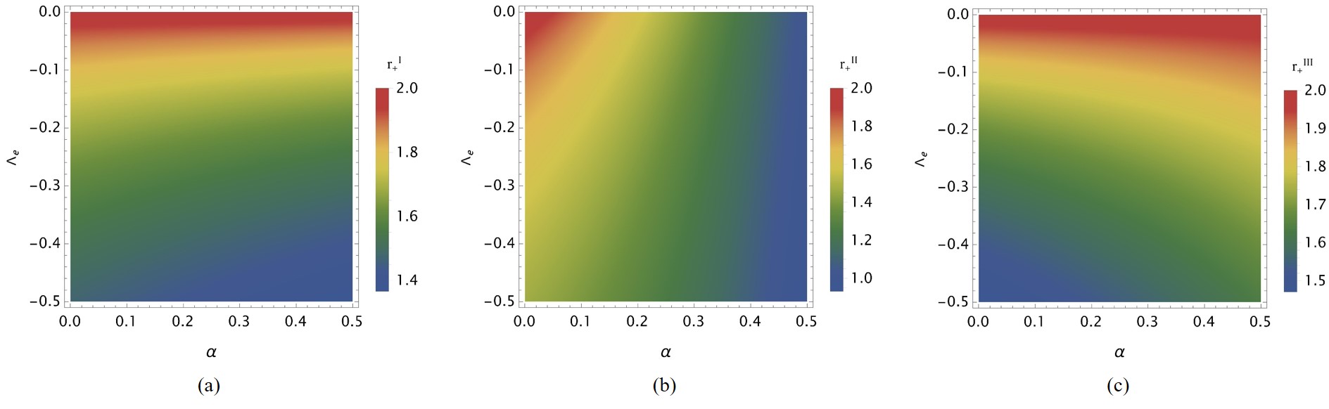
Figure 1: Horizon structure of black holes with LIV effects $\alpha$: (a) Case I, (b) Case II , and (c) Case III. We set $M^{\rm I}=M^{\rm II}=M^{\rm III}=1$.

In LIV gravity, neutral AdS black holes can exhibit modified horizon structures, as LIV not only redefines the effective cosmological constant but also introduces additional contributions to the horizon radius. However, these contributions do not change the number of horizons; rather, they result in a rescaling of the existing horizon radius. As we will see, this rescaling manifests as an inflation or constriction of the geometry, depending on the nature and magnitude of the LIV contributions. In this section, we quantify the horizon structure modifications for the three primary cases considered in this paper and discuss their implications within the framework of LIV physics.

Throughout, we use natural units with $c=G=\hbar=1$. A general static, spherically symmetric metric for an uncharged, non-rotating black hole in the context of LIV gravity can be expressed as Maluf and Neves (2021); Yang et al. (2023a); Liu et al. (2024)

$$\mathrm{d}s^{2}=g_{\rm tt}\mathrm{d}t^{2}+g_{\rm rr}\mathrm{d}r^{2}+r^{2}(\mathrm{d}\theta^{2}+\sin^{2}\theta\mathrm{d}\phi^{2}),$$ (17)

Here, $g_{\rm tt}$ and $g_{\rm rr}$ vary for each of the aforementioned cases described by the metrics in Eqs. (14), (15), and (16), as summarized in Table 1. To determine the event horizon radius, we set $g_{\rm tt}=0$ for each case. For Case I, we have

$$r_{+}^{\rm I}=-\frac{\mathcal{F}(M^{\rm I},\Lambda_{e},\alpha)^{1/3}}{(1+\alpha)\Lambda_{e}}-\frac{1}{\mathcal{F}(M^{\rm I},\Lambda_{e},\alpha)^{1/3}},$$ (18)

where

$$\mathcal{F}(M^{\rm I},\Lambda_{e},\alpha):= \sqrt{(1+\alpha)^{3}\Lambda_{e}^{3}\left[9(1+\alpha)\Lambda_{e}(M^{\rm I})^{2}-1\right]}$$ (19)

$$+3(1+\alpha)^{2}\Lambda_{e}^{2}M^{\rm I}.$$

For Case II, we get

$$r_{+}^{\rm II}=\frac{\mathcal{G}(M^{\rm II},\Lambda_{e},\alpha)^{1/3}}{(\alpha-1)\Lambda_{e}}+\frac{1}{\mathcal{G}(M^{\rm II},\Lambda_{e},\alpha)^{1/3}},$$ (20)

where

$$\mathcal{G}(M^{\rm II},\Lambda_{e},\alpha):= \sqrt{(\alpha-1)^{3}\Lambda_{e}^{3}\left[9(\alpha-1)^{3}\Lambda_{e}(M^{\rm II})^{2}+1\right]}$$ (21)

$$+3(\alpha-1)^{3}\Lambda_{e}^{2}M^{\rm II}.$$

Finally, for Case III, we have

$$r_{+}^{\rm III}=\frac{\mathcal{H}(M^{\rm III},\Lambda_{e},\alpha)^{2/3}+(1-\alpha)\Lambda_{e}}{(\alpha-1)\Lambda_{e}\mathcal{H}(M^{\rm III},\Lambda_{e},\alpha)^{1/3}},$$ (22)

where

$$\mathcal{H}(M^{\rm III},\Lambda_{e},\alpha):= \sqrt{(\alpha-1)^{3}\Lambda_{e}^{3}\left[9(\alpha-1)\Lambda_{e}(M^{\rm III})^{2}+1\right]}$$ (23)

$$+3(\alpha-1)^{2}\Lambda_{e}^{2}M^{\rm III}.$$

To understand the impact of LIV on neutral AdS black holes, we present density plots with $\Lambda_{e}$ and the LIV parameter $\alpha$, as shown in Fig. 1. Fig. 1 (a) corresponds to Case I, while Cases II and III are depicted in Fig. 1 (b) and (c), respectively. It is evident that for Case I and Case II, $\alpha$ reduces the size of the black hole, whereas it inflates the black hole size in Case III. Thus, for Case I and Case II, $\alpha$ serves a role analogous to that of electric charge in Reissner-Nordström geometry, while in Case III, it resembles the effects of dark energy Bhattacharya (2018); Bukhari et al. (2023). In this context, the LIV effects in Case III exhibit a quintessential character. In all three cases, however, the effective cosmological constant $\Lambda_{e}$ plays a similar role to the original cosmological constant, resulting in a reduction of the black hole size. At first glance, these observations of diminishing and inflating geometries of the black holes may appear trivial. However, as we will demonstrate in the following analyses of various thermodynamic potentials, these changes lead to nontrivial and anomalous characteristics in the spacetime endowed with LIV effects. It is important to note that we only consider positive values of $\alpha$ in our work, although negative values are also permissible Yang et al. (2023a).
Note that in a generic AdS spacetime the cosmological constant $\Lambda$ defines a characteristic AdS radius $L$, given by $L=\sqrt{-3/\Lambda}$. When LIV effects are introduced, an effective cosmological constant $\Lambda_{e}$ is defined, leading to a new AdS radius $L_{e}=\sqrt{-3/\Lambda_{e}}$. Consequently, the associated curvature of the AdS geometry, as defined by the Kretschmann scalar, is altered. Typically, a higher magnitude $|\Lambda_{e}|$ (corresponding to a smaller $L_{e}$) in an AdS black hole increases the spacetime curvature, and its impact is more pronounced in the asymptotic regions of spacetime. This can be understood as follows: consider, for example, the Kretschmann scalar $K$ for the Bumblebee black hole, as given by Maluf and Neves (2021)

$$K= \ R_{\mu\nu\gamma\delta}R^{\mu\nu\gamma\delta}$$

$$= \frac{8\Lambda_{e}^{2}}{3}+\frac{\alpha}{(1+\alpha)r^{2}}\Bigg{[}\frac{8\Lambda_{e}}{3}+\frac{4\alpha}{(1+\alpha)r^{2}}$$ (24)

$$+\frac{16M^{2}}{(1+\alpha)r^{3}}+\frac{48M^{2}}{\alpha(1+\alpha)^{2}r^{4}}\Bigg{]}.$$ (25)

where $R_{\mu\nu\gamma\delta}$ is the Riemann tensor. It is evident that the curvature is most pronounced in the vicinity of the black hole, where the majority of the contributions arise from the black hole mass $M$. In the asymptotic limit $r\rightarrow\infty$, the Kretschmann scalar approaches $K\approx\frac{8\Lambda_{e}^{2}}{3}$, indicating that the dominant contributions to the spacetime curvature originate from $\Lambda_{e}$. (Similar arguments apply to KR gravity models Yang et al. (2023a); Liu et al. (2024)). In addition to this, examining the asymptotic nature of spacetime requires considering the $r\rightarrow\infty$ limit for all three metrics (Cases I-III). For Case I, the metric components

$$g_{\rm tt}|_{r\rightarrow\infty}\approx\frac{(1+\alpha)\Lambda_{e}r^{2}}{3},\quad g_{\rm rr}^{-1}|_{r\rightarrow\infty}\approx-\frac{\Lambda_{e}r^{2}}{3},$$ (26)

indicate that the spacetime retains its AdS character at large distances, as the effective cosmological constant $\Lambda_{e}$ governs the asymptotic behavior. This property is similarly found in the other two KR gravity models, as thoroughly emphasized in Yang et al. (2023a); Liu et al. (2024).

III LIV-induced modification of thermodynamic properties of AdS black holes

As noted above, LIV-induced shifts in the horizon structure of AdS black holes directly influence their thermodynamic properties, such as temperature and entropy, both of which are sensitive to changes in horizon size. For example, $\alpha$ may increase the black hole temperature and alter the Hawking radiation spectrum. In this section, we provide a detailed analysis of these modifications across our chosen three cases of interest.

III.1 First law of black hole thermodynamics and LIV effects

By setting $-g_{\rm tt}=0$, we can obtain the mass $M$ of the black holes expressed in terms of $r_{+}$ for the three cases considered above (Cases I-III). Specifically, we have:

$$M^{\rm I} =\frac{1}{6}r_{+}^{\rm I}\left[3-(1+\alpha)\Lambda_{e}(r_{+}^{\rm I})^{2}\right],$$ (27)

$$M^{\rm II} =\frac{\left[3-(1-\alpha)\Lambda_{e}(r_{+}^{\rm II})^{2}\right]r_{+}^{\rm II}}{6(1-\alpha)},$$ (28)

$$M^{\rm III} =\frac{1}{6}r_{+}^{\rm III}\left[3-(1-\alpha)\Lambda_{e}(r_{+}^{\rm III})^{2}\right].$$ (29)

The quantity $M$ represents a measure of the internal energy of the black holes. From the first law of black hole mechanics,

$$\mathrm{d}M=T\mathrm{d}S+V\mathrm{d}P,$$ (30)

where $T$, $V$ and $P$ are the temperature, volume and pressure, respectively. The entropy of the black hole is given by the formula

$$S=\int\left(\frac{\partial M}{\partial T}\right)_{P}=\int\frac{1}{T}\left(\frac{\partial M}{\partial r_{+}}\right)_{P}\mathrm{d}r_{+}=\pi r_{+}^{2}.$$ (31)

This quantity is illustrated in Fig. 2 as a function of $M$, providing an effective description of the LIV AdS black hole system under fixed values of $\alpha$ and $\Lambda_{e}$. Specifically, the entropy plots for Case I are displayed in the first row, those for Case II in the second row, and Case III in the third row. As expected from the Bekenstein-Hawking entropy-area relation for black holes, the entropy increases with $M$. The influence of $\alpha$ is to reduce the entropy for a given value of $M$ in Cases I and II, which is consistent with $\alpha$ decreasing the size of the black hole horizon. Conversely, for Case III, where the LIV effects exhibit a quintessential character, the entropy increases.

It is noteworthy that as $\alpha$ varies, the entropy plots for all three cases shown in Fig. 2 become distinguishable for larger black hole sizes, while they converge at the origin. Assuming that LIV effects manifest around the quantum gravity scale, as is commonly proposed Liberati (2013), this suggests that the entropy curves for the three cases should diverge for black holes within the quantum regime, specifically near the Planck scale, corresponding to the region close to $r_{+}=0$. As the black hole size increases, the geometry transitions to a classical regime, rendering any LIV effects negligible. However, LIV effects present a different scenario. This discrepancy may stem from the additional fields coupled to the background geometry, which exert their influence even in the absence of a black hole or $\Lambda_{e}$ (i.e., when $M=\Lambda_{e}=0$), as demonstrated by the $g_{\rm rr}$ components of the three metrics (14), (15), and (16). In other words, LIV fields are intrinsically embedded within the spacetime geometry. Since LIV effects can imply a violation of rotational or translational invariance in spacetime, leading to an anisotropic energy-momentum tensor Liu et al. (2024), it is generally unreasonable to expect the entropy curves for different $\alpha$ values to converge for larger geometries.

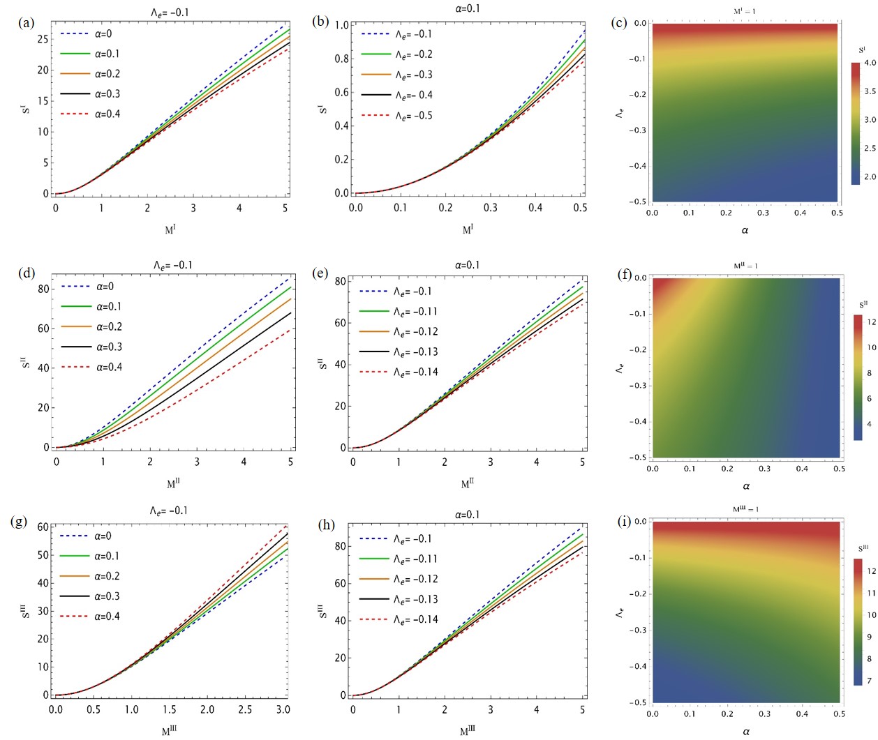
Figure 2: Entropy of the black holes vs mass $M$ for various $\alpha$ and $\Lambda_{e}$: from top, Case I (first row), Case II (second row), Case III (third row).

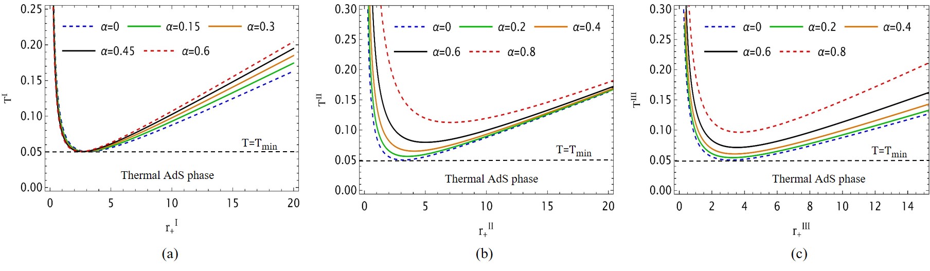
Figure 3: Hawking temperature $T$ vs. $r_{+}$ for various $\alpha$: (a) Case I, (b) Case II, and (c) Case III. We set $\Lambda_{e}=-0.1$.

III.2 Black hole temperature effects

By identifying a timelike Killing vector $\eta^{\mu}=\left(\frac{\partial}{\partial t}\right)^{\mu}$ and the surface gravity $\kappa=\sqrt{(\nabla^{\mu}\eta^{\nu})(\nabla_{\mu}\eta_{\nu})}$, the Hawking temperature can be computed as

$$T =\frac{\kappa}{2\pi}=-\frac{1}{4\pi\sqrt{-g_{\rm tt}g_{\rm rr}}}\frac{\partial g_{\rm tt}}{\partial r}\bigg{|}_{r=r_{+}}.$$ (32)

Thus, for the three cases considered here, we have:

$$T^{\rm I} =\frac{1-(\alpha+1)\Lambda_{e}(r_{+}^{\rm I})^{2}}{4\pi\sqrt{\alpha+1}r_{+}^{\rm I}},$$

$$T^{\rm II} =\frac{(\alpha-1)\Lambda_{e}(r_{+}^{\rm II})^{2}+1}{4\pi(1-\alpha)r_{+}^{\rm II}},$$

$$T^{\rm III} =\frac{(\alpha-3)\Lambda_{e}(r_{+}^{\rm III})^{2}+3}{12\pi\sqrt{1-\alpha}r_{+}^{\rm III}},$$ (33)

respectively. It is worth noting that the temperature can also be defined from the first law (30) as $T=\left(\frac{\mathrm{d}M}{\mathrm{d}S}\right)_{r=r_{+}}$, which can be easily verified to produce the same expression as derived earlier.

We next plot $T$ against the black hole size $r_{+}$ in Fig. 3, which exhibits a rich behavior across the three cases with respect to $\alpha$. For all three cases, the temperature curves possess a global minimum, $T_{\mathrm{min}}$, which can be determined using

$$\frac{\mathrm{d}T}{\mathrm{d}r_{+}}\bigg{|}_{r_{+}=r_{\mathrm{min}}}=0.$$ (34)

corresponding to a specific $r_{+}$. This particular black hole radius $r_{\mathrm{min}}$ marks the transition between small black holes (SBH) and large black holes (LBH), characterized by $r_{+}<r_{\mathrm{min}}$ and $r_{+}>r_{\mathrm{min}}$, respectively. Below $T_{\rm min}$, the system consists solely of thermal radiation, as indicated for all three cases. LBHs are generally stable, whereas SBHs are unstable, as will be evident from the free energy and heat capacity analyses of the black holes. We also note the presence of a pure radiation or AdS thermal phase below $T_{\mathrm{min}}$, as indicated for all three curves. In the pure radiation or thermal AdS phase, the background thermal bath is too cold to permit the nucleation of black hole phases Hawking and Page (1983). With the introduction of $\alpha$, we observe a continuous increase in temperature for the same black hole size across the three cases on larger geometric scales. The value of $r_{\mathrm{min}}$ is shifted due to $\alpha$, which, for the three cases, can be expressed as follows:

$$r^{\rm I}_{\mathrm{min}}=\frac{1}{\sqrt{(\alpha+1)|\Lambda_{e}|}},r^{\rm II}_{\mathrm{min}}=\frac{1}{\sqrt{(\alpha-1)\Lambda_{e}}},r^{\rm III}_{\mathrm{min}}=\sqrt{\frac{3}{(\alpha-3)\Lambda_{e}}},$$

giving rise to three different minimum temperatures:

$$T^{\rm I}_{\mathrm{min}} =\frac{\sqrt{|\Lambda_{e}|}}{2\pi}$$ (35)

$$T^{\rm II}_{\mathrm{min}} =-\frac{\Lambda_{e}}{2\pi\sqrt{(\alpha-1)\Lambda_{e}}}$$ (36)

$$T^{\rm III}_{\mathrm{min}} =\frac{\sqrt{(\alpha-3)\Lambda_{e}}}{2\pi\sqrt{3(1-\alpha)}},$$ (37)

for the three cases, respectively. For Case I, we note that $T^{\rm I}_{\mathrm{min}}$ is independent of $\alpha$, while the other two cases are not. This highlights a notable feature of the Bumblebee field model that distinguishes it from the corresponding KR field models. Additionally, for Case I, $r_{\rm min}^{\rm I}$ shifts toward lower values with each variation of $\alpha$, although the impact is minimal for the range of $\alpha$ considered here. In contrast, for the other two cases, the shift is toward larger values. These observations can also be inferred from the expressions in (35), (36), and (37). Next, we aim to elucidate the possible physical grounds underlying the behavior of the Hawking temperature.
If one associates the Hawking temperature of the black hole with a characteristic frequency, this temperature enhancement may crudely suggest an increase in the emission frequency of the black hole due to LIV backgrounds. Specifically, the enhancement of the Hawking temperature in all three cases, linked to increased emission frequency, can be interpreted analogously to blackbody emission, where the peak of the radiation shifts toward higher frequencies as the temperature rises. This analogy holds true, as black hole emission is fundamentally akin to blackbody radiation. One might consider this additional energy contribution (higher emission frequency) to arise from the energy density associated with the LIV fields. Alternatively, the modified dispersion relation for massless fields, characterized by energy $E$ and momentum $p$, associated with LIV effects is given by $E^{2}=p^{2}+\beta f(p)=0$ Gubitosi and Magueijo (2019), where $f(p)$ is a function dependent on the energy scale of the theory (with $\beta\rightarrow 0$ recovering the low-energy limit). This relation redefines the energy propagation speeds in spacetime and may therefore influence the frequency of the Hawking radiation perceived by a distant observer. The particle energy $E$ is further enhanced due to LIV fields, resulting in higher frequencies or energies being observed at asymptotic distances, which leads to enhanced temperature measurements for different values of $\alpha$. Therefore, with LIV-induced effects, black holes exhibit characteristic changes in their Hawking spectrum, which could serve as a significant signpost for quantum gravity considerations. This is particularly relevant as Hawking emission plays a foundational role in all quantum gravity theories Birrell and Davies (1982).
It is also noteworthy that the $\alpha$-independence of $T_{\rm min}^{\rm I}$, as shown in Eq. (35), may suggest that the LIV-field coupling to the spacetime geometry is activated only after the temperature increases and the black hole grows in size (LBH regime). In contrast, for KR fields, the coupling is established at very low temperatures, potentially just slightly above zero [see Fig. 3]. This perspective holds true if one envisions the formation of black holes in AdS spaces as a result of gravitational collapse within the AdS phase filled with thermal radiation, as described in Hawking and Page (1983). It is important to note that, under this framework, the temperature corresponds to the generalized temperature of the system, which may coincide with the Hawking temperature for values greater than or equal to $T_{\rm min}$ in all three cases.

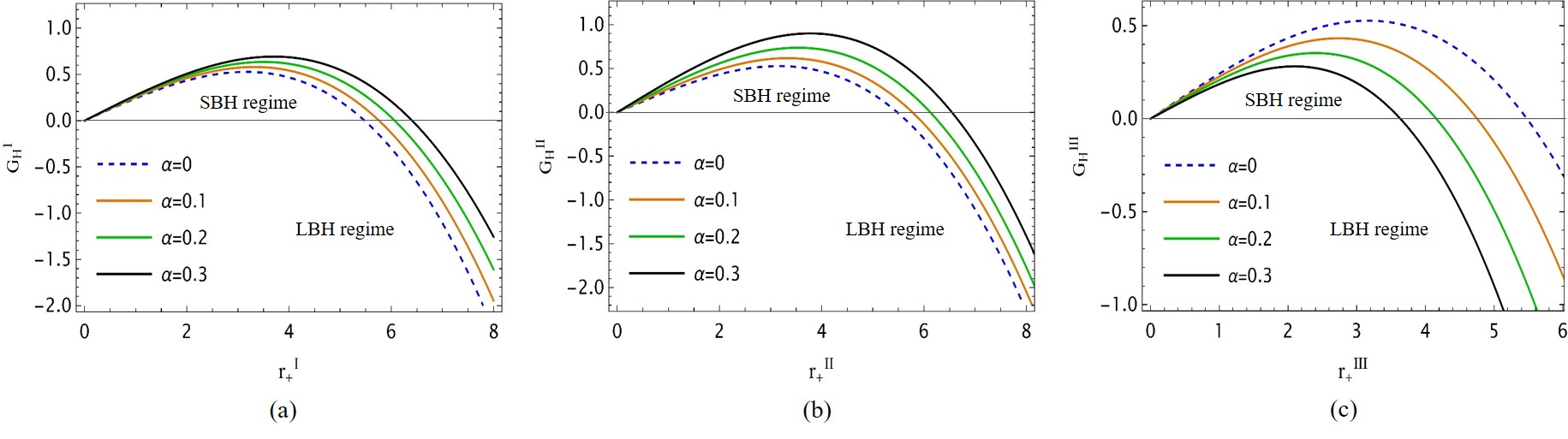
Figure 4: Free energy vs. $r_{+}$ for various $\alpha$: (a) Case I , (b) Case II, and (c) Case III. We chose $\Lambda_{e}=1$.

III.3 Gibbs free energy, black hole stability, pressure, and volume

Investigating the global stability of black holes is generally insightful and can be determined through the Gibbs free energy, given by $G_{\mathrm{H}}=M-TS$. In our case, this yields

$$G^{\rm I}_{\mathrm{H}} =-\frac{r_{+}^{\rm I}\left[1-(\alpha+1)\Lambda_{e}(r_{+}^{\rm I})^{2}\right]}{4\sqrt{\alpha+1}}-\frac{1}{6}r_{+}^{I}\left[(\alpha+1)\Lambda_{e}(r_{+}^{\rm I})^{2}-3\right],$$

$$G^{\rm II}_{\mathrm{H}} =\frac{r_{+}^{\rm II}\left[(\alpha-1)\Lambda_{e}(r_{+}^{\rm II})^{2}+3\right]}{6(1-\alpha)}-\frac{(r_{+}^{\rm II})^{2}\left[(\alpha-1)\Lambda_{e}(r_{+}^{\rm II})^{2}+1\right]}{4(1-\alpha)r_{+}},$$

$$G^{\rm III}_{\mathrm{H}} =\frac{1}{6}r_{+}^{\rm III}\left[(\alpha-1)\Lambda_{e}(r_{+}^{\rm III})^{2}+3\right]-\frac{r_{+}^{\rm III}\left[(\alpha-3)\Lambda_{e}(r_{+}^{\rm III})^{2}+3\right]}{12\sqrt{1-\alpha}},$$ (38)

and has been plotted in Fig. 4. Recalling that a positive (negative) $G_{\mathrm{H}}$ indicates an unstable (stable) black hole, the plots reveal two distinct regimes: a positive $G_{\mathrm{H}}$ regime corresponding to small black hole (SBH) scales and a negative $G_{\mathrm{H}}$ regime for large black hole (LBH) scales. Consequently, black holes are stable at larger scales and vice versa—a characteristic feature of asymptotically AdS black holes. Introducing $\alpha$ broadens the negative $G_{\mathrm{H}}$ regime, thereby favoring unstable SBHs. This effect holds for Case I and Case II only. In contrast, for Case III, the SBH regime is constrained, resulting in a thermodynamically more stable black hole phase while Hawking evaporation persists. Notably, this LBH/SBH transition constitutes a second-order thermodynamic phase transition, commonly observed in black holes beyond the simplest Schwarzschild geometry Davies (1978). Further discussion of this transition within the context of free energy landscape theory is presented in Sec. V.
Here, in general spacetime dimensions $d$, pressure $P$ is defined as Kubiznak et al. (2017)

$$P:=-\frac{\Lambda}{8\pi}=\frac{(d-1)(d-2)}{16\pi l^{2}}.$$ (39)

However, in the context of LIV gravity for $d=4$, as considered here, it must be redefined as

$$P:=-\frac{\Lambda_{e}}{8\pi},$$ (40)

which gives

$$P^{\rm I}=-\frac{\Lambda}{8(1+\alpha)\pi},P^{\rm II}=-\frac{\Lambda}{8(1-\alpha)\pi},P^{\rm III}=-\frac{\Lambda}{8(1-\alpha)\pi},$$ (41)

hence incorporating LIV effects through $\alpha$. Taking this relation for $P$ into account, we can deduce the following from Eq. (33):

$$P^{\rm I} =\frac{T^{\rm I}}{2\sqrt{1+\alpha}r_{+}^{\rm I}}-\frac{1}{8\pi(1+\alpha)(r_{+}^{\rm I})^{2}},$$ (42)

$$P^{\rm II} =\frac{T^{\rm II}}{2r_{+}^{\rm II}}-\frac{1}{8\pi(1-\alpha)(r_{+}^{\rm III})^{2}},$$ (43)

$$P^{\rm III} =\frac{3(\sqrt{1-\alpha})T^{\rm III}}{2(3-\alpha)r_{+}^{\rm III}}+\frac{3}{8\pi(\alpha-3)(r_{+}^{\rm III})^{2}}.$$ (44)

which represent the equations of state for the three cases and will be further explored in Sec. VI.

In LIV gravity models, such as those involving Bumblebee and KR fields, the redefinition of black hole thermodynamic quantities introduces unique implications for the black hole volume. Since the mass $M$ of the black hole in this formalism is interpreted as the gravitational analogue of enthalpy, rather than internal energy, we obtain a new perspective on how volume is treated within the black hole’s thermodynamic framework. This enthalpic viewpoint enables the definition of a thermodynamic volume, given by

$$V=\left(\frac{\partial M}{\partial P}\right)_{S}=\left(\frac{\partial M}{\partial\Lambda_{e}}\right)_{S}\left(\frac{\partial\Lambda_{e}}{\partial P}\right)_{S}\sim\frac{4}{3}\pi r_{+}^{3}.$$ (45)

Note that here the thermodynamic volume is not only related to the horizon radius but also to the field-driven modifications in pressure ($P$) and $\Lambda_{e}$, reflecting how LIV fields reshape the geometry around the black hole [see (18), (20), (22)]. In LIV gravity, the Bumblebee and KR fields alter the gravitational landscape around the black hole, influencing $\Lambda_{e}$ and its partial derivatives with respect to $M$ and $P$. This modification implies that the black hole’s enthalpy no longer depends solely on the cosmological constant in a straightforward manner but also on the contributions from the LIV fields. Consequently, the modified $\Lambda_{e}$ adjusts the thermodynamic volume, as the LIV fields effectively alter the “spatial stretching” or “compression” of the black hole horizon.

III.4 Heat capacity analysis

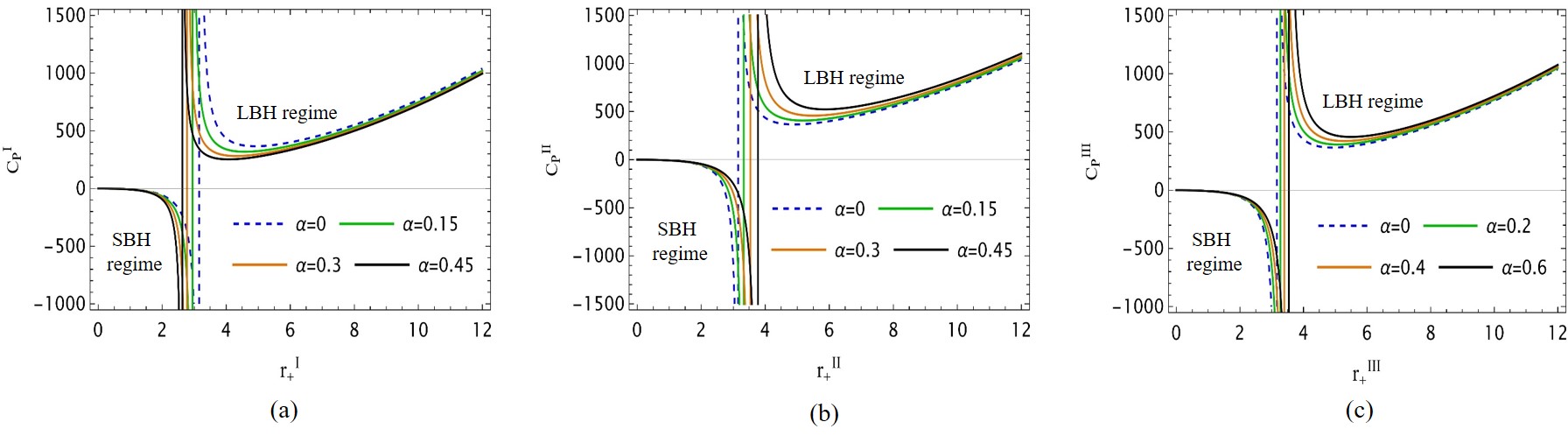
Figure 5: Heat capacity of the black holes with various choices of $\alpha$: from top, Case I (left), Case II (middle), Case III (right). The vertical lines depicts the point $r_{\mathrm{min}}$ for all the cases. Note that by fixing $\Lambda_{e}$, one has to treat above plots as effective description. We chose $\Lambda_{e}=1$.

Black holes in AdS space exhibit a range of notable thermodynamic processes that are absent in asymptotically flat spacetime. One prominent example is the Hawking-Page phase transition Hawking and Page (1983). In the presence of LIV fields, many geometric properties undergo modifications, as discussed earlier. Consequently, it is reasonable to expect that the associated heat capacity, which characterizes the different phases of the system and its critical points, is also altered in an LIV background. To quantify these effects, we begin by considering the standard definition of heat capacity at constant pressure

$$C_{\rm P}=T\left(\frac{\partial S}{\partial T}\right)_{P}=T\left(\frac{\partial S}{\partial r_{+}}\right)_{P}\left(\frac{\partial r_{+}}{\partial T}\right)_{P}.$$ (46)

For our three cases, this yields

$$C^{\rm I}_{\rm P} =\frac{2\pi(r_{+}^{\rm I})^{2}\left[(\alpha+1)\Lambda_{e}(r_{+}^{\rm I})^{2}-1\right]}{(\alpha+1)\Lambda_{e}(r_{+}^{\rm I})^{2}+1},$$ (47)

$$C^{\rm II}_{\rm P} =\frac{2\pi(r_{+}^{\rm II})^{2}\left[(\alpha-1)\Lambda_{e}(r_{+}^{\rm II})^{2}+1\right]}{(\alpha-1)\Lambda_{e}(r_{+}^{\rm II})^{2}-1},$$ (48)

$$C^{\rm III}_{\rm P} =\frac{2\pi(r_{+}^{\rm III})^{2}\left[(\alpha-3)\Lambda_{e}(r_{+}^{\rm III})^{2}+3\right]}{(\alpha-3)\Lambda_{e}(r_{+}^{\rm III})^{2}-3}.$$ (49)

These quantities are depicted in Fig. 5. The heat capacity expressions in Eqs. (47), (48), and (49) require careful examination.

Following our original definition of $\Lambda_{e}$, namely, $\Lambda_{e}=\Lambda/(1+\alpha)$ for Bumblebee gravity (Case I) and $\Lambda_{e}=\Lambda/(1-\alpha)$ for symmetric KR gravity (Case II), it is straightforward to observe that for the cases presented in Eqs. (47) and (48), $C_{\rm P}$ becomes fundamentally independent of $\alpha$. (This observation for Case II has already been noted in Ref. Yang et al. (2023a).) We propose that the impact of $\alpha$ can still be effectively analyzed by fixing $\Lambda_{e}$. It is well established that a positive (negative) value of $C_{\rm P}$ indicates local thermodynamic stability (instability) of the black hole Davies (1978). Examination of the plots reveals two distinct thermodynamic phases: a stable LBH phase and an unstable SBH phase, separated by an infinite discontinuity corresponding to $r_{\mathrm{min}}$ discussed earlier. For Case I, the discontinuity shifts towards lower $r_{+}^{I}$ values, whereas for the other cases, it shifts towards larger $r_{+}$ values. Additionally, $\alpha$ narrows the $C_{\rm P}$ parameter space for SBH in Case I, while it expands the parameter space for the other two cases. Consequently, if the growth of black holes in AdS space is envisioned as a nucleation process where radiation collapses gravitationally, it is reasonable to infer that the presence of the LIV field in the Bumblebee case accelerates the transition from SBH (unstable) to LBH (stable) compared to standard AdS black holes ($\alpha=0$). In contrast, for KR fields, the presence of LIV effects delays these transitions.
The unstable configuration of the SBH is a well-known feature of AdS black holes, attributed to the following reason Dolan (2011b): the negative cosmological constant induces a negative energy density. As the black hole radiates at constant $P$, the volume decreases, leading to an increase in vacuum energy (less negative). Simultaneously, the temperature rises, further increasing the vacuum energy. For stability, which requires $C_{\rm P}>0$, the cosmological constant must be sufficiently large. In the first two cases, this requirement is fulfilled by the original $\Lambda$. However, in the third case, the effective cosmological constant $\Lambda_{e}$ must fulfill this role, implying that Lorentz violation must be extremely small, thereby imposing stringent bounds on $\alpha$. This constraint is also evident from the temperature expressions provided in Eq. (33).

IV Hawking-Page phase transition

In standard AdS black hole thermodynamics, the Hawking-Page transition marks a critical temperature where there’s a phase transition between thermal radiation and a stable black hole configuration in AdS space. In the context of LIV gravity, this phase transition can reveal deviations in black hole thermodynamics due to altered symmetries, potentially influencing the stability conditions and critical points of the transition Hawking and Page (1983). By incorporating modifications to spacetime symmetries, LIV alters the metric structure and energy-momentum relations, which, for AdS black holes in LIV gravity, could result in distinctive thermodynamic properties, including shifts in the Hawking temperature, entropy, and specific heat capacities. Consequently, these changes may modify or even eliminate the conditions for the Hawking-Page transition, potentially giving rise to new phases or critical behaviors.

When considering black holes within a thermodynamic ensemble, two stable phases emerge: the thermal AdS phase and the large Schwarzschild-AdS black hole phase. In the thermal AdS phase, black holes are absent, and the system consists purely of radiation. At a critical temperature, $T_{\mathrm{HP}}$, these two phases are separated, marking a transition. This transition is classified as a first-order phase transition and, through the AdS/CFT correspondence Maldacena (1998), closely parallels the confinement/deconfinement transition observed in quantum chromodynamics (QCD) Witten (1998). The formation of black holes within thermal AdS spaces is particularly significant, as it impacts density fluctuations that potentially influenced structure formation in the early Universe Li and Wang (2020).

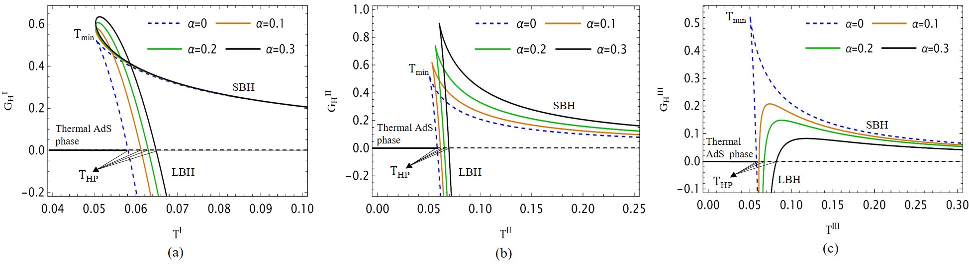
Figure 6: $G_{\mathrm{H}}$-$T$ plots indicating Hawking-Page transition for (a) Case I, (b) Case II, and (c) Case III, respectively. We chose $\Lambda_{e}=1$.

The comparison of Gibbs free energy $G$ versus temperature $T$ in AdS black holes allows for the identification of stable phases and the precise characterization of the Hawking-Page phase transition. Below the critical temperature $T_{\mathrm{HP}}$, the thermal AdS phase has a lower Gibbs free energy, indicating it as the thermodynamically preferred state. Above $T_{\mathrm{HP}}$, the large Schwarzschild-AdS black hole phase becomes energetically favorable, marking a first-order phase transition analogous to the liquid-gas transition in classical thermodynamics, where the intersection of Gibbs free energies signifies a shift between distinct thermodynamic phases.

Before addressing the LIV cases, we first outline the behavior of the Schwarzschild-AdS black hole, represented by dashed blue lines ($\alpha=0$) across all three plots. The graphical plots reveal three primary phases: SBH, LBH, and radiation. For the SBH phase, the free energy increases (becoming more positive) as temperature $T$ decreases, reaching a peak before descending. Along this segment, the black hole horizon radius $r_{+}$ increases along the curve (refer to Fig. 3 also). The point at which $G_{\rm H}=0$ marks the coexistence of the LBH and thermal AdS phases. In the thermal AdS or radiation phase, the free energy vanishes, given that the particle number associated with this radiation is negligible, as demonstrated by Hawking and Page Hawking and Page (1983). The peak corresponds to the minimum temperature, given in Eqs. (35), (36), and (37), as previously discussed and depicted in Fig. 3. From the perspective of heat capacity (Fig. 5), this is where the heat capacity exhibits an infinite discontinuity. Taken together, these features naturally indicate the stability of the LBH phase and the instability of the SBH phase.
The LBH branch, characterized by a positive heat capacity, also displays positive free energy. In contrast, the AdS space possesses zero free energy, establishing it as the globally preferred thermodynamic state, while the LBH remains locally stable within this regime. However, when the LBH acquires negative free energy, it transitions to become the globally preferred thermodynamic state. Notably, the classification into SBH/LBH is determined by the black hole radius, with $r_{+}<r_{\rm min}$ for SBH and $r_{+}>r_{\rm min}$ for LBH, where this distinction ultimately depends on the AdS radius, parameterized by $\Lambda_{e}$.
The transition from the LBH phase to the thermal AdS phase, referred to as the Hawking-Page transition, occurs at a critical temperature $T_{\rm HP}$ (the Hawking-Page temperature). At this temperature, the free energy remains continuous, while its first derivative exhibits a discontinuity, thereby characterizing the transition as a first-order phase transition, analogous to solid-liquid or liquid-gas phase transitions.

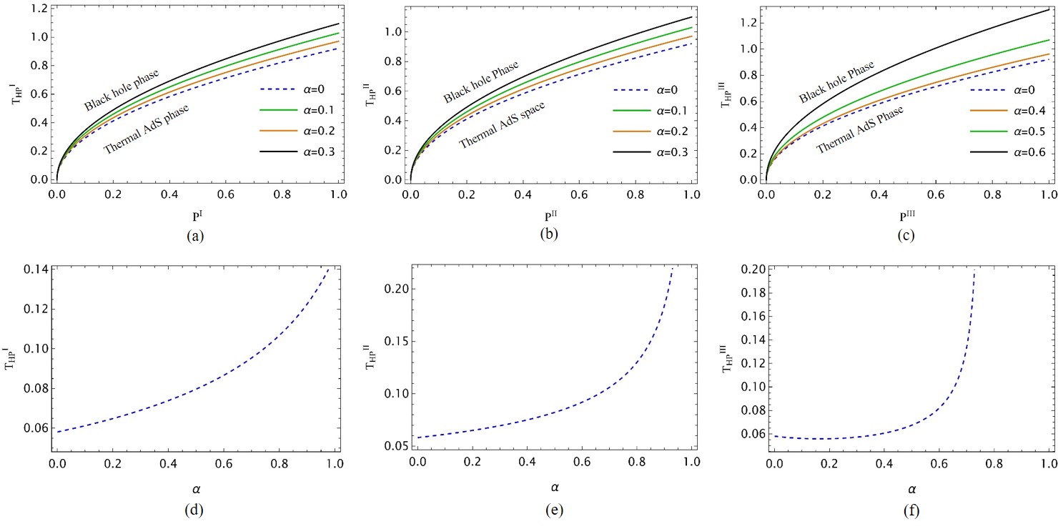
Figure 7: Hawking-Page critical temperature $T_{\mathrm{HP}}$ vs. pressure $P$ (first row), vs. $\alpha$ (second row) for Case I, Case II, and Case III, from left to right. Here, we set $\Lambda_{e}=-0.1$

IV.1 Case I: Bumblebee Model

When LIV effects are introduced ($\alpha\neq 0$), the phase transitions undergo notable modifications, as depicted in Fig. 6. In Case I, illustrated in Fig. 6(a), increasing $\alpha$ causes the peak of the free energy curves to shift and smoothens the previously sharp cusp. Furthermore, the Hawking-Page temperature $T_{\rm HP}^{\rm I}$ rises with each increment in $\alpha$. To elucidate this increase in $T_{\rm HP}^{\rm I}$, we calculate the Hawking-Page temperature by setting $G_{H}^{\rm{I}}=0$ in Eq. (38), which gives the critical radius $r_{+}:=r_{\rm{HP}}^{\rm I}$ as follows:

$$r_{\rm HP}^{\rm I}=\frac{\sqrt{3}\sqrt{2-\frac{1}{\sqrt{\alpha+1}}}}{\sqrt{\left(2\alpha-3\sqrt{\alpha+1}+2\right)\Lambda_{e}}}.$$ (50)

Substituting this expression into Eq. (33), we obtain the Hawking-Page temperature:

$$T_{\rm HP}^{\rm I}=\frac{-\sqrt{\alpha+1}\Lambda_{e}}{\sqrt{3}\pi\sqrt{2-\frac{1}{\sqrt{\alpha+1}}}\sqrt{\left(2\alpha-3\sqrt{\alpha+1}+2\right)\Lambda_{e}}}.$$ (51)

The above equation can also be expressed in terms of pressure as:

$$T_{\rm HP}^{\rm I}=\frac{\sqrt{\alpha+1}}{\sqrt{2-\frac{1}{\sqrt{\alpha+1}}}\sqrt{\left(3\sqrt{\alpha+1}-2\alpha-2\right)}}\sqrt{\frac{8P^{\rm I}}{3\pi}}.$$ (52)

This represents a coexistence line equation, which is depicted in Fig. 7(a). For the range of $\alpha$ considered here, the equation holds across all values of $\alpha$. To illustrate this relationship further, we plot $T_{\rm HP}^{\rm I}$ versus $P^{\rm I}$, representing the coexistence curves for the black hole and thermal AdS phases. For each fixed value of $P^{\rm I}$, the corresponding values of $T_{\rm HP}^{\rm I}$ increase with $\alpha$. These curves extend without bound across all possible values of $T_{\rm HP}^{\rm I}$ and $P^{\rm I}$. In the limit of vanishing LIV effects, $\alpha\rightarrow 0$, we recover

$$T_{\mathrm{HP}}=\sqrt{\frac{8P}{3\pi}},$$ (53)

which is the well-known result for Schwarzschild-AdS black holes Su et al. (2020).

The Hawking-Page transition temperature $T_{\rm HP}^{\rm I}$, marking the phase shift between thermal AdS space and the LBH state, increases in the presence of LIV effects parameterized by $\alpha$. This suggests that achieving a thermodynamically stable black hole state (characterized by negative Gibbs free energy $G_{\rm H}^{\rm I}$) via gravitational collapse of thermal radiation requires a higher energy input into the system. This observation extends to the behavior depicted in the coexistence curves [Fig. 7 (a)]. Furthermore, the ratio

$$\frac{T_{\rm HP}^{\rm I}}{T_{\rm min}^{\rm I}}=\frac{\sqrt{\alpha+1}}{\sqrt{2-\frac{1}{\sqrt{\alpha+1}}}\sqrt{3\sqrt{\alpha+1}-2\alpha-2}},$$ (54)

is just a number for a particular value of $\alpha$, and is independent of the pressure $P^{\rm I}$. This holds for any Bumblebee black hole within a specific range for $\alpha$, similarly to the Schwarzschild-AdS case Wei et al. (2020). This result confirms that the novel duality relation—where the Hawking-Page transition temperature corresponds to a dual minimum temperature of the black hole in an additional spatial dimension—holds in Bumblebee gravity.

IV.2 Case II: Symmetric KR Model

For Case II, the $G^{\rm II}_{\rm H}-T^{\rm II}$ plots in Fig. 6(b) indicate that the cusp marking the SBH/LBH transition remains intact, signifying an abrupt transition analogous to that observed in the Schwarzschild-AdS black hole. As in Case I, $T_{\rm HP}^{\rm II}$ increases with each increment in $\alpha$, accompanied by a corresponding rise in the free energy $G^{\rm II}_{\rm H}$. Under LIV effects, the slope of the LBH curves approaches infinity, suggesting that the system rapidly stabilizes in the globally thermodynamic stable LBH phase. The continuous increase in the free energy peak suggests an additional positive energy contribution to the system, likely from the LIV field energy density. Furthermore, the slower decline in free energy for the SBH phase at higher $T^{\rm II}$ indicates an increased thermodynamic instability in the SBH phase. Consequently, although the Hawking-Page transition from the thermal AdS phase to the LBH phase occurs at a higher $T^{\rm II}_{\rm HP}$, requiring greater energy input, the system nonetheless favors the LBH phase. Thus, in the presence of the KR field, the formation of a black hole state is energetically preferred.
To mathematically analyze the formation of the LBH phase, the critical radius is given by

$$r_{\rm HP}^{\rm II}=\frac{\sqrt{3}}{\sqrt{(\alpha-1)\Lambda_{e}}},$$ (55)

at which the Hawking-Page phase transition temperature is

$$T_{\rm HP}^{\rm II}=-\frac{\Lambda_{e}}{\sqrt{3}\pi\sqrt{(\alpha-1)\Lambda_{e}}}=\frac{1}{\sqrt{1-\alpha}}\sqrt{\frac{8P^{\rm II}}{3\pi}},$$ (56)

demonstrating that $T_{\rm HP}^{\rm II}$ is modified by an $\alpha$-dependent factor, similar to Case I. Clearly, from Eq. (56), any increase in $\alpha$ raises $T_{\rm HP}^{\rm II}$. Additionally, the duality relation between $T^{\rm II}_{\rm HP}$ and $T^{\rm II}_{\rm min}$, as defined in Eq. (54), remains constant and independent of $P^{\rm II}$, consistent with Wei et al. (2020). Thus, the KR field, like the Bumblebee field, preserves this bulk-boundary correspondence in the black hole-AdS system.

IV.3 Case III: Asymmetric KR Model

In this case, we observe a consistent decrease in free energy with increasing LIV effects, as illustrated in the $G_{\rm H}^{\rm III}-T^{\rm III}$ plots in Fig. 6(c). This behavior contrasts with the symmetric KR model observed in Case II. Here, the cusp at the LBH/SBH phase transition becomes smoother, indicating a gradual transition, potentially through metastable transient black hole states. Such a phase transition is reminiscent of the supercooled liquid phase of water as its temperature falls below the freezing point Wei and Liu (2020). Based on the energy interpretation provided in Cases I and II, one might not anticipate a free energy decrease due to the KR field. However, it is evident that the geometric contributions of the KR field in this case diverge from those in Case II (see Table 1). Consequently, assuming any direct thermodynamic resemblance to other cases would be an a priori assumption. Thus, the antisymmetric tensorial nature of the KR field sets it apart from both its symmetric counterpart in Case II and the Bumblebee model in Case I.
The critical radius at which Hawking-Page transition occurs is found to be

$$r_{\rm HP}^{\rm III}=\frac{\sqrt{3}}{\sqrt{(\alpha-1)\Lambda_{e}}}.$$ (57)

The corresponding Hawking-Page temperature reads

$$T_{\rm HP}^{\rm III} =-\frac{\Lambda_{e}}{\pi\sqrt{3\sqrt{1-\alpha}\left(2\sqrt{1-\alpha}-1\right)}\sqrt{\left[\left(\frac{1}{\sqrt{1-\alpha}}-2\right)\alpha-\frac{3}{\sqrt{1-\alpha}}+2\right]\Lambda_{e}}}$$

$$=\frac{1}{\sqrt{3\sqrt{1-\alpha}\left(2\sqrt{1-\alpha}-1\right)}\sqrt{\left[\frac{3}{\sqrt{1-\alpha}}-\left(\frac{1}{\sqrt{1-\alpha}}-2\right)\alpha-2\right]}}\sqrt{\frac{8P^{\rm III}}{3\pi}},$$ (58)

from which it is evident that $T^{\rm III}_{\rm HP}$ increases with $\alpha$. The ratio $T^{\rm III}_{\rm HP}/T^{\rm III}{\rm min}$ remains a constant independent of $P^{\rm III}$, supporting the conjecture proposed in Wei et al. (2020). Moreover, the $G^{\rm III}_{\rm H}-T^{\rm III}$ curves in Fig. 6(c) confirm that KR field effects predominantly influence the LBH regime. This finding is consistent with prior observations, indicating that LIV effects have a more pronounced impact on the global properties of the geometry, as reflected in other thermodynamic potentials such as entropy (Fig. 2) and free energy (Fig. 6).

V Generalized free energy landscape

The preceding discussion regarding thermodynamic phase behavior of black hole can be further realized with more insight using so-called free energy landscape Spallucci and Smailagic (2013); Li and Wang (2020). In this framework, one considers a canonical ensemble comprising a series of black hole thermodynamic states with a certain order parameter characterized by horizon radius of the black hole, ranging from zero to infinity. The order parameter for SBH and LBH is defined as simple horizon radii gotten by solving equations for Hawking temperature (33), assuming now the role of Hawking temperature being replaced by ensemble temperature $T$. The variation of ensemble temperature from lower to higher values encompasses all temperature considerations, including $T_{\rm min},T_{\rm HP}$, etc. Note that in this setting, the order parameter for thermal AdS phase which has no horizon radius is simply zero.

The Gibbs free energy is thus off-shell, defined as

$$G=M-TS=\frac{1}{6}r_{+}\left[3-(1+\alpha)\Lambda_{e}r_{+}^{2}\right]-\pi Tr_{+}^{2},$$ (59)

where $T$ is the generalized temperature of the ensemble of black holes. For each $T$, there is a $G-T$ plot which reflects different thermodynamic states for the system of black holes and thermal AdS space. We can analyze how the phase behavior of the system changes due to Lorentz violation, when $T$ changes from $T_{\mathrm{min}}$ onward. The three cases are discussed separately below.

V.1 Case I: Bumblebee Model

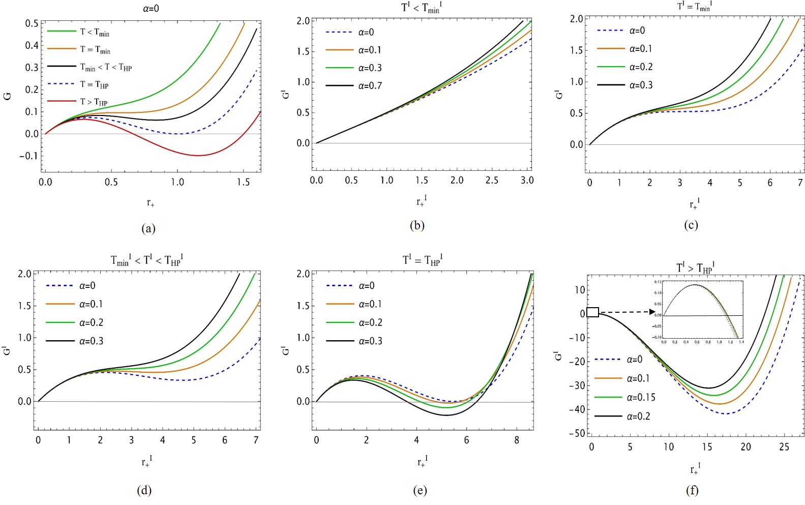
Figure 8: Generalized free energy landscape for Case I: Bumblebee model. We chose $\Lambda_{e}=-0.1$

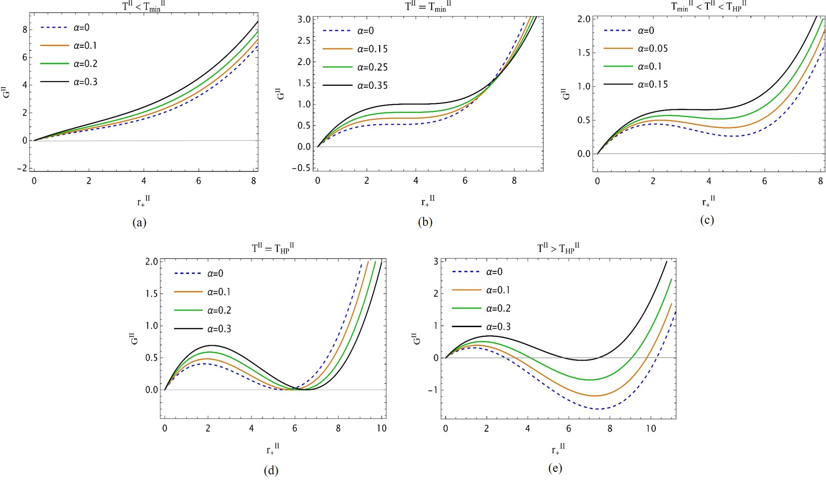
Figure 9: Generalized free energy landscape for Case II: symmetric KR model. We chose $\Lambda_{e}=-0.1$

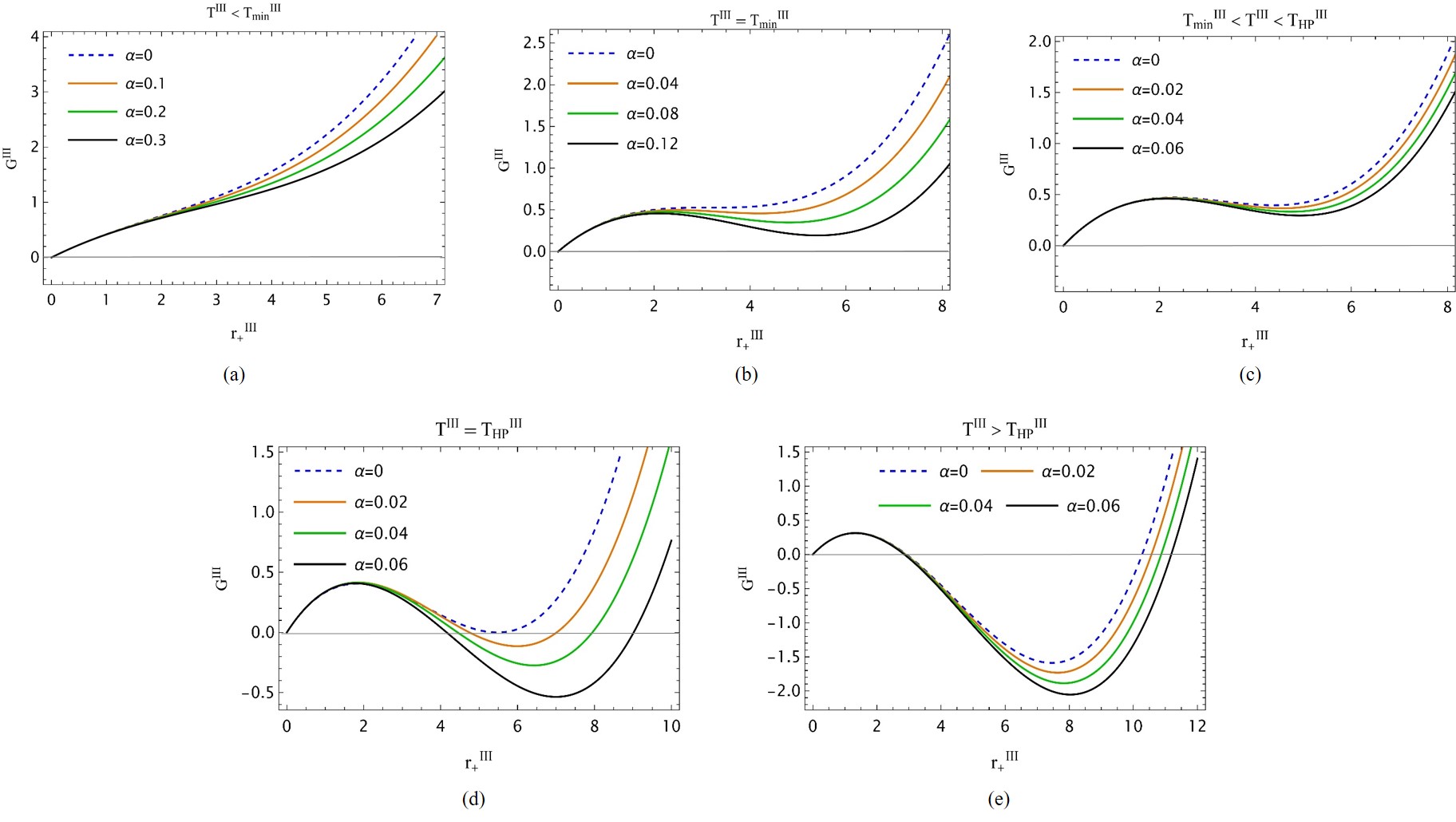
Figure 10: Generalized free energy landscape for Case III: asymmetric KR model. Here again, $\Lambda_{e}=-0.1$.

To understand the effect of LIV on the free energy landscape, it is essential to first examine the pure Schwarzschild-AdS system ($\alpha=0$), depicted in Fig. 8(a). For temperatures $T<T_{\rm min}$, the system has a single global minimum at $r_{+}=0$, corresponding to pure thermal radiation or the thermal AdS phase (green curve). When the temperature increases to $T=T_{\rm min}$, the Gibbs free energy exhibits an inflection point at $r_{+}=r_{\rm min}$, and the system consists of a single black hole (orange curve). For temperatures in the range $T_{\rm min}<T<T_{\rm HP}$ (black curve), two black hole solutions exist: a large black hole (LBH) and a small black hole (SBH), with radii given by Spallucci and Smailagic (2013):

$$r_{\rm l,s}=\frac{T}{2\pi T_{\rm min}^{2}}\left(1\pm\sqrt{1-\frac{T_{\rm min}^{2}}{T^{2}}}\right),$$ (60)

where $\pm$ corresponds to the LBH and SBH cases, respectively. Here, the SBH represents a local maximum of the Gibbs free energy, while the LBH corresponds to a local minimum. In this regime, the globally stable state remains thermal AdS. As the temperature approaches $T_{\rm HP}$ (dashed blue curve), the Gibbs free energy of the LBH and thermal AdS phase become degenerate at $r=r_{\rm HP}$, indicating a coexistence phase of the LBH and thermal AdS space. For temperatures $T>T_{\rm HP}$ (red curve), the global minimum of the Gibbs free energy shifts to the negative LBH branch, establishing it as the globally preferred state.

Let us now examine the role of LIV fields. Recalling from Eq. (33) for Case I, the temperature is given by

$$T^{\rm I}=\frac{1-(\alpha+1)\Lambda_{e}(r_{+}^{\rm I})^{2}}{4\pi\sqrt{\alpha+1}r_{+}^{\rm I}}.$$ (61)

Rewriting it as

$$(\alpha+1)\Lambda_{e}(r_{+}^{\rm I})^{2}+4\pi T\sqrt{1+\alpha}r_{+}^{\rm I}-1=0,$$ (62)

it becomes apparent that this is a quadratic equation with two real roots, given by

$$r_{\rm s,l}^{\rm I}=\frac{-2\pi T^{\rm I}\pm\sqrt{4\pi^{2}(T^{\rm I})^{2}+\Lambda_{e}}}{\sqrt{1+\alpha}\Lambda_{e}}.$$ (63)

Here, $\pm$ corresponds to the radii of the SBH and LBH, respectively. To ensure positivity of $r_{\rm s,l}^{\rm I}$, we must have $2\pi T^{\rm I}>\sqrt{4\pi^{2}(T^{\rm I})^{2}+\Lambda_{e}}$ as long as $\Lambda_{e}<0$, a condition that holds for all values of $T$ in this case. Furthermore, by requiring the term under the square root in Eq. (63) to be non-negative, we recover the expression for $T_{\rm min}^{\rm I}$ given in Eq. (35), ensuring that the radii are well-defined.

Note that the minimum black hole temperature, corresponding to $r_{\rm min}^{\rm I}=\frac{1}{\sqrt{(\alpha+1)|\Lambda_{e}|}}$, as given by Eq. (35), is

$$T_{\rm min}^{\rm I}=\frac{\sqrt{-\Lambda_{e}}}{2\pi},$$ (64)

which allows us to recast Eq. (63) into the following form:

$$r_{\rm l,s}^{\rm I}=\frac{T}{2\pi\sqrt{1+\alpha}(T_{\rm min}^{\rm I})^{2}}\left[1\pm\sqrt{1-\left(\frac{T_{\rm min}^{\rm I}}{T^{\rm I}}\right)^{2}}\right].$$ (65)

Evidently, the radii of both the SBH and LBH are modified by LIV effects through the parameter $\alpha$. These LIV effects reduce both the LBH and SBH sizes. In the limit where $\alpha\to 0$, we recover the Schwarzschild-AdS case (Eq. 60). It is also clear that for $T^{\rm I}<T_{\rm min}^{\rm I}$, Eq. (65) does not admit any black hole solutions, and the system is thus in the pure radiation phase. Thus, we may write the generalized off-shell free energy as

$$G^{\rm I} =M^{\rm I}-T^{\rm I}S^{\rm I}$$

$$=\frac{1}{6}r_{+}^{\rm I}\left[3-(1+\alpha)\Lambda_{e}(r_{+}^{\rm I})^{2}\right]-\pi T(r_{+}^{\rm I})^{2}.$$ (66)

The case $T^{\rm I}<T_{\rm min}^{\rm I}$ is depicted in Fig. 8(b). For each value of $\alpha$, the curve shifts upwards, resulting in an increase in the system’s free energy. Despite this shift, the system remains in the pure radiation phase, as the global minimum of the curve continues to be located at the origin ($r_{+}^{\rm I}=0$).

As the temperature approaches $T^{\rm I}=T_{\rm min}^{\rm I}$ [Fig. 8(c)], the free energy curves shift upward, and the inflection point is lost, akin to the $\alpha=0$ case. Thus, for any non-zero value of $\alpha$, the system is driven into the pure radiation phase, with the global minimum remaining at the origin. In the temperature range $T_{\rm min}^{\rm I}<T^{\rm I}<T_{\rm HP}^{\rm I}$, the system is expected to exhibit two black hole solutions: an unstable SBH and a locally stable LBH, with the thermal AdS phase being the globally preferred state. However, as shown in Fig. 8(d), LIV effects increase the free energy, potentially driving the system into a state where $T^{\rm I}\leq T_{\rm min}^{\rm I}$. At the Hawking-Page temperature $T^{\rm I}=T_{\rm HP}^{\rm I}$, illustrated in Fig. 8(e), LIV effects disrupt the Hawking-Page phase transition. For any non-zero value of $\alpha$, the system is forced into a state with negative free energy. Therefore, the degeneracy between thermal AdS and LBH is only preserved when $\alpha=0$. This suggests that LIV effects drive the system towards the globally favored LBH phase. Finally, for all $T^{\rm I}>T_{\rm HP}^{\rm I}$, as depicted in Fig. 8(f), LIV effects serve to reduce the global preference for the LBH phase by increasing the positive free energy. Interestingly, it is observed that $\alpha$ has a distinct impact on the free energy at $T^{\rm I}=T_{\rm HP}^{\rm I}$, in contrast to its effect at other temperature ranges.
As evident from the above, the system loses its well-defined boundaries between different thermodynamic phases due to the contributions of the Bumblebee field. This arises because the system is no longer governed by Lorentz-symmetric gravity. Therefore, it is reasonable to conclude that any observation of Hawking-Page thermodynamic behavior requires stringent constraints on LIV effects.

V.2 Case II: Symmetric KR Model

Analogous to Case I, we first derive the radii of the SBH and LBH: From (33), we have expression for the temperature as

$$T^{\rm II}=\frac{(\alpha-1)\Lambda_{e}(r_{+}^{\rm II})^{2}+1}{4\pi(1-\alpha)r_{+}^{\rm II}}$$ (67)

Applying the same procedure as in Case I, we obtain the two radii as

$$r_{l,s}^{\rm II}=\frac{2\pi\sqrt{1-\alpha}T^{\rm II}\pm\sqrt{4\pi^{2}(1-\alpha)(T^{\rm II})^{2}+\Lambda_{e}}}{-\sqrt{1-\alpha}\Lambda_{e}}.$$ (68)

Here, the $\pm$ sign denotes the solutions corresponding to the large and small black holes, respectively. The minimum temperature of the black hole, given by

$$T_{\rm min}^{\rm II}=-\frac{\Lambda_{e}}{2\pi\sqrt{(\alpha-1)\Lambda_{e}}},$$ (69)

corresponds to $r_{\rm min}^{\rm II}=\frac{1}{\sqrt{(\alpha-1)\Lambda_{e}}}$, which allows us to rewrite Eq. (68) as follows:

$$r_{\rm l,s}^{\rm II}=\frac{T^{\rm II}}{2\pi\sqrt{1-\alpha}(T_{\rm min}^{\rm II})^{2}}\left[1\pm\sqrt{1-\left(\frac{T_{\rm min}^{\rm II}}{T^{\rm II}}\right)^{2}}\right].$$ (70)

Once again, no black hole solutions are allowed for $T^{\rm II}<T_{\rm min}^{\rm II}$. Moreover, the SBH/LBH radii expand due to LIV effects, similar to the Bumblebee model. The generalized off-shell free energy is now given by:

$$G^{\rm II}= M^{\rm II}-T^{\rm II}S^{\rm II}$$

$$= \frac{1}{6}r_{+}^{\rm II}\left[3-(1+\alpha)\Lambda_{e}(r_{+}^{\rm II})^{2}\right]-\pi T(r_{+}^{\rm II})^{2},$$ (71)

and is graphically presented in Fig. 9.
As in the previous case, we include the $\alpha=0$ curve in each plot to emphasize the impact of LIV effects. From the plots, we observe that the temperature ranges $T^{\rm II}<T_{\rm min}^{\rm II}$, $T_{\rm min}^{\rm II}<T^{\rm II}<T_{\rm HP}^{\rm II}$, and $T^{\rm II}>T_{\rm HP}^{\rm II}$, shown in Figs. 9(a)-(c) and (e), exhibit behavior similar to that of Case I, with the free energy increasing as $\alpha$ is raised. Unlike the Bumblebee model, the system does not enter the negative free energy region at $T^{\rm II}=T_{\rm HP}^{\rm II}$; instead, the transition occurs at much larger radii $r^{\rm II}_{+}$. Additionally, we observe an enhancement in the free energy within the SBH regime, increasing its instability, as indicated in Figs. 9(c)-(e). Thus, in this case, the system loses its clear thermodynamic phase boundaries due to the influence of the KR field.

V.3 Case III: Asymmetric KR Model

In this section, we explore the free energy landscape of black holes within the context of the asymmetric KR model, as outlined in Table 1. The temperature expression, derived from Eq. (33), is given by:

$$T^{\rm III}=\frac{(\alpha-3)\Lambda_{e}(r_{+}^{\rm III})^{2}+3}{12\pi\sqrt{1-\alpha}r_{+}^{\rm III}},$$ (72)

The two black hole solutions in this case are given by

$$r_{\rm l,s}^{\rm III}=\frac{6\pi\sqrt{1-\alpha}T^{\rm III}\pm\sqrt{36\pi^{2}(1-\alpha)(T^{\rm III})^{2}-3(\alpha-3)\Lambda_{e}}}{(\alpha-3)\Lambda_{e}},$$ (73)

where $\pm$ denotes large and small black holes, respectively. Here, the minimum temperature corresponding to $r_{\rm min}^{\rm III}=\sqrt{\frac{3}{(\alpha-3)\Lambda_{e}}}$ turns out to be

$$T_{\rm min}^{\rm III}=\frac{\sqrt{(\alpha-3)\Lambda_{e}}}{2\pi\sqrt{3(1-\alpha)}}.$$ (74)

We thus make use of (74) to rewrite Eq. (73) as

$$r_{\rm l,s}^{\rm III}=\frac{T^{\rm III}}{2\pi\sqrt{1-\alpha}(T_{\rm min}^{\rm III})^{2}}\left[1\pm\sqrt{1-\left(\frac{T_{\rm min}^{\rm III}}{T^{\rm III}}\right)^{2}}\right].$$ (75)

This expression again indicates the absence of black hole solutions for $T<T^{\rm III}_{\rm min}$, while offering insight into how LIV effects modify the sizes of the SBH and LBH. The generalized free energy is then given by:

$$G^{\rm III} =M^{\rm III}-T^{\rm III}S^{\rm III}$$

$$=\frac{1}{6}r_{+}^{\rm III}\left[3-(1+\alpha)\Lambda_{e}(r_{+}^{\rm III})^{2}\right]-\pi T^{\rm III}(r_{+}^{\rm III})^{2}$$ (76)

which has been plotted in Fig. 10. We observe a general trend of a decrease in free energy across all temperature ranges, in contrast to the previous two cases. For $T^{\rm III}<T_{\rm min}^{\rm III}$, the curve shifts to lower values, indicating a reduction in positive free energy, thereby weakening the role of the AdS phase as the globally preferred thermodynamic state in this temperature range. In the next two temperature ranges, $T^{\rm III}=T_{\rm min}^{\rm III}$ and $T_{\rm min}^{\rm III}<T^{\rm III}<T_{\rm HP}^{\rm III}$, the decrease in free energy shows that LIV effects consistently push the system towards greater stability by disfavoring the SBH phase. At $T^{\rm III}=T_{\rm HP}^{\rm III}$ [Fig. 10(d)], the system acquires sufficient negative free energy, allowing it to settle into the LBH phase as the globally preferred thermodynamic state. This is similar to the situation observed in Case I for the Bumblebee model. Similarly, for $T^{\rm III}>T_{\rm HP}^{\rm III}$, as shown in Fig. 10(e), the LIV effects exhibit the same characteristics.

One is inevitably confronted with the question of the physical mechanism underlying the seemingly “disordered” behavior observed, especially in contrast to the pure Schwarzschild-AdS black hole. In this regard, we make the following observations. In standard AdS black holes, the geometry is asymptotically AdS, where the negative cosmological constant can be interpreted as a form of negative energy embedded in the spacetime Dolan (2011b). While the inclusion of Bumblebee Kostelecky (2004); Maluf and Neves (2021) or KR Yang et al. (2023a); Liu et al. (2024) fields does not alter the asymptotic AdS-like structure of spacetime, as discussed in Sec. II, the additional vector or tensorial field couplings to the gravitational background lead to deviations from the standard Hawking-Page paradigm. This deviation is likely a result of the interaction between the AdS spacetime and LIV fields, a relationship that, to the best of our knowledge, has not yet been rigorously established.

VI Microstructure of the black holes

Thermodynamic geometry provides a powerful framework for probing the thermal stability of systems exhibiting fluctuations around equilibrium configurations. Its origins can be traced back to the work of Weinhold Weinhold (1975a, b) and Ruppeiner Ruppeiner (1979, 1981, 2014), who proposed the possibility of defining a metric space involving the system’s extensive parameters, akin to Riemannian geometry. This formalism led to the definition of a Ricci scalar curvature, which reflects the underlying interactions among the system’s constituents, or microstates Ruppeiner (1995). These concepts have been applied not only to well-known fluctuating systems, such as magnetic systems, the Ising model, and quantum liquids Ruppeiner (1979, 1981); Janyszek and Mrugala (1989); Ruppeiner (2014), but also to more exotic systems, including black holes Ruppeiner (2014). Therefore, it is reasonable to expect that Ruppeiner geometry could offer valuable insights into how LIV influences microstate interactions, potentially uncovering distinct thermodynamic signatures or curvature structures that differ from those observed in relativistic cases.
We begin with the standard Boltzmann entropy relation, $S=k_{\rm B}\ln\Omega$, where $\Omega=\exp{\left(S/k_{\rm B}\right)}$ represents the number of microstates of the system. The two variables $x^{0}$ and $x^{1}$ characterize the black hole. As fluctuations occur in the system, the probability of transitioning to $x^{0}+\mathrm{d}x^{0}$ and $x^{1}+\mathrm{d}x^{1}$ is given by the expression $P(x^{0},x^{1})\,\mathrm{d}x^{0}\,\mathrm{d}x^{1}=\beta\Omega(x^{0},x^{1})\,\mathrm{d}x^{0}\,\mathrm{d}x^{1}$, with $\beta$ being a normalization constant. This leads to the relation $P(x^{0},x^{1})\propto\exp{\left(S/k_{\rm B}\right)}$, and we express the total entropy as

$$S(x^{0},x^{1})=S_{\rm BH}(x^{0},x^{1})+S_{\rm E}(x^{0},x^{1}),$$

where $S_{\rm BH}$ and $S_{\rm E}$ represent the black hole entropy and the entropy of the external environment, respectively. Suppose a small fluctuation occurs in the equilibrium entropy $S_{0}$ around the configuration $x_{0}^{\mu}$ (with $\mu,\nu=0,1$). Expanding in a Taylor series, we obtain:

$$S =S_{0}+\frac{\partial S_{\rm BH}}{\partial x^{\mu}}\bigg{|}_{x^{\mu}=x_{0}^{\mu}}\Delta x_{\rm bh}^{\mu}+\frac{\partial S_{\rm E}}{\partial x^{\mu}}\bigg{|}_{x^{\mu}=x_{0}^{\mu}}\Delta x_{\rm E}^{\mu}$$

$$+\frac{1}{2}\frac{\partial^{2}S_{\rm BH}}{\partial x^{\mu}\partial x^{\nu}}\bigg{|}_{x^{\mu}=x_{0}^{\mu}}\Delta x_{\rm bh}^{\mu}\Delta x_{\rm bh}^{\nu}+\frac{1}{2}\frac{\partial^{2}S_{\rm E}}{\partial x^{\mu}\partial x^{\nu}}\bigg{|}_{x^{\mu}=x_{0}^{\mu}}\Delta x_{\rm E}^{\mu}\Delta x_{\rm E}^{\nu}+\cdots,$$ (77)

We next assume that the system is closed such that $x_{\rm bh}^{\mu}+x_{\rm E}^{\mu}=x_{\rm total}^{\mu}=\text{constant}$, leading to

$$\frac{\partial S_{\rm BH}}{\partial x^{\mu}}\bigg{|}_{x^{\mu}=x_{0}^{\mu}}\Delta x_{\rm bh}^{\mu}=-\frac{\partial S_{\rm E}}{\partial x^{\mu}}\bigg{|}_{x^{\mu}=x_{0}^{\mu}}\Delta x_{\rm E}^{\mu}.$$ (78)

It is straightforward to demonstrate that

$$\Delta S =\frac{1}{2}\frac{\partial^{2}S_{\rm BH}}{\partial x^{\mu}\partial x^{\nu}}\bigg{|}_{x^{\mu}=x_{0}^{\mu}}\Delta x_{\rm bh}^{\mu}\Delta x_{\rm bh}^{\nu}+\frac{1}{2}\frac{\partial^{2}S_{\rm E}}{\partial x^{\mu}\partial x^{\nu}}\bigg{|}_{x^{\mu}=x_{0}^{\mu}}\Delta x_{\rm E}^{\mu}\Delta x_{\rm E}^{\nu}.$$ (79)

It is evident that $S_{\rm E}\sim S$, implying that the fluctuations in $S_{\rm E}$ are negligible, leaving only the black hole contribution. Therefore, we write (with $k_{\rm B}=1$)

$$P(x^{0},x^{1})\propto\exp{\left(-\frac{1}{2}\Delta l^{2}\right)},\ \Delta l^{2}=g_{\mu\nu}\Delta x^{\mu}\Delta x^{\nu},$$ (80)

with the metric $g_{\mu\nu}=-\frac{\partial^{2}S_{\rm BH}}{\partial x^{\mu}\partial x^{\nu}}$. It is important to note that $\Delta l^{2}$ measures the distance between two neighboring fluctuating states Ruppeiner (2014). Dropping the subscript $\rm BH$, we obtain

$$g_{\mu\nu}=-\frac{\partial^{2}S}{\partial x^{\mu}\partial x^{\nu}},$$ (81)

which represents the metric of the Ruppeiner geometry, allowing for the evaluation of the curvature scalar Carroll (2019)

$$\begin{aligned} R&=-\frac{1}{\sqrt{g}}\left[\frac{\partial}{\partial x^{0}}\left(\frac{g_{01}}{g_{00}\sqrt{g}}\frac{\partial g_{00}}{\partial x^{1}}-\frac{1}{\sqrt{g}}\frac{\partial g_{11}}{\partial x^{0}}\right)\right.\\[6.0pt] &\left.+\frac{\partial}{\partial x^{1}}\left(\frac{2}{\sqrt{g}}\frac{\partial g_{01}}{\partial x^{0}}-\frac{1}{\sqrt{g}}\frac{\partial g_{00}}{\partial x^{1}}-\frac{g_{01}}{g_{00}\sqrt{g}}\frac{\partial g_{00}}{\partial x^{0}}\right)\right],\end{aligned}$$ (82)

with $g:=\det{g_{\mu\nu}}=g_{00}g_{11}-g_{01}^{2}$. The curvature of the Ruppeiner metric in black hole systems is typically interpreted as a measure of the “interaction strength” between microstates. Positive curvature indicates repulsive interactions, which are associated with an unstable system, while negative curvature suggests attractive interactions, often linked to thermodynamically stable configurations. Divergences in the curvature scalar are often indicative of critical phenomena, such as phase transitions.

Based on the choice of extensive variables, the following length elements can be defined:

1. $\{P,V\}$-space: Here, both pressure and volume fluctuate:

   $$d\mathrm{l}^{2}=g_{PP}\mathrm{d}P^{2}+2g_{PV}\mathrm{d}P\mathrm{d}V+g_{VV}\mathrm{d}V^{2}.$$ (83)

2. $\{T,P\}$-space: Here, both temperature and pressure fluctuate:

   $$d\mathrm{l}^{2}=g_{\rm tt}\mathrm{d}T^{2}+2g_{TP}\mathrm{d}T\mathrm{d}P+g_{PP}\mathrm{d}P^{2}.$$ (84)

3. $\{T,V\}$-space: Here, both temperature and volume fluctuate:

   $$d\mathrm{l}^{2}=g_{\rm tt}\mathrm{d}T^{2}+2g_{TV}\mathrm{d}T\mathrm{d}V+g_{VV}\mathrm{d}V^{2}.$$ (85)

For all these metrics, the associated curvature can be easily defined using (82). (It is worth mentioning that various other formulations of thermodynamic geometry have been developed in recent years.)

Starting from the first law of thermodynamics $\mathrm{d}M=T\mathrm{d}S+V\mathrm{d}P$, we have

$$\mathrm{d}S=\frac{1}{T}\mathrm{d}M-\frac{V}{T}\mathrm{d}P.$$ (86)

Taking $(M,P)$ as the metric space, one obtains $\frac{\partial S}{\partial x^{\mu}}=\left(\frac{1}{T},\frac{-V}{T}\right)$, which, when applied to Eq. (80), leads to a universal form for the line element Xu et al. (2020):

$$\Delta l^{2}=\frac{1}{T}\Delta T\Delta S+\frac{1}{T}\Delta V\Delta P,$$ (87)

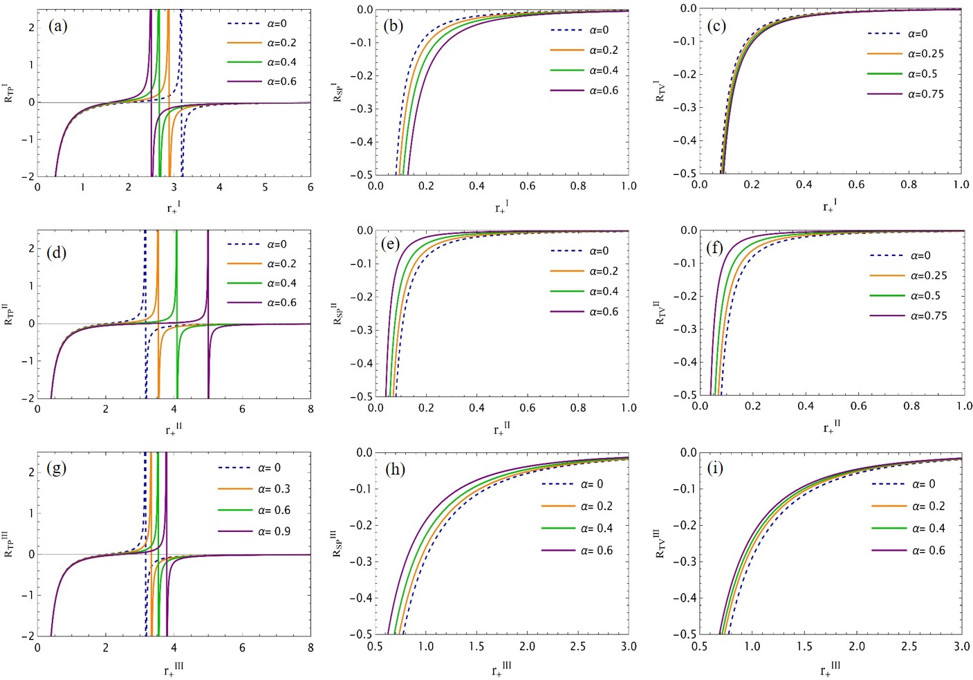
Figure 11: Thermodynamic curvatures of the black holes with various choices of $\alpha$: from top, first row : Case I (left), Case II (middle), Case III (right). $\Lambda_{e}=-0.1$ is chosen throughout.

It is evident that the line elements for four distinct metric spaces, $\{S,P\}$, $\{T,V\}$, $\{S,V\}$, and $\{T,P\}$, corresponding to various thermodynamic potentials, can be expressed as follows:

1. For the $\{S,P\}$-space, where enthalpy is the thermodynamic potential:

   $$\Delta l^{2} =\frac{1}{T}\left(\frac{\partial T}{\partial S}\right)_{P}\Delta S^{2}\quad+\frac{2}{T}\left(\frac{\partial T}{\partial P}\right)_{S}\Delta S\Delta P$$ (88)

   $$\quad+\frac{1}{T}\left(\frac{\partial V}{\partial P}\right)_{S}\Delta P^{2}.$$

2. For the $\{T,V\}$-space, where Helmholtz free energy is the thermodynamic potential:

   $$\Delta l^{2} =\frac{1}{T}\left(\frac{\partial S}{\partial T}\right)_{V}\Delta T^{2}\quad+\frac{2}{T}\left(\frac{\partial S}{\partial V}\right)_{T}\Delta T\Delta V$$ (89)

   $$\quad+\frac{1}{T}\left(\frac{\partial P}{\partial V}\right)_{T}\Delta V^{2}.$$

3. For the $\{S,V\}$-space, where Helmholtz free energy is the thermodynamic potential:

   $$\Delta l^{2}=\frac{1}{T}\left(\frac{\partial T}{\partial S}\right)_{V}\Delta S^{2}+\frac{1}{T}\left(\frac{\partial P}{\partial V}\right)_{S}\Delta V^{2}.$$ (90)

4. For the $\{T,P\}$-space, where Helmholtz free energy is the thermodynamic potential:

   $$\Delta l^{2}=\frac{1}{T}\left(\frac{\partial S}{\partial T}\right)_{P}\Delta T^{2}+\frac{1}{T}\left(\frac{\partial V}{\partial P}\right)_{T}\Delta P^{2}.$$ (91)

Since Legendre transformations exist between different thermodynamic potentials, all the above metrics are equivalent and thus represent the same underlying quantity Xu et al. (2021). Given that enthalpy $M$ and pressure $P$ are mutually linearly dependent, we can compute the second derivative $\frac{\partial^{2}M}{\partial P^{2}}$. Therefore, tor the $\{T,P\}$-space, the following curvature scalar can be formulated Miao and Xu (2018); Xu et al. (2021):

$$R_{\mathrm{TP}}=\frac{\partial}{\partial S}\left[\ln{\left(\frac{T}{\partial T/\partial P}\right)}\right],$$ (92)

where we utilize the definitions of $S$, $T$, and $P$ from Eqs. (31), (32), and (42), respectively, to express the curvature in terms of the horizon radius $r_{+}$. Similarly, for the $\{S,P\}$ and $\{T,V\}$ spaces, the corresponding curvature scalars are given by Xu et al. (2020):

$$R_{\mathrm{SP}}=\frac{-1}{S(1+8PS)},\ \ \ R_{\mathrm{TV}}=-\frac{1}{3\pi TV}.$$ (93)

Next, these thermodynamic formulations will be systematically applied to enhance our understanding of the physics of AdS black holes in a LIV gravity.

VI.1 Case I: Bumblebee Model

For the three major cases, using the expression for entropy, pressure and volume, the above curvature scalars turn out to be

$$R_{\rm TP}^{\rm I} =\frac{(\alpha+1)\Lambda_{e}(r_{+}^{\rm I})^{2}\left[2-(\alpha+1)\Lambda_{e}(r_{+}^{\rm I})^{2}\right]+1}{\pi(r_{+}^{\rm I})^{2}\left[(\alpha+1)^{2}\Lambda_{e}^{2}(r_{+}^{\rm I})^{4}-1\right]},$$ (94)

$$R_{\rm SP}^{\rm I} =\frac{2\sqrt{\alpha+1}}{\pi(r_{+}^{\rm I})^{2}\left[3\sqrt{\alpha+1}+5(\alpha+1)\Lambda_{e}(r_{+}^{\rm I})^{2}-5\right]},$$ (95)

$$R_{\rm TV}^{\rm I} =\frac{\sqrt{\alpha+1}}{\pi(r_{+}^{\rm I})^{2}\left[(\alpha+1)\Lambda_{e}(r_{+}^{\rm I})^{2}-1\right]}.$$ (96)

which bear LIV effects.

It is easier to analyze the LIV effects graphically. We plot the corresponding curvature scalars against the black hole size in Fig. 11. The first row corresponds to Case I. For the curvature scalar $R_{\rm TP}^{\rm I}$ [Fig. 11(a)], the plot indicates that the black hole remains in an ideal state for all larger sizes ($R_{\rm TP}^{\rm I}=0$). As Hawking evaporation occurs, the black hole size is reduced to shorter-distance scales, where the behavior of the system changes. We observe an infinite discontinuity in $R_{\rm TP}^{\rm I}$, which separates the negative regime from the positive one, similar to the behavior of the heat capacity $C_{\rm P}^{\rm I}$. This suggests that attractive interactions dominate the black hole at small scales before the phase transition occurs, at which point the black hole becomes unstable (positive curvature). The final negative divergence in the curvature indicates that the black hole undergoes a transition to a stable state. Since this divergence occurs at $C_{\rm P}^{\rm I}=0$, it may be linked to the black hole singularity at the origin ($r_{+}^{\rm I}=0$), and could potentially be a mathematical artifact. However, the first divergence occurs precisely at the point where the LBH and SBH coexist, i.e., $r_{+}^{\rm I}=1/\sqrt{(\alpha+1)\Lambda_{e}}$. This coincides exactly with the divergence in the heat capacity, as shown in Eq. (47).
The correspondence between the divergences and the zeros of the heat capacity with the curvature scalar suggests that thermodynamic geometry is a valuable tool for probing the black hole system in this context. Another noteworthy observation is the shifting of the divergence of $R_{\rm TP}^{\rm I}$ towards smaller black hole sizes as $\alpha$ increases. In this case, the ideal phase of the black hole persists longer due to the LIV effects. As for the other two curvature scalars, $R_{\rm SP}^{\rm I}$ and $R_{\rm TV}^{\rm I}$, shown in Figs. 11(b) and (c), the divergence occurs only at the origin, while the black hole remains in a stable phase throughout the evaporation process. As $\alpha$ causes the curvature scalars to become more negative, it can be inferred that LIV effects contribute to the stability of the black holes in this scenario.

VI.2 Case II: Symmetric KR model

Following the procedure outlined in the preceding section, the three curvature scalars are directly given by

$$R_{\rm TP}^{\rm II} =\frac{(\alpha-1)\Lambda_{e}(r_{+}^{\rm II})^{2}\left[(r_{+}^{\rm II})^{2}\Lambda_{e}(1-\alpha)-2\right]+1}{\pi(r_{+}^{\rm II})^{2}\left[(\alpha-1)^{2}\Lambda_{e}^{2}(r_{+}^{\rm II})^{4}-1\right]},$$ (97)

$$R_{\rm SP}^{\rm II} =\frac{\alpha-1}{(r_{+}^{\rm II})^{2}\left[\pi(\alpha-1)\Lambda_{e}(r_{+}^{\rm II})^{2}+\pi\right]},$$ (98)

$$R_{\rm TV}^{\rm II} =\frac{\alpha-1}{(r_{+}^{\rm II})^{2}\left[\pi(\alpha-1)\Lambda_{e}(r_{+}^{\rm II})^{2}+\pi\right]}.$$ (99)

These quantities are plotted in Figs. 11(d)-(f), where we observe that the infinite discontinuity shifts towards larger black hole sizes, indicating that phase transitions occur earlier with LIV effects. In contrast to the Bumblebee case, the curvature scalars $R_{\rm SP}^{\rm II}$ and $R_{\rm TV}^{\rm II}$ increase for a fixed $r_{+}^{\rm II}$, suggesting that the black hole becomes less stable as LIV effects are introduced. Divergences in the curvature still occur at $r_{+}^{\rm II}=\frac{1}{\sqrt{(\alpha-1)\Lambda_{e}}}$ for $R_{\rm TP}^{\rm II}$, corresponding to the behavior of the heat capacity [Eq. (48)]. Additionally, LIV effects do not alter the divergences in $R_{\rm SP}^{\rm II}$ and $R_{\rm TV}^{\rm II}$ at the origin.

VI.3 Case III: Asymmetric KR Model

Using Eqs. (92) and (93), the curvature scalars for this case are given by:

$$R_{\rm TP}^{\rm III} =\frac{(\alpha-3)\Lambda_{e}(r_{+}^{\rm III})^{2}\left[-\left\{(\alpha-3)\Lambda_{e}(r_{+}^{\rm III})^{2}\right\}-6\right]+9}{\pi(r_{+}^{\rm III})^{2}\left[(\alpha-3)^{2}\Lambda_{e}^{2}(r_{+}^{\rm III})^{4}-9\right]},$$ (100)

$$R_{\rm SP}^{\rm III} =-\frac{3\sqrt{1-\alpha}}{\pi(r_{+}^{\rm III})^{2}\left[(\alpha-3)\Lambda_{e}(r_{+}^{\rm III})^{2}+3\right]},$$ (101)

$$R_{\rm TV}^{\rm III} =-\frac{3\sqrt{1-\alpha}}{\pi(r_{+}^{\rm III})^{2}\left[(\alpha-3)\Lambda_{e}(r_{+}^{\rm III})^{2}+3\right]}.$$ (102)

The results are plotted in Fig. 11(g)-(i) for the three curvature scalars, respectively. In all three cases, we observe similarities to Case II. Additionally, a divergence for $R_{\rm TP}^{\rm III}$ is found at $r_{+}^{\rm III}=\frac{\sqrt{3}}{\sqrt{(\alpha-3)\Lambda_{e}}}$, which coincides with the divergence observed in the heat capacity. Thus, thermodynamic geometry provides an effective diagnostic tool for probing the underlying interactions among the black hole constituents.
From the above discussion, although the curves exhibit similar geometric behavior for the black holes, notable differences emerge, especially in their phase transition dynamics at short-distance scales. Specifically, the presence of Bumblebee or KR fields can either delay or accelerate phase transitions in evaporating black holes, depending on the type of curvature scalar. Regarding the ideal gas-like behavior of black holes at larger scales, which reflects a balance between attractive and repulsive interactions, it is important to consider that black holes may provide more space (or volume) to their constituents compared to the short-distance regime. In fact, it has been demonstrated that thermal fluctuations dominate black hole systems at smaller scales Faizal et al. (2017). Consequently, these fluctuations, which may signify a higher probability of intermolecular interactions, diminish as the black hole geometry increases in size, leading to an ideal gas-like phase. At smaller scales, the black hole geometry exhibits more chaotic behavior among its constituents, which amplifies the dominance of certain types of interactions, resulting in distinct (stable or unstable) phase behaviors, as inferred from the curvature scalar.
Furthermore, we have highlighted the equivalence of all thermodynamic metrics given in Eqs. (88)-(91), a fact that may not be immediately apparent from the plots in Fig. (82) for a particular case of the LIV model. To clarify this, we recall that thermodynamic geometry serves as an approximate framework designed to capture potential interactions among the constituents of a system. This approach holds even for simpler thermodynamic systems with which we are more familiar Ruppeiner (2014). The complexity is further compounded by the exotic nature of black hole systems. It is possible that the phase transitions indicated by divergences in the curvature scalar, after straightforward computation, could be a mathematical artifact Wei et al. (2019). This is analogous to the situation in black holes described in Schwarzschild coordinates, where the metric singularity at the event horizon arises solely due to a poor choice of coordinates and can be removed through an appropriate coordinate transformation Carroll (2019).

Figure 12: Energy emission rates of black holes in presence of LIV effects $\alpha$: (a) Case I, (b) Case II, and (c) Case III. Peak of the emission rate lowers for Bumblebee gravity, but increases for KR gravity. We chose $\Lambda_{e}=-0.1$ and $r_{+}=2$ throughout

VII Energy emission rates

As observed in the preceding discussion, LIV background fields modify the spacetime structure, thereby affecting the Hawking radiation spectrum. The modified Hawking emission not only unveils new regimes in the thermodynamics of AdS black holes but also alters the characteristic spectral distribution of LIV fields in the Hawking flux Hawking (1974, 1975). It is important to note that Hawking emission is a subtle phenomenon that occurs under specific conditions, influenced by the nature of the observer and the quantum vacuum states within black hole geometries Birrell and Davies (1982). The LIV-induced modifications to the emission power spectrum discussed here may suggest a potential directional dependence introduced into the background geometry by the presence of Bumblebee and KR fields.

Hawking evaporation is a process that occurs under the assumption of thermal equilibrium, where the black hole is in thermal balance with its surroundings. Although this assumption is idealized, it can be understood as follows: if the black hole’s temperature remains constant between successive emissions, the process can be effectively described using the canonical ensemble framework Kanti (2004). The energy emission rates can typically be determined using the well-established formula Hawking (1975)

$$\frac{\mathrm{d}^{2}E}{\mathrm{d}t\mathrm{d}\omega}=\frac{1}{2\pi}\sum_{\ell}\mathcal{N}_{\ell}\left|\mathcal{A}_{\ell}\right|^{2}\frac{\omega}{\exp{\left(\omega/T\right)}-1}.$$ (103)

Here, $\mathcal{N}_{\ell}$ represents the multiplicities, which depend on the spacetime dimensions, the number of particle species, and the angular momentum quantum number $\ell$. The terms $\mathcal{A}_{\ell}$ denote the greybody factors, $\omega$ is the frequency of the emitted radiation as measured by a distant observer, and $T$ is the Hawking temperature of the black hole, as defined in Eq. (33). For the case of electromagnetic fields, Eq. (103) simplifies to the following expression: Wei and Liu (2013); Papnoi et al. (2014)

$$E_{\omega t}:=\frac{\mathrm{d}^{2}E(\omega)}{\mathrm{d}\omega\mathrm{d}t}=\frac{2\pi^{2}\sigma\omega^{3}}{\exp{\left(\omega/T\right)}-1},$$ (104)

where $\sigma:=\pi r_{+}^{2}$ represents the cross-sectional area of the black hole, with $r_{+}$ being the horizon radius. For the three cases under consideration, we obtain:

$$E_{\omega t}^{\rm I} =\frac{2\pi^{3}(r_{+}^{\rm I})^{2}\omega^{3}}{\exp{\left[\frac{4\pi\sqrt{\alpha+1}r_{+}^{\rm I}\omega}{1-(\alpha+1)\Lambda_{e}(r_{+}^{\rm I})^{2}}\right]}-1},$$ (105)

$$E_{\omega t}^{\rm II} =\frac{2\pi^{3}(r_{+}^{\rm II})^{2}\omega^{3}}{\exp{\left[\frac{4\pi(1-\alpha)r_{+}^{\rm II}\omega}{(\alpha-1)\Lambda_{e}(r_{+}^{\rm II})^{2}+1}\right]}-1},$$ (106)

$$E_{\omega t}^{\rm III} =\frac{2\pi^{3}(r_{+}^{\rm III})^{2}\omega^{3}}{\exp{\left[\frac{12\pi\sqrt{(1-\alpha)}r_{+}^{\rm III}\omega}{(\alpha-3)\Lambda(r_{+}^{\rm III})^{2}+3}\right]}-1}.$$ (107)

Each case incorporates LIV effects through the parameter $\alpha$. To illustrate the impact of LIV, we present graphical representations in Fig. 12. Figures 12(a)-(c) show the emission rates for the three cases as a function of $\alpha$. Notably, the effect of $\alpha$ on Case I [Fig. 12(a)] differs from the other two cases, as the peak of the emission rate progressively decreases with increasing $\alpha$. In contrast, for the other two cases, an increase in $\alpha$ results in an enhancement of the energy emission. This behavior can be understood as follows. The emission rate reflects the speed at which the black hole evaporates. Since these black holes reside within AdS spacetime that incorporates an LIV background, the effects of LIV extend into the asymptotic regions. For a distant observer, the presence of the Bumblebee field would enhance the black hole’s evaporation, leading to a more rapid disappearance compared to a pure AdS background. In contrast, the KR field would suppress the evaporation rate, resulting in a slower rate of black hole evaporation. This distinction emphasizes that, despite the many similarities between Bumblebee and KR fields, they exhibit significant differences, with Hawking evaporation serving as a key example.

VIII Summary and outlooks

The phenomenology of LIV spacetime is of critical importance for the Standard Model Extension in particle physics and quantum gravity theories. One of the simplest models is Bumblebee gravity, where a vector field couples to the geometric background of spacetime. Similarly, KR gravity arises from an antisymmetric tensor field that couples to spacetime. In both models, a nonzero vacuum expectation value of the field generates new geometric structures, extending beyond standard Einstein gravity. Recently, significant progress has been made in deriving black hole solutions within these models. In the present work, we considered black hole solutions with a negative cosmological constant within both Bumblebee and KR gravity, and analyzed in detail the thermodynamic behavior of these black hole systems. Specifically, two frameworks were employed: the first based on the formalism of the free energy landscape, defined via a canonical ensemble approach, and the second on Ruppeiner thermodynamic geometry.
For the free energy landscape, we found that, under general conditions, the traditional Hawking-Page paradigm was disrupted by the range of LIV effects considered. Key parameters that characterized the phenomenon, such as the minimum temperature $T_{\rm min}$ and the Hawking-Page transition temperature $T_{\rm HP}$, were modified. Specifically, we observed that $T_{\rm HP}$ increased nonlinearly with LIV effects for all three cases, while this behavior was observed for $T_{\rm min}$ only in the case of KR fields. In different regimes of the free energy landscape, LIV effects caused one configuration to cross over into another regime.
We calculated the thermodynamic scalar curvature for the three cases using Ruppeiner geometry. Our analysis revealed that black holes at larger scales exhibited behavior akin to an ideal gas, whereas their behavior changed at short-distance scales. At these smaller scales, black holes underwent multiple stable and unstable phase transitions, characterized by infinite discontinuities. These transitions ultimately converged to the origin with a negatively divergent curvature. The infinite discontinuities were found to correspond to divergences in the heat capacity, which distinguished small black holes from their larger counterparts.
We also computed the particle emission rates and observed a suppression in the peak emission rates for Bumblebee gravity, while KR gravity showed an enhancement. This distinct power spectrum profile for the Bumblebee and KR fields indicates that, compared to Einstein gravity, black holes would evaporate more slowly in the case of Bumblebee gravity and more rapidly in the case of KR gravity.
Our study focused solely on neutral AdS black holes in LIV backgrounds, representing the simplest LIV extension of AdS black holes. However, a much richer range of phenomena has been observed for charged black holes, such as Reissner-Nordström and Kerr-Newman black holes. For example, charged AdS black holes exhibit van der Waals-like phase transitions, similar to those seen in ordinary liquids Kubiznak et al. (2017). Investigating such phenomena within LIV backgrounds could uncover intriguing physics and provide promising avenues for future research.

References

- Mariz et al. (2023) T. Mariz, J. R. Nascimento, and A. Petrov, Lorentz Symmetry Breaking—Classical and Quantum Aspects, SpringerBriefs in Physics (Springer, 2023) arXiv:2205.02594 [hep-th] .
- Tasson (2014) J. D. Tasson, Rept. Prog. Phys. 77, 062901 (2014), arXiv:1403.7785 [hep-ph] .
- Kostelecky and Samuel (1989a) V. A. Kostelecky and S. Samuel, Phys. Rev. D 39, 683 (1989a).
- Bluhm and Kostelecky (2005) R. Bluhm and V. A. Kostelecky, Phys. Rev. D 71, 065008 (2005), arXiv:hep-th/0412320 .
- Alfaro et al. (2002) J. Alfaro, H. A. Morales-Tecotl, and L. F. Urrutia, Phys. Rev. D 65, 103509 (2002), arXiv:hep-th/0108061 .
- Gambini and Pullin (1999) R. Gambini and J. Pullin, Phys. Rev. D 59, 124021 (1999), arXiv:gr-qc/9809038 .
- Carroll et al. (2001) S. M. Carroll, J. A. Harvey, V. A. Kostelecky, C. D. Lane, and T. Okamoto, Phys. Rev. Lett. 87, 141601 (2001), arXiv:hep-th/0105082 .
- Dubovsky et al. (2005) S. L. Dubovsky, P. G. Tinyakov, and I. I. Tkachev, Phys. Rev. Lett. 94, 181102 (2005), arXiv:hep-th/0411158 .
- Jacobson and Mattingly (2001) T. Jacobson and D. Mattingly, Phys. Rev. D 64, 024028 (2001), arXiv:gr-qc/0007031 .
- Horava (2009) P. Horava, Phys. Rev. D 79, 084008 (2009), arXiv:0901.3775 [hep-th] .
- Liberati (2013) S. Liberati, Class. Quant. Grav. 30, 133001 (2013), arXiv:1304.5795 [gr-qc] .
- Kostelecky (2004) V. A. Kostelecky, Phys. Rev. D 69, 105009 (2004), arXiv:hep-th/0312310 .
- Colladay and Kostelecky (2001) D. Colladay and V. A. Kostelecky, Phys. Lett. B 511, 209 (2001), arXiv:hep-ph/0104300 .
- Kostelecky and Lehnert (2001) V. A. Kostelecky and R. Lehnert, Phys. Rev. D 63, 065008 (2001), arXiv:hep-th/0012060 .
- Kostelecky and Lane (1999) V. A. Kostelecky and C. D. Lane, J. Math. Phys. 40, 6245 (1999), arXiv:hep-ph/9909542 .
- Yoder and Adkins (2012) T. J. Yoder and G. S. Adkins, Phys. Rev. D 86, 116005 (2012), arXiv:1211.3018 [hep-ph] .
- Colladay and McDonald (2009) D. Colladay and P. McDonald, Phys. Rev. D 79, 125019 (2009), arXiv:0904.1219 [hep-ph] .
- Mouchrek-Santos and Ferreira (2017) V. E. Mouchrek-Santos and M. M. Ferreira, Phys. Rev. D 95, 071701 (2017), [Erratum: Phys.Rev.D 100, 099901 (2019)], arXiv:1611.05336 [hep-ph] .
- Abazov et al. (2012) V. M. Abazov et al. (D0), Phys. Rev. Lett. 108, 261603 (2012), arXiv:1203.6106 [hep-ex] .
- Berger et al. (2016) M. S. Berger, V. A. Kostelecký, and Z. Liu, Phys. Rev. D 93, 036005 (2016), arXiv:1509.08929 [hep-ph] .
- Bailey (2009) Q. G. Bailey, Phys. Rev. D 80, 044004 (2009), arXiv:0904.0278 [gr-qc] .
- Tso and Bailey (2011) R. Tso and Q. G. Bailey, Phys. Rev. D 84, 085025 (2011), arXiv:1108.2071 [gr-qc] .
- Maluf et al. (2013) R. V. Maluf, V. Santos, W. T. Cruz, and C. A. S. Almeida, Phys. Rev. D 88, 025005 (2013), arXiv:1304.2090 [hep-th] .
- Bluhm et al. (2008a) R. Bluhm, S.-H. Fung, and V. A. Kostelecky, Phys. Rev. D 77, 065020 (2008a), arXiv:0712.4119 [hep-th] .
- Bailey and Kostelecky (2006) Q. G. Bailey and V. A. Kostelecky, Phys. Rev. D 74, 045001 (2006), arXiv:gr-qc/0603030 .
- Amelino-Camelia et al. (1998) G. Amelino-Camelia, J. R. Ellis, N. E. Mavromatos, D. V. Nanopoulos, and S. Sarkar, Nature 393, 763 (1998), arXiv:astro-ph/9712103 .
- Mattingly (2005) D. Mattingly, Living Rev. Rel. 8, 5 (2005), arXiv:gr-qc/0502097 .
- Addazi et al. (2022) A. Addazi et al., Prog. Part. Nucl. Phys. 125, 103948 (2022), arXiv:2111.05659 [hep-ph] .
- Piran and Ofengeim (2024) T. Piran and D. D. Ofengeim, Phys. Rev. D 109, L081501 (2024), arXiv:2308.03031 [astro-ph.HE] .
- Cao et al. (2024) Z. Cao et al. (LHAASO), Phys. Rev. Lett. 133, 071501 (2024), arXiv:2402.06009 [astro-ph.HE] .
- Kostelecky and Samuel (1989b) V. A. Kostelecky and S. Samuel, Phys. Rev. D 40, 1886 (1989b).
- Kostelecky and Samuel (1989c) V. A. Kostelecky and S. Samuel, Phys. Rev. Lett. 63, 224 (1989c).
- Bluhm et al. (2008b) R. Bluhm, N. L. Gagne, R. Potting, and A. Vrublevskis, Phys. Rev. D 77, 125007 (2008b), [Erratum: Phys.Rev.D 79, 029902 (2009)], arXiv:0802.4071 [hep-th] .
- Casana et al. (2018) R. Casana, A. Cavalcante, F. P. Poulis, and E. B. Santos, Phys. Rev. D 97, 104001 (2018), arXiv:1711.02273 [gr-qc] .
- Maluf and Neves (2021) R. V. Maluf and J. C. S. Neves, Phys. Rev. D 103, 044002 (2021), arXiv:2011.12841 [gr-qc] .
- Mai et al. (2023) Z.-F. Mai, R. Xu, D. Liang, and L. Shao, Phys. Rev. D 108, 024004 (2023), arXiv:2304.08030 [gr-qc] .
- An (2024) Y.-S. An, Phys. Dark Univ. 45, 101520 (2024), arXiv:2401.15430 [gr-qc] .
- Kanzi and Sakallı (2019) S. Kanzi and I. Sakallı, Nucl. Phys. B 946, 114703 (2019), arXiv:1905.00477 [hep-th] .
- Ovgün et al. (2018) A. Ovgün, K. Jusufi, and I. Sakalli, Annals Phys. 399, 193 (2018), arXiv:1805.09431 [gr-qc] .
- Yang et al. (2019) R.-J. Yang, H. Gao, Y. Zheng, and Q. Wu, Commun. Theor. Phys. 71, 568 (2019), arXiv:1809.00605 [gr-qc] .
- Cai and Yang (2023) Z. Cai and R.-J. Yang, Phys. Dark Univ. 42, 101292 (2023), arXiv:2205.04826 [gr-qc] .
- Oliveira et al. (2021) R. Oliveira, D. M. Dantas, and C. A. S. Almeida, EPL 135, 10003 (2021), arXiv:2105.07956 [gr-qc] .
- Zhang et al. (2023) X. Zhang, M. Wang, and J. Jing, Sci. China Phys. Mech. Astron. 66, 100411 (2023), arXiv:2307.10856 [gr-qc] .
- Amarilo et al. (2024) K. M. Amarilo, M. B. F. Filho, A. A. A. Filho, and J. A. A. S. Reis, Phys. Lett. B 855, 138785 (2024), arXiv:2307.10937 [gr-qc] .
- Xu et al. (2023) R. Xu, D. Liang, and L. Shao, Astrophys. J. 945, 148 (2023), arXiv:2302.05671 [gr-qc] .
- Kalb and Ramond (1974) M. Kalb and P. Ramond, Phys. Rev. D 9, 2273 (1974).
- Altschul et al. (2010) B. Altschul, Q. G. Bailey, and V. A. Kostelecky, Phys. Rev. D 81, 065028 (2010), arXiv:0912.4852 [gr-qc] .
- Kao et al. (1996) W. F. Kao, W. B. Dai, S.-Y. Wang, T.-K. Chyi, and S.-Y. Lin, Phys. Rev. D 53, 2244 (1996).
- Kar et al. (2003) S. Kar, S. SenGupta, and S. Sur, Phys. Rev. D 67, 044005 (2003), arXiv:hep-th/0210176 .
- Chakraborty and SenGupta (2017) S. Chakraborty and S. SenGupta, JCAP 07, 045 (2017), arXiv:1611.06936 [gr-qc] .
- Kumar et al. (2020) R. Kumar, S. G. Ghosh, and A. Wang, Phys. Rev. D 101, 104001 (2020), arXiv:2001.00460 [gr-qc] .
- Nair and Thomas (2022) K. K. Nair and A. M. Thomas, Phys. Rev. D 105, 103505 (2022), arXiv:2112.11945 [gr-qc] .
- Mukhopadhyaya et al. (2004) B. Mukhopadhyaya, S. Sen, S. Sen, and S. SenGupta, Phys. Rev. D 70, 066009 (2004), arXiv:hep-th/0403098 .
- Fu et al. (2012) C.-E. Fu, Y.-X. Liu, K. Yang, and S.-W. Wei, JHEP 10, 060 (2012), arXiv:1207.3152 [hep-th] .
- Lessa et al. (2020) L. A. Lessa, J. E. G. Silva, R. V. Maluf, and C. A. S. Almeida, Eur. Phys. J. C 80, 335 (2020), arXiv:1911.10296 [gr-qc] .
- Yang et al. (2023a) K. Yang, Y.-Z. Chen, Z.-Q. Duan, and J.-Y. Zhao, Phys. Rev. D 108, 124004 (2023a), arXiv:2308.06613 [gr-qc] .
- Liu et al. (2024) W. Liu, D. Wu, and J. Wang, JCAP 09, 017 (2024), arXiv:2406.13461 [hep-th] .
- Filho et al. (2024) A. A. A. Filho, J. A. A. S. Reis, and H. Hassanabadi, JCAP 05, 029 (2024), arXiv:2309.15778 [gr-qc] .
- Duan et al. (2024) Z.-Q. Duan, J.-Y. Zhao, and K. Yang, Eur. Phys. J. C 84, 798 (2024), arXiv:2310.13555 [gr-qc] .
- Du et al. (2024) Y.-Z. Du, H.-F. Li, Y.-B. Ma, and Q. Gu, (2024), arXiv:2403.20083 [hep-th] .
- Junior et al. (2024) E. L. B. Junior, J. T. S. S. Junior, F. S. N. Lobo, M. E. Rodrigues, D. Rubiera-Garcia, L. F. D. da Silva, and H. A. Vieira, Phys. Rev. D 110, 024077 (2024), arXiv:2405.03284 [gr-qc] .
- Filho (2024) A. A. A. Filho, (2024), arXiv:2406.11582 [gr-qc] .
- Guo et al. (2024) W.-D. Guo, Q. Tan, and Y.-X. Liu, JCAP 07, 008 (2024), arXiv:2312.16605 [gr-qc] .
- Maluf and Neves (2022) R. V. Maluf and J. C. S. Neves, Eur. Phys. J. C 82, 135 (2022), arXiv:2111.13165 [gr-qc] .
- Cvetic et al. (2011) M. Cvetic, G. W. Gibbons, D. Kubiznak, and C. N. Pope, Phys. Rev. D 84, 024037 (2011), arXiv:1012.2888 [hep-th] .
- Davies (1978) P. C. W. Davies, Rept. Prog. Phys. 41, 1313 (1978).
- Page (2005) D. N. Page, New J. Phys. 7, 203 (2005), arXiv:hep-th/0409024 .
- Dolan (2011a) B. P. Dolan, Class. Quant. Grav. 28, 125020 (2011a), arXiv:1008.5023 [gr-qc] .
- Dolan (2011b) B. P. Dolan, Class. Quant. Grav. 28, 235017 (2011b), arXiv:1106.6260 [gr-qc] .
- Hawking and Page (1983) S. W. Hawking and D. N. Page, Commun. Math. Phys. 87, 577 (1983).
- Chamblin et al. (1999a) A. Chamblin, R. Emparan, C. V. Johnson, and R. C. Myers, Phys. Rev. D 60, 104026 (1999a), arXiv:hep-th/9904197 .
- Chamblin et al. (1999b) A. Chamblin, R. Emparan, C. V. Johnson, and R. C. Myers, Phys. Rev. D 60, 064018 (1999b), arXiv:hep-th/9902170 .
- Kastor et al. (2009) D. Kastor, S. Ray, and J. Traschen, Class. Quant. Grav. 26, 195011 (2009), arXiv:0904.2765 [hep-th] .
- Kubiznak et al. (2017) D. Kubiznak, R. B. Mann, and M. Teo, Class. Quant. Grav. 34, 063001 (2017), arXiv:1608.06147 [hep-th] .
- Ruppeiner (1995) G. Ruppeiner, Rev. Mod. Phys. 67, 605 (1995), [Erratum: Rev.Mod.Phys. 68, 313–313 (1996)].
- Ruppeiner (2014) G. Ruppeiner, Springer Proc. Phys. 153, 179 (2014), arXiv:1309.0901 [gr-qc] .
- Spallucci and Smailagic (2013) E. Spallucci and A. Smailagic, J. Grav. 2013, 525696 (2013), arXiv:1310.2186 [hep-th] .
- Li and Wang (2020) R. Li and J. Wang, Phys. Rev. D 102, 024085 (2020).
- Ali et al. (2023) M. S. Ali, H. El Moumni, J. Khalloufi, and K. Masmar, (2023), arXiv:2303.11711 [hep-th] .
- Li and Wang (2023) R. Li and J. Wang, Phys. Rev. D 108, 044057 (2023), arXiv:2304.03425 [gr-qc] .
- Liu et al. (2023) C. Liu, R. Li, K. Zhang, and J. Wang, JHEP 11, 068 (2023), arXiv:2309.13931 [gr-qc] .
- Guo and Li (2020) M. Guo and P.-C. Li, Eur. Phys. J. C 80, 588 (2020), arXiv:2003.02523 [gr-qc] .
- Yang et al. (2023b) S. Yang, J. Tao, B. Mu, and A. He, JCAP 07, 045 (2023b), arXiv:2304.01877 [gr-qc] .
- Kumara et al. (2024) A. N. Kumara, S. Punacha, and M. S. Ali, JCAP 07, 061 (2024), arXiv:2401.05181 [gr-qc] .
- Kanti (2004) P. Kanti, Int. J. Mod. Phys. A 19, 4899 (2004), arXiv:hep-ph/0402168 .
- Gogoi and Goswami (2022) D. J. Gogoi and U. D. Goswami, JCAP 06, 029 (2022), arXiv:2203.07594 [gr-qc] .
- Islam et al. (2024) S. U. Islam, S. G. Ghosh, and S. D. Maharaj, (2024), arXiv:2410.05395 [gr-qc] .
- Li and Övgün (2020) Z. Li and A. Övgün, Phys. Rev. D 101, 024040 (2020), arXiv:2001.02074 [gr-qc] .
- Amelino-Camelia et al. (2004) G. Amelino-Camelia, A. Procaccini, and M. Arzano, Int. J. Mod. Phys. D 13, 2337 (2004), arXiv:hep-th/0506182 .
- Jacobson (2007) T. Jacobson, PoS QG-PH, 020 (2007), arXiv:0801.1547 [gr-qc] .
- Pan and Huang (2016) W.-J. Pan and Y.-C. Huang, Gen. Rel. Grav. 48, 144 (2016), arXiv:1508.06475 [hep-th] .
- Khodadi and Saridakis (2021) M. Khodadi and E. N. Saridakis, Phys. Dark Univ. 32, 100835 (2021), arXiv:2012.05186 [gr-qc] .
- Howe and Papadopoulos (1996) P. S. Howe and G. Papadopoulos, Phys. Lett. B 379, 80 (1996), arXiv:hep-th/9602108 .
- Kar et al. (2002) S. Kar, P. Majumdar, S. SenGupta, and S. Sur, Class. Quant. Grav. 19, 677 (2002), arXiv:hep-th/0109135 .
- Majumdar and SenGupta (1999) P. Majumdar and S. SenGupta, Class. Quant. Grav. 16, L89 (1999), arXiv:gr-qc/9906027 .
- Bhattacharya (2018) S. Bhattacharya, Phys. Rev. D 98, 125013 (2018), arXiv:1810.13260 [gr-qc] .
- Bukhari et al. (2023) S. M. A. S. Bukhari, I. A. Bhat, C. Xu, and L.-G. Wang, Phys. Rev. D 107, 105017 (2023), arXiv:2211.08793 [gr-qc] .
- Gubitosi and Magueijo (2019) G. Gubitosi and J. Magueijo, Phys. Rev. D 100, 123501 (2019), arXiv:1905.08484 [gr-qc] .
- Birrell and Davies (1982) N. D. Birrell and P. C. W. Davies, Quantum Fields in Curved Space, Cambridge Monographs on Mathematical Physics (Cambridge University Press, Cambridge, UK, 1982).
- Maldacena (1998) J. M. Maldacena, Adv. Theor. Math. Phys. 2, 231 (1998), arXiv:hep-th/9711200 .
- Witten (1998) E. Witten, Adv. Theor. Math. Phys. 2, 505 (1998), arXiv:hep-th/9803131 .
- Su et al. (2020) B.-Y. Su, Y.-Y. Wang, and N. Li, Eur. Phys. J. C 80, 305 (2020), arXiv:1905.07155 [gr-qc] .
- Wei et al. (2020) S.-W. Wei, Y.-X. Liu, and R. B. Mann, Phys. Rev. D 102, 104011 (2020), arXiv:2006.11503 [gr-qc] .
- Wei and Liu (2020) S.-W. Wei and Y.-X. Liu, Phys. Rev. D 101, 104018 (2020), arXiv:2003.14275 [gr-qc] .
- Weinhold (1975a) F. Weinhold, The Journal of Chemical Physics 63, 2479 (1975a), https://doi.org/10.1063/1.431689 .
- Weinhold (1975b) F. Weinhold, The Journal of Chemical Physics 63, 2484 (1975b), https://doi.org/10.1063/1.431635 .
- Ruppeiner (1979) G. Ruppeiner, Phys. Rev. A 20, 1608 (1979).
- Ruppeiner (1981) G. Ruppeiner, Phys. Rev. A 24, 488 (1981).
- Janyszek and Mrugala (1989) H. Janyszek and R. Mrugala, Phys. Rev. A 39, 6515 (1989).
- Carroll (2019) S. M. Carroll, Spacetime and Geometry (Cambridge University Press, 2019).
- Xu et al. (2020) Z.-M. Xu, B. Wu, and W.-L. Yang, Phys. Rev. D 101, 024018 (2020), arXiv:1910.12182 [gr-qc] .
- Xu et al. (2021) Z.-M. Xu, B. Wu, and W.-L. Yang, Phys. Lett. B 821, 136632 (2021), arXiv:2009.00291 [gr-qc] .
- Miao and Xu (2018) Y.-G. Miao and Z.-M. Xu, Phys. Rev. D 98, 084051 (2018), arXiv:1806.10393 [hep-th] .
- Faizal et al. (2017) M. Faizal, A. Ashour, M. Alcheikh, L. Alasfar, S. Alsaleh, and A. Mahroussah, Eur. Phys. J. C 77, 608 (2017), arXiv:1710.06918 [gr-qc] .
- Wei et al. (2019) S.-W. Wei, Y.-X. Liu, and R. B. Mann, Phys. Rev. Lett. 123, 071103 (2019), arXiv:1906.10840 [gr-qc] .
- Hawking (1974) S. W. Hawking, Nature 248, 30 (1974).
- Hawking (1975) S. W. Hawking, Commun. Math. Phys. 43, 199 (1975), [Erratum: Commun.Math.Phys. 46, 206 (1976)].
- Wei and Liu (2013) S.-W. Wei and Y.-X. Liu, JCAP 11, 063 (2013), arXiv:1311.4251 [gr-qc] .
- Papnoi et al. (2014) U. Papnoi, F. Atamurotov, S. G. Ghosh, and B. Ahmedov, Phys. Rev. D 90, 024073 (2014), arXiv:1407.0834 [gr-qc] .