Approximate Counting of Permutation Patterns

Abstract

We consider the problem of counting the copies of a length-$k$ pattern $\sigma$ in a sequence $f\colon[n]\to{\mathbb{R}}$, where a copy is a subset of indices $i_{1}<\ldots<i_{k}\in[n]$ such that $f(i_{j})<f(i_{\ell})$ if and only if $\sigma(j)<\sigma(\ell)$. This problem is motivated by a range of connections and applications in ranking, nonparametric statistics, combinatorics, and fine-grained complexity, especially when $k$ is a small fixed constant.

Recent advances have significantly improved our understanding of counting and detecting patterns. Guillemot and Marx [2014] demonstrated that the detection variant is solvable in $O(n)$ time for any fixed $k$. Their proof has laid the foundations for the discovery of the twin-width, a concept that has notably advanced parameterized complexity in recent years. Counting, in contrast, is harder: it has a conditional lower bound of $n^{\Omega(k/\log k)}$ [Berendsohn, Kozma, and Marx 2019] and is expected to be polynomially harder than detection as early as $k=4$, given its equivalence to counting $4$-cycles in graphs [Dudek and Gawrychowski, 2020].

In this work, we design a deterministic near-linear time $(1+\varepsilon)$-approximation algorithm for counting $\sigma$-copies in $f$ for all $k\leq 5$. Combined with the conditional lower bound for $k=4$, this establishes the first known separation between approximate and exact algorithms for pattern counting. Interestingly, our algorithm leverages the Birgé decomposition – a sublinear tool for monotone distributions widely used in distribution testing – which, to our knowledge, has not been applied in a pattern counting context before.

1 Introduction

Detecting and counting structural patterns in a data sequence is a common algorithmic challenge in various theoretical and applied domains. Some of the numerous application domains include ranking and recommendation [DKNS01], time series analysis [BP02], and computational biology [FDRM09], among many others. On the mathematical/theoretical side, problems involving sequential pattern analysis naturally arise, e.g., in algebraic geometry [AB16], combinatorics [CDN23, Grü23], and nonparametric statistics [EZL21].

Formally, we are interested here in finding order patterns or permutation patterns, defined as follows. Given a real-valued sequence $f\colon[n]\to{\mathbb{R}}$ and a permutation pattern $\sigma\colon[k]\to[k]$, a copy of the pattern $\sigma$ in the sequence $f$ is any subset of $k$ indices $i_{1}<i_{2}<\ldots<i_{k}$ so that for $j,\ell\in[k]$, $f(i_{j})<f(i_{\ell})$ if and only if $\sigma(j)<\sigma(\ell)$; see Figure 1.

Figure 1: A configuration of $n$ points in two dimensions (with no two points sharing the same $x$ coordinate), represented as a function $f\colon[n]\to{\mathbb{R}}$. The four full points form a copy of the permutation pattern $1432$.

In the permutation pattern matching (PPM) problem, the task is to determine whether $f$ contains at least one copy of the pattern $\sigma$. In the counting variant, the goal is to return the exact or approximate number of $\sigma$-copies in $f$. Recent years have seen several breakthroughs in both detection and counting, revealing important implications in parameterized and fine-grained complexity.

Of most importance is the case where $k$ is a small constant, which has a large number of diverse applications and interesting connections:

• Counting inversions, which are $21$-patterns, that is, $k=2$, is of fundamental importance for ranking applications [DKNS01]. It has thus attracted significant attention from the algorithmic community for the last several decades, for both exact counting [CP10, Die89, FS89] and approximate counting [CP10, AP98].

• Counting $4$-patterns is equivalent, by a bidirectional reduction, to counting $4$-cycles in sparse graphs. The latter is a fundamental problem in algorithmic graph theory (e.g., [AYZ97, DKS17]) and fine-grained complexity (e.g., [WWWY15, ABKZ22, ABF23, JX23]). This equivalence was shown by Dudek and Gawrychowski [DG20].

• Pattern counting for fixed $k$ (especially $k\leq 5$) has deep and intricate connections to (bivariate) independece testing, a fundamental question in nonparametric statistics that asks the following. Given $n$ pairs of samples $(x_{1},y_{1}),\ldots,(x_{n},y_{n})$ from two real continuous random variables $X$ and $Y$, should we deduce that $X$ and $Y$ are independent? This question has seen a long line of work in nonparametric statistics (e.g., [EZ20, BD14, Yan70, Cha21, BKR61]). A line of work that started by Hoeffding in the 1940’s [Hoe48] and is still very active to this day establishes distribution-free methods to test independence by (i) ordering the sample pairs according to the values of the $x_{i}$’s, effectively treating the $y_{i}$’s as a length-$n$ sequence; and (ii) deciding whether $X$ and $Y$ are independent based on the $k$-profile of $y_{i}$’s, for $k\leq 5$. This is a special case of the much broader notion of $U$-statistics [Lee90, KB94]. See [EZ20, Grü23] for more details on this fascinating connection.

• A family of length-$n$ permutations is considered quasirandom if, roughly speaking, the number of occurrences of every pattern in the family (of any length) is asymptotically similar to that of a random permutation. Quasirandomness turns out to be quite closely related to independence testing, discussed above, and it is known that the counts of patterns of length up to four suffice to determine quasirandomness, see, e.g., [CDN23, Grü23].

• Permutation pattern matching allows one to deduce whether an input $f$ is free from some pattern $\sigma$, and consequently run much faster algorithms tailored to $\sigma$-free instances. Indeed, many classical optimization tasks, such as binary search trees, $k$-server, and Euclidean TSP [BKO24] become much faster on $\sigma$-free inputs. For example, a recent fascintating result by Opler [Opl24] shows that sorting can be done in linear time in pattern-avoiding sequences. Pattern matching itself sometimes also becomes faster in classes of $\sigma$-free permutations [JK17, JOP21, BBL98].

Consequently, there has been a long line of computational work on pattern matching and counting, e.g., [BL12, BD14, JK17, BKM21, EZ20, JOP21, Cha21, GR22]. Here, we focus on the most relevant results in the constant $k$ case. Notably, the version of the problem where $k$ is large (linear in $n$) is NP-hard [BBL98].

Both matching and counting admit a trivial algorithm with running time $O(kn^{k})$: the idea is to enumerate over all $k$-tuples of indices in $f$, and check if each such tuple in $f$ induces a copy of the pattern. But can these algorithmic tasks be solved in time substantially smaller than $n^{k}$?

Pattern matching: a linear-time algorithm, and the twin-width connection.

In the matching case, the answer is resoundingly positive. The seminal work of Guillemot and Marx [GM14] shows that PPM is a fixed parameter tractable (FPT) problem that takes $O(n)$ time for fixed $k$. Their running time is of the form $2^{O(k^{2}\log k)}\cdot n$; the bound was slightly improved by Fox to $2^{O(k^{2})}\cdot n$ [Fox13].

The technical argument of [GM14] relies on two main ingredients: the first is the celebrated result of Marcus and Tardos [MT04] in their proof of the Stanley-Wilf conjecture [FH92, Kla00], while the second is a novel width notion for permutations suggested in their work. The latter subsequently led to the development of the very wide and useful notion of twin-width, which has revolutionized parametrized complexity in recent years. Indeed, the work of Bonnet, Kim, Thomassé, and Watrigant [BKTW21], which originally defined twin-width, begins with the following statement: “Inspired by a width invariant defined on permutations by Guillemot and Marx [GM14], we introduce the notion of twin-width on graphs and on matrices.”

Pattern counting: algorithms and hardness.

Exact counting, meanwhile, is unlikely to admit very efficient algorithms. A series of works from the last two decades has gradually improved the $n^{k}$ upper bound, obtaining bounds of the form $n^{(c+o(1))k}$ for constant $c<1$ [AAAH01, AR08]. The current state of the art, proved by Bernedsohn, Kozma, and Marx [BKM21] is of the form $n^{k/4+o(k)}$. The same work shows, however, that $n^{o(k/\log k)}$-time algorithms for exact counting cannot exist unless the exponential-time hypothesis (ETH) is false. The above results treat $k$ as a variable; we next focus on the case where $k$ is very small, given the myriad of applications discussed before.

In the case $k=2$, it is easy to obtain an exact counting algorithm in time $O(n\log n)$ (in the Word RAM model), via a variant of merge sort. A line of work [Die89, FS89, AP98, CP10] sought to obtain improved algorithms for both exact and approximate counting (to within a $1+\epsilon$ multiplicative factor). The best known exact and approximate upper bounds for $k=2$ are $O(n\sqrt{\log n})$ and $O(n)$, respectively, both proved by Chan and Pătraşcu [CP10].

The cases of $k=3$ and $k=4$ have been the subject of multiple recent works. Even-Zohar and Leng [EZL21] developed an object called corner tree to count a family of patterns (that slightly differ from permutation patterns) in near-linear time. Using linear combinations of corner tree formulas, they obtained near-linear time algorithm for all patterns of length $3$ and some (8 out of 24) length-$4$ patterns. For the remaining ones of length $4$, the same work obtains an $O(n^{3/2})$ time algorithm using different techniques. This interesting dichotomy between “easy” and “hard” $4$-patterns raises an interesting question: is the dichotomy an artifact of the specific technique, or is there an inherent computational barrier?

Dudek and Gawrychowski [DG20] proved that the latter is true: exact counting of any “hard” $4$-pattern is equivalent (via bidirectional reductions) to exact counting of $4$-cycles in graphs, a central and very well studied problem in algorithmic graph theory. The concrete equivalence stated in their paper (see Theorem 1 there) is that an $\tilde{O}(m^{\gamma})$-time algorithm for counting $4$-cycles in $m$-edge graphs implies an $\tilde{O}(n^{\gamma})$ time algorithm for counting “hard” 4-patterns, and vice versa. While this has led to a slightly improved $O(n^{1.48})$ upper bound based on best known results for counting $4$-cycles in sparse graphs [WWWY15], the more interesting direction to us is the lower bound side. A line of recent works obtains conditional lower bounds on $4$-cycle counting, that apply already for the easier task of $4$-cycle detection [ABKZ22, ABF23, JX23]. These works imply that conditioning on the Strong 3-SUM conjecture, detecting whether a (sufficiently sparse) graph with $m$ edges contains a $4$-cycle requires $m^{1+\Omega(1)}$ time (see, e.g., the discussion after Theorem 1.14 in [JX23]), which translates to an $n^{1+\Omega(1)}$ lower bound for exact counting $4$-patterns, via [DG20].

1.1 Our results

Given the separation between the $O(n)$ complexity of pattern detection and the $n^{1+\Omega(1)}$ conditional lower bound for pattern counting already for $k=4$, and the importance of counting in the constant-$k$ regime, we ask whether approximate counting can be performed in time substantially (polynomially) faster than exact counting.

What is the computational landscape of $(1+\varepsilon)$-approximate counting of $k$-patterns, for small fixed $k$, as compared to exact counting and matching? Is approximate counting much faster than exact counting?

The only case where the best known $(1+\varepsilon)$-approximate algorithm is faster than the best known exact algorithm is when $k=2$ [CP10], but the gap is only of order $\sqrt{\log n}$ (i.e., between $O(n)$ and $O(n\sqrt{\log n})$), and no nontrivial exact counting lower bounds are known. Thus, it remains unknown whether exact counting is harder than approximate counting even for $k=2$, and even if it is, the gap would be of lower order.

Our main contribution, stated below, is a near-linear time approximate counting algorithm for $k\leq 5$.

Theorem 1.1.

For every permutation pattern $\sigma$ of length $k\leq 5$ and every $\varepsilon>0$, the following holds. There exists a deterministic algorithm that, given access to a function $f\colon[n]\to{\mathbb{R}}$, returns the number of $\sigma$-copies in $f$, up to a multiplicative error of $1+\varepsilon$, in time $n\cdot\left(\varepsilon^{-1}\log n\right)^{O(1)}$.

Combined with the $n^{1+{\Omega(1)}}$ lower bound for counting “hard” $4$-patterns (e.g., $2413$), our result implies a polynomial separation between exact and $(1+\varepsilon)$-approximate algorithms for 4-patterns and 5-patterns.

The paper includes a full, self-contained proof for $k=4$; recall that for $k\leq 3$, even exact counting algorithms have near-linear time complexity [EZL21]. For $k=5$, our proof is computer-assisted: the algorithm enumerates over multiple parameter choices and techniques, heavily depending on the pattern structure. Verifying that the algorithm works for all patterns requires a tedious case analysis for $k=5$, involving 512 cases, each of which is straightforward to verify based on the output from our code. In this paper, we describe the set of techniques used, establish how they can be combined, provide examples of typical use cases, and delegate the full enumeration to the software. The source code for the enumeration and the full output (including for $k=5$) are provided here: https://github.com/omribene/approx-counting.

Our proof can be immediately adapted to provide an algorithm for enumerating (or listing) copies of the pattern. In the enumeration problem, we are given $f,\sigma$, and an integer $t$, and are required to provide a list of $t$ copies of $\sigma$ in $f$ (or the full list if there are less than $t$ copies). We obtain the following result.

Theorem 1.2.

For every permutation pattern $\sigma$ of length $k\leq 5$ and every $t\in{\mathbb{N}}$, the following holds. There exists a deterministic algorithm that, given access to a function $f\colon[n]\to{\mathbb{R}}$, returns a list of $t$ copies of $\sigma$ in $f$ (or all such copies, if there are fewer than $t$), in time $(n+t)\cdot\log^{O(1)}n$.

Our results further highlight the contrasting behavior between $4$-cycles in sparse graphs and $4$-patterns in sequences. The exact counting complexities for these objects are equal, due to the linear-size bidirectional reductions between these problems [DG20]. Meanwhile, for detection we have a separation between the $O(n)$ algorithm for patterns [GM14] and the $n^{1+\Omega(1)}$ conditional lower bound for cycles in sparse graphs [ABKZ22, ABF23, JX23]. Since the same lower bound also applies to approximate counting of $4$-cycles, this implies a separation for approximate counting. Finally, for enumeration the lower bounds of [ABF23, JX23] are stronger (and in fact tight), of order $\Omega(\min\{n^{2-o(1)},m^{4/3-o(1)}\})$, conditioning on the 3-SUM conjecture. Again, since enumeration of pattern detection is near-linear in $n$ and $t$, we get a separation here for sufficiently small values of $t$.

1.2 Our techniques

Our approach to approximate pattern counting is based on a novel application of a known tool in distribution testing, and on several new techniques. Each of these techniques contributes to efficient approximate counting for small fixed patterns. Here, we outline three main ideas central to our work: (i) the Birgé technique for exploiting structural monotonicity; (ii) using separators to impose additional structure on pattern instances; and (iii) a specialized data structure for approximating the counts of $12$ copies within axis-parallel rectangles.

1.2.1 Leveraging the Birgé decomposition for monotonicity-based counting (Section 3)

Our proof makes crucial use of the Birgé approximation method. This is a simple method to approximate monotone distributions using a step function with few steps. It was developed by Lucien Birgé in the 1980’s [Bir87] and popularized in a number of distribution testing works, e.g., [DDS⁺13, DDS14] and the survey [Can20] (see Section 2.1.2 for more details). In our context, this method implies the following: to approximate the sum of a (weakly) monotone sequence $x_{1}\geq x_{2}\geq\ldots\geq x_{n}$ to within a $1+\varepsilon$ multiplicative factor, one only needs to query a sublinear number, $O(\varepsilon^{-1}\log n)$, of the elements in the sequence.

We illustrate the idea of using the Birgé decomposition in counting $4$-patterns. Our approach to approximating the count of patterns like $1324$ starts by fixing a value of the “3”. Specifically, we divide the set of all $1324$ copies in the permutation based on the position of “3”, creating subsets $C_{1},C_{2},\ldots,C_{n}$ where each $C_{i}$ “3” appears at the $i$-th location.

Once “3” is fixed to a certain position, we look at the possible positions for “4”. Fixing “4” further organizes $C_{i}$ into smaller groups based on the placement of “4” relative to “3”. One such scenario is illustrated in Figure 2.

Figure 2: The illustration corresponds to permutation $\pi=136548279$, depicted in a plane at points $(i,\pi_{i})$.

The key insight is that each position of “4” constrains the remaining elements of the $1324$ patterns in a monotone way. For example, after fixing “3” to a specific position in the permutation, we can identify all positions of “4” that can extend this configuration into valid $1324$ copies. Within this subset, the positions of “4” exhibit a specific ordering: if “4” appears at a given position in the sequence, any more-to-the-right occurrence of “4” will continue to yield valid $1324$ copies! Similarly, we fix “2” and then count the relevant candidates for “1”. In Section 3, we show that fixing “2” also exhibits a certain monotonicity.

We use the Birgé decomposition to take advantage of this structure. The decomposition allows us to break down each subset $C_{i}$ into manageable, monotone classes and then efficiently approximate the count of each class in polylogarithmic time. By structuring the count around this monotonicity, we can approximately compute each $|C_{i}|$ without directly enumerating all possibilities, which would be computationally expensive.

So, by fixing values like “3”, then “4”, and then “2”, and using the Birgé decomposition to handle the emerging monotonic structures, we reduce the complexity of counting $1324$ patterns to a series of fast approximations, leading to $O(n\cdot\mathrm{poly}(n,\varepsilon^{-1}))$ running time.

1.2.2 Imposing structure through separators for $4$-patterns (Section 4)

While the Birgé decomposition effectively handles some patterns, others (such as $2413$) do not exhibit the same straightforward monotonic structure. For these patterns, we introduce separators to impose additional structural constraints.

Consider the $4$-pattern $2413$. Unlike $1324$, this pattern does not naturally exhibit a straightforward monotonic structure. If we fix “4” to a particular position, we would ideally like the positions of other elements – “2”, “1”, and “3” – to show some consistent ordering so that we can apply an efficient counting method. However, without further structuring, the placements of “1” and “3” relative to “4” do not seem to reveal any particular order.

Figure 3: An illustration of the idea of using separators to split the candidates for “1” and “3” into disjoint but neighboring regions based on their position.

To handle this, we introduce a separator to divide the possible positions of elements in $2413$ based on their relative positions to “4”. For instance, after fixing “4”, we introduce a position-based separator $s$ that splits the plane into two regions. We then require that “1” appears to the left of $s$ while “3” appears to the right of $s$. This allows us to approximate the count of $2413$ copies within each configuration independently. We illustrate such a separator in Figure 3. With this separator in place, the counts of $2413$ copies become monotone again, enabling us to apply the Birgé decomposition to each subset created by the separator. The complete analysis is presented in Section 4.

1.2.3 Global separators for $5$-patterns (Section 5)

When extending our approach to $5$-patterns, we introduce an enhanced separator structure, which we refer to as global separators. This structure is specifically designed for handling the additional complexity that arises when counting 5-patterns, such as $24135$.

These separators are easiest to describe using the language of two-dimensional segment trees. Consider a two-dimensional segment tree $S$ built over the plane. The outer segment tree divides the space along the $x$-axis, while each vertex in this tree contains an inner segment tree that further partitions the range along the $y$-axis.

For each vertex $v$ in the outer segment tree, we want to count all copies of a given $5$-pattern, e.g., $24135$, that exist within $v$ but do not appear in any of its child vertices. This setup naturally leads to the concept of vertical separators. Given that $v$ corresponds to an interval $[a,b]$ along the $x$-axis, we define a vertical separator at the midpoint $(a+b)/2$. Any copy that spans both sides of this vertical separator is counted within $v$ but not in any of $v$’s children.

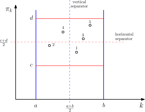
Figure 4: This sketch depicts the notion of vertical and horizontal global separators. In this example, the vertical dashed (blue) line is a vertical separator, splitting the range $[a,b]$ into two equal-sized halves. The horizontal dashed (red) line is a horizontal separator. The example also shows a $(24135)$ copy. This copy is counted only if (i) the “2” is to the left and the “5” is to the right of the vertical separator, and, (ii) if the “1” is below and the “5” is above the horizontal separator.

In addition to vertical separators, we introduce horizontal separators that further partition each $v$ based on the $y$-axis. This second layer of separation divides the region into four distinct quadrants. We refer to Figure 8 for an illustration. In addition, we consider all valid configurations of $24135$ copies relative to these quadrants. For instance, we can enforce that specific elements (e.g., “2” and “5”) fall on opposite sides of the vertical separator and that others (e.g., “1” and “5”) fall on opposite sides of the horizontal separator. This structure ensures that each copy of the pattern is counted exactly once within a unique configuration. Crucially, it turns out that this structure also induces monotonicity and allows for using the Birgé decomposition for efficient approximate counting.

1.2.4 A Primitive for Counting $12$ Copies within Axis-Parallel Rectangles (Section 5.1)

Our final technique introduces a data structure for counting simple $12$ patterns (increasing pairs) within arbitrary axis-aligned rectangles. This primitive allows us to query the approximate number of $12$ copies within any subregion of the input permutation. We employ this data structure to count $5$-patterns.

To develop this $12$-copy counting data structure, we employ a two-dimensional segment tree described in the previous subsection. With this tree, we pre-process the points in a bottom-up manner in $O(n\cdot\mathrm{poly}(\log n,\varepsilon^{-1}))$ time. Section 5.1 details the implementation of this bottom-up pre-processing. This pre-processing computes an approximate number of $12$ copies within each vertex of the segment tree. These pre-computed values are later used to answer queries for approximating the number of $12$ copies within arbitrary rectangles, each answered in polylogarithmic time.

1.3 Open problems

Our results and techniques open several interesting follow-up questions, both as the first approximate counting results for $k>2$ and due to the novel use of the Birgé decomposition.

The main open question is on the complexity of approximate counting for general (small) $k$. As discussed, there are complexity separations between detection and exact counting of permutation patterns: detection takes $O(n)$ time for any fixed length $k$, while exact counting requires $n^{1+\Omega(1)}$ time for $k=4$, assuming Strong 3-SUM, and $n^{\Omega(k/\log k)}$ time when $k$ is a parameter, assuming ETH. Approximate counting lies between exact counting and detection, and it is a priori unclear where its complexity sits between linear in $n$ (for detection) and nearly worst-possible (for exact counting).

Question 1.3 (Complexity of approximate counting).

What is the time complexity of approximating the number of $\sigma$-patterns in an input sequence $f\colon[n]\to{\mathbb{R}}$ to within a $(1+\epsilon)$-multiplicative error, as a function of $n$ and $k=|\sigma|$?

Establishing tight upper and lower bounds for 1.3 appears to be challenging. Even for exact pattern counting, a more extensively studied problem, there remains a gap between the best known upper bound of $n^{k/4+o(k)}$ and the conditional lower bound of $n^{\Omega(k/\log k)}$, both attained by Berendsohn, Kozma and Marx [BKM21]. Nevertheless, given the separation we establish for $k=4$ and $k=5$ (along with the new techniques which are specially suited for approximate computation) it is tempting to conjecture that the complexity of approximate counting in the general case, as a function of $n$ and $k$, is fundamentally lower than that of exact counting. We make the following conjecture.

Conjecture 1.4.

The time complexity of approximate counting $\sigma$-copies in a length-$n$ sequence, as a function of $n$ and $k=|\sigma|$, is asymptotically smaller than that of exact counting for the same parameters.

Proving any bound of the form $n^{o(k/\log k)}$ would affirm this conjecture. But even improving upon the state of the art for exact counting would be interesting. The current best known approach of [BKM21] formulates the pattern matching instance as a constraint satisfaction problem (CSP) with binary constraints. The complexity of solving this CSP is $O(n^{t+1})$, where $t$ is the treewidth of the incidence graph of the pattern $\pi$ (see also the work of Ahal and Rabinovich [AR08] for an earlier investigation of the role of treewidth in this context). The basic constraint graph has treewidth bounded by $k/3+o(k)$; Berendsohn et al. combine the tree-width based approach with a gridding technique based on ideas of Cygan, Kowalik, and Socała [CKS19] to reduce the exponent to $k/4+o(k)$.

As we see here, algorithmic results for both detection and exact counting make use of central width notions from the parametrized complexity literature: the former gave rise to twin-width [GM14, BKTW21] and the latter makes heavy use of tree-width [AR08, BKM21]. It would be very intriguing to explore what role such width notions may play in the approximate version of pattern counting. The fact that approximate counting (in the small $k$ case) admits techniques that go beyond the exact case may suggest that either a complexity notion other than tree-width is at play here, or we can use the new techniques to bound the tree-width of an easier subproblem (with more of the values constrained due to the use of, say, substructure monotonicity and Birgé approximation).

From the lower bound side, essentially no nontrivial (superlinear) results are known for the Word RAM model, and proving any $\omega(n)$ lower bound that applies to the approximate counting of some fixed-length patterns would be interesting. We further conjecture that for large enough (constant) $k$, there should be a strongly superlinear bound.

Conjecture 1.5.

There exists a pattern $\sigma$ of constant length for which approximate counting of $\sigma$ in length-$n$ sequences requires $n^{1+\Omega(1)}$ time.

For $k=3,4,5$, the existing algorithms for, say, 2-approximate counting (and exact counting, for $k=3$) have time complexity $n\log^{O(1)}n$. This raises the question of whether the polylogarithmic dependence is necessary (for $k=2$ it is not necessary [CP10]). We conjecture that the answer is positive already for $k=4$.

Finally, the use of Birgé decomposition in this paper seems to be novel in the context of pattern counting and, perhaps more generally, in combinatorial contexts beyond the scope of distribution testing. This decomposition is very useful in our setting as many sequences of quantities turn out to be monotone. It would be interesting to find other counting problems in low-dimensional geometric settings where this technique, of finding and exploiting monotone subsequences, may be useful.

2 Preliminaries

2.1 Algorithmic primitives

2.1.1 Segment trees

We use a natural and standard representation of permutations in which a permutation $\pi$ is represented by a set of points $\{(i,\pi_{i}):i\in[n]\}$ in plane. On this set of points, our algorithms perform simple counting queries.

Lemma 2.1 (Segment tree data structure).

Let $\pi$ be a permutation over $[n]$. Define

$$S_{i,j}^{a,b}:=|\{x\in[n]:i\leq x\leq j,a\leq\pi(x)\leq b\}|.$$

and $N_{i,j}^{a,b}=|S_{i,j}^{a,b}|$. There exists a data structure that, given $\pi$, initializes in time $O(n\log^{2}n)$ using $O(n\log n)$ space, and supports the following operations in time $O(\log^{2}n)$:

1. Value and location counts: given indices $i\leq j\in[n]$ and values $a\leq b\in[n]$, return $N_{i,j}^{a,b}$.

2. Query access to locations in segment: Given $i,j,a,b$ as above, and $1\leq\ell\leq N_{i,j}^{a,b}$, return the index of the $\ell$-th leftmost element within the set $S_{i,j}^{a,b}$.

3. Query access to values in segment: Given $i,j,a,b$ as above, and $1\leq\ell\leq N_{i,j}^{a,b}$, return the $\ell$-th largest value within the set $\{\pi(x):x\in S_{i,j}^{a,b}\}$.

Lemma 2.1 can be obtained using standard techniques in the data structure literature. For completeness, we outline those techniques in Appendix A.

2.1.2 Birgé decomposition: Fast approximation of monotone sums

One of the central technical tools we use is a slight variant on a classical result of Birgé [Bir87]. The result asserts that one can approximate the sum of a monotone sequence accurately by querying only logarithmically many elements from the sequence in an oblivious manner (that does not depend on their values). To present the result formally, we need the notion of an oblivious decomposition of $[n]$ into intervals.

Definition 2.2 (Oblivious decomposition [Can20, Definition D.14]).

Given a parameter $\varepsilon>0$ and $n\in{\mathbb{N}}$, the $(\varepsilon,{\mathbb{N}})$-oblivious decomposition $\mathcal{J}_{\varepsilon}(n)=\{I_{1},\ldots,I_{\ell}\}$ is a decomposition of $[n]$ into $\ell=\Theta(\epsilon^{-1}\cdot\log n)$ intervals satisfying $|I_{t}|=\lfloor(1+\varepsilon)^{t}\rfloor$ for $1\leq t<\ell$, and $I_{\ell}\leq\lfloor(1+\varepsilon)^{\ell}\rfloor$.

The main technical lemma that we prove is presented next.

Lemma 2.3 (Birgé-type lemma for monotone sums).

Fix a positive parameter $\varepsilon\in{\mathbb{R}}$, let $n\in{\mathbb{N}}$, write $\ell=|\mathcal{J}_{\varepsilon}(n)|$, and let $i_{1}<i_{2}<\ldots<i_{\ell}\in[n]$ be a collection of indices so that each interval $I_{j}\in\mathcal{J}_{\varepsilon}(n)$ contains exactly one index, $i_{j}$. Let $x_{1}\geq x_{2}\geq\ldots\geq x_{n}$ be any monotone non-increasing set of non-negative real numbers. Then

$$\sum_{j=1}^{\ell}x_{i_{j}}\cdot|I_{j}|=(1\pm O(\varepsilon))\sum_{i=1}^{n}x_{i}.$$

As an immediate application, since the sizes of the intervals $I_{j}$ are known in advance, approximating the sum $\sum_{i=1}^{n}x_{i}$ to within a $1\pm\varepsilon$ multiplicative factor can be done in $O(\log n/\varepsilon)$ time (assuming that accessing the value of each $x_{i}$ requires $O(1)$ time). This is summarized in the following lemma.

Lemma 2.4 (Fast approximation of monotone sums).

Let $0<\varepsilon<1$ and $n\in{\mathbb{N}}$ be known parameters, and suppose we are given query access to a monotone sequence $x_{1}\geq x_{2}\geq\ldots\geq x_{n}\geq 0$ of real numbers. Then there exists a deterministic algorithm which returns a value $y\in(1\pm\varepsilon)\sum_{i=1}^{n}x_{i}$, with query complexity and running time $O(\varepsilon^{-1}\log n)$.

Moreover, if the query access provides a multiplicative $1\pm\gamma$ approximation, then this algorithm returns a value $y\in(1\pm\gamma)(1\pm\varepsilon)\sum_{i=1}^{n}x_{i}$; the algorithm is oblivious to the value of $\gamma$.

We note that this lemma and its proof are slightly different from the statement usually named after Birgé. The traditional version concerns distributions and is often used in distribution testing settings [Can20, DDS⁺13, DDS14]. It assumes that we can approximate the probability density of sub-intervals of elements, which cannot directly be done in our setting. In contrast, our version has a different, query-based access to the input. We also note that the dependence in the proximity parameter $\varepsilon$ for our application is inversely linear, whereas for tasks such as learning monotone distributions, the optimal dependence is known to be polynomial (and superlinear) in $1/\varepsilon$.

Proof of Lemma 2.3.

Write $\mathcal{J}_{\varepsilon}(n)=\{I_{1},\ldots,I_{\ell}\}$ using the same notation as in Definition 2.2. For each interval $I_{j}$, let $m_{j}=\min(I_{j})$ and $M_{j}=\max(I_{j})$. by the monotonicity of the sequence $(x_{i})_{i=1}^{n}$, we know that

$$\sum_{j=1}^{\ell}x_{m_{j}}\cdot|I_{j}|\geq\sum_{j=1}^{\ell}x_{i_{j}}\cdot|I_{j}|\geq\sum_{j=1}^{\ell}x_{M_{j}}\cdot|I_{j}|$$

for any choice of indices $i_{j}$ in the statement of the lemma. Indeed, this is true since $x_{m_{j}}\geq x_{i_{j}}\geq x_{M_{j}}$ due to the monotonicity. Next, note that we also have

$$\sum_{j=1}^{\ell}x_{m_{j}}\cdot|I_{j}|\geq\sum_{i=1}^{n}x_{i}\geq\sum_{j=1}^{\ell}x_{M_{j}}\cdot|I_{j}|,$$

since for each $j$, $x_{m_{j}}|I_{j}|\geq\sum_{i\in I_{j}}x_{i}\geq x_{M_{j}}|I_{j}|$, again from the monotonicity. Thus, to complete the proof of the lemma, it remains to prove the following inequality:

$$\sum_{j=1}^{\ell}x_{m_{j}}|I_{j}|\leq(1+O(\varepsilon))\cdot\sum_{j=1}^{\ell}x_{M_{j}}|I_{j}|.$$ (1)

The rest of the proof is dedicated to establishing (1).

For simplicity, we may assume that $1/\varepsilon$ is an integer. For each integer $1\leq t\leq 1/\varepsilon$, define

$$A_{t}=\{j\in[\ell]:|I_{j}|=t\},\qquad\qquad j^{(t)}=\max A_{t},\qquad\qquad i_{t}=M_{j^{(t)}}=\max I_{j^{(t)}}.$$

Note that the following hold with respect to $A_{t}$, $j^{(t)}$, and $i_{t}$:

• $A_{t}$ is a contiguous interval in $[\ell]$, i.e., each $A_{t}$ is a subset of the form $\{j^{(t-1)}+1,j^{(t-1)}+2,\ldots,j^{(t)}\}$. Moreover, $1\in A_{1}$, and all elements of $A_{t}$ are smaller than all elements of $A_{t^{\prime}}$ for $t^{\prime}>t$.

• $|I_{j^{(t)}+1}|=|I_{j^{(t)}}|+1$ for all $t$.

• $i_{t}$ is the maximum index of an element that belongs to an interval of length $t$ in the oblivious decomposition.

Also define $A^{\prime}=[\ell]\setminus\bigcup_{t=1}^{1/\varepsilon}A_{t}$. By definition, we can write the difference between the sums on the left and right hand sides of (1) as follows:

$$\sum_{j=1}^{\ell}x_{m_{j}}|I_{j}|-\sum_{j=1}^{\ell}x_{M_{j}}|I_{j}|=\sum_{t=1}^{1/\varepsilon}\left(t\cdot\sum_{j\in A_{t}}(x_{m_{j}}-x_{M_{j}})\right)+\sum_{j\in A^{\prime}}|I_{j}|\cdot(x_{m_{j}}-x_{M_{j}}).$$ (2)

Now, the summand corresponding to $t=1$ in (2) is equal to zero, since $m_{j}=M_{j}$ when $|I_{j}|=1$. For $2\leq t\leq 1/\varepsilon$, we have

$$\sum_{j\in A_{t}}(x_{m_{j}}-x_{M_{j}})\leq\sum_{j\in A_{t}}(x_{M_{j-1}}-x_{M_{j}})=x_{i_{t-1}}-x_{i_{t}},$$

and so the first sum in the right hand side of (2) is bounded by

$$x_{i_{1}}-\frac{1}{\varepsilon}\cdot x_{i_{1/\varepsilon}}+\sum_{t=1}^{1/\varepsilon}x_{i_{t}}.$$

We next claim that

$$x_{i_{1}}+\sum_{t=1}^{1/\varepsilon}x_{i_{t}}\leq O(\varepsilon)\cdot\sum_{i=1}^{i_{1/\varepsilon}}x_{i}.$$

Indeed, this follows by observing that for each $1\leq t\leq 1/\varepsilon$, we have $i_{t+1}-i_{t}=\Theta(1/\varepsilon)$, and the fact that $x_{i}\geq x_{i_{t}}$ for all $i\in\bigcup_{I\in A_{t}}I$. Now, for any $j$ where $I_{j}\in\mathcal{A}^{\prime}$, we have that $|I_{j+1}|\leq(1+O(\varepsilon))|I_{j}|$. Thus, by a telescopic sum argument, we conclude that

$$\sum_{j\in A^{\prime}}x_{m_{j}}|I_{j}|\leq\sum_{j\in A^{\prime}}x_{M_{j-1}}|I_{j}|\leq x_{i_{1/\varepsilon}}|I_{j^{(1/\varepsilon)}+1}|+(1+O(\varepsilon))\cdot\sum_{j=j_{0}}^{\ell}x_{M_{j}}|I_{j}|$$ (3)

where we recall that $|I_{j^{(1/\varepsilon)}+1}|=\frac{1}{\varepsilon}+1$. Combining all of the above inequalities, we have that

$$\sum_{j=1}^{\ell}x_{m_{j}}|I_{j}|-\sum_{j=1}^{\ell}x_{M_{j}}|I_{j}|\leq O(\varepsilon)\cdot\sum_{j=1}^{\ell}x_{M_{j}}|I_{j}|,$$

which establishes (1). ∎

3 Almost all $4$-length patterns via Birgé

3.1 Symmetry reductions and known results

It is folklore that patterns form certain equivalency groups. For instance, counting $1234$ copies is equivalent to counting $4321$: the number of $4321$ copies in a sequence $\pi$ is the same as that of $1234$ copies in the reverse of $\pi$ (i.e., in $\pi$ reflected along a vertical axis). Similarly, counting $2134$ copies is equivalent to counting $3421$, as the number of $3421$ copies in a sequence $\pi$ is the same as the number of $2134$ copies in the sequence in which the $i$-th element equals $n+1-\pi_{i}$ (i.e., in the sequence reflected along a horizontal axis).

Moreover, it has been established that copies of some of these $8$ patterns can be counted in near-linear time, even exactly.

Theorem 3.1 ([EZL21]).

The occurrences of copies $1234$, $1243$, and $2143$ in a given permutation can be counted in time $\tilde{O}(n)$.

In this work, our goal is to show that the remaining $4$-length copies can be approximately counted also in near-linear time. It turns out that the remaining non-symmetric ones, i.e., $1324$, $1342$, $1423$, $1432$, and $2413$, can be split into two categories based on their properties. In this section, we describe an idea that enables us to approximately count the number of copies of $1324$, $1342$, $1423$, and $1432$. To handle $2413$, we in detail introduce an additional idea in Section 4.

3.2 Approximately counting $1324$ copies

In this section, we describe how to approximately count $1324$ copies and then extend that to $1342,1423$, and $1432$; see Section 3.3. Fix a permutation $\pi$, let $\mathcal{C}$ be all $1324$ copies in $\pi$. The underlying idea of our approach is to partition $\mathcal{C}$ into classes so that it is relatively easy to approximate the size of each class.

3.2.1 Fixing “$3$” in $1324$ copies

As the first step, our approach partitions $\mathcal{C}$ with respect to the value of the “$3$”. In particular, there are $n$ such classes $\mathcal{C}_{1},\mathcal{C}_{2},\ldots,\mathcal{C}_{n}$ such that $\mathcal{C}_{i}$ is the subset of $\mathcal{C}$ with their $3$-value being equal $\pi_{i}$. Clearly,

$$|\mathcal{C}|=\sum_{i=1}^{n}|\mathcal{C}_{i}|.$$

Our approach approximates each $|\mathcal{C}_{i}|$ independently. The main technical contribution of our work is showing that $\mathcal{C}_{i}$ can be further partitioned into classes that exhibit certain monotonicity in their size. Our approach employs Birgé decomposition, e.g., Lemma 2.3, to leverage that property and approximate $|\mathcal{C}_{i}|$ in only $\mathrm{poly}\log n$ time. We now describe the details of this idea.

3.2.2 Monotonicity with respect to “$4$” within $\mathcal{C}_{i}$

Consider the example in which $\pi=136548279$, as illustrated in Figure 2. Fix $6$ to be “3” in a $1324$ copy. In that case, the candidates for “4” are $8,7$, and $9$. Since $7$ and $9$ appear in $\pi$ after $8$, any $1324$ copy of the form $\pi_{x}6\pi_{y}8$ also yields $1324$ copies $\pi_{x}6\pi_{y}7$ and $\pi_{x}6\pi_{y}9$. We formalize this observation as follows.

Lemma 3.2.

Let $\mathcal{C}_{i}$ be the set of all $1324$ copies of a permutation $\pi$ such that “3” equals $\pi_{i}$. Let $\mathcal{C}_{i,j}$ be the set of all $1324$ copies such that $\pi_{x}\pi_{i}\pi_{y}\pi_{j}\in\mathcal{C}_{i}$. Then, $|\mathcal{C}_{i,j}|\leq|\mathcal{C}_{i,j^{\prime}}|$ for each $i<j<j^{\prime}$ with $\pi_{i}<\pi_{j},\pi_{j^{\prime}}$.

Proof.

Let $\pi_{x}\pi_{i}\pi_{y}\pi_{j}\in\mathcal{C}_{i,j}$. By the fact that we consider $1324$ copies, it implies $\pi_{x}<\pi_{i}$, $\pi_{y}<\pi_{i}$ and $y<j$. Since $\pi_{i}<\pi_{j}$, $\pi_{i}<\pi_{j^{\prime}}$ and $j<j^{\prime}$, we have that $\pi_{x}\pi_{i}\pi_{y}\pi_{j^{\prime}}\in\mathcal{C}_{i,j^{\prime}}$. ∎

Lemma 3.2 essentially states that $\mathcal{C}_{i}$ can be partitioned into subsets $\mathcal{C}_{i,j}$ whose sizes are non-decreasing when ordered with respect to $j$ – the claim excludes $\mathcal{C}_{i,j}$ for which $\pi_{j}\leq\pi_{i}$; for such cases $\mathcal{C}_{i,j}=\emptyset$ anyway. By Lemma 2.4, this further implies that to approximate $|\mathcal{C}_{i}|$, it suffices to (approximately) compute $|\mathcal{C}_{i,j}|$ for only $O(\log n/\varepsilon)$ different values of $j$ with $\pi_{j}>\pi_{i}$ and $j>i$. Our next goal is to discuss how to compute an approximation of $|\mathcal{C}_{i,j}|$.

3.2.3 Monotonicity with respect to “$2$” within $\mathcal{C}_{i,j}$

Recall that $\mathcal{C}_{i,j}$ corresponds to all $1324$ copies with “3” being $\pi_{i}$ and “4” being $\pi_{j}$. As before, consider the example in which $\pi=136548279$, as illustrated in Figure 5. Fix $6$ to be “3” and $9$ to be “4” in a $1324$ copy. In that case, the candidates for “2” are $2,4$, and $5$. Since $4>2$ and $5>2$, any $1324$ copy of the form $\pi_{x}629$ also yields $1324$ copies $\pi_{x}649$ and $\pi_{x}659$. We formalize this observation as follows.

Figure 5: The illustration corresponds to permutation $\pi=136548279$, depicted in a plane at points $(i,\pi_{i})$.

Lemma 3.3.

Let $\mathcal{C}_{i.j}$ be the set of all $1324$ copies of a permutation $\pi$ such that “3” equals $\pi_{i}$ and “4” equals $\pi_{j}$. Let $\mathcal{C}_{i,j,k}$ be the set of all $1324$ copies such that $\pi_{x}\pi_{i}\pi_{k}\pi_{j}\in\mathcal{C}_{i,j}$. Then, $|\mathcal{C}_{i,j,k}|\leq|\mathcal{C}_{i,j,k^{\prime}}|$ for each $\pi_{k}<\pi_{k^{\prime}}$ with $i<k<j$, $i<k^{\prime}<j$ and $\pi_{k},\pi_{k^{\prime}}<\pi_{i}$.

Proof.

Let $\pi_{x}\pi_{i}\pi_{k}\pi_{j}\in\mathcal{C}_{i,j,k}$. By the fact that we consider $1324$ copies, it implies $\pi_{x}<\pi_{k}$ and $x<i<k$. Since $\pi_{k}<\pi_{k^{\prime}}<\pi_{i}$ and $i<k^{\prime}<j$, we have that $\pi_{x}\pi_{i}\pi_{k^{\prime}}\pi_{j}\in\mathcal{C}_{i,j,k^{\prime}}$. ∎

Lemma 3.3 states that $\mathcal{C}_{i,j}$ can be partitioned into subsets $\mathcal{C}_{i,j,k}$ whose sizes are non-decreasing when ordered with respect to $\pi_{k}$. By Lemma 2.4, this further implies that to approximate $|\mathcal{C}_{i,j}|$, it suffices to (approximately) compute $|\mathcal{C}_{i,j,k}|$ for only $O(\log n/\varepsilon)$ different values of $k$ with $i<k<j$ and $\pi_{k}<\pi_{i}$. Coupling this with Lemma 3.2, $|\mathcal{C}_{i}|$ can be approximate by computing $|\mathcal{C}_{i,j,k}|$ for only $\mathrm{poly}(\log{(n)}/\varepsilon)$ different pairs of $j$ and $k$.

3.2.4 Algorithm

As a reminder, $\mathcal{C}_{i,j,k}$ is the set of all $1324$ copies such that “3” equals $\pi_{i}$, “4” equals $\pi_{j}$, and “2” equals $\pi_{k}$. $|\mathcal{C}_{i,j,k}|$ is computed by counting the number of points $(\ell,\pi_{\ell})$ such that $1\leq\ell\leq i-1$ and $1\leq\pi_{\ell}<\pi_{k}-1$. This can be done in $\mathrm{poly}\log n$ time using sparse segment trees, as provided by Lemma 2.1. This now enables us to provide the pseudo-code of our approach (Algorithm 1).

1:Input: A permutation $\pi$; an approximation parameter $\varepsilon>0$

2:Output: a $1+\varepsilon$ approximation of the number of $1324$ copies in $\pi$

3: 

4:Build a sparse segment tree $S$ on $(i,\pi_{i})$ for all $i=1\ldots n$

5:for $i=1\ldots n$ $\triangleright$ Fix “3” do

6:     Let $J$ be the set of candidates for “4” in 1324 copies given that “3” is fixed to $\pi_{i}$.

7:     Let $J^{\prime}$ be the subset of $J$ queried by the algorithm in Lemma 2.4.

8:     for $j\in J^{\prime}$ $\triangleright$ Fix “4” do

9:         Let $K$ be the set of candidates for “2” in 1324 copies given that “3” is fixed to $\pi_{i}$ and “4” is fixed to $\pi_{j}$.

10:         Let $K^{\prime}$ be the subset of $K$ queried by the algorithm in Lemma 2.4.

11:         for $k\in K^{\prime}$ $\triangleright$ Fix “2” do

12:              Let $c_{i,j,k}$ be the number of points $(x,\pi_{x})$ in $S$ such that $x\leq i-1$ and $\pi_{x}\leq\pi_{k}-1$.          

13:         Use the algorithm from Lemma 2.4 to output a $1\pm\varepsilon$ approximation of $|\mathcal{C}_{i,j}|$ by using $c_{i,j,k}$ as the query points. Denote that approximation by $c_{i,j}$.      

14:     Use the algorithm from Lemma 2.4 to output a $1\pm\varepsilon$ approximation of $|\mathcal{C}_{i}|$ by using $c_{i,j}$ as the query points. Denote that approximation by $c_{i}$.

15:return $\sum_{i=1}^{n}c_{i}$

Algorithm 1 Approximate-1324-Copies

We are now ready to show the following.

Theorem 3.4.

Given a permutation $\pi$ and an approximation parameter $\varepsilon\in(0,1)$, Algorithm 1 computes a $1\pm 3\varepsilon$ approximation of the number of $1324$ copies in $\pi$ in time $O(n\cdot\mathrm{poly}(\log(n)/\varepsilon))$.

Proof.

We analyze separately the running time and the approximation guarantee.

Running time.

There are $n$ options to choose $i$. By Lemma 2.4, $|J^{\prime}|,|K^{\prime}|\in O(\log(n)/\varepsilon)$. Note that the sets $J$ and $K$ need not be constructed explicitly. It suffices to, for a given $t$, be able to access the $t$-th element of those sets, which can be done in $O(\log^{2}n)$ time using $S$. Finally, 12 of Algorithm 1 can be executed in $O(\log^{2}n)$ time; see Lemma 2.1.

Therefore, the overall running time is $O(n\cdot\mathrm{poly}(\log(n)/\varepsilon))$.

Approximation guarantee.

Let $c_{i,j,k}$, $c_{i,j}$ and $c_{i}$ be as defined in Algorithm 1. Observe that $c_{i,j,k}=|\mathcal{C}_{i,j,k}|$. By the guarantee of the algorithm in Lemma 2.4, we have $c_{i,j}\in(1\pm\varepsilon)|\mathcal{C}_{i,j}|$.

Since $c_{i,j}$ are used to obtain an approximation $c_{i}$ of $|\mathcal{C}_{i}|$, by Lemma 2.4 we have that $c_{i}\in(1\pm\varepsilon)(1\pm\varepsilon)|\mathcal{C}_{i}|\in(1\pm 3\varepsilon)|\mathcal{C}_{i}|$, for $\varepsilon\in(0,1)$. ∎

3.3 Approximately counting $1342,1423$ and $1432$ copies

Our algorithm to approximately count $1324$ copies can be described as follows: Fix “3”; then, “4” counts are position-monotone; then, “2” counts are value-monotone. In the same way can be described the algorithms for approximately counting copies $1342,1423$, and $1432$. We provide those descriptions below, and the formal proofs follow exactly the same lines as for $1324$ copies.

1. Fix “3”; then, “4” counts are position-monotone; then, “2” counts are value-monotone.

2. Fix “2”; then, “3” counts are value-monotone; then, “4” counts are position-monotone.

3. Fix “3”; then, “2” counts are value-monotone; then, “4” counts are position-monotone.

4 Handling $2413$ copies via Birgé and Separators

The main idea behind approximate counting of $1324$ copies was to fix one of the positions and then show that the counts are monotone with respect to two other positions, e.g., fix “3”, then the counts are monotone with respect to the position of “4”; after fixing “3” and “4”, the counts are monotone with respect to the value of “2”. Unfortunately, copies of $2413$ do not seem to exhibit such a property. To alleviate that, we observe that there is an additional way of partitioning the copies of $2413$.

To illustrate this partitioning approach, assume that we fix “4”. Then, we would like to exhibit the monotonicity of the copy counts with respect to the value or position of at least one among “2”, “1”, and “3”. However, this is not the case. Intuitively, the challenge here is that the tools we developed so far do not enable us to approximate the number of copies of $12$ in a given permutation in $\mathrm{poly}(\log n,1/\varepsilon)$ time. To see how it affects counting $2413$ copies, for instance, after fixing a “4”, no special structure is imposed on the candidates of “1” and “3”! Indeed, even though both “1” and “3” have to be to the right and below the fixed “4”, our algorithm still needs to (approximately) count the number of monotone pairs in a given subarray.

What if we are concerned only with the number of $2413$ copies in which the position of “1” is less than $s$, while the position of “3” is greater than $s$? This situation is illustrated in Figure 3, and $s$ should be thought of as “separator”. After imposing this additional structure between “1” and “3”, the counts become monotone with respect to the value of “3”. Hence, we can again apply the Birgé theorem for approximating the counts.

It remains to show that there exists a small number of separators that enable counting all $2413$ copies. We dive into those details in the rest of this section, describing how to partition “3” and “4” into certain buckets that allow for the described $2413$-copy partitioning. Ultimately, this section leads the following result:

Theorem 4.1 (Approximating $2413$ copies).

There exists a deterministic algorithm for approximating the number of $2413$ copies in a permutation of length $n$ to within a multiplicative factor of $1+\varepsilon$, with running time of $n\cdot\mathrm{poly}(\log n,1/\varepsilon)$.

Organization of this section.

We begin by, in Section 4.1, stating several definitions that are instrumental in describing our partitioning of $2413$. Section 4.2 outlines our proof of Theorem 4.1, while Sections 4.3 and 4.4 prove the main technical claims we need in the proof of Theorem 4.1.

4.1 Preliminaries

For convenience, we let $[n]:=\{0,1,\ldots,n-1\}$. We begin by defining the notion of $j$-buckets and type-$j$ copies, which are instrumental in defining the kind of separator we use and illustrate in Figure 3. Recall that a copy of $2413$ in a permutation $\pi\colon[n]\to[n]$ is any quadruple of indices $i_{1}<i_{2}<i_{3}<i_{4}$ such that $\pi(i_{3})<\pi(i_{1})<\pi(i_{4})<\pi(i_{2})$.

Definition 4.2 (Type of copy; $j$-buckets).

For each index $i\in[n]$ consider the standard binary representation of $i$ using $\lceil\log n\rceil$ bits, and define the $j$-least significant bit (or $j$-LSB in short) as the term corresponding to $2^{j}$ in the binary representation. We say that a $2413$ copy $(i_{1},i_{2},i_{3},i_{4})$ in $\pi$ is type-$j$ if $i_{2}$, i.e., the index of the “4”, and $i_{4}$ (the index of the “3”) differ on the $j$-LSB, but have equal $j^{\prime}$-LSB for all $j^{\prime}>j$.

Finally, two indices in $[n]$ are said to be in the same $j$-bucket if their $j^{\prime}$-LSB is equal for all $j^{\prime}\geq j$. This definition is illustrated in Figure 6.

Observe that there are many $j$-buckets. In fact, $j$-buckets partition the integers into sets of $2^{j}$ consecutive integers each. For instance, the ranges of integers $[0,7]$, $[8,15]$, $[16,23]$, $[24,31]$ are all $3$-buckets.

Figure 6: This example depicts a copy of $2413$ equal to $(2,6,7,14)$ with $\pi(i_{1})=8$, $\pi(i_{2})=12$, $\pi(i_{3})=6$ and $\pi(i_{4})=9$. Since $i_{2}=(00110)_{2}$ and $i_{4}=(01110)_{2}$, this copy is $3$-type. Moreover, we have that all $i_{1},i_{2},i_{3}$ and $i_{4}$ are in the same $4$-bucket. The indices $i_{1},i_{2}$ and $i_{3}$ are in the same $3$-bucket as well, while $i_{2}$ and $i_{3}$ are in addition in the same $2$-type and $1$-type bucket; see Definition 4.2.

Note that a bucket consists of contiguous subintervals of $[n]$. Moreover, in a $2413$ copy which is type-$j$, the “4” and “2” are in the same $(j+1)$-bucket and in different, but neighboring, $j$-buckets. This motivates the following definition.

Definition 4.3 ($4$-heavy, $3$-heavy).

Consider a type-$j$ $2413$ copy $(i_{1},i_{2},i_{3},i_{4})$. We say that the copy is $4$-heavy if $i_{2}$ and $i_{3}$, i.e., the “4” and “1”, are in the same $j$-bucket. Otherwise, we say that the copy is $3$-heavy.

Note that in a type-$j$ copy $(i_{1},i_{2},i_{3},i_{4})$ that is $3$-heavy, $i_{3}$ (“the $1$-entry”) is in the same $j$-bucket as $i_{4}$ (“the $3$-entry”). Similarly, in a type-$j$ copy $(i_{1},i_{2},i_{3},i_{4})$ that is $4$-heavy, $i_{3}$ (“the $1$-entry”) is in the same $j$-bucket as $i_{2}$ (“the $4$-entry”). This yields the following observation.

Observation 4.4.

Each type-$j$ copy is either $3$- or $4$-heavy, but not both.

4.2 Proof of the main theorem

The proof of the main result of this section, i.e., Theorem 4.1, relies on the following two claims saying that the count of $3$- and $4$-heavy copies of a fixed type can be approximated in nearly linear time.

Lemma 4.5 (Approximation of $4$-heavy copies).

Let $n\in\mathbb{N}$, $i\in[n]$, and $j\in\left[\left\lceil\log n\right\rceil\right]$. Let $S$ be a pre-built segment tree for $\{(i,\pi_{i}):i\in[n]\}$. There exists a deterministic algorithm with running time $\mathrm{poly}(\log n,\varepsilon)$ that, given access to $S$, returns a $(1+\varepsilon)$-approximation of the number of $4$-heavy type-$j$ copies $(i_{1},i_{2},i_{3},i_{4})$ of $(2413)$ in $\pi$ for which $i_{2}=i$.

Lemma 4.6 (Approximation of $3$-heavy copies).

Let $n\in\mathbb{N}$, $i\in[n]$, and $j\in\left[\left\lceil\log n\right\rceil\right]$. Let $S$ be a pre-built segment tree for $\{(i,\pi_{i}):i\in[n]\}$. There exists a deterministic algorithm with running time $\mathrm{poly}(\log n,\varepsilon)$ that, given access to $S$, returns a $(1+\varepsilon)$-approximation of the number of $3$-heavy type-$j$ copies $(i_{1},i_{2},i_{3},i_{4})$ of $(2413)$ in $\pi$ for which $i_{4}=i$.

With Lemmas 4.5 and 4.6 in hand, the proof of Theorem 4.1 is almost immediate.

Proof of Theorem 4.1.

Our main algorithm is given as Algorithm 2.

1:Input: A permutation $\pi$; an approximation parameter $\varepsilon>0$

2:Output: A $1+\varepsilon$ approximation of the number of $2413$ copies in $\pi$

3: 

4:Build a segment tree $S$ on $(i,\pi_{i})$ for all $i=1\ldots n$ as described in Appendix A.

5:for $i=0\ldots n-1$ do

6:     for $j=0\ldots\lceil\log n\rceil$ do

7:         Compute the approximate count $C_{j,4,i}$ of type-$j$ $4$-heavy copies of $(2413)$ whose $4$-entry is at location $i$, using the algorithm of Lemma 4.5 and passing $S$ to it.

8:         Compute the approximate count $C_{j,3,i}$ of type $j$ $3$-heavy copies of $(2413)$ whose $3$-entry is at location $i$, using the algorithm of Lemma 4.6 and passing $S$ to it.      

9:return $\sum_{i,j}(C_{j,3,i}+C_{j,4,i})$

Algorithm 2 Approximate-2413-Copies

Each copy of $(2413)$ in $\pi$ is type-$j$ for exactly one value of $j$, and moreover, each such copy is either $3$-heavy or $4$-heavy, but not both. Hence, the sum $\sum_{i,j}(C_{j,3,i}+C_{j,4,i})$ is a $(1+\varepsilon)$-approximation of the number of $(2413)$-copies in $\pi$.

Since $S$ can be built in $\tilde{O}(n)$ time, and each invocation to the algorithms from Lemmas 4.5 and 4.6 takes $\mathrm{poly}(\log n,1/\varepsilon)$ time, Algorithm 2 runs in $\tilde{O}\left(n\cdot\mathrm{poly}(1/\varepsilon)\right)$ time. ∎

It remains to prove Lemma 4.5 and Lemma 4.6. We refer the reader to a (very schematic) illustration for the $4$-heavy case (Lemma 4.5).

4.3 Approximating the number of $4$-heavy copies

Figure 7: A helper illustration for the proof of Lemma 4.5. In this sketch, $t$ is an integer. The shaded rectangle corresponds to the set $X$ of “candidates for $3$”.

Proof of Lemma 4.5.

Fix $j$. Consider the set $A_{i}$ of all $4$-heavy type-$j$ $(2413)$-copies $(i_{1},i_{2},i_{3},i_{4})$ where $i_{2}=i$, i.e., all copies where the “4” is located at index $i$. Recall that these are precisely all copies where the “1” is in the same $j$-bucket as index $i$, whereas the “3” is not in the same bucket. In particular, for any two such copies $(i_{1},i,i_{3},i_{4})$ and $(i^{\prime}_{1},i,i^{\prime}_{3},i^{\prime}_{4})$, it holds that $i^{\prime}_{4}>i_{3}$, i.e., all “3’s” lie to the right of all “1’s”.

“3” candidates.

We approximate $|A_{i}|$ by first fixing the “candidate for $3$”; the “candidate for $4$” is already fixed by the definition of $A_{i}$. Moreover, we show that a particular function is monotone with respect to those candidates, which will enable us to apply Lemma 2.4; we invoke Lemma 2.4 with parameter $\varepsilon/3$. Formally, let $X$ be the set of indices with the following two properties: (1) the indices in the $j$-bucket immediately neighboring to “the right” the $j$-bucket $i$ belongs to, and (2) the indices whose value is smaller than $\pi(i)$. In Figure 7, $X$ corresponds to the shaded area.

For each such candidate $x\in X$, define $f(x)$ as the number of $(2413)$-copies in $A_{i}$. Importantly, $f(x)$ is “monotone by value” within the relevant bucket. Precisely, within $A_{i}$, $f(x)$ is non-decreasing as a function of $\pi(x)$ over $x\in X$. This is easy to see as for $x,x^{\prime}\in X$ such that $\pi(x)>\pi(x^{\prime})$, if $(i_{1},i,i_{3},x^{\prime})$ is a $(2413)$ copy, then $(i_{1},i,i_{3},x)$ is a $(2413)$ copy as well.

Approximating $|A_{i}|$.

By definition, we have that $|A_{i}|=\sum_{x\in X}f(x)$. Moreover, since $f(x)$ is monotone with respect to $\pi(x)$ over $x\in X$, we approximate $\sum_{x\in X}f(x)$ by applying Lemma 2.4. Let $X^{\prime}\subseteq X$ be the subset of size $O(\log n/\varepsilon)$ of indices, and corresponding to Lemma 2.4, for which is needed to (approximately) compute $f(x)$ for $x\in X^{\prime}$. Observe that all the elements in $X$ belong to a well-defined rectangle. Hence, each point in $X^{\prime}$ can be found in $\mathrm{poly}\log n$ time.

Approximating $f(x)$.

Let $x\in X^{\prime}$. Similarly to before, we $f(x)$ in $\mathrm{poly}(\log n,1/\varepsilon)$ time using the segment tree and another application of the Birgé technique.

Indeed, let $S_{x}$ be the set of all $1$-candidates, which are elements between $i$ and the rightmost end of its $j$-bucket, and whose values are less than $\pi(x)$. For each $y\in S$, let $g(y)$ denote the number of $(2413)$-copies of the form $(i_{1},i,y,x)$. Note that $g(y)$ is monotone non-increasing in value. That is, when $\pi(y)$ increases, the number of $(2413)$-copies in $A_{i}$ that $y$ participates in as a “1” can only decrease. Moreover, it is easy to compute $g(y)$ exactly for a specific value of $y$ by invoking a single operation specified by Lemma 2.1. That operation would count all elements that are larger than $\pi(y)$, smaller than $\pi(x)$, and are located to the left of $i$.

Now, because of the monotonicity of $g$, and because $f(x)=\sum_{y\in S_{x}}g(y)$, we apply the Birgé technique (Lemma 2.4) to approximate $f(x)$ for any specific value of $x\in X$ to within a $(1+\varepsilon/3)$-factor using $O(\log n/\varepsilon)$ computations of $g(y)$.

Each of the applications of Birgé introduces a multiplicative error of $1\pm\varepsilon/3$. Provided that $\varepsilon\leq 1/2$, the total multiplicative error is less than $1\pm\varepsilon$. ∎

4.4 Approximating the number of $3$-heavy copies

Proof of Lemma 4.6.

The proof is similar to the one for Lemma 4.5, except that in counting $2413$ copies, the algorithm fixes the “3” but not the “4”. In this proof, we only consider $3$-heavy type-$j$ copies, where the “$1$” is located in the same $j$-bucket as the “$3$”, while the “$4$” is located in a neighboring (to the left) $j$-bucket.

Fix a “3” at location $i$. We consider candidates for “$4$” in the neighboring $j$-bucket – these are all locations $x$ with a value higher than that in location $i$. Among these locations $x$, the count of $2413$ copies with the “4” at $x$ and the “3” at $i$, which are $3$-heavy, is “monotone by location”: it becomes bigger as the index/location $x$ grows in the relevant bucket. This is the case since the possibilities for a “1” remain fixed while moving the “4” to the right allows more options for a “2”. So we apply Birgé for the first time here and only need to compute the approximate count for $O(\log n/\varepsilon)$ specific $x$ locations.

Now, fixing a specific $x$, i.e., specific location of the “$4$”, we proceed exactly as in the proof of Lemma 4.5; this requires another application of Birgé. This completes the analysis ∎

5 All $5$-length patterns via global separators and $12$ copies

This section described the ideas and algorithmic primitives we use to approximately count copies of $5$-patterns. In Section 4, we already described the idea of using a separator to induce additional structure among the copies of a fixed pattern. A part of this section details an extension of those ideas. As a reminder, for pattern $2413$, the idea was first to fix a candidate for the “4” and then find a convenient way to separate the candidates for the “1” and the candidates for the “3” concerning their position. In Section 5.2, we elaborate that it is also possible to first fix a separator and then to fix a candidate for one of the positions in the pattern. In fact, we show that two separators can be fixed before fixing any candidate.

In addition to the separators, we develop a primitive that counts approximately $12$ copies in a given rectangle in only $\mathrm{poly}(\varepsilon^{-1},\log n)$ time. That structure uses $O(n\cdot\mathrm{poly}(\varepsilon^{-1},\log n))$ preprocessing time and is described in length in Section 5.1.

Finally, in Section 5.3 we describe how to combine these ideas and primitives to prove our main result. See 1.1

5.1 Approximately counting $12$ copies within rectangles

In this section, we create a data structure that returns the number of $12$ copies inside an axis-parallel arbitrary rectangle.

Lemma 5.1 (Counting $12$ copies primitive).

There exists a data structure that, given an axis-parallel rectangle $R$ as a query, in $\mathrm{poly}(\log n)\cdot\varepsilon^{-1}$ time outputs a $(1+\varepsilon)$-approximate number of $12$ copies inside $R$. This data structure uses $\tilde{O}(n\varepsilon^{-1})$ pre-computation time.

Note that the existing literature on approximate counting of $12$-copies [AP98, CP10] does not build a data structure as described in Lemma 5.1. While existing work approximates the total count of $12$-copy in only a single box – the whole dataset of $n$ points – our data structure preprocesses the $n$ points once and then allows us to retrieve the (approximate) number of $12$-pairs for arbitrary sub-rectangles we query, in polylogarithmic time. In what follows, we describe how to build this data structure.

Two-dimensional segment tree.

As the starting point, we build a two-dimensional segment tree over the points $(i,\pi_{i})$ over all $i\in[n]$. In Appendix A, we already recall the definition of a segment tree and describe how we use it to count $4$-patterns. For counting $5$-patterns, we build a two-dimensional segment tree as follows:

1. A segment tree $S$ is built over the points $(i,\pi_{i})$ with respect to their $x$-coordinate. We also use outer segment tree to refer to $S$.

2. Consider a vertex $v$ in $S$, and let $[a,b]$ be the interval of the $x$-axis $v$ corresponds to. Then, $v$ stores all the points $(i,\pi_{i})$ such that $a\leq i\leq b$.

3. The points inside each vertex $v$ of $S$ are organized as a segment tree with respect to the $y$-coordinate of the $v$’s points. We call these segment trees inner.

4. Let $v$ be a vertex in the outer and $w$ a vertex in the $v$’s inner segment tree. Let $v$ correspond to $[a,b]$ and $w$ to $[c,d]$. Then, $w$ stores all the points within rectangle $[a,b]\times[c,d]$, i.e., $w$ stores all $(i,\pi_{i})$ such that $a\leq i\leq b$ and $c\leq\pi_{i}\leq d$. Two copies of those points are kept. One copy is sorted with respect to the $x$-coordinates and the other copy is sorted with respect to the $y$-coordinate.

Hence, $S$ is a segment tree of segment trees. The outer segment tree partitions the plane with respect to the $x$-coordinate into recursively nested strips. The inner segment trees partition each of the strips into another family of recursively nested strips but with respect to the $y$-coordinate.

A point $(i,\pi_{i})$ is replicated within $O(\log n)$ vertices in the outer segment tree. Each of those outer vertices replicates $(i,\pi_{i})$ $O(\log n)$ times within its inner segment tree. Hence, a point is replicated $O(\log^{2}n)$ times within $S$.

This conclusion has two implications. First, the points inside the vertices of the inner segment trees can be sorted in $O(n\log^{3}n)$ time. Second, the total number of non-empty vertices across all inner segment trees is $O(n\log^{2}n)$. This is essential as it enables us to build and maintain $S$ in only $\tilde{O}(n)$ time by not creating the vertices that contain no point inside.

Pre-processing 12 copy counts.

Once the two-dimensional segment tree $S$ is built as described, we process its vertices to pre-compute the number of $12$ copies inside each vertex of the inner segment trees. First, we show the following claim.

Lemma 5.2 (12 copies across disjoint useful rectangles).

Given two distinct vertices $w_{1}$ and $w_{2}$ belonging to inner segment trees of $S$, we can $(1+\varepsilon)$ approximate the number of $12$ copies $i_{1},i_{2}$ with $(i_{1},\pi_{i_{1}})$ inside $w_{1}$ and $(i_{2},\pi_{i_{2}})$ inside $w_{2}$ in $O(\varepsilon^{-1}\log^{2}n)$ time.

Proof.

Let $R_{1}$ be the rectangle corresponding to $w_{1}$, and $R_{2}$ be the rectangle corresponding to $w_{2}$. If $R_{2}$ is below or left of $R_{1}$, we just return $0$. If $R_{2}$ is up and right of $R_{1}$, we return $|R_{1}|\cdot|R_{2}|$.

Without loss of generality, assume that $R_{2}$ is to the right of $R_{1}$. We now use Birgé theorem to approximate the number of relevant $12$ pairs as follows. Note that we simply need to return pairs of points $(u,v)$ from $R_{1}\times R_{2}$ such that $u$ is below $v$. The higher up the $u$ is, the fewer $(u,v)$ pairs there are. Thus, we only need to compute the number of possible $v$, for $O(\varepsilon^{-1}\log n)$ different possibilities of $u$ by Lemma 2.4, which can be effectively computed in $O(\log n)$ time each. ∎

Lemma 5.3.

There is an algorithm that in $O(\varepsilon^{-1}\cdot n\log^{4}n)$ time $(1+\varepsilon)$ approximates the number of $12$ copies within each vertex of the segment tree.

Proof.

We calculate this for all non-empty vertices by building upwards, starting from the leaf vertices and using these results to compute the approximate counts for their parents.

Consider a vertex of the segment trees, and let $R$ be the rectangle it corresponds to. If $R$ contains only a single point, then the number of $12$ copies is $0$. Otherwise, $R$ splits into two rectangles, $R_{1}$ and $R_{2}$; we discuss this split below. The number of $12$ copies in $R$ is approximated by approximating the number of copies within $R_{1}$ and $R_{2}$ and approximating the number of $12$ copies across $R_{1}$ and $R_{2}$. The former counts are already precomputed, while the latter counts are approximated by Lemma 5.2.

On the split of $R$ into $R_{1}$ and $R_{2}$.

Let $[a,b]\times[c,d]$ be the rectangle $R$, $v$ be the vertex in the outer segment tree of $S$ corresponding to $[a,b]$, and $w$ be the vertex in the $v$’s segment tree corresponding to $[c,d]$.

If $d-c>1$, then $R_{1}$ and $R_{2}$ are $w$’s children.

However, if $d-c=1$, then $R_{1}$ and $R_{2}$ are the rectangles corresponding to $[a,(a+b)/2]\times[c,d]$ and $[(a+b)/2,b]\times[c,d]$. That is, $R_{1}$ and $R_{2}$ are inside the outer children of $v$. ∎

5.1.1 Proof of Lemma 5.1

We first build a two-dimensional segment tree $S$, as discussed above. Second, following Lemma 5.3, we precompute the $(1+\varepsilon)$-approximate number of $12$ copies within each vertex of $S$.

For each axis-parallel rectangle $R$ query, decompose $R$ into $O(\log^{2}n)$ axis-parallel rectangles such that those rectangles correspond to the vertices of the segment tree $S$. In Appendix A, we already discussed one such decomposition. Let $\mathcal{R}$ be the set of rectangles obtained in that decomposition. Each rectangle in $\mathcal{R}$ can be located within $S$ in $O(\log n)$ time.

For each of the $O(\log^{4}n)$ pairs of $(R_{1},R_{2})\in\mathcal{R}\times\mathcal{R}$, by Lemma 5.2, we approximate the number of $12$ copies across $R_{1}$ and $R_{2}$ in $O(\varepsilon^{-1}\log^{2}n)$ time. To the sum of those approximated counts, we also add the number of $12$ copies inside each rectangle in $\mathcal{R}$. Therefore, the number of $12$ copies inside $R$ can be approximated in $O(\varepsilon^{-1}\log^{6}n)$ time.

5.2 Global separators

We use the segment tree $S$ discussed in Section 5.1 to describe our definition of global separators. As a running example, consider $5$-pattern $24135$. For each vertex $v$ in the outer segment tree of $S$, we want to count all the copies of $24135$ that do not appear in $v$’s children. This naturally gives rise to the idea of vertical separators. Precisely, let $[a,b]$ be the range $v$ corresponds to. Saying that a copy belongs to $v$ only but not to any of its children is equivalent to saying that there is a vertical separator at the $x$-coordinate $(a+b)/2$ such that the copy is on “both sides” of the separator. One such separator is depicted in Figure 4. Let $\mathcal{C}_{v}$ be the set of all such copies.

We also partition the copies in $\mathcal{C}_{v}$ with respect to their $y$-coordinates in a way similar to the horizontal separator. Namely, $\mathcal{C}_{v}$ is partitioned into $\{\mathcal{C}_{v,w}\ |\ \text{$w$ is a vertex in the $v$'s inner segment tree}\}$ such that if a copy belongs to $\mathcal{C}_{v,w}$, then $w$ is the smallest vertex in the $v$’s inner segment tree that the copy belongs to. This naturally induces horizontal separators within $[a,b]\times[0,\infty)$. After fixing a vertical and then a horizontal separator, we define a rectangle inside which we aim to count the copies of a fixed pattern. An example of such a rectangle is illustrated in Figure 4.

To execute this idea, we have to ensure that each copy is considered exactly once.

Counting each copy exactly once

Consider a vertex $v$ in the outer segment tree of $S$. Now, let $w$ be a vertex in the inner segment tree of $v$. As a running example, consider the $5$-pattern $24135$, and let $C$ represent a copy of this pattern. To ensure that $C$ is contained in $v$ but not in its children, we require that the leftmost position, i.e., the position of “2”, is to the left of the vertical separator, and that the position of “5” is to the right.

Similarly, to ensure that $w$ is the smallest vertex in $v$’s inner segment tree that contains $C$, we require that the topmost value, i.e., “5”, is above, and the value of “1” is below the horizontal separator. This setup is sketched in Figure 4.

To conclude, observe that $C$ is in the root of $S$, ensuring that $C$ is counted by some vertex $w$. Second, for any copy $C$, there exists a unique vertex $w$ that counts $C$: only $w$ and its parent contain $C$, while none of $w$’s siblings do. This is because $w$’s siblings correspond to disjoint rectangles by the construction of segment trees.

5.3 Proof of Theorem 1.1

The final piece of our proof is computer-assisted. We now provide additional details and discuss how to perform the computation efficiently.

Configurations.

Our main algorithm counts $5$-patterns by distributing these counts across the inner vertices of $S$, as discussed in Section 5.2. Once a vertex $w$ is fixed, we ensure that only copies not belonging to any of $w$’s children are counted.

Fixing $w$ induces a horizontal and vertical separator. First, our algorithm considers all valid configurations, such as: “1” and “2” are below the horizontal separator while “3”, “4”, and “5” are above; and “2” and “4” are to the left of the vertical separator, while “1”, “3”, and “5” are to the right.

Second, for each configuration, the algorithm fixes one value (e.g., “4”). The choice of which value to fix is guided by our algorithm, which provides a “recipe” on leveraging the Birgé technique (Lemmas 2.3 and 2.4) and the $12$-copy primitive (Section 5.1).

Figure 8: This is a more detailed example compared to the one provided in Figure 4 to aid the discussion in Section 5.3. Here, $v$ corresponds to the rectangle $[a,b]\times[0,\infty)$. Its two children, $v_{L}$ and $v_{R}$, correspond to rectangles $[a,(a+b)/2]\times[0,\infty)$ and $[(a+b)/2,b]\times[0,\infty)$.

Location of the candidates.

We now discuss the locations of candidates for “1”, “2”, “3”, “4”, and “5”. Let $v$ be the vertex in the outer segment tree which contains $w$. Let $v_{L}$ and $v_{R}$ be the two $v$’s children in the outer segment tree. Let $[a,b]\times[c,d]$ correspond to $w$. Finally, define $v_{LB}$ to be the vertex in $v_{L}$’s segment tree corresponding to $\left[a,\frac{a+b}{2}\right]\times\left[c,\frac{c+d}{2}\right]$ and $v_{LA}$ corresponding to $\left[a,\frac{a+b}{2}\right]\times\left[\frac{c+d}{2},d\right]$. Similarly define $v_{RB}$ and $v_{RA}$ to correspond to $\left[\frac{a+b}{2},b\right]\times\left[c,\frac{c+d}{2}\right]$ and $\left[\frac{a+b}{2},b\right]\times\left[\frac{c+d}{2},d\right]$, respectively. It may be helpful to interpret ‘L’ as left, ‘R’ as right, ‘B’ as below, and ‘A’ as above the corresponding separators. One such example is illustrated in Figure 8.

The algorithm iterates over points in $v_{LA}$ to select a candidate for “4”. Similarly, when the Birgé technique is applied to consider the candidates for “2”, it is applied within the points of $v_{LB}$, and so on. Again, the choice of which value to fix in this configuration is made by the algorithm to enable the use of the Birgé technique (Lemmas 2.3 and 2.4) and the $12$-copy primitive (Section 5.1).

Time complexity.

Recall that our algorithm first fixes global separators. Then, for a given $5$-pattern, it considers all possible configurations. For each configuration, the algorithm also generates a recipe on which value to fix and how to utilize the Birgé technique and the $12$-copy primitive. Importantly, it suffices to fix only one element for a given configuration. The rest of the counting is carried by applying the Birgé technique and using the $12$-copy primitive.

This leads to a total time complexity of $\tilde{O}(n\cdot\mathrm{poly}(\varepsilon^{-1}))$.

When the recipe “does not” work: 13524 and 14253.

It can be shown from the output of our code (see here: https://github.com/omribene/approx-counting/blob/main/5-patterns.txt) that there are precisely two equivalence classes for which the above recipe does not work. These are the classes corresponding to the patterns 13524 and 14253 where, additionally, the vertical and horizontal separator appear right next to the “1” element. In other words, the “1” appears in the bottom-left area, and the rest of the pattern appears in the top-right area.

We note that in these two cases, the top-right part of the pattern is order-equivalent to the pattern 2413. Thus, it is possible to approximately count the number of 2413-copies (or 3142-copies, in the second case) in this top-right block in near-linear time, using our mechanism for approximate counting 4-patterns. Counting the number of values in the bottom left in linear time is trivial. The total count of 13524 (or 14253) copies in the full block is the product of these two quantities, and the proof follows.

On the proof of Theorem 1.2.

To prove Theorem 1.2, we conduct the following modification to our approximate counting algorithm. Whenever the latter algorithm accesses (and/or aims to evaluate) elements from a monotone sequence $x_{1}\geq x_{2}\geq\ldots x_{r}$ using the Birgé technique, the enumeration algorithm will enumerate over all elements in the sequence one by one, starting from the largest value $x_{1}$ and the location corresponding to it in the input function, and descending in value through the sequence. It is straightforward to verify that, due to the monotonicity of all sequences of quantities considered, the algorithm will list all copies of the pattern throughout its run.

We note that Albert, Aldred, Atkinson, and Holton [AAAH01] employed a somewhat similar technique to construct a near-linear algorithm for the detection variant, specifically for the case $k=4$; see Section 4 in their paper.

Appendix A Segment trees

We represent a permutation $\pi$ as a set of $n$ points $(i,\pi_{i})$ for each $i\in[n]$. Building a sparse segment tree over these points to allow for two-dimensional counting queries is a textbook problem. For completeness, we outline the construction and query support of this data structure as per Lemma 2.1.

Building the segment tree.

We aim to build a data structure to answer the two-dimensional queries Lemma 2.1 requires. To achieve this, we construct two segment trees: one for the points $(i,\pi_{i})$ and one for the points $(n-\pi_{i},i)$, for all $i\in[n]$. We use $S$ to refer to the first one, while we use $\tilde{S}$ to refer to the second one. We now describe how to build $S$; the tree $\tilde{S}$ is built analogously.

Let $\tilde{n}=2^{\lceil\log n\rceil}$. We first build a segment tree $S$ on the $x$-coordinates, covering the range $[1,\tilde{n}]$. That tree can be visualized as a complete binary tree on $\tilde{n}$ leaves. The root vertex corresponds to the entire interval, its left child to the interval $[1,\tilde{n}/2]$, and its right child to the interval $[\tilde{n}/2+1,\tilde{n}]$. In general, if a vertex corresponds to the interval $[t,t+2^{j}-1]$, its left and right children correspond to the intervals $[t,t+2^{j-1}-1]$ and $[t+2^{j-1},t+2^{j}-1]$, respectively.

Second, consider a vertex $v$ in $S$ and let $[a,a+2^{j}-1]$ be the range $v$ corresponds to. The vertex $v$ stores in an array $A_{v}$ all the points $(i,\pi_{i})$ such that $a\leq i\leq a+2^{j}-1$. $A_{v}$ is sorted with respect to the $y$-coordinates, i.e., with respect to $\pi_{i}$.

It is folklore, and also easy to prove, that a point $(i,\pi_{i})$ is stored in $\log\tilde{n}$ vertices $v$ of $S$. Therefore, a point $(i,\pi_{i})$ is replicated $\log\tilde{n}$ times inside $S$.

To populate $S$ from $\pi$, we insert the points $(i,\pi_{i})$ one by one, adding them to a list $L_{v}$ for each vertex $v$ covering the corresponding range. After the insertions, each $L_{v}$ is then sorted to form the array $A_{v}$. There are $O(n\log n)$ points in $S$, partitioned across different $A_{v}$. Hence, sorting all of them takes $O(n\log^{2}n)$ time.

Implementing desired operations.

Lemma 2.1 specifies three operations that need to be supported on $S$ and $\tilde{S}$.

The first operation counts the points within the rectangle $[i,j]\times[a,b]$. The range $[i,j]$ can be partitioned into $O(\log n)$ disjoint ranges, each associated with a vertex in $S$. For each vertex $v$, we count points in $A_{v}$ with $y$-coordinates in $[a,b]$ using two binary searches, each in $O(\log n)$ time. Hence, this operation can be implemented in $O(\log^{2}n)$ time.

For the second operation, let $v_{1},\ldots,v_{k}$ denote the $O(\log n)$ vertices in $S$ covering disjoint subranges that collectively form $[i,j]$. Let $\ell$ be the index as described in the second operation, i.e., we are looking for the $\ell$-th leftmost element in $S^{a,b}_{i,j}$. To implement this, the algorithm finds the largest $k^{\prime}$ such that $k^{\prime}\leq k$ and the cumulative number of points within $[i,j]\times[a,b]$ across $v_{1},v_{2},\ldots,v_{k^{\prime}}$ is less than $\ell$, denoted by $\ell^{\prime}$. Next, we search for the $(\ell-\ell^{\prime})$-th leftmost point within the left and right children of $v_{k^{\prime}+1}$. This approach processes $O(\log n)$ vertices in $S$, each performing two binary searches, for a total time complexity of $O(\log^{2}n)$

The third operation on $S$ is equivalent to querying $\tilde{S}$ as in the second operation.

References

- [AAAH01] Michael H. Albert, Robert E. L. Aldred, Mike D. Atkinson, and Derek A. Holton. Algorithms for pattern involvement in permutations. In 12th International Symposium on Algorithms and Computation (ISAAC), pages 355–367, 2001.
- [AB16] Hiraku Abe and Sara Billey. Consequences of the Lakshmibai-Sandhya theorem: the ubiquity of permutation patterns in Schubert calculus and related geometry. Advanced Studies in Pure Mathematics, 71:1–52, 2016.
- [ABF23] Amir Abboud, Karl Bringmann, and Nick Fischer. Stronger 3-SUM lower bounds for approximate distance oracles via additive combinatorics. In Proceedings of the 55th Annual ACM Symposium on Theory of Computing (STOC), pages 391–404, 2023.
- [ABKZ22] Amir Abboud, Karl Bringmann, Seri Khoury, and Or Zamir. Hardness of approximation in P via short cycle removal: Cycle detection, distance oracles, and beyond. In Proceedings of the 54th Annual ACM Symposium on Theory of Computing (STOC), pages 1487–1500, 2022.
- [AP98] Arne Andersson and Ola Petersson. Approximate indexed lists. Journal of Algorithms, 29(2):256–276, 1998.
- [AR08] Shlomo Ahal and Yuri Rabinovich. On complexity of the subpattern problem. SIAM Journal on Discrete Mathematics, 22(2):629–649, 2008.
- [AYZ97] N. Alon, R. Yuster, and U. Zwick. Finding and counting given length cycles. Algorithmica, 17(3):209–223, 1997.
- [BBL98] Prosenjit Bose, Jonathan F. Buss, and Anna Lubiw. Pattern matching for permutations. Information Processing Letters, 65(5):277–283, 1998.
- [BD14] Wicher Bergsma and Angelos Dassios. A consistent test of independence based on a sign covariance related to Kendall’s tau. Bernoulli, 20(2):1006–1028, 2014.
- [Bir87] Lucien Birgé. On the risk of histograms for estimating decreasing densities. The Annals of Statistics, 15(3):1013 – 1022, 1987.
- [BKM21] Benjamin Aram Berendsohn, László Kozma, and Dániel Marx. Finding and counting permutations via CSPs. Algorithmica, 83(8):2552–2577, 2021.
- [BKO24] Benjamin Aram Berendsohn, László Kozma, and Michal Opler. Optimization with pattern-avoiding input. In Proceedings of the 56th Annual ACM Symposium on Theory of Computing, STOC 2024, pages 671–682, 2024.
- [BKR61] J. R. Blum, J. Kiefer, and M. Rosenblatt. Distribution free tests of independence based on the sample distribution function. The Annals of Mathematical Statistics, 32(2):485–498, 1961.
- [BKTW21] Édouard Bonnet, Eun Jung Kim, Stéphan Thomassé, and Rémi Watrigant. Twin-width I: Tractable FO model checking. Journal of the ACM, 69(1), 2021.
- [BL12] Marie-Louise Bruner and Martin Lackner. A fast algorithm for permutation pattern matching based on alternating runs. In Scandinavian Workshop on Algorithm Theory (SWAT), pages 261–270, 2012.
- [BP02] Christoph Bandt and Bernd Pompe. Permutation entropy: A natural complexity measure for time series. Phys. Rev. Lett., 88:174102, 2002.
- [Can20] Clément L. Canonne. A Survey on Distribution Testing: Your Data is Big. But is it Blue? Number 9 in Graduate Surveys. Theory of Computing Library, 2020.
- [CDN23] Gabriel Crudele, Peter Dukes, and Jonathan A. Noel. Six permutation patterns force quasirandomness. arXiv:2303.04776, 2023.
- [Cha21] Sourav Chatterjee. A new coefficient of correlation. Journal of the American Statistical Association, 116(536):2009–2022, 2021.
- [CKS19] Marek Cygan, Łukasz Kowalik, and Arkadiusz Socała. Improving tsp tours using dynamic programming over tree decompositions. ACM Trans. Algorithms, 15(4), 2019.
- [CP10] Timothy M. Chan and Mihai Pătraşcu. Counting inversions, offline orthogonal range counting, and related problems. In Proceedings of the Twenty-First Annual ACM-SIAM Symposium on Discrete Algorithms (SODA), pages 161–173, 2010.
- [DDS+13] Constantinos Daskalakis, Ilias Diakonikolas, Rocco A. Servedio, Gregory Valiant, and Paul Valiant. Testing -modal distributions: Optimal algorithms via reductions. In Proceedings of the 2013 Annual ACM-SIAM Symposium on Discrete Algorithms (SODA), pages 1833–1852, 2013.
- [DDS14] Constantinos Daskalakis, Ilias Diakonikolas, and Rocco A. Servedio. Learning -modal distributions via testing. Theory of Computing, 10(20):535–570, 2014.
- [DG20] Bartłomiej Dudek and Paweł Gawrychowski. Counting 4-patterns in permutations is equivalent to counting 4-cycles in graphs. In 31st International Symposium on Algorithms and Computation (ISAAC), pages 23:1–23:18, 2020.
- [Die89] Paul F. Dietz. Optimal algorithms for list indexing and subset rank. In Workshop on Algorithms and Data Structures (WADS), pages 39–46, 1989.
- [DKNS01] Cynthia Dwork, Ravi Kumar, Moni Naor, and D. Sivakumar. Rank aggregation methods for the web. In Proceedings of the 10th International Conference on World Wide Web (WWW), pages 613–622, 2001.
- [DKS17] Søren Dahlgaard, Mathias Bæk Tejs Knudsen, and Morten Stöckel. Finding even cycles faster via capped k-walks. In Proceedings of the 49th Annual ACM SIGACT Symposium on Theory of Computing, STOC 2017, pages 112–120, 2017.
- [EZ20] Chaim Even-Zohar. independence: Fast rank tests. arXiv:2010.09712, 2020.
- [EZL21] Chaim Even-Zohar and Calvin Leng. Counting small permutation patterns. In Proceedings of the 2021 ACM-SIAM Symposium on Discrete Algorithms (SODA), pages 2288–2302, 2021.
- [FDRM09] Guillaume Fertin, Anne Denise, Isabelle Raffinot, and André Jean Pierre Mary. Combinatorics of Genome Rearrangements. The MIT Press, 2009.
- [FH92] Zoltán Füredi and Péter Hajnal. Davenport-Schinzel theory of matrices. Discrete Mathematics, 103(3):233–251, 1992.
- [Fox13] Jacob Fox. Stanley-Wilf limits are typically exponential. arXiv:1310.8378, 2013.
- [FS89] Michael L. Fredman and Michael E. Saks. The cell probe complexity of dynamic data structures. In Proceedings of the Twenty-First Annual ACM Symposium on Theory of Computing (STOC), pages 345–354, 1989.
- [GM14] Sylvain Guillemot and Dániel Marx. Finding small patterns in permutations in linear time. In Proceedings of the Twenty-Fifth Annual ACM-SIAM Symposium on Discrete Algorithms, SODA ’14, page 82–101, 2014.
- [GR22] Paweł Gawrychowski and Mateusz Rzepecki. Faster exponential algorithm for permutation pattern matching. In Symposium on Simplicity in Algorithms (SOSA), pages 279–284, 2022.
- [Grü23] R. Grübel. Ranks, copulas, and permutons. Metrika, 2023.
- [Hoe48] Wassily Hoeffding. A non-parametric test of independence. The Annals of Mathematical Statistics, 19(4):546 – 557, 1948.
- [JK17] Vít Jelínek and Jan Kynčl. Hardness of permutation pattern matching. In Proceedings of the 2017 Annual ACM-SIAM Symposium on Discrete Algorithms (SODA), pages 378–396, 2017.
- [JOP21] Vít Jelínek, Michal Opler, and Jakub Pekárek. Griddings of Permutations and Hardness of Pattern Matching. In 46th International Symposium on Mathematical Foundations of Computer Science (MFCS), pages 65:1–65:22, 2021.
- [JX23] Ce Jin and Yinzhan Xu. Removing additive structure in 3SUM-based reductions. In Proceedings of the 55th Annual ACM Symposium on Theory of Computing (STOC), pages 405–418. Association for Computing Machinery, 2023.
- [KB94] V. S. Koroljuk and Yu. V. Borovskich. Theory of U-Statistics, volume 273 of Mathematics and Its Applications. Springer Netherlands, 1994.
- [Kla00] Martin Klazar. The Füredi-Hajnal conjecture implies the Stanley-Wilf conjecture. In Formal Power Series and Algebraic Combinatorics, pages 250–255, 2000.
- [Lee90] A. J. Lee. U-Statistics: Theory and Practice. CRC Press, New York, 1990.
- [MT04] Adam Marcus and Gábor Tardos. Excluded permutation matrices and the Stanley–Wilf conjecture. Journal of Combinatorial Theory, Series A, 107(1):153–160, 2004.
- [Opl24] Michal Opler. An optimal algorithm for sorting pattern-avoiding sequences. arXiv:2409.07868, 2024. To appear in FOCS’24.
- [WWWY15] Virginia Vassilevska Williams, Joshua R. Wang, Ryan Williams, and Huacheng Yu. Finding four-node subgraphs in triangle time. In Proceedings of the Twenty-Sixth Annual ACM-SIAM Symposium on Discrete Algorithms (SODA), pages 1671–1680, 2015.
- [Yan70] Takemi Yanagimoto. On measures of association and a related problem. Annals of the Institute of Statistical Mathematics, 22(1):57–63, 1970.