Subspace-Constrained Quadratic Matrix Factorization: Algorithm and Applications
Abstract
Matrix Factorization has emerged as a widely adopted framework for modeling data exhibiting low-rank structures. To address challenges in manifold learning, this paper presents a subspace-constrained quadratic matrix factorization model. The model is designed to jointly learn key low-dimensional structures, including the tangent space, the normal subspace, and the quadratic form that links the tangent space to a low-dimensional representation. We solve the proposed factorization model using an alternating minimization method, involving an in-depth investigation of nonlinear regression and projection subproblems. Theoretical properties of the quadratic projection problem and convergence characteristics of the alternating strategy are also investigated. To validate our approach, we conduct numerical experiments on synthetic and real-world datasets. Results demonstrate that our model outperforms existing methods, highlighting its robustness and efficacy in capturing core low-dimensional structures.
keywords:
subspace, manifold, matrix factorization, tangent space, nonlinear projection[bnu]organization=Department of Statistics, Faculty of Arts and Sciences, Beijing Normal University, addressline=No.18 Jinfeng Road, city=Zhuhai,postcode=519087, state=Guangdong,country=China \affiliation[HH]organization=School of Mathematics and Information Sciences, Yantai University,addressline=No.30 Laishan Qingquan Road, city=Yantai, postcode=264005, state=Shandong, country=China
1 Introduction
Matrix factorization has achieved remarkable success across various domains, including clustering [1], recommendation systems [2], graph learning [3], and factor analysis [4]. The classical linear matrix factorization models [7] can be expressed as , where stacks the samples by columns, the columns of represent the basis, and each column of represents the coordinates under the basis . However, this model has its limitations, as it can only discern the linear structures within . In cases where the data showcases nonlinear, low-dimensional properties, the linear representation model will fall short of capturing more intrinsic details [36]. In specific, we assume
| (1) |
where is a nonlinear transformation from the low-dimensional representation to the ambient high-dimensional space and is the noise which obeys some distribution. To reduce the dimension of searching space for , we restrict to the subspace-constrained quadratic function class. The subspace-constrained quadratic function class can help us extract latent structural insights, including the origin, tangent space, normal space, and even the second fundamental form, through an optimization model. The rationale behind this model is that, regardless of the complexity of the distribution of , we can at least select a subset of in the local neighborhood that exhibits quadratic characteristics. In other words, we learn from the subspace-constrained quadratic function class of
where the columns of consist of the basis on the tangent space, and the columns of span a -dimensional subspace in the normal space. Here, the tensor can be viewed as a bilinear operator . We set to be less than . This choice is motivated by the fact that the quadratic form of produces results that are linear combinations of cross terms in the form of . Meanwhile, since the dimension of the normal space is , it also necessitates that .
To the best of our knowledge, few studies have delved into estimating the subspace information and the second-order information within the distribution of the data. However, most of these studies, such as [24] and [20], primarily focus on theoretically estimating the tangent space or the second fundamental form from statistical perspectives, leaving computational challenges unresolved. We propose a novel approach to simultaneously learn the tangent space, a subspace of the normal space, the second fundamental form, and the low-dimensional representation via the optimization problem:
| (2) |
This model can be further reformulated as a special matrix factorization problem. Recalling the definition of and the orthogonal relationship between and , we can rewrite (2) as:
| (3) |
where . In fact, the two-phase optimization problem can be further simplified into a one-phase optimization by introducing an orthonormal matrix such that . Additionally, we simplify the quadratic form by introducing a matrix , a function defined such that each column consists of the cross-product of each coordinate of , i.e., , and a matrix such that . Then, the objective function in (3) can be reformulated as:
| (4) |
The optimization in (4) can be viewed as a generalized matrix factorization problem, where is factorized into , with and . This factorization is subject to the subspace constraint . Hence, we refer to (4) as the subspace-constrained quadratic matrix factorization problem (SQMF).
As is a higher-order term of , we aim to regulate the scale of such that it acts as a modification of the linear term . Therefore, we introduce a regularization variant of (4) to strike a balance between the higher-order fitting error and the contribution of the second-order term.
| (5) |
We term the model in (5) the regularized subspace-constrained quadratic matrix factorization (RSQMF) problem. The regularization imposed on the second-order term empowers us with manual control over the curvature of the quadratic function. Consequently, it plays a pivotal role in mitigating the overfitting phenomenon and enhances the stability of the optimization process.
Our contributions are fourfold. First, we define the subspace-constrained quadratic matrix factorization (SQMF) problem and introduce an alternating optimization algorithm to solve it. Second, we extend this formulation by proposing the regularized variant, RSQMF, which incorporates regularization to enhance model performance. Third, we establish key theoretical properties for solving SQMF, providing insights into the optimality and behavior of the solution. Finally, we demonstrate the versatility of RSQMF by applying it to various tasks, including tangent space estimation, data refinement and reconstruction, and learning latent representations.
1.1 Related works
We utilize subspace-constrained quadratic matrix factorization to extract and understand the manifold structure underlying the data. To effectively demonstrate the significance of our approach, it is crucial to provide an overview of the key methods within both matrix factorization and manifold learning. This will help position our work within the broader context, illustrating how our method integrates principles from both domains to capture the complex geometric relationships inherent in the data.
1.1.1 Landscape for Matrix Factorization
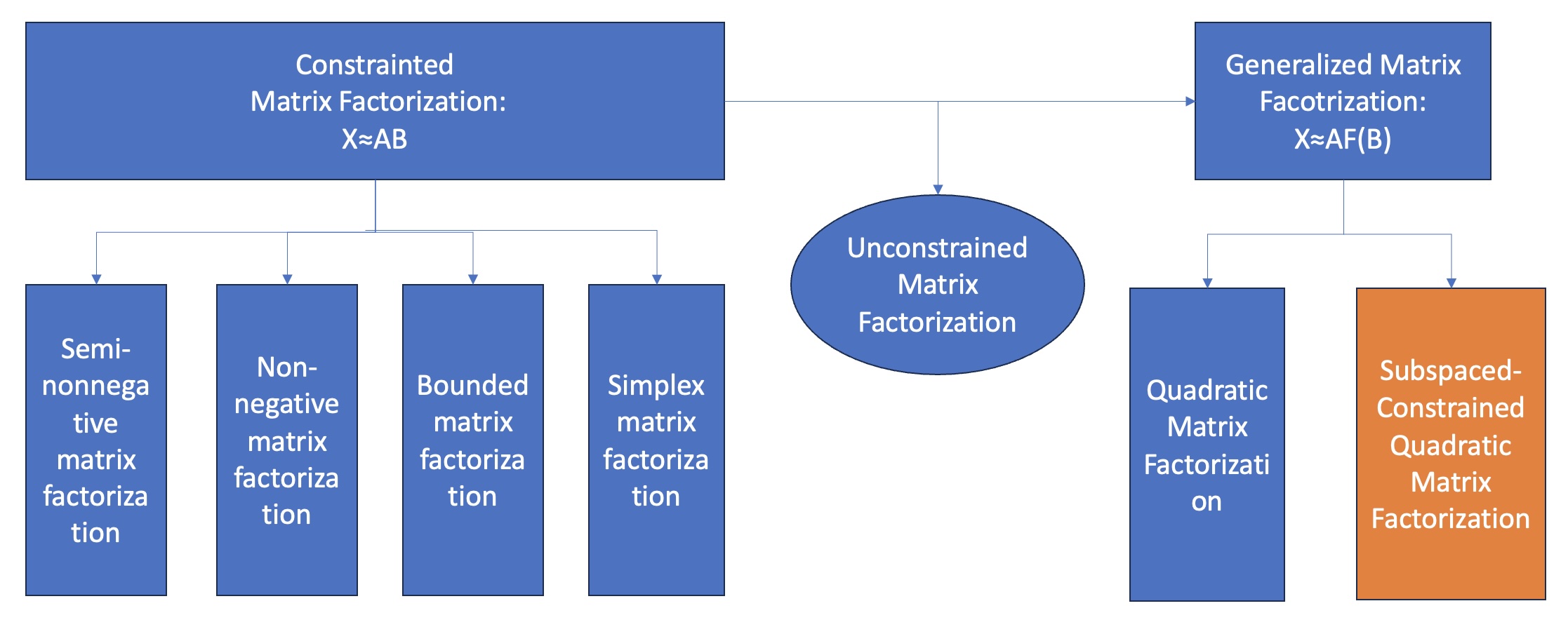
We categorize the global matrix factorization landscape into three distinct types: constrained matrix factorization, unconstrained matrix factorization, and generalized matrix factorization, as illustrated in Figure 1.
Unconstrained Matrix Factorization: The unconstrained factorization model, as presented in [37], seeks to optimize the following objective: . This model can be efficiently solved using Singular Value Decomposition (SVD) of , or through the eigenvalue decomposition of and . The absence of constraints provides greater flexibility, allowing the model to minimize factorization loss by freely adjusting both and .
Constrained Matrix Factorization: Introducing constraints on or limits the solution space, which typically leads to an increase in factorization loss due to the reduced flexibility. Various forms of constrained matrix factorization include nonnegative matrix factorization (NMF) [8], semi-nonnegative matrix factorization (Semi-NMF) [9], simplex matrix factorization (SMF) [10], bounded simplex matrix factorization (BSMF) [13] and manifold regularized matrix factorization (MMF) [11]. These models yield solutions tailored to different objectives: for instance, MMF produces a solution that preserves connectivity, while NMF generates one with improved clustering properties.
Generalized Matrix Factorization: Generalized matrix factorization extends beyond linear terms in by incorporating nonlinear functions , such as quadratic constructions. This advanced approach enhances the model’s ability to capture deeper, more intrinsic features within the data, resulting in a more accurate fit compared to traditional unconstrained models. An example of this is the quadratic matrix factorization model, as discussed in [28].
1.1.2 Manifold Fitting/Learning
Since we use our subspaced-constrained quadratic matrix factorization to learn the latent manifold, we also provide a concise overview of manifold fitting or denoising methods, encompassing various approaches such as local linear fitting (LPCA) [6], ridge-related techniques like KDE [14] and LOG-KDE [17], tangent space estimation through weighted summation (MFIT) [15], and higher-order regression methods like moving least squares (MLS) [16]. For the sake of comparison, we delve into seven methods in detail.
The most straightforward model for understanding the latent linear structure among datasets is local PCA (LPCA) [6] which fits the data with a model of where is the center and is orthonormal matrix. The estimator can be acquired through two steps: First, learning the center, such as , where are the samples in the local neighborhood. Second, computing the shifted covariance matrix . Let denote the projection matrix associated with the subspace spanned by the principal eigenvectors of . The denoised version of , representing a point on the estimated manifold projected from , is given by .
Apart from the local linear fitting methods, we can denoise or refine the data next to manifold by defining a subset that adheres to some conditions such as the ridge defined through kernel density estimation (KDE) [14] or logarithm kernel density estimation (LOG-KDE) [17]. Specifically, the ridge [14] is delineated via the Hessian and gradient of the density function as
| (6) |
where can be constructed nonparametrically. For example, , where is a kernel function with bandwidth . Additionally, , where the columns of are the leading eigenvectors of . The ridge (6) typically lacks closed-form solutions. In such cases, the subspace-constrained mean shift (SCMS) algorithm [17] is commonly employed to iteratively identify the ridge set. The LOG-KDE [17] ridge estimation method is essentially a kernel-based ridge estimation approach with substituted by . This modification impacts the covariance matrix and consequently results in a different estimation of the tangent space.
Similar to the ridge approach, alternative methods can be employed to define a smooth manifold under specific conditions related to the projection matrix. One notable method is manifold fitting (MFIT) [15], which constructs a manifold from noisy data using the following formulation: where represents a weight function, denotes the projection matrix related with the normal space at , and stands for the projection matrix corresponding to space spanned by the leading eigenvectors of . The function can be selected as , where is a normalized factor ensuring , represents the radius, and is the power parameter.
Additionally, we would like to discuss a relevant methodology for higher-order manifold estimation: the moving least squares method (MLS) [16]. This approach encompasses two key stages: identifying the appropriate tangent space and executing the regression step. Specifically, for any , it initially seeks the -dimensional hyperplane in that minimizes the following expression:
where is a weight function and is the distance between and . Subsequently, a coordinate system is established on with the origin being the projection point of onto . Utilizing this coordinate system, we can obtain the -dimensional representation of by projecting to . In the second step, a polynomial function of a specified degree is fitted by minimizing the following weighted squares: . The origin point of at is considered as the refined or denoised point of .
Spherical PCA (SPCA) [18] is a variant of LPCA which first learns a dimensional affine space parameterized by and projects the data into the affine space via . Then, the method learns a -dimensional sphere parameterized by the center and radius can be learned through:
After we obtain , for any data outside the sphere and , the projected point on the sphere can be achieved by: .
Structure-Adaptive Manifold Estimation (SAME) [19] is a diffusion method which aims to recover data from noisy observations using weighted averaging. The weights at are computed based on a suitable projector . Denote by the estimation of in the -th iteration. Then the update of at the -th iteration is given by
where weights are given by where is the -th bandwidth with a rate , is the initial bandwidth, and is a threshold. In SAME, is updated using the eigenvalue decomposition of the covariance matrix , where is an index set with .
Finally, it is also worth noting that the unconstrained regularized quadratic matrix factorization (RQMF) model has been explored in our prior research [28], wherein we propose a model represented as , with and . However, the proposed model in prior work diverges from the current model in two significant respects: Firstly, unlike the model proposed in [28], where and are treated as unconstrained parameters, we introduce explicit orthonormal restrictions on and . This imposition helps mitigate the correlation between the linear and quadratic terms, thereby enhancing the model’s fitting performance and mitigating the risk of over-fitting. Secondly, we reduce the number of free parameters by substituting the unconstrained tensor with an orthonormal matrix and an unconstrained tensor . This substitution notably diminishes the parameter search space, especially when is much smaller than , resulting in a more computationally efficient model. These modifications offer several advantages, including the development of more robust algorithms for optimizing the objective function.
1.2 Paper Organization
The rest of the paper proceeds as follows: In Section 2, we propose an alternating algorithm to solve the factorization model presented in (4). Specifically, we partition the factorization model into a regression sub-problem concerning and , and a projection sub-problem concerning . In Section 3, we study the convergence properties of the alternating minimization algorithm for solving the regression (inner iteration) and fitting model (outer iteration). In Section 4, we elaborate on three applications for the SQMF model. Subsequently, in Section 5, we present numerical simulations on both synthetic and real datasets, demonstrating the superiority of the SQMF over related methods.
1.3 Notation
| Symbol | Description |
|---|---|
| Three-order tensor which represents the second fundamental form, which is also an operator . | |
| Matrix with the shape of , which is the matrix form of . | |
| represents the basis for the tangent space and represents the basis for the normal space. . | |
| Shifting center for the coordinate system. | |
| The coordinate matrix whose -th column represents the coordinate for . | |
| Accumulation point of the sequences | |
| The quadratic coordinate matrix, whose -th column consists of the cross-product from the entries of . |
We present a concise overview of the frequently used notations in Table 1. The three-order tensor with the shape of is symmetric for its second and third dimensions, i.e., each of its slices is a symmetric matrix in . can also be seen as an operator from to such that the -th element of is . The matrix function maps the -th column of to the -th column of such as . The adjoint operator of , denoted as , is defined as , where represents the -th slice of . Let represent the action of on , defined as . We denote the operator norm and norm as and respectively. Additionally, denotes the -th largest singular value of matrix .
2 Subspace-Constrained Quadratic Matrix Factorization
In this section, we begin by establishing the loss bound for the RSQMF model. Following that, we introduce the algorithm for solving both SQMF and RSQMF models.
2.1 Solution Properties
Here, we study the relationship between three matrix factorization models: the unconstrained matrix factorization (MF), the subspace-constrained quadratic matrix factorization (SQMF) and the regularized subspace-constrained quadratic matrix factorization (RSQMF). For ease of notation, we introduce two sets: and .
Proposition 1.
Let , and be the optimal solution of RSQMF with extra constraint , the RSQMF model and the SQMF model, respectively. Then, we have:
Proof.
The first inequality is straightforward because is the optimal solution of SQMF. Next, we derive the second inequality. Recall that minimizes , and minimizes . Minimizing the same objective under the restriction of leads to an increase in the objective function:
which is equivalent to:
By eliminating the nonnegative item , we obtain the second inequality.
Notably, when the RSQMF model is restricted to , it simplifies to an unconstrained matrix factorization model. The proposition 1 indicates that although the regularized version of RSQMF increases the fitting error compared with SQMF, the error for RSQMF is still smaller than that of the unconstrained matrix factorization model, regardless of the choice of ().
2.2 Algorithm
This section explores the application of the alternating minimization algorithm to address SQMF in (4) and RSQMF in (5). As SQMF can be viewed as a special form of RSQMF with the tunable parameter , we just need to discuss the differences between SQMF and RSQMF when necessary.
To comprehensively tackle SQMF and RSQMF, we introduce two pivotal subproblems. The first subproblem is formulated by fixing at and optimizing the remaining parameters within or . Subsequently, the second subproblem is defined by fixing as and optimizing or with respect to . In other words, we iteratively solve the following two subproblems:
| (7) | ||||
If the sequence converges, we designate the convergence point as the solution to the joint minimization problem (4) and utilize the convergence point as the optimal solution. Since we also employ an alternating strategy to solve each of the subproblems in (7), we refer to the iteration in (7) as an outer iteration. Next, we will analyze and optimize both and in subsections 2.3 and 2.4 respectively. From the iterations in (7), it is evident that the function value decreases with the updating of the sequence , i.e.,
| (8) |
Recalling that for all , we can conclude that the sequence converges by the monotone convergence theorem. The decreasing relationship expressed in (8) further indicates that the model (4) improves in precision with each successive iteration step .
2.3 Alternating Method for Minimizing
In this subsection, we fix as and give an alternating approach to solve the first subproblem in (7). First, we can reformulate the problem using block multiplication, yielding:
| (9) |
Due to the block product relationship between and in (a) and the orthonormal constraint imposed on , a closed-form solution does not exist concerning . Nevertheless, an alternating perspective allows us to address this problem. In the following, we illustrate that the optimization problem with respect to any one of , when fixing the other two remaining parameters, admits a closed-form solution. For ease of notation, we denote and .
Note that the loss function includes an additional term , compared to . As a result, the main distinction in the alternating iterations lies in the updates for ; the optimal solutions related to and remain the same for both and when other parameters are fixed.
2.3.1 Optimize via Fixing
Here, we derive the closed-form solution of when and are held constant as and . By rearranging the objective function in (4), we can simplify the regression problem to optimize an orthonormal matrix that effectively aligns the columns of and . This alignment is achieved by minimizing the subsequent objective function:
| (10) |
Since is an orthonormal matrix with full column-rank, we have . Consequently, we can eliminate constants and transform the problem into an equivalent form:
| (11) |
Since any orthonormal matrix can be expressed as the product of two orthonormal matrices as with and , we can rewrite (11) as:
| (12) |
2.3.2 Optimize via Fixing
The problem in (4) with respect to is quadratic and thus convex, ensuring a global solution. By rearranging (4) to emphasize and fixing and as and , respectively, we can express (4) in the following equivalent form:
| (13) |
The above problem can be solved through its associated normal equation. Specifically, by computing the derivative with respect to , the solution to (13) can be obtained by solving the normal equation which leads to a closed-form solution .
2.3.3 Optimize via Fixing
For SQMF, the problem with respect to is also quadratic and we can derive the closed-form solution for through some projection manipulations. Since the spaces spanned by the columns of and are orthogonal, we can split the squared Frobenius norm of into:
| (14) |
Noticing that does not depend on , we can neglect this term and formulate (14) equivalently as
| (15) |
Since (15) is a regression problem, the optimizer of (15) can be found by solving the normal equation with respect to . Therefore, if has full row-rank, we have the explicit solution for as
| (16) |
For RSQMF, the procedure involving can be executed similarly to derive the closed-form solution for as follows:
| Input: and the coordinate matrix ; Dimensional parameters and , |
|---|
| which corresponds to the tangent space and subspace of the normal space, respectively. |
| Output: The center: ; The orthonormal matrix and which span the tangent space |
| and the subspace of the normal space, respectively; The quadratic curvature parameter . |
| (1). Set the initial value of as and as . |
| (2). While : |
| (3). Update: , with . |
| (4). Update: . |
| (5). Update: , with . |
| (6). Return . |
In summary, by updating each of and as in (11), (13) and (16) while fixing the remaining two parameters, we obtain a sequence of . If the sequence converges, we use the limit point as the solution for the regression problem. The stopping condition is defined as the total variation of , , and the spatial distance for the orthonormal matrix , with the maximum tolerance being . We present our iterative updating algorithm for the regression model in Table 2.
2.4 Optimize
In this subsection, we study how to optimize with respect to . Recall that the matrix-valued function is defined column-wise, and because the squared Frobenius norm is separable, solving reduces to solving a projection problem for each column of independently. Thus, we only need to optimize over each column variable, denoted here as , to achieve the desired result, by the following problem:
| (17) |
After solving (17) for , we can obtain by stacking each into a matrix, i.e., . Next, we further simplify (17) into the summation of two loss functions on the space of and . Since both of and are orthonormal matrices, we have:
| (18) | ||||
where and are the projection matrices corresponding to two orthogonal spaces. By defining and eliminating the term that is not relevant with , we can further simplify (18) into
| (19) |
In the following, we simplify notation by omitting the subscript and denoting as where context permits. For the regularized version, noting that is also a separable function, the problem with respect to each reduces to:
| (20) |
The optimization problems in (19) and (20) are nonlinear, presenting as quartic problems with respect to . Due to the high-order term involving , a closed-form solution is not feasible. Recognizing (19) as a specific case of (20) with , we focus on solving (20). We propose three approaches—Gradient Descent, Newton’s Method, and a Surrogate Method—to minimize (20). The theoretical properties of these methods are further analyzed in Section 2.7.
2.4.1 Gradient and Newton’s Methods
Gradient descent [32] is a commonly employed technique to minimize (20). Starting from an initial point , the gradient descent proceeds as follows:
where represents the step size. Practically, we set , with chosen as the smallest integer such that . While gradient descent can reach linear convergence rates, further acceleration can be achieved by incorporating Hessian information, as done in Newton’s method. Before presenting Newton’s method, we first derive the gradient and Hessian of as follows:
| (21) |
Newton’s method [34] can be understood as an approach that adjusts direction and step size using the inverse of the Hessian matrix. By utilizing the information in the Hessian, Newton’s method iteratively seeks the stationary point of through the following updates:
| (22) |
Unlike the gradient method, Newton’s method adaptively adjusts the step size through the Hessian matrix, removing the need for manual tuning. Instead of solving (20) directly with standard optimization methods, a surrogate approach can be developed by reducing the problem’s order, allowing for an iterative solution through the surrogate method, as discussed in the following sections.
2.4.2 Surrogate Method
Here, we propose an alternative approach that leverages surrogate functions to reduce the problem’s order by introducing an auxiliary function. Specifically, we lower the order of by incorporating an auxiliary function , defined as follows:
| (23) |
Due to the symmetry between and , the function in (23) satisfies . Thus, if is a minimizer of with , then also minimizes . In the sequel, we elaborate on how to find the minimizer of via the alternating minimization technique.
Starting from , we update iteratively in the following manner:
| (24) |
Through the iterations in (24), we generate a sequence of . Once this sequence converges, with , the limit point serves as the solution to the problem .
This surrogate method can be implemented efficiently as iterates in (24) admit closed-form solutions. Recall that yields a form as
| (25) |
Thus, minimizing (25) results in a quadratic function in terms of , allowing us to obtain the following closed-form solution:
| (26) |
Recognizing that is symmetric, minimizing with respect to can be addressed similarly as follows:
| (27) |
Till now, we have finished the algorithmic section for solving the subspace-contained quadratic matrix factorization model. In what follows, we will demonstrate that converges by showing that is a strongly convex function over and the sequence is contained in under certain conditions.
2.5 Comparisons of Optimization Strategies
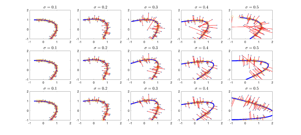
In this subsection, we examine the performance of three different approaches: Gradient, Newton, and the Surrogate method for solving the projection subproblem of (19). For the sake of a fair comparison, we employ the same alternating strategy to solve the regression problem in the outer iteration and compare the convergence behavior corresponding to the different strategies for the inner problem. The data is generated as , , where are sampled equally in , and .
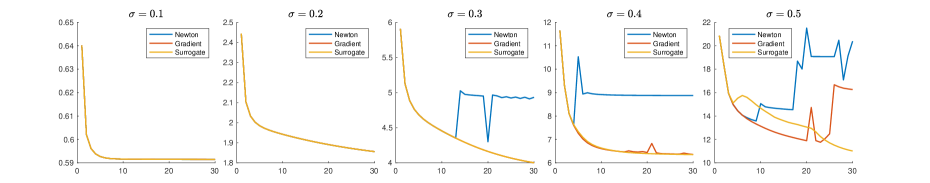
We illustrate the fitting result with the blue curve and also demonstrate how the noisy point is projected onto the fitted curve with a red line. Additionally, we plot how the fitting error, measured in the squared Frobenius norm , changes with the iteration steps in Figure 3. The total CPU time cost is reported in Table 3. From Figure 3 and Table 3, we can draw the following conclusions:
-
•
When the noise level is small, all three approaches exhibit a monotonically decreasing trend in the function value of the objective. However, as the noise level increases, this monotonically decreasing phenomenon no longer exists, as seen in in Figure 3.
-
•
Compared with Newton’s convergence curve, the gradient and surrogate methods demonstrate stronger robustness with the increasing value of . We observe that Newton’s method exhibits unstable convergence behavior for and , while the gradient and surrogate methods maintain stability.
The unsatisfactory convergence behavior of the three optimization methods is caused by the uncertainty regarding the convexity of for each as increases. Ensuring convergence behavior requires us to provide a theoretical justification for employing these methods to solve the projection problem (19) in the subsequent sections.
| Methods | |||||
|---|---|---|---|---|---|
| Newton | 0.04 | 0.04 | 0.07 | 0.04 | 0.04 |
| Gradient | 0.13 | 0.13 | 0.13 | 0.16 | 0.16 |
| Surrogate | 0.05 | 0.04 | 0.06 | 0.21 | 0.22 |
2.6 Complexity Analysis
In this section, we present a detailed analysis of the computational complexity of the RSQMF method. Given that RSQMF consists of two main components—regression and projection—we provide separate analyses for each step.
| Terms | ||||
|---|---|---|---|---|
| Complexity |
| Terms | |||
|---|---|---|---|
| Complexity |
The regression step involves updating the matrices , , and using equations (12), (13), and (16), respectively. This process includes the computation of , the Moore-Penrose inverse , and several matrix multiplications. Given that and has rows and columns, the computational complexity for updating is .
The construction of involves a matrix computation of , with a complexity of . Since and , the complexity for computing is . Therefore, the overall computational complexity for updating is .
For the computation of where , the complexity is . Additionally, updating requires performing a partial SVD corresponding to the previous eigenvectors, which costs for a matrix. Hence, the total computational complexity for updating is .
In the projection step, we solve equation (17) iteratively for each of the tasks. Each task is equivalent to solving problem (20) using either gradient, Newton, or surrogate methods. This requires computing the gradient , the inverse Hessian , and performing matrix multiplications, followed by executing steps like (22) or (26). In each projection step, the complexity for the gradient method is , while for the Newton and Surrogate methods, it is .
2.7 Theoretical Properties
In this section, we will elucidate the rationale for solving using Newton’s iteration and the surrogate method in (24), leveraging the strong convexity of within a local region of under certain conditions. The strong convexity can be verified by examining the Hessian of . For simplicity, we study the case for the non-regularized objective function by setting in .
Lemma 1.
Let and be the -th slice of for . If satisfies
| (28) |
then, for all . In other words, is strongly convex over the region .
The proof of Lemma 1 is postponed to the Appendix. We can draw two conclusions from observing (28): First, is strongly convex over as long as the maximum curvature, measured by , is not very large. Specifically, should be within the range . Second, for any , regardless of its magnitude, is strongly convex over as long as .
The strong convexity of , along with the symmetric property of , implies that there exists only one optimal solution as long as satisfies the condition in Lemma 1. This leads to our following theorem:
Theorem 1.
Suppose the conditions in Lemma 1 are satisfied and that generated by (24) resides within , then, converges as and . Furthermore, we have , where .
The proof of Theorem 1 is postponed to the Appendix. Theorem 1 requires that the sequence falls into , which is difficult to check. In what follows, we provide an upper bound for the sequence under mild conditions, such as .
Despite the absence of a closed-form solution for , valuable insights into the norm of the sequence can be gleaned from the iterations under certain mild conditions.
Proposition 2.
For any and , there exists such that the sequence , obtained from (24) satisfies for .
The proof of Proposition 2 is deferred to the Appendix. Based on Proposition 2, we can deduce that the upper bound for the norm at the convergence point is solely determined by and . In the limiting case where , the problem reduces to a linear projection, with as the projection of onto the tangent space, specifically = .
Corollary 1.
3 Convergence Properties
This section examines the convergence properties for both the inner and outer iterative updates. Specifically, we outline conditions under which the convergence point satisfies the Karush-Kuhn-Tucker (KKT) conditions [35] for the corresponding optimization problem. The results are presented here, with detailed proofs for Theorems 2 and 3 provided in the Appendix.
First, we analyze the convergence of the sequence when solving the regression problem (inner iteration) with fixed. We can conclude that any accumulation point will satisfy the KKT conditions, assuming the sequences have accumulation points and that is full row-rank.
Theorem 2.
If there exists a subsequence such that , and if the smallest eigenvalue of , then the sequence also converges, with . Furthermore, if the singular values of are distinct, the accumulation point satisfies the first-order Karush-Kuhn-Tucker (KKT) conditions for the problem in (4).
Second, we examine the convergence properties of the algorithm for the subspace-constrained quadratic matrix factorization problem (outer iteration). To facilitate this analysis, let us define the set , where is parameterized by , and is the tensor form of . We can then deduce that satisfies the Karush-Kuhn-Tucker (KKT) conditions of , where is any accumulation point of , and is uniquely determined by .
Theorem 3.
If there exists a sub-sequence such that and is a convex set depending on and . Then, also converges, and the accumulation point satisfies the Karush-Kuhn-Tucker (KKT) conditions of .
4 Applications
The subspace-constrained quadratic matrix factorization model fulfills two crucial roles: First, it assists in revealing the complex high-dimensional geometric structure inherent in a dataset. This encompasses tasks like refining noisy manifold-distributed data and inferring the tangent space at specific locations. Second, it facilitates the generation of a low-dimensional embedding representation within the latent space, which can be leveraged to elucidate the underlying patterns driving the variation trends in high-dimensional data.
4.1 Refining Noisy Manifold-Structured Data
The model RSQMF is adept at denoising manifold-structured data by learning a high-dimensional quadratic surface in a local region of . Through the formulation of a local quadratic fitting model in the vicinity , discrete data information is generalized into a continuous quadratic manifold. Afterwards, we can project onto the range of via a nonlinear least squares problem as . Therefore, we can measure the reconstruction error via the mean squared error over all the samples:
where and represent the projection of onto and the underlying truth for , respectively.
4.2 Tangent Space Estimation
The RSQMF model enables effective tangent space estimation. By fitting the data with RSQMF, we derive a representation , where the columns of define the tangent space at point . For an unknown point near , we estimate the tangent space at by locally adapting the tangent space defined by . This adaptive approach allows the model to capture variations in the tangent space within the local neighborhood of , enhancing the precision of tangent space estimation.
The reasoning behind this adjustment is as follows: by taking the derivative of with respect to , we find . Consequently, the tangent space at is shaped by altering the column space of with the column space of . Given that deviates from being an orthonormal matrix, we employ QR decomposition to yield , where is an orthonormal matrix and is an upper-triangle matrix. We then utilize the columns of as the basis for the adjusted tangent space at . In addressing a tangent space estimation problem for a set of points , we adopt the average distance between the estimated tangent space and the true underlying space as a criterion for evaluating the performance of the tangent estimator. Specifically, we define
where and represent the estimated and the underlying truth projection matrices for the tangent space at , respectively.
4.3 Enhanced Representation Capability
The SQMF or the RSQMF model exhibits enhanced representation capabilities, expressing data through the function . The linear term captures the principal signal, while the remaining part acts as a fine adjustment. The inclusion of the nonlinear term enables RSQMF to capture nonlinear signals, making it more versatile than traditional methods. In Section 5.3, we will demonstrate the superiority of RSQMF over related matrix factorization methods in reconstructing handwritten images with a latent representation in using the MNIST dataset. Additionally, the embeddings derived from RSQMF exhibit a more interpretable representation in the latent space compared to traditional matrix factorization methods.
5 Numerical Experiments
This section is structured into four key parts. First, we present a comparative analysis of RSQMF against five related algorithms, emphasizing its performance in manifold denoising (or fitting) and tangent space estimation. We also provide a detailed comparison of the computational costs associated with each method, measured in terms of CPU time. In the following part, we showcase the quadratic factorization model’s capability to capture variation trends in high-dimensional spaces by training RSQMF within a local neighborhood. Third, we apply RSQMF to a specially constructed two-class dataset, comprising randomly selected samples of the digits ‘4’ and ‘9’ from the MNIST dataset [29], demonstrating its superior image reconstruction abilities compared to other matrix factorization methods such as NMF [8], Semi-NMF [9], MMF [11], MF [37], and RQMF [28]. Lastly, we illustrate RSQMF’s effectiveness in denoising high-dimensional images, where it produces clean representations by utilizing information from neighboring data points. The code supporting this paper is available at https://github.com/zhaizheng/SQMF.
5.1 Experiments with Synthetic Data
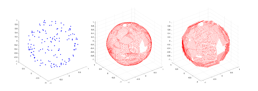
In this section, we perform a comparative analysis of RSQMF, MLS [16], LOG-KDE [17], MFIT [15], LPCA [6], and RQMF [28] using a synthetic spherical experiment. These methods are evaluated based on their ability to simultaneously denoise the manifold and estimate the tangent space, providing an assessment of their performance in both tasks. The data is generated through the following process: , where are uniformly distributed on a 2-dimensional sphere, and are i.i.d. Gaussian noise with , as depicted in the leftmost diagram in Figure 4. We employ the quadratic model proposed in our paper to learn the latent spherical manifold and its tangent space from the noisy dataset. It is worth mentioning that, in this specific case, the tangent space yields a rather simple estimator in the form of . This specific form of the tangent space allows us to conveniently evaluate recovery performance from both manifold and tangent space perspectives simultaneously. The recovery performance is illustrated in the middle and right diagrams in Figure 4.
| Methods | \ | 22 | 26 | 30 | 34 | 38 | 42 | 46 | 22 | 26 | 30 | 34 | 38 | 42 | 46 |
|---|---|---|---|---|---|---|---|---|---|---|---|---|---|---|---|
| RSQMF | 0.06 | 0.0007 | 0.0008 | 0.0008 | 0.0009 | 0.0010 | 0.0012 | 0.0014 | 0.0034 | 0.0037 | 0.0043 | 0.0052 | 0.0066 | 0.0079 | 0.0097 |
| 0.08 | 0.0013 | 0.0013 | 0.0014 | 0.0014 | 0.0016 | 0.0018 | 0.0020 | 0.0047 | 0.0047 | 0.0053 | 0.0059 | 0.0069 | 0.0074 | 0.0085 | |
| 0.10 | 0.0019 | 0.0019 | 0.0019 | 0.0020 | 0.0021 | 0.0022 | 0.0025 | 0.0072 | 0.0066 | 0.0072 | 0.0083 | 0.0100 | 0.0122 | 0.0138 | |
| MLS | 0.06 | 0.0008 | 0.0009 | 0.0010 | 0.0012 | 0.0015 | 0.0020 | 0.0026 | 0.0158 | 0.0168 | 0.0177 | 0.0173 | 0.0168 | 0.0166 | 0.0174 |
| 0.08 | 0.0013 | 0.0014 | 0.0015 | 0.0017 | 0.0020 | 0.0024 | 0.0029 | 0.0194 | 0.0220 | 0.0243 | 0.0244 | 0.0220 | 0.0212 | 0.0222 | |
| 0.10 | 0.0020 | 0.0020 | 0.0020 | 0.0021 | 0.0023 | 0.0026 | 0.0031 | 0.0252 | 0.0283 | 0.0267 | 0.0263 | 0.0221 | 0.0263 | 0.0266 | |
| LOG-KDE | 0.06 | 0.0161 | 0.0273 | 0.0485 | 0.0619 | 0.0933 | 0.0974 | 0.1197 | 2.6562 | 2.4458 | 2.2212 | 2.0194 | 1.8457 | 1.6962 | 1.5822 |
| 0.08 | 0.0171 | 0.0310 | 0.0455 | 0.0720 | 0.0971 | 0.1017 | 0.1005 | 2.8342 | 2.5540 | 2.1937 | 1.7409 | 1.4936 | 1.3412 | 1.2789 | |
| 0.10 | 0.0156 | 0.0296 | 0.0548 | 0.0908 | 0.1179 | 0.1548 | 0.1779 | 2.7181 | 2.4683 | 2.0651 | 1.7954 | 1.5867 | 1.4913 | 1.3757 | |
| MFIT | 0.06 | 0.0275 | 0.0495 | 0.0871 | 0.1747 | 0.2240 | 0.2429 | 0.2869 | 2.8358 | 2.7366 | 2.6293 | 2.4995 | 2.4235 | 2.2897 | 2.2252 |
| 0.08 | 0.0231 | 0.0337 | 0.0430 | 0.0509 | 0.0643 | 0.0899 | 0.0944 | 2.8854 | 2.8582 | 2.8236 | 2.7628 | 2.6508 | 2.4897 | 2.3754 | |
| 0.10 | 0.0246 | 0.0355 | 0.0484 | 0.0627 | 0.0847 | 0.1106 | 0.1353 | 2.8185 | 2.7353 | 2.6617 | 2.5680 | 2.4464 | 2.3008 | 2.1883 | |
| LPCA | 0.06 | 0.0113 | 0.0125 | 0.0154 | 0.0168 | 0.0190 | 0.0226 | 0.0296 | 1.9785 | 1.9762 | 1.9704 | 1.9675 | 1.9632 | 1.9560 | 1.9419 |
| 0.08 | 0.0102 | 0.0115 | 0.0129 | 0.0142 | 0.0130 | 0.0120 | 0.0139 | 1.9816 | 1.9790 | 1.9763 | 1.9736 | 1.9759 | 1.9780 | 1.9743 | |
| 0.10 | 0.0129 | 0.0163 | 0.0181 | 0.0215 | 0.0251 | 0.0301 | 0.0342 | 1.9778 | 1.9710 | 1.9676 | 1.9607 | 1.9533 | 1.9435 | 1.9353 | |
| RQMF | 0.06 | 0.0019 | 0.0029 | 0.0045 | 0.0064 | 0.0087 | 0.0117 | 0.0154 | 0.0269 | 0.0237 | 0.0229 | 0.0273 | 0.0296 | 0.0307 | 0.0292 |
| 0.08 | 0.0023 | 0.0033 | 0.0046 | 0.0065 | 0.0090 | 0.0121 | 0.0161 | 0.0284 | 0.0273 | 0.0286 | 0.0289 | 0.0253 | 0.0242 | 0.0243 | |
| 0.10 | 0.0031 | 0.0040 | 0.0053 | 0.0072 | 0.0097 | 0.0127 | 0.0164 | 0.0288 | 0.0295 | 0.0308 | 0.0298 | 0.0307 | 0.0302 | 0.0325 | |
| Methods | RSQMF | MLS | LOG-KDE | MFIT | LPCA | RQMF |
|---|---|---|---|---|---|---|
| Elapsed-Time | 1.977 | 0.017 | 1.942 | 2.804 | 0.009 | 1.094 |
To evaluate the performance of various methods under different noise levels and neighborhood sizes, we conducted experiments with noise levels set from and local region parameters defined as for . We set the regularization parameter for RSQMF. Similarly, we set for RQMF to mitigate the risk of overfitting. The evaluation metrics, and , are provided in Table 7, while the computational cost, measured in CPU time, is reported in Table 8.
Our findings indicate that RSQMF consistently outperforms the other five related methods, demonstrating superior accuracy with smaller fitting errors in both and . Notably, RSQMF exhibits heightened robustness in recovering the tangent space. This stands in contrast to LOG-KDE, MFIT and LPCA, which derive their latent representations through repeated implementations of the subspace constraint mean-shift algorithm. The convergence points reached by these methods may deviate significantly from the true projection, resulting in larger errors when estimating the tangent space. RSQMF outperforms RQMF due to its ability to independently handle and separate the tangent space from the normal space. This separation allows RSQMF to better capture local geometric structures, leading to improved performance in tasks such as manifold learning and tangent space estimation.
5.2 Image’s Variation in
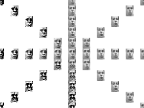
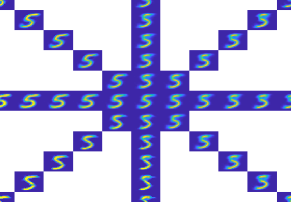
In this subsection, we study the models’ ability to capture the variation trend. We randomly select an image from the Frey Face dataset and utilize its 300 nearest neighbors in Euclidean space to train a quadratic factorization model with , , and . This function can be viewed as an image generator, decoding a low-dimensional vector in into an image in . Next, we manually construct in four directions: , , , and , by setting the local coordinate with in the range of . Finally, we display the images of at the positions of in Figure 5.
As we optimize an RSQMF model with a latent dimension , the task narrows down to interpreting the variation trends along each of the two dimensions. In the left panel of Figure 5, we observe two key patterns: First, moving from left to right along the horizontal axis reveals a gradual gender transition from a female face with glasses to a male face without glasses. Second, the direction of the vertical axis clearly influences facial expressions in the Frey Face dataset111Available at https://cs.nyu.edu/ roweis/data.html, with an increase in the vertical coordinate corresponding to a shift from a smiling expression to a more serious demeanor. In the right panel of Figure 5, we explore how the embedding coordinates in affect font style in the MNIST dataset [29]. As we move along the x-axis from lower to higher values, the horizontal stroke in the handwritten digit ‘5’ transitions from long to short. Additionally, the stroke style of ‘5’ evolves from sharp to smooth as we move along the vertical axis.
5.3 Latent Representation and Data Reconstruction
In this subsection, we tackle a more challenging task by applying RSQMF to learn a global model on a manually selected dataset. The complexity distribution of the chosen data adds to the challenge, primarily due to the potential existence of the indefinite second-order fundamental form matrices in .
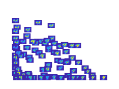
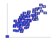
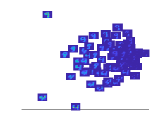
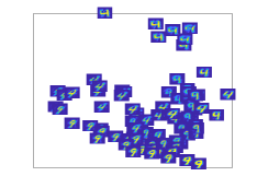
To provide further detail, we assemble an image set comprising two classes, each containing 150 randomly selected images representing ‘4’ and ‘9’ from the MNIST [29] dataset. We then proceed to train RSQMF with on this dataset. The resulting low-dimensional embeddings of are visualized in Figure 6, and the reconstructed images are depicted in Figure 7. We present the average fitting error measured by mean squared error and the clustering result of the embedding representation measured by accuracy (ACC) in Table 10. The elapsed CPU time for each method is also reported, with all methods evaluated under the same stopping criteria, defined as . For MMF, we set the trade-off parameter within the range and constructed the connection matrix using the Gaussian kernel. The results reported correspond to the configuration achieving the highest ACC. Finally, we investigate the parameter reliance and present the average fitting errors for the images corresponding to MF and RSQMF across different settings of and in Table 9.
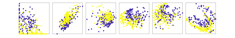
Upon examining Figure 6, it is evident that the embeddings for the digits ‘4’ and ‘9’ are distinctly separated by a curve, clearly delineating the two classes with a noticeable gap for RSQMF. In contrast, the embeddings generated by linear projection methods like NMF, Semi-NMF, MF, and RQMF exhibit significant overlap, making it more difficult to distinguish between the two classes. Furthermore, we illustrate the reconstructed images at their own embedding coordinates in Figure 7, where we can observe the variation trends with the two-dimensional coordinates. Finally, we compare the reconstruction capability for NMF, Semi-NMF, MMF, MF, RQMF and RSQMF in Figure 8.

| \ | 1 | 2 | 3 | 4 | 5 | 6 |
|---|---|---|---|---|---|---|
| 0.0 | 1.787(6.2%) | 1.700(10.1%) | 1.643(13.1%) | 1.606(15.1%) | 1.818(4.5%) | 1.773(6.6%) |
| 0.2 | 1.812(5.3%) | 1.727(9.8%) | 1.677(12.4%) | 1.643(14.1%) | 1.625(14.9%) | 1.713(9.4%) |
| 0.4 | 1.823(4.8%) | 1.751(8.8%) | 1.714(10.6%) | 1.672(12.9%) | 1.659(13.6%) | 1.650(14.1%) |
| 0.6 | 1.831(4.5%) | 1.768(8.0%) | 1.736(9.6%) | 1.698(11.6%) | 1.688(12.1%) | 1.677(12.8%) |
| 0.8 | 1.838(4.1%) | 1.783(7.2%) | 1.755(8.7%) | 1.720(10.5%) | 1.713(10.8%) | 1.701(11.6%) |
| Algorithms | NMF | Semi-NMF | MMF | MF | RQMF | RSQMF |
|---|---|---|---|---|---|---|
| MSE | 2.077 | 2.023 | 3.103 | 1.910 | 1.818 | 1.606 |
| ACC | 0.567 | 0.765 | 0.642 | 0.619 | 0.619 | 0.651 |
| Elapsed Time(s) | 0.13 | 0.21 | 0.84 | 0.10 | 4.75 | 1.11 |
To provide a more detailed comparison, we evaluate the performance of RSQMF by varying the parameter throughout the set and the normal space parameter over the range . After training RSQMF to obtain the reconstruction function , we compute the reconstruction error using the norm, defined as , where represents the reconstruction method, such as linear reconstruction by MF or orthonormal quadratic reconstruction via RSQMF. The fitting errors for RSQMF under various parameter settings are summarized in Table 9 for comparative analysis. From the observations in Figure 8, Table 9 and Table 10, we can conclude that:
-
1.
RSQMF consistently outperforms the optimal linear model of MF and other constrained MF methods, such as MMF, NMF and Semi-NMF, by achieving lower fitting errors across all parameter combinations. Additionally, as shown in Figure 8, RSQMF excels in capturing finer details compared to the competing methods, further highlighting its superior performance.
-
2.
The fitting performances across the six different methods are ranked as follows: , where stands for the mean squared error for NMF, with similar notations used for the other methods.
-
3.
When is small—specifically, when is less than 4 in this case—the performance of RSQMF tends to decline as increases. This degradation occurs because the stronger regularization term increasingly suppresses the influence of the quadratic component, leading to the model learning a flatter structure. As a result, the model’s ability to capture complex patterns diminishes, thereby reducing overall performance.
-
4.
As increases, for instance, when the normal space dimensional parameter takes values of 5 or 6 in this scenario, a properly selected can significantly enhance the performance of RSQMF.
We provide an explanation for the observed performance ranking in Table 10 as follows: Among fixed rank matrix factorization models, unconstrained matrix factorization (MF) achieves the lowest fitting error due to its flexibility. However, when nonnegativity constraints are introduced, the models become less flexible, leading to an increase in fitting error as a trade-off. Specifically, NMF incurs a higher fitting error than Semi-NMF because it imposes an additional constraint, further limiting the model’s adaptability. Manifold regularized matrix factorization (MMF) leads to relatively large fitting errors with suboptimal clustering performance. This is primarily due to the influence of the regularization term and the difficulty of constructing a reliable connection matrix in Euclidean space using an unsupervised approach, particularly for image data. In contrast, the quadratic factorization model leverages nonlinear fitting in the normal space, allowing it to capture more complex data patterns and thus outperform linear factorization models. Additionally, RSQMF surpasses RQMF due to its space-separation property and the reduced number of quadratic parameters, which contribute to enhanced stability and robustness. This combination of factors allows RSQMF to achieve superior performance in fitting tasks.
From both computational cost and clustering perspectives, as shown in Table 10, we observe the following: Matrix factorization (MF) incurs the lowest computational cost, as it only requires computing a partial SVD decomposition. Both NMF and Semi-NMF are relatively faster because they involve entrywise nonnegative updating, which are computationally efficient. In contrast, MMF is relatively slower because it requires computing the inverse of an matrix with each update. RQMF and RSQMF also incur higher computational costs, as they involve repeated regression and projection procedures. RSQMF demonstrates a relatively satisfactory performance in terms of ACC, though it does not perform as well as Semi-NMF.
Finally, we provide a rationale for introducing the regularization term when is large. The parameter represents the number of quadratic forms defined on the tangent space, and as increases, it becomes increasingly difficult to maintain the positive definite property of . This challenge leads to difficulties in ensuring the convergence of iterations for solving the projection problem, often resulting in unstable solutions. By introducing the regularization parameter , we can more easily satisfy the conditions necessary for to remain positive definite. Therefore, regularizing the model becomes essential when is relatively large to ensure stability and reliable convergence.
5.4 Image Refinement
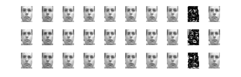
In this section, we provide a comprehensive analysis of RSQMF and seven other methods when applied to denoising blurred images. To simulate the noisy input, we introduce the white noise using , where each and represent images with dimensions , and is the noisy image. We assume each entry of follows a zero-mean uniform distribution, i.e., . We utilize the noisy images as input for eight denoising methods: RSQMF, MLS [16], LOG-KDE [17], MFIT [15], LPCA [6], SAME [19], SPCA [18] and RQMF [28], yielding corresponding outputs . A subset of 1000 images is randomly selected from , and their nearest neighbors are used to train an RSQMF model with . Finally, we project the noisy images back onto the quadratic function . We explore the neighborhood parameter with various sizes . The resulting images from different methods are displayed in Figure 9. The mean squared error, calculated as , is reported in Table 11. Spherelet under-performs because it heavily depends on an estimated radius, which can improperly compress or stretch the scale of the output. Notably, RSQMF with and outperforms the related methods, achieving a smaller fitting error. This observation is coherent with our intuition that the curvature information can help us better capture the nonlinear distribution contained in the data.
| \ Alg | RSQMF | MLS | LOG-KDE | MFIT | LPCA | SAME | SPCA | RQMF |
|---|---|---|---|---|---|---|---|---|
| 16 | 1.632 | 2.475 | 2.043 | 2.561 | 2.022 | 2.112 | 342.339 | 1.771 |
| 20 | 1.627 | 2.025 | 2.097 | 2.581 | 2.106 | 2.148 | 344.413 | 1.707 |
| 24 | 1.652 | 2.027 | 2.301 | 2.669 | 2.111 | 2.203 | 345.367 | 1.781 |
| 28 | 1.666 | 1.989 | 2.358 | 2.902 | 2.137 | 2.210 | 344.338 | 1.717 |
| 32 | 1.743 | 2.044 | 2.403 | 2.894 | 2.152 | 2.276 | 339.628 | 1.786 |
6 Conclusion
This paper introduces a subspace-constrained matrix factorization model, along with algorithms and theoretical insights regarding the solving process and convergence behavior. The strengths of our model can be highlighted as follows: First, the model captures nonlinear structures within the data, allowing for the extraction of richer feature details compared to linear models. Second, unlike previous quadratic matrix factorization approaches, we incorporate an additional subspace constraint that helps decouple the mutual influence between the tangent and normal spaces, improving the model’s precision. Third, by reducing the number of quadratic parameters to be optimized, our model demonstrates greater stability and is less prone to overfitting. Lastly, the curvature variables in our regularized quadratic model can be flexibly adjusted using the parameter , making the model highly adaptable to various tasks.
However, there are also some shortcomings and unexplored areas that warrant further investigation. First, while incorporating the quadratic form within a subspace is beneficial, we have not explored how to optimally select the dimension parameter . Our experiments indicate that significantly affects the performance, and further research is needed to understand its optimal selection. Second, although the model shows strong performance across tasks, its computational process involves both outer updates for the regression and projection problem, as well as inner updates for parameters during the regression step. Due to space and time constraints, we did not delve into speed-up strategies, an area that could improve the efficiency of our approach in future work.
Several promising directions for future research emerge. First, beyond quadratic terms, more intricate structures, such as higher-order polynomials or other nonlinear functions, could be explored to better capture the underlying data distribution. Second, while our method focuses on unsupervised learning, applying it to supervised tasks, like predicting data labels, presents an exciting new direction. Third, the statistical properties of the SQMF model, such as those from a non-asymptotic perspective, offer potential avenues for future exploration. Given the manifold’s complexity, there are still several unexplored aspects that could lead to novel applications and deeper insights, which we plan to investigate in future research.
Acknowledgment
This work was supported by the National Natural Science Foundation Funds under Grants of 11801592 and 12301478.
References
- [1] Jialu Liu, Chi Wang, Jing Gao, and Jiawei Han. Multi-view clustering via joint nonnegative matrix factorization. In Proceedings of the 2013 SIAM international conference on data mining, pages 252–260. SIAM, 2013.
- [2] Yehuda Koren, Robert Bell, and Chris Volinsky. Matrix factorization techniques for recommender systems. Computer, 42(8):30–37, 2009.
- [3] Qi Wang, Xiang He, Xu Jiang, and Xuelong Li. Robust bi-stochastic graph regularized matrix factorization for data clustering. IEEE Transactions on Pattern Analysis and Machine Intelligence, 44(1):390–403, 2022.
- [4] Pentti Paatero and Unto Tapper. Positive matrix factorization: A non-negative factor model with optimal utilization of error estimates of data values. Environmetrics, 5(2):111–126, 1994.
- [5] William L Hamilton, Rex Ying, and Jure Leskovec. Representation learning on graphs: Methods and applications. arXiv preprint arXiv:1709.05584, 2017.
- [6] Nanda Kambhatla and Todd Leen. Dimension reduction by local principal component analysis. Neural Computation, 9:1493–1516, 10, 1997.
- [7] Wang, Y.X. and Zhang, Y.J.. Nonnegative matrix factorization: A comprehensive review. IEEE Transactions on knowledge and data engineering, 25(6), pp.1336-1353, 2012.
- [8] Nicolas Gillis. Nonnegative matrix factorization. Society for Industrial and Applied Mathematics, 2020.
- [9] Nicolas Gillis, and Abhishek Kumar. Exact and heuristic algorithms for semi-nonnegative matrix factorization. SIAM Journal on Matrix Analysis and Applications, 1404-1424, 2015.
- [10] Abdolali, M., Gillis, N.. Simplex-structured matrix factorization: Sparsity-based identifiability and provably correct algorithms. SIAM Journal on Mathematics of Data Science, 593-623, 2021.
- [11] Zhang, Zhenyue, and Keke Zhao. Low-rank matrix approximation with manifold regularization. IEEE transactions on pattern analysis and machine intelligence 35.7: 1717-1729, 2012.
- [12] Singh, Ajit P., and Geoffrey J. Gordon. A unified view of matrix factorization models. Joint European Conference on Machine Learning and Knowledge Discovery in Databases. Berlin, Heidelberg: Springer Berlin Heidelberg, 2008.
- [13] Thanh, Olivier Vu, Nicolas Gillis, and Fabian Lecron. Bounded simplex-structured matrix factorization: Algorithms, identifiability and applications. IEEE Transactions on Signal Processing 71: 2434-2447, 2023.
- [14] Christopher R Genovese, Marco Perone-Pacifico, Isabella Verdinelli, Larry Wasserman, et al. Nonparametric ridge estimation. The Annals of Statistics, 42(4):15111545, 2014.
- [15] Charles Fefferman, Sergei Ivanov, Yaroslav Kurylev, Matti Lassas, and Hariharan Narayanan. Fitting a putative manifold to noisy data. In Conference On Learning Theory, pages 688–720, 2018.
- [16] Barak Sober and David Levin. Manifold approximation by moving least-squares projection (mmls). Constructive Approximation, 52(3):433–478, 2020.
- [17] Umut Ozertem and Deniz Erdogmus. Locally defined principal curves and surfaces. Journal of Machine learning research, 12(Apr):1249–1286, 2011.
- [18] Didong Li, Minerva Mukhopadhyay, and David B. Dunson. Efficient Manifold Approximation with Spherelets. Journal of the Royal Statistical Society Series B:Statistical Methodology, 84(4):1129–1149, 04 2022.
- [19] Nikita Puchkin and Vladimir Spokoiny. Structure-adaptive manifold estimation. Journal of Machine Learning Research, 23(1):1886–1947, 2022.
- [20] Aamari, Eddie, and Clement Levrard. Nonasymptotic rates for manifold, tangent space and curvature estimation. Annals of Statistics, 177-204. 2019.
- [21] Kaslovsky DN, Meyer FG. Non-asymptotic analysis of tangent space perturbation. Information and Inference: a Journal of the IMA. 3(2):134-187, 2014.
- [22] Kendall E. Atkinson. An Introduction to Numerical Analysis. John Wiley & Sons, Inc, ISBN 0471624896, 1989.
- [23] Wall, M.E., Rechtsteiner, A. and Rocha, L.M.. Singular value decomposition and principal component analysis. In A practical approach to microarray data analysis, pp.91-109, 2003.
- [24] Vincent Divol. Measure estimation on manifolds: an optimal transport approach. Probability Theory and Related Fields, 183(1):581-647, 2022.
- [25] Eddie Aamari. Clément Levrard. Nonasymptotic rates for manifold, tangent space and curvature estimation. Ann. Statist. 47 (1):177-204, 2019.
- [26] Golub, G.H. and Reinsch, C.. Singular value decomposition and least squares solutions. In Handbook for Automatic Computation: Volume II: Linear Algebra, pp.134-151, 1971.
- [27] Aizenbud, Yariv and Barak Sober. Non-Parametric Estimation of Manifolds from Noisy Data. arXiv preprint arXiv:2105.04754, 2021.
- [28] Zheng Zhai, Hengchao Chen and Qiang Sun, Quadratic Matrix Factorization with Applications to Manifold Learning, IEEE Transactions on Pattern Analysis and Machine Intelligence, 46(9):6384-6401, 2024.
- [29] Deng, L.. The mnist database of handwritten digit images for machine learning research. IEEE Signal Processing Magazine, 29(6):141–142, 2012.
- [30] Rapcsák, Tamás. On minimization on Stiefel manifolds. European Journal of Operational Research, 143(2): 365-376, 2002.
- [31] Fan, Yuling, Jinghua Liu, Peizhong Liu, Yongzhao Du, Weiyao Lan, and Shunxiang Wu. Manifold learning with structured subspace for multi-label feature selection. Pattern Recognition, 120(Dec), 2021.
- [32] Zhou, B., Gao, L. and Dai, Y.H.. Gradient methods with adaptive step-sizes. Computational optimization and applications, 35, pp.69-86, 2006.
- [33] Feng, W., Wang, Z., Cao, X., Cai, B., Guo, W. and Ding, W.. Discriminative sparse subspace learning with manifold regularization. Expert Systems with Applications, 249, p.123831, 2024.
- [34] Polyak, B.T.. Newton’s method and its use in optimization. European Journal of Operational Research, 181(3): pp.1086-1096, 2007.
- [35] Boyd, S.P. and Vandenberghe, L.. Convex optimization. Cambridge university press, 2004.
- [36] Zhang, Z. and Zha, H.. Principal manifolds and nonlinear dimensionality reduction via tangent space alignment. SIAM journal on scientific computing, 26(1): pp.313-338, 2004.
- [37] Singh, Ajit P., and Geoffrey J. Gordon. A unified view of matrix factorization models. Joint European Conference on Machine Learning and Knowledge Discovery in Databases, 2008.