A Structured Estimator for large Covariance Matrices in the Presence of Pairwise and Spatial Covariates

Abstract

We consider the problem of estimating a high-dimensional covariance matrix from a small number of observations when covariates on pairs of variables are available and the variables can have spatial structure. This is motivated by the problem arising in demography of estimating the covariance matrix of the total fertility rate (TFR) of $195$ different countries when only $11$ observations are available. We construct an estimator for high-dimensional covariance matrices by exploiting information about pairwise covariates, such as whether pairs of variables belong to the same cluster, or spatial structure of the variables, and interactions between the covariates. We reformulate the problem in terms of a mixed effects model. This requires the estimation of only a small number of parameters, which are easy to interpret and which can be selected using standard procedures. The estimator is consistent under general conditions, and asymptotically normal. It works if the mean and variance structure of the data is already specified or if some of the data are missing. We assess its performance under our model assumptions, as well as under model misspecification, using simulations. We find that it outperforms several popular alternatives. We apply it to the TFR dataset and draw some conclusions.

, , , , , and

1 Introduction

We consider the problem of estimating a large covariance matrix from a small number of data points when covariates on pairs of variables and their spatial structure are available. This is motivated by the problem, arising in demographic research, of estimating the covariance matrix of the total fertility rate for a large number of countries from data at a small number of time points.

Our specific goal is to estimate the covariance matrix of a model for the total fertility rate (TFR) used by the United Nations (UN) for 195 different countries. The dataset is denoted $Y$ and is made up of measurements of the TFR at $T=11$ time points (observations) for $d=195$ countries (variables). Each time point is a five-year period. The large dimension of the covariance matrix makes the use of a standard estimator, such as the sample covariance matrix, untenable, and necessitates the use of additional information. Fortunately, for the TFR dataset, we have been able to obtain information about pairwise, time-invariant, covariate structures. In particular, these include a spatial structure (e.g., countries being contiguous to each other), and structures determined by cluster membership (e.g., countries belonging to the same region, countries having the same common colonizer). The framework we propose also allows us to include interactions when modeling a covariance matrix.

Covariance matrix estimation

As we shall see, the performance of standard covariance matrix estimators is not excellent in the setting we consider, because they cannot handle pairwise and spatial covariates. These include shrinkage estimators, such as the Ledoit-Wolf estimator (Ledoit and Wolf, 2004), which shrink covariance matrices towards sparse matrices or the identity matrix (for a review, see Pourahmadi, 2013; Ledoit and Wolf, 2022), as well as estimators such as the graphical lasso (Friedman et al., 2008), which assumes sparsity of the inverse of the covariance matrix.

The most commonly used approaches which assume dependency structures within the model are approaches that use factor models (for an overview of these approaches, see Fan et al., 2016). There are indeed estimation procedures that use factor models and which can also allow for the encoding of spatial information, as in Christensen and Amemiya (2003); Wang and Wall (2003); Gamerman et al. (2008); Lopes et al. (2011); Thorson et al. (2015). Clustered structures, on the other hand, are estimated via multilevel factor models (Longford and Muthén, 1992). While we will show that the correlation structures of the different cluster effects present in the data can each be interpreted in the framework of multilevel factor models, none of the models available in the literature can combine several multilevel factor models with a spatial structure. Moreover, the number of samples we are facing is too small to use techniques such as parallel factor analysis (Harshman and Lundy, 1994).

Interpretability

Interpretability of the model parameters has been stressed to be an important feature of covariance matrix parametrization by Pourahmadi (1999, 2011), but while that work does provide solutions, they do not incorporate pair-specific covariates into the covariance matrix estimation procedure. Approaches that do include pairwise covariates into the model have involved evaluating linear combinations of known matrices on the scale of the covariance matrix (Anderson, 1973). Sums of covariance matrices also appear in linear mixed-effect models when adding crossed effects (Gałecki and Burzykowski, 2013).

However, sums of covariance matrices are, in practice, hard to interpret. To illustrate this problem, suppose that we set the covariance matrix of the data to the sum of the following two covariance matrices:

$$\Sigma:=\begin{pmatrix}18&0\\ 0&18\end{pmatrix}+\begin{pmatrix}2&0.8\\ 0.8&2\end{pmatrix},$$ (1)

and that a two dimensional Gaussian model with covariance matrix $\Sigma$ is used to model the data. The first matrix assumes independence between the two variables considered, while the second matrix characterizes variables which are clearly correlated. Individually, the correlations of the second matrix tell us nothing about the correlation matrix of the data, since they might be overwhelmed by the entries of the first. Indeed, while the correlations of the two variables associated with the second matrix are relatively high (0.4), the correlation matrix associated with $\Sigma$ is given by

$$R=\begin{pmatrix}1&0.04\\ 0.04&1\end{pmatrix},$$ (2)

meaning that the correlation between the two variables is small in the resulting dataset.

Different scales, such as the matrix logarithm (Chiu et al., 1996), have been suggested, but they suffer from a similar problem. Bonat and Jørgensen (2016) generalized these approaches into a framework for non-normal multivariate data, called multivariate covariance generalized linear models (McGLM). A McGLM was used by Bonat and Jørgensen (2016) to include spatio-temporal covariates in the covariance estimation. It is also possible to use Cavazani de Freitas et al. (2022) to incorporate information about variables belonging to a similar cluster. However, while the framework of McGLM is the closest to ours, it is not clear how to use it to get interpretable results, or how to combine spatial structures and clusters in the same model.

Some Bayesian approaches get interpretable parameters by separating the structure of the variance parameters from the structure of the correlation parameters. This separation strategy has been used successfully in Bayesian inference, in a variety of approaches (see for instance Barnard et al., 2000; Lewandowski et al., 2009; Tokuda et al., 2011). There are also some Bayesian approaches for covariance matrix estimation which use information about different clusters of variables, such as Karolyi (1992, 1993); Aguilar and West (2000); Bernardo et al. (2003); Liechty et al. (2004), but none of these combine this information with a spatial structure.

At the core of the covariance matrix estimation strategy we propose is the idea of combining the separation strategy with the approach of Anderson (1973). This allows us to normalize the covariance matrices into correlation matrices, such that the parameters of the random effects are interpretable. Going back to Equations (1) and (2), we recommend instead separating the variance estimation and modeling $R$ directly as a convex combination of two correlation matrices. In our previous toy example, a possible choice could be:

$$R=0.9\begin{pmatrix}1&0\\ 0&1\end{pmatrix}+0.1\begin{pmatrix}1&0.4\\ 0.4&1\end{pmatrix}.$$

The importance of each matrix is given by its linear coefficient. Independently of the values of the other matrix, we will know that the correlation between the two variables is such that 10 percent of the correlation structure is explained by the second correlation matrix.

In the TFR dataset that motivates our work, a variety of effects and their interactions are to be taken into account. We will show that the setting of the TFR dataset allows us to give useful estimates that work well, in the sense that useful properties (identifiability, consistency, asymptotic normality in the number of data points $T$ and in the dimension $d$, available confidence regions) hold under some assumptions. We will also adjust our estimator in such a way that it gives consistent estimates, without having to assume that specific model assumptions hold.

Outline of the paper

The manuscript is organized as follows. In Section 2, we give an overview of the dataset and give the motivation for our model assumptions, followed by the general setting for the estimator we propose. In Section 3, we define our estimator and derive its properties. We show how to estimate the parameters of our estimator (Section 3.3) and how to adjust it in the case that the model assumptions do not hold (Section 3.4). In Section 4 we assess its performance under a variety of different settings by simulation, and compare it to some popular alternative methods. Then, we use these techniques to derive estimates of the covariance matrix of the TFR dataset, whose correlations we compare in Section 5. We close with a discussion of our work. The code for this paper is made available via Github for scientific dissemination, see the following link.

2 Modelling covariance matrices with known pairwise and spatial covariates

2.1 The total fertility rate data

The dataset we analyze consists of the total fertilty rate (TFR) of 195 countries in successive $5$-year periods from 1950 to 2010. One country as well as one time period were removed for reasons on which we will elaborate further in this section and Section 5. The dataset is denoted by $Y$ and is made up of $T=11$ time points (observations) and $d=195$ countries (variables). The element $Y_{t,j}$ of $Y$ is the TFR of country $j$ at time $t$, and $Y_{t}^{\intercal}:=(Y_{t,1},\dots,Y_{t,d})\in\mathbb{R}^{d}$ denotes row $t$ of matrix $Y$. Note that the index $t$ is used to refer to different observations because of the specific nature of the dataset. There is previous work on this dataset, on which we build. We will first summarize this work.

Fosdick and Raftery (2014) found that the model then used by the United Nations (UN) to predict the total fertility rate (TFR) of different countries yielded prediction intervals for forecasting regions consisting of multiple countries that were too narrow. They found that this was due to between-country dependencies that are not included in the Bayesian hierarchical model of Alkema et al. (2011a), which was used for these predictions. To tackle this, Fosdick and Raftery proposed estimating the covariance matrix of the joint distribution of the countries’ TFRs.

They did this by modeling the covariance matrix using time-invariant pairwise information, namely whether two countries had the same common colonizer after 1945, whether two countries are contiguous, and whether two countries are in the same UN region.

A first model was built as

$$Y_{t} = \mu_{t}+\varepsilon^{0}_{t},\quad\varepsilon^{0}_{t}\sim\text{MVN}_{d}(0_{d},\Sigma_{t}),$$

with independent forecast errors $\varepsilon_{t}^{0}$, $\mu_{t}^{\intercal}:=(\mu_{t,1},\dots,\mu_{t,d})$, where $\mu_{t,j}$ denotes the expected TFR (conditional on $Y_{t-1}$) for country $j$ in period $t$ for $j\in\llbracket 1,d=195\rrbracket$ and $\Sigma_{t}$ the covariance matrix (conditional on $Y_{t-1}$), $t\in\llbracket 1,T=11\rrbracket$. Fosdick and Raftery (2014) also decomposed the covariance structure of the model into the standard deviation vector at time $t$, $\sigma_{t}\in\mathbb{R}^{d}_{+}$, as well as a correlation structure $R_{t}$. Conditional on $Y_{t-1}$, we have that:

$$\varepsilon^{0}_{t}\sim\text{MVN}_{d}(0_{d},\text{diag}(\sigma_{t})R_{t}\text{diag}(\sigma_{t})),$$

where $\text{diag}(\sigma_{t})$ is a diagonal matrix with entries $\sigma_{t}$ and $\textrm{MVN}_{d}(m,S)$ denotes the multivariate normal distribution of dimension $d$ with mean $m$ and covariance matrix $S$.

With the method of Alkema et al. (2011a) already providing accurate estimates of $\mu_{t}$ and $\sigma_{t}$, Fosdick and Raftery chose to model $\varepsilon_{t}$, the standardized version of $\varepsilon^{0}_{t}$, such that

$$\varepsilon_{t}\sim\text{MVN}_{d}(0_{d},R_{t}),$$ (3)

and focused on the estimation of $R_{t}$. For all countries that are in phase II or III of the model of Alkema et al. (2011a), they set

$$(R_{t})_{i,j}=\begin{cases}1\textrm{ if }i=j,\\ \alpha^{(1)}_{0}+\alpha^{(1)}_{1}\mathrm{contig}_{i,j}+\alpha^{(1)}_{2}\mathrm{comcol}_{i,j}+\alpha^{(1)}_{3}\mathrm{region}_{i,j}\text{ if }\;Y_{t,i}<\kappa\textrm{ and }Y_{t,j}<\kappa,\\ \alpha^{(2)}_{0}+\alpha^{(2)}_{1}\mathrm{contig}_{i,j}+\alpha^{(2)}_{2}\mathrm{comcol}_{i,j}+\alpha^{(2)}_{3}\mathrm{region}_{i,j}\textrm{ otherwise,}\end{cases}$$ (4)

where $\kappa$ is a threshold parameter, $\mathrm{contig}_{i,j}=1$ if countries $i$ and $j$ are contiguous, $\mathrm{comcol}_{i,j}=1$ if they had a common colonizer after 1945, $\mathrm{region}_{i,j}=1$ if they are in the same UN region, and $0$ otherwise.

The problem with this approach is that the value of $R_{t}$ that it yields is not necessarily positive definite for all values of $\alpha_{0}^{(k)},\dots,\alpha_{3}^{(k)}$. To address this, Fosdick and Raftery (2014) mapped their estimate of $R_{t}$ onto the positive definite correlation matrix that was closest to it with regards to the Frobenius norm. This is quite simply done computationally, by taking the eigenvalue decomposition of the estimated matrix, setting negative eigenvalues to a small positive value, and reconstituting the matrix. However, this method comes with no statistical guarantees. We seek instead a statistically principled approach to estimating the covariance matrix.

Here we propose a new approach that models the correlation matrix of the TFR directly, as a time-independent correlation matrix $R$, which is a linear combination of several correlation matrices. These correlation matrices are in turn entirely determined by known covariates, independent of the thresholding level $\kappa$, and in particular of the time point $t$, which is why we do not use the index $t$ for $R$ in our model. Therefore, $R$ will be positive definite if at least one of these correlation matrices is positive definite.

For each time point $t$, we follow Fosdick and Raftery (2014) in only modeling the TFR $Y_{t}$ of the countries that are in phase II or III of the model of Alkema et al. (2011a). This occurs only after the first time period, which is why one time period was removed to obtain $T=11$. Our methodology relies on the decomposition of the stanadardized errors $\varepsilon_{t}$ as a weighted sum of standardized, independent effects. Thus, for every time point $1\leq t\leq T$, we consider:

$$Y_{t} = \mu_{t}+\text{diag}(\sigma_{t})\varepsilon_{t},\quad\varepsilon_{t}\sim\text{MVN}_{d}(0_{d},R).$$

We model the residuals as follows:

$$\varepsilon_{t} = A_{t}+B_{t}+C_{t}+D_{t}+E_{t},\textrm{ }A_{t},B_{t},C_{t},D_{t},E_{t}\in\mathbb{R}^{d}\textrm{ where}$$ (5)

$$A_{t} \stackrel{{\scriptstyle\text{i.i.d}}}{{\sim}} {\rm MVN}_{d}(0_{d},\alpha_{A}F_{A}),\quad B_{t}\stackrel{{\scriptstyle\text{i.i.d}}}{{\sim}}{\rm MVN}_{d}(0_{d},\alpha_{B}F_{B}),\quad C_{t}\stackrel{{\scriptstyle\text{i.i.d}}}{{\sim}}{\rm MVN}_{d}(0_{d},\alpha_{C}F_{C}),$$

$$D_{t} \stackrel{{\scriptstyle\text{i.i.d}}}{{\sim}} {\rm MVN}_{d}(0_{d},\delta_{D}\Gamma(\beta_{D})^{-1}),\quad E_{t}\stackrel{{\scriptstyle\text{i.i.d}}}{{\sim}}{\rm MVN}_{d}(0_{d},\alpha_{E}I_{d}).$$

Note that the covariance matrix of the standardized errors is equal to the correlation matrix of the data, conditional on the values at the previous time points, since by construction each $\varepsilon_{t,j}$ has variance 1.

The random vectors, $A_{t,j},B_{t,j},C_{t,j},D_{t,j}$ denote the random effects on country $j$ at time $t$, corresponding to the effect of having a common colonizer, belonging to the same region, the global effect, the contiguity effect, respectively. The random vector $E_{t}$ denotes i.i.d Gaussian noise for all countries at time $t$ (its correlation matrix is the identity matrix of dimension $d$, $I_{d}$). Its presence ensures that the correlation matrix of $\varepsilon_{t}$ is positive definite, since at least one of the correlation matrices of the standardized effects is positive definite. The random effects are standardized, in the sense that the matrices $F_{A},F_{B},F_{C},\Gamma(\beta_{D})^{-1}$ are correlation matrices, i.e., positive semidefinite matrices with diagonal entries equal to 1. They are also weighted by positive constants $\alpha_{A},\dots,\alpha_{E},\delta_{D}$, which must sum to one. This ensures that the impact of each effect is measurable via its linear coefficient: for every pair of countries $(i,j)$, its correlation is an average of the individual entries $(F_{A})_{i,j},(F_{B})_{i,j},(F_{C})_{i,j},\Gamma(\beta_{D})^{-1}_{i,j}$ weighted by their respective weights.

We use two separate approaches for modeling the correlation matrices of the random effects. Matrices with the capital letter $F$ naturally impose a block structure on the model, in the sense that they partition the countries based on which cluster (i.e., region, colonizer) they belong to. Let $f_{A}\in\{0,1\}^{d\times 10},f_{B}\in\{0,1\}^{d\times 21}$ denote the covariates corresponding to the regional and common colonizer clusters, meaning that $(f_{B})_{j,r}=1$ if country $j$ belongs to region $r$ and $0$ otherwise (analogously for $f_{A}$). We can easily transform these covariates into correlation matrices by setting $F_{A}=f_{A}f_{A}^{\intercal},F_{B}=f_{B}f_{B}^{\intercal}$, meaning that $(F_{A})_{i,j},(F_{B})_{i,j}$ are equal to 1 if countries $i$ and $j$ have the same common colonizer or belong to the same UN region, respectively. The global effect applies equally to every country pair, such that $F_{C}=1_{d}1_{d}^{\intercal}$, where $(1_{d})_{j}=1$ for all $j$, meaning that $(F_{C})_{i,j}$ is always 1. Note that the way these matrices are modeled corresponds to the way in which correlation matrices are modeled in multilevel factor models, only that in our case the factor loadings and group means are known. They can also be represented via the design matrix of a linear mixed-effects model. We elaborate on these points in Appendix D.

The contiguity effect was modeled using a conditional autoregressive (CAR) model. There are many different CAR models, each of which is usually specified by a small number of parameters (Wall, 2004; Kyung and Ghosh, 2010; MacNab, 2011; Tastu et al., 2013; Ver Hoef et al., 2018). We parametrize the CAR model via only one autocorrelation parameter, $\beta_{D}$, in a Gaussian Markov random field (GMRF). We follow Besag and Kooperberg (1995) and Besag et al. (1991) in setting

$$\Gamma(\beta_{D})=Q_{\beta_{D}}M_{2}(I_{d}-\beta_{D}M_{1})Q_{\beta_{D}},\;(M_{2})_{i,j}=\begin{cases}\sum_{e=1}^{d}M_{i,e}&i=j\\ 0&i\neq j\end{cases},\;(M_{1})_{i,j}=\frac{M_{i,j}}{(M_{2})_{i,j}},$$ (6)

with the parameter $\beta_{D}\in(0,1)$, where $M$ is the adjacency matrix induced by the neighborhood structure of the underlying geography. The expression for $Q_{\beta_{D}}$ in (6) is different from the most commonly used form. This is because here we are modeling the correlation matrix rather than the covariance matrix. The matrix $Q_{\beta_{D}}$ is a non-negative diagonal matrix chosen such that all diagonal entries of $\Gamma(\beta_{D})^{-1}$ are equal to 1. In the model we propose, a simple analytic expression of $Q_{\beta_{D}}$ exists, as illustrated in Appendix A.

It can happen that components of the CAR model are unconnected, and that there are countries that have no neighbors at all (e.g., countries that consist of islands). The latter case is of particular importance to us since the standard CAR model is not defined for unconnected nodes. However, the literature on how to deal with this case is sparse. We follow Freni-Sterrantino et al. (2018) in assuming that the correlation of the spatial effect is $\Gamma(\beta_{D})^{-1}_{j,j}=1$ for every country $j$ and $\Gamma(\beta_{D})^{-1}_{i,j}=0$ if country $i$ or country $j$ is set on an island.

Note that the assumptions made in Equation (5) are general: we assume only that there are some independent, standardized effects through which we can express the impact of our covariates on the correlation matrix of the data.

2.2 Correlation structure

We now develop a more general framework for correlation estimation. Suppose that there are $K$ known correlation matrices $F_{1},\dots,F_{K}$ defined with no parameters (these may correspond, for example, to correlation matrices derived from clusters, such as regions and colonizers), one known positive definite correlation matrix $F_{0}$ (this will usually correspond to i.i.d Gaussian noise) and one known correlation matrix defined via a number of parameters $\beta_{1},\dots,\beta_{G}$ (this will usually correspond to the correlation matrix of a spatial effect). Let $Y_{1},\dots,Y_{T}$ be a Markov process of Gaussian vectors with mean vectors $\mu_{t}=\text{E}[Y_{t}|Y_{t-1}]$, variance vectors $\sigma_{t}^{2}=\text{Var}[Y_{t}|Y_{t-1}]$, and a correlation matrix $R=\text{Cor}(Y_{t}|Y_{t-1})$, which does not depend on the time point $t$. We model the correlation matrix $R$ as follows:

$$R(\alpha,\beta,\delta)=\Phi(\alpha)+\delta\cdot\Gamma(\beta)^{-1},\qquad\text{where}\quad\Phi(\alpha)=\sum_{k=0}^{K}\alpha_{k}F_{k},\quad$$ (7)

with the constraints

$$\alpha_{k},\delta>0,\quad\delta+\sum^{K}_{k=0}\alpha_{k}=1.$$ (8)

Since the parameters must sum to 1, we restrict our estimation procedure to only estimating $(\alpha,\beta,\delta):=(\alpha_{1},\dots,\alpha_{K},\beta_{1},\dots,\beta_{G},\delta)$, because one can easily solve for $\alpha_{0}=1-\sum_{k=1}^{K}\alpha_{k}-\delta$.

Here we focus on estimating the correlation matrix $R$ by modeling it as a sum of correlation matrices. One could also estimate the covariance matrix $\Sigma$ by modeling it as a sum of covariance matrices. The same kind of methodology can still be applied in this case, with some minor changes.

Few assumptions about $\Gamma(\beta)$ are needed, other than assumptions on its differentiability. The order of differentiability required for our algorithm to work well will be discussed in the next section. Ideally, $\Gamma(\beta)^{-1}$ should be twice differentiable with bounded first derivatives and continuous second derivatives.

Model (7) is a generalization of model (5): due to the assumption of independence we know that the correlation matrix of the standardized errors is a linear combination of the correlation matrices of the random effects. Also, the diagonal entries of a correlation matrix are equal to 1. The restriction (8) ensures that this is the case for the model we propose.

The structure is defined on the scale of the correlation matrix. No assumptions are made on the structure of the variance vectors $\sigma_{t}^{2}$ or the mean vectors $\mu_{t}$. They may even depend on the data, but only on the data of their predecessor, $Y_{t-1}$. Thus the data follow the following distribution:

$$(Y_{1},\dots,Y_{T})\sim\prod^{T}_{t=1}\text{MVN}_{d}(\mu_{t},\Sigma(\sigma_{t},\alpha,\beta,\delta)),\;\;\Sigma(\sigma_{t},\alpha,\beta,\delta)=\text{diag}(\sigma_{t})R(\alpha,\beta,\delta)\text{diag}(\sigma_{t}),$$ (9)

where $R(\alpha,\beta,\delta)$ is defined in Equation (7).

Note that the description of the data was chosen to be as general as possible, allowing dependencies between the data points, as well as mean- and variance structures that vary with time. This allows us to add a correlation structure to models which are potentially quite complicated, but already have well-known mean- and variance estimators available.

This is the case for our model, in which the countries marginally follow a random walk model with nonlinear drift, and for which the marginal mean- and variance parameters have already been estimated efficiently in Alkema et al. (2011a). This is also why we are primarily interested in the properties of our estimator on the scale of the correlation matrix.

However, one could also use our model in the classical case, where all data points are i.i.d and use standard estimators for the mean- and variance parameters, in which case consistency on the scale of the correlation matrix carries over to consistency on the scale of the covariance matrix. We implement an algorithm for this case and test it in Section 4.

3 Inference about the covariance matrix

3.1 Maximum likelihood estimation

The likelihood associated with the proposed model is

$$L(Y;\mu,\sigma,\alpha,\beta,\delta)=\prod^{T}_{t=1}\text{MVN}_{d}(Y_{t};{\mu_{t}},\Sigma(\sigma_{t},\alpha,\beta,\delta)),$$ (10)

where $\mu=(\mu_{t})_{t},\sigma=(\sigma_{t})_{t}$. In our context, accurate estimates of $\mu$ and $\sigma$ are already available and denoted by $\hat{\mu}$ and $\hat{\sigma}$ respectively. We denote the maximum likelihood estimator of $\Sigma(\sigma_{t},\alpha,\beta,\delta)$ by:

$$\hat{\Sigma}^{\text{SCE}}_{t} :=\Sigma(\hat{\sigma}_{t},\hat{\alpha}_{\text{SCE}},\hat{\beta}_{\text{SCE}},\hat{\delta}_{\text{SCE}}),$$

where $(\hat{\alpha}_{\text{SCE}},\hat{\beta}_{\text{SCE}},\hat{\delta}_{\text{SCE}})$ is the output of an optimization algorithm that solves

$$(\hat{\alpha}_{\text{SCE}},\hat{\beta}_{\text{SCE}},\hat{\delta}_{\text{SCE}}) =\textrm{argmax}_{(\alpha,\beta,\delta)}L(Y;\hat{\mu},\hat{\sigma},\alpha,\beta,\delta).$$

We call this the ”structured covariance estimator” (SCE), because it is meant to capture known pairwise dependency structures in the data. Note that if one does not already have accurate estimates of $\mu$ and $\sigma$ it is also possible to optimize the likelihood in Equation (10) jointly over $(\mu,\sigma,\alpha,\beta,\delta)$.

Identifiability

Before computing the SCE one might check that the model is identifiable. This is relatively easy to do if the dimension of $\beta$ is small (note that in our case $\beta$ is one-dimensional). This is because for fixed $\beta$, identifiability can be checked by solving a linear program.

Theorem 3.1.

The model is identifiable if the linear program

$$\begin{array}[]{ll@{}ll}\mathrm{max}_{\alpha,\alpha^{\prime},\delta,\delta^{\prime}}&\delta+\delta^{\prime}\\ \mathrm{such}\;\mathrm{that}&\displaystyle\sum\limits_{k=0}^{K}(\alpha_{k}-\alpha_{k}^{\prime})F_{k}+\delta\Gamma(\beta)^{-1}=\delta^{\prime}\Gamma(\beta^{\prime})^{-1}\\ &\displaystyle\sum\limits_{k=0}^{K}\alpha_{k}+\delta=\displaystyle\sum\limits_{k=0}^{K}\alpha_{k}^{\prime}+\delta^{\prime}=1,\quad\alpha_{0},\dots,\alpha_{K},\alpha_{0}^{\prime},\dots,\alpha_{K}^{\prime},\delta,\delta^{\prime}\geq 0\end{array}$$

has output 0 and the matrices $F_{0},\dots,F_{K},\Gamma(\beta)^{-1}$ are linearly independent for every $\beta\neq\beta^{\prime}$.

The proofs of this and any other theorem in this article can be found in Appendix B. The theorem can be used to verify identifiability, since its conditions can be checked with a grid-search over $\beta,\beta^{\prime}$. Let us note that this check will return parameter values for which the model is not identifiable, if it finds any.

Initialization

In order to inialize the procedure, we consider

$$(\alpha^{(0)},\beta^{(0)},\delta^{(0)}): =\text{argmin}_{(\alpha,\beta,\delta)}\|R(\alpha,\beta,\delta)-\hat{R}\|_{F},$$ (11)

where $R(\alpha,\beta,\delta)$ is defined in Equation (7), $\|.\|_{F}$ denotes the Frobenius norm and $\hat{R}$ is the Pearson correlation matrix of the estimated standardized errors, $\hat{\varepsilon}_{t}=\text{diag}(\hat{\sigma}_{t})^{-1}(Y_{t}-\hat{\mu}_{t})$. This particular initialization is useful because $R(\alpha^{(0)},\beta^{(0)},\delta^{(0)})$ itself is a consistent estimator as long as $\hat{R}$ is consistent.

For fixed $\beta$, the initialization is an optimization problem that can be solved in polynomial time, as long as the conditions of Theorem 3.1 hold, using a convex quadratic optimization method from Goldfarb and Idnani (1983, 2006), implemented in the R-package quadprog (Turlach and Weingessel, 2019). Thus, we can solve this problem via a grid-search over $\beta$.

Note that the optimal solution of Equation (11) may lie on the edge of the parameter space. This is a problem since parameter values such as $\alpha_{1}=1$ are not allowed. In this case, additional constraints are added to ensure that the optimal solution is feasible. The complete procedure used is defined in Appendix C.

Gradient descent

It is equivalent, and computationally more convenient, to maximize a specific transformation of the likelihood, denoted by $l(\alpha,\beta,\delta)$, which is defined in Appendix A. We do this by using a quasi-Newton algorithm (BFGS) (Fletcher and Reeves, 1964; Broyden, 1970; Goldfarb, 1970; Shanno, 1970). This algorithm requires derivatives of $l$, which are easy to obtain in our case since there is a simple expression for the spatial effect matrix $\Gamma(\beta_{D})^{-1}$. A list of these derivatives is given in Appendix A.

3.2 MLE Properties

In Theorem 3.2 below, we prove several desirable properties of this estimator, such as consistency and asymptotic normality in the number of time points $T$. Interestingly, it turns out that under mild conditions, we also have consistency and asymptotic normality in the dimension of the data, $d$, even if there is just one time point. This result is given in Theorem 3.4. This is important because in the case of the TFR dataset the data are observed for at most $d=195$ countries and $T=11$ time points.

Theorem 3.2.

Let $(\alpha^{\star},\beta^{\star},\delta^{\star})$ be the true model parameter and $\Sigma^{\star}_{t}$ denote the true covariance matrix, $R^{\star}$ the true correlation matrix. Suppose that

• the model given by Equation (7) is identifiable,

• $\Gamma(\beta)^{-1}$ is a uniformly continuous function in $\beta$ with open, convex and bounded domain,

• the squared estimated standardized errors $S_{T}=\frac{1}{T}\sum^{T}_{t=1}\hat{\varepsilon}_{t}\hat{\varepsilon}_{t}^{\intercal}$ almost surely converge to $R^{\star}$.

Then the normalized SCE, $\hat{R}_{\textup{SCE}}=R(\hat{\alpha}_{\textup{SCE}},\hat{\beta}_{\textup{SCE}},\hat{\delta}_{\textup{SCE}})$, is strongly consistent in the number of time points $T$.

If assumptions (A1)-(C1) hold and

• $(\hat{\alpha}_{\textup{SCE}},\hat{\beta}_{\textup{SCE}},\hat{\delta}_{\textup{SCE}})$ is a stationary point of $l$,

• $\Gamma(\beta)$ is at least twice differentiable in $\beta$ with continuous partial derivatives,

• $Z_{T}:=\sqrt{T}(S_{T}-R^{\star})$ converges to a multivariate normal distribution with mean $0_{d}0_{d}^{T}$ and covariances given by the correlations of $Y_{1}Y_{1}^{\intercal}$,

then the vector $\sqrt{T}((\hat{\alpha}_{\textup{SCE}},\hat{\beta}_{\textup{SCE}},\hat{\delta}_{\textup{SCE}})-(\alpha^{\star},\beta^{\star},\delta^{\star}))$ is asymptotically normally distributed with means 0 and covariance matrix equal to the inverse of the Fisher information matrix

$$I(\alpha,\beta,\delta)_{i,j}=\frac{1}{2}\textup{tr}\left(R(\alpha,\beta,\delta)^{-1}\frac{\partial R}{\partial(\alpha,\beta,\delta)_{i}}(\alpha,\beta,\delta)R(\alpha,\beta,\delta)^{-1}\frac{\partial R}{\partial(\alpha,\beta,\delta)_{j}}(\alpha,\beta,\delta)\right)$$

evaluated at the true parameter, in the number of time points $T$.

Remark 3.3.

The correlation matrix of the CAR-model, which we use in the experiments section (Section 4) of this article, fulfills Conditions (B1) and (B2). We can check for identifiability (Condition A1), using Theorem 3.1. As time passes, the countries eventually enter phase III of the model of Alkema et al. (2011a). Thus, the majority of the mean and variance estimators used by Fosdick and Raftery (2014) are, for $T$ sufficiently large, approximating MLEs of the autocorrelation and variance parameter of an AR(1) model, since only phase III of their model is relevant for consistency in $T$. These types of estimators are strongly consistent and asymptotically normal for a very general class of models that use time series (Hannan, 1973) and the strong law of large numbers still holds for weakly correlated observations (Lyons et al., 1988), so there is an argument to be made that Conditions (C1) and (C2) hold as well. Additionally, asymptotic confidence regions can be obtained by calculating the inverse of the Fisher information matrix. We can observe the properties of Theorem 3.2 in the experiments section.

In our case, we are going to show in Section 4.2 of this article that the number of time points necessary for convergence is quite small, as long as the dimension $d$ of the data is sufficiently large. In fact, thanks to the following theorem, we have convergence, even if $T=1$.

Theorem 3.4.

Suppose that the estimated standardized errors follow an i.i.d normal distribution with mean $0_{d}$, unit variances and correlation matrix $R$, and that a global maximum of the likelihood is given by $(\hat{\alpha}_{\textup{SCE}},\hat{\beta}_{\textup{SCE}},\hat{\delta}_{\textup{SCE}})$. Suppose also that

• $\Gamma(\beta)$ is two times differentiable with respect to $\beta$ with continuous partial derivatives and open domain,

• the model given by Equation (7) is “identifiable in its limit” in $d$, in the sense that the limit of the correlation matrix of the Fisher information matrix exists and is non-singular,

• $F_{0}=I_{d}$, the sum of each row of the element-wise absolute values
  $|F_{1}|,\dots,|F_{K}|,|\Gamma(\beta)^{-1}|,|\frac{\partial}{\partial\beta_{g}}|\Gamma(\beta)^{-1}|,\frac{\partial^{2}}{\partial\beta_{g}\partial\beta_{w}}|\Gamma(\beta)^{-1}|$ is bounded in $d$ (i.e., it is $O(1)$) and for a proportion of at least $p\in(0,1)$ of the rows there exists a $\tau>0$ such that each sum of squares of the non-diagonal row-elements has a lower-bound of $\tau$.

Then the estimators $(\hat{\alpha}_{\textup{SCE}},\hat{\beta}_{\textup{SCE}},\hat{\delta}_{\textup{SCE}})$ are consistent and $\sqrt{I(\hat{\alpha}_{\textup{SCE}},\hat{\beta}_{\textup{SCE}},\hat{\delta}_{\textup{SCE}})}((\alpha^{\star},\beta^{\star},\delta^{\star})-(\hat{\alpha}_{\textup{SCE}},\hat{\beta}_{\textup{SCE}},\hat{\delta}_{\textup{SCE}}))$ converges in distribution in $d$ to a standard normal random variable.

Remark 3.5.

The theorem holds for any value of $T$, the number of time points, even for $T=1$. Conditions (A) and (C) are fulfilled by the CAR model, as long as the size of the largest connected component of the underlying spatial structure is bounded in $d$ and there are fewer island-countries than non-island-countries. In the case of the TFR dataset, Conditions (B)-(C) boil down to conditions on the data having multiple distinct clusters, each of which is limited in its size, but has more than one component. This is mostly the case, as there are several regions, colonizers and (approximately) separate connected components (i.e., continents). It is not fulfilled by the global effect, since its cluster is of size $d$. However, we found that the global effect only made a small impact in practice and thus should not affect performance too much. We analyze the convergence of our model in the number of countries, $d$, in Section 4.3.

3.3 Model selection

All the available matrices may not be relevant for modeling the covariance of the data. If this is the case, only a subset of the matrices $\{\Gamma(\beta)^{-1},F_{1},\dots,F_{K}\}$ should be used to construct the model.

For an index set $J\subseteq\{-1,0,1,\dots,K\}$, we define

$$R_{J}(\alpha,\beta,\delta)=\Phi_{J}(\alpha)+\delta\cdot\Gamma(\beta)^{-1}\cdot\mathds{1}_{-1\in J},\quad\text{where}\quad\Phi_{J}(\alpha)=\sum_{k\in J\backslash\{-1\}}\alpha_{k}F_{k}.$$

Then, we conduct model selection via the Bayesian information criterion (BIC). For any given index set $J$, we define the BIC as

$$-2\log(L_{J}(Y;\hat{\mu},\hat{\sigma},\hat{\alpha}_{\textup{SCE}},\hat{\beta}_{\textup{SCE}},\hat{\delta}_{\textup{SCE}}))+(|J|+G\cdot\mathds{1}_{-1\in J})\log(T),$$

with $L_{J}$ defined like $L$ in Equation (10) and $R$ replaced by $R_{J}$ in the definition of $\Sigma$. The asymptotic normality of the model parameters, guaranteed by Theorems 3.2 and 3.4, ensures that, under mild conditions, the posterior distribution is approximately normal, which justifies the use of the BIC (Raftery, 1995).

3.4 Model misspecification

In some cases, only parts of the correlation coefficients are explained by known covariates. In such cases Equation (7) does not hold and the SCE is not consistent. However, the available covariates may still be useful to improve the efficiency of the covariance matrix estimation.

To capture both the part of the correlation that is due to the known covariates and the part that is not, we combine $\hat{R}_{\text{SCE}}$ with another correlation estimator that does not make any assumption on the covariance structure.

This is the case for the Pearson correlation estimator. In our specific setting, we have access to $\hat{\mu}$ and $\hat{\sigma}$, so we propose using a Pearson-type estimator:

$$(\hat{R}_{\text{Pearson}})_{i,j}=\begin{cases}\frac{1}{T-1}\sum^{T}_{t=1}\frac{(Y_{t,i}-\hat{\mu}_{t,i})(Y_{t,j}-\hat{\mu}_{t,j})}{\hat{\sigma}_{t,i}\hat{\sigma}_{t,j}}&i\neq j,\\ 1&i=j.\end{cases}$$

Note that if $\hat{\mu}$ and $\hat{\sigma}$ correspond to the sample mean and variance, $\hat{R}_{\text{Pearson}}$ is equal to the Pearson correlation matrix. If not, it may not be positive definite, in which case we map it to the positive definite correlation matrix that is closest in Frobenius norm, using the algorithm of Cheng and Higham (1998), implemented in the “Matrix” R package (Bates et al., 2024).

The convex combination of this estimator and $\hat{R}_{\text{SCE}}$ gives the estimator

$$\hat{\Sigma}^{\text{WSCE}}_{t}=\text{diag}(\hat{\sigma}_{t})\hat{R}_{\text{WSCE}}\text{diag}(\hat{\sigma}_{t}),\quad\hat{R}_{\text{WSCE}}=(1-\hat{\lambda}_{\text{WSCE}})\hat{R}_{\text{SCE}}+\hat{\lambda}_{\text{WSCE}}\hat{R}_{\text{Pearson}}.$$ (12)

$\hat{\Sigma}^{\text{WSCE}}_{t}$ is consistent as long as $\hat{\lambda}_{\text{WSCE}}\in[0,1]$ approaches a given positive constant. Ledoit and Wolf (2003) make a very similar argument and give optimality conditions for the optimal mixing constant between two estimators, one of which may not be consistent. The same results hold in our setting, under the following conditions.

Theorem 3.6.

Suppose that all conditions of Theorem 3.2 hold and

• the model is misspecified, meaning that $R^{\star}\neq R(\alpha,\beta,\delta)$ for all $(\alpha,\beta,\delta)$, where $R^{\star}$ is the true, non-degenerate correlation matrix,

• $(\hat{\alpha}_{\textup{SCE}},\hat{\beta}_{\textup{SCE}},\hat{\delta}_{\textup{SCE}})$ converges almost surely to its limit, $(\alpha^{\star},\beta^{\star},\delta^{\star})$, and the $L^{2}$ limit of $\sqrt{T}((\hat{\alpha}_{\textup{SCE}},\hat{\beta}_{\textup{SCE}},\hat{\delta}_{\textup{SCE}})-(\alpha^{\star},\beta^{\star},\delta^{\star}))$ exists,

• $\beta^{\star}$ is in the domain of  $\Gamma$,

• $\sqrt{T}(S_{T}-R^{\star})$ converges in $L^{2}$ to a multivariate normal-distributed random variable with mean $0_{d}0_{d}^{\intercal}$ and covariances given by the correlations of $Y_{1}Y_{1}^{\intercal}$.

Then, the constant $\hat{\lambda}_{\textup{WSCE}}^{\ast}$ in Equation (12), which minimizes the expected squared error of $\hat{R}_{\textup{WSCE}}$ in the Frobenius norm, is given by

$$1-\hat{\lambda}_{\textup{WSCE}}^{*}=\frac{1}{T}\cdot\frac{\pi-\rho}{\gamma}+O(\frac{1}{T^{2}})=O(\frac{1}{T}),$$

where

$$\begin{pmatrix}\pi\\ \rho\\ \gamma\end{pmatrix}=\sum^{d}_{i,j}\begin{pmatrix}\textup{{Var}}[\sqrt{T}(\hat{R}_{\textup{Pearson}})_{i,j}]\\ \textup{{Cov}}[\sqrt{T}(\hat{R}_{\textup{SCE}})_{i,j},\sqrt{T}(\hat{R}_{\textup{Pearson}})_{i,j}]\\ \left(\textup{{E}}[(\hat{R}_{\textup{SCE}})_{i,j}]-R^{\star}_{i,j}\right)^{2}\end{pmatrix}.$$

$\hat{\lambda}_{\text{WSCE}}^{\ast}$ can be thought of as a shrinkage constant. If the asymptotic expected error of the SCE, $\gamma$, is small, and if the asymptotic variance of the Pearson-type correlation matrix, $\pi$, is large, the WSCE is shrunk towards the SCE. Otherwise it is shrunk towards the Pearson-type correlation matrix. $\hat{\lambda}_{\text{WSCE}}^{*}$ approaches 1 as the sample size $T$ increases, which in turn ensures consistency of the WSCE due to the consistency of the Pearson-type correlation matrix.

Empirical estimates for the asymptotic expectations and variances used to define $\pi$ and $\gamma$ are readily available via standard estimation procedures (we give our choice in Appendix C). However, $\rho$ is defined via the covariances of $\hat{R}_{\text{SCE}}$ and the Pearson-type correlation matrix. These may be estimated via a bootstrap approach, but this would require a repeated calculation of the SCE over a large simulated sample, which is computationally expensive. Alternatively, one could approximate an upper bound of $\rho$, $\rho_{U}$, which is given by the Cauchy-Schwartz inequality:

$$\rho_{U}=\sum^{d}_{i,j}\sqrt{\textbf{Var}[\sqrt{T}(\hat{R}_{\text{SCE}})_{i,j}]}\sqrt{\textbf{Var}[\sqrt{T}(\hat{R}_{\text{Pearson}})_{i,j}]}.$$

This upper bound approaches $\rho$ as the correlation between the two estimators increases. It is also easy to estimate, since estimators of the asymptotic variances of the Pearson correlation are well known, and the Fisher information can still be used to compute the variance of the SCE under model misspecification. One can thus make a choice between setting

$$\hat{\lambda}_{\text{WSCE}}^{\text{U}}=1-\frac{1}{T}\cdot\frac{\hat{\pi}-\hat{\rho}_{U}}{\hat{\gamma}},\quad\text{ or }\quad\hat{\lambda}_{\text{WSCE}}=1-\frac{1}{T}\cdot\frac{\hat{\pi}-\hat{\rho}}{\hat{\gamma}},$$

where the former expression can be computed efficiently, while the latter is more precise, but also more expensive to compute. In either case, $\hat{R}_{\text{WSCE}}$ is a consistent estimator of the correlation matrix of the data, under no assumptions on its correlation structure.

Note that it is possible that $\hat{\lambda}_{\text{WSCE}}^{\text{U}}$ and/or $\hat{\lambda}_{\text{WSCE}}$ lie outside of $[0,1]$. In this case, they are rounded to $0$ or $1$. $\hat{\lambda}_{\text{WSCE}}^{\text{U}}$ is also an upper bound on the optimal shrinkage constant, meaning that the WSCE can be shrunk too highly towards the Pearson-type correlation matrix. This can be avoided by computing $\hat{\lambda}_{\text{WSCE}}$ by using a bootstrap algorithm. We used this approach when the dataset contained missing values or when the mean and variance estimators were inprecise. However, we found that the upper bound that we suggested is quite accurate when the mean and variance vectors of the model are considered known and there are no missing values present, as illustrated in Section 4.4 below.

4 Numerical experiments

This section presents numerical experiments to emphasize the advantages and limits of the proposed estimators compared to several state-of-the-art methods. First, we compare their performances within the model assumptions, with varying covariate structures and sizes for the datasets. Then, we test the robustness of the model under missing values and model misspecification.

4.1 Simulation settings

Sample distribution

For each scenario, we simulated 40 independent datasets. Each dataset contains $T=11$ samples drawn independently, such that

$$Y_{t}\sim\text{MVN}_{d}(0_{d},R)\;\text{for }1\leq t\leq T,$$ (13)

with $R$ denoting a correlation structure from Equation (5). Details of all simulation settings can be found in Appendix E.

Depending on the scenario, we considered one of, or a combination of, the following two settings:

• Fully simulated setting (FSS): For each country, the membership vector indicating its region (resp. colonizer) is drawn from a multinomial distribution. The adjacency matrix of the spatial structure is simulated from an Erdős-Rényi random graph model (Erdős and Rényi, 1959) with connection probability $\log(d)/d$.

• Using the TFR data (TFR): $F_{A},F_{B},F_{C}$ and the adjacency matrix that defines the function $\Gamma(\beta_{D})$ are chosen from the real data.

Remark 4.1.

In the TFR dataset, the data points are not i.i.d. However, the standardized errors, which we use to estimate the covariance matrix, are approximately i.i.d, so this general setting is appropriate. Moreover, simulating the data as i.i.d allowed us to compare our estimators to many standard estimators which can only work in an i.i.d setting.

External information

The SCE and the WSCE depend on estimates of $\mu$ and $\sigma$. These can be computed beforehand using external information. Thus, we distinguish two cases:

• Known, where the true $\mu$ and $\sigma$ were used to calculate the SCE and the WSCE.

• Unknown, where $\mu$ and $\sigma$ were estimated by empirical estimators.

Remark 4.2.

Alkema et al. (2011a) provide accurate estimates of $\mu$ and $\sigma$ for the TFR dataset. Within their model, $\mu$ and $\sigma$ were estimated with only $15+3=18$ parameters (hyper-parameters of the Bayesian hierarchical model of phase II (Alkema et al., 2011b) plus parameters of the AR(1)-model of phase III) and not $2\cdot d=390$, which are needed for the empirical estimators in the unknown setting. Thus, the performance of the SCE (resp. WSCE) is likely to be in between the known and unknown case.

Comparison estimators

For comparison, we considered the initial value estimator (IVE):

$$\hat{\Sigma}_{t}^{\text{IVE}}=\Sigma(\hat{\sigma}_{t},\alpha^{(0)},\beta^{(0)},\delta^{(0)}),$$ (14)

where $(\alpha^{(0)},\beta^{(0)},\delta^{(0)})$ are determined from the initialization step.

We also computed Pearson’s correlation matrix estimator, as well as the Ledoit-Wolf estimator (Ledoit and Wolf, 2004), an estimator that uses factor models (Zhou and Palomar, 2024), where the number of factors was chosen to be equal to the number of variables, and the glasso estimator, an estimator for a sparse precision matrix, implemented in Galloway (2018), where the hyperparameter is chosen using cross validation.

Performance evaluation

To compare the performances of the different estimators, we compare their mean absolute error (MAE) evaluated on the scale of the correlation matrix:

$$\frac{1}{d^{2}}\sum_{i=1}^{d}\sum_{j=1}^{d}|R_{i,j}^{\star}-\bar{R}_{i,j}|,$$ (15)

where $R^{\star}$ denotes the true correlation matrix and $\bar{R}$ denotes the estimated correlation matrix.

4.2 Settings within the model assumptions

Description

In this section, we compare the performance of the different estimators within the model assumption, in both FSS with $d=200$ and TFR with $d=195$. We also study the impact of external information on the parameters.

Results

The results are shown in Figure 1. In all settings, the WSCE, SCE and the IVE outperformed the other estimators. Since these three estimators are the only ones that can take advantage of knowing $\mu$ and $\sigma$, they are the only ones that change between the known and unknown cases. Knowing the parameters has little impact on the IVE but improves the performances of both the SCE and WSCE. Thus, they outperformed the IVE in such a scenario. Note that, whenever the mean and variance parameters are unknown, the simple version of $\hat{\lambda}_{\text{WSCE}}$, $\hat{\lambda}_{\text{WSCE}}^{U}$, was unstable. Thus we used the parametric bootstrap to calculate $\hat{\lambda}_{\text{WSCE}}$ (see Appendix C for more details).

FSS	Known	Unknown
TFR
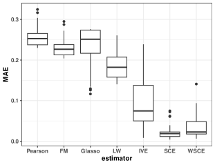
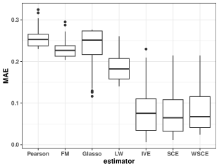
	Known	Unknown

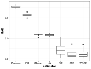
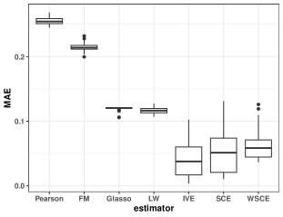
Figure 1: Boxplots of the mean absolute error (MAE) for the Pearson correlation matrix (Pearson), the estimator that uses factor models (FM), the glasso estimator (Glasso), the Ledoit-Wolf estimator (LW), and the IVE, SCE, and WSCE for 40 independent simulations. Estimators were evaluated in the fully simulated setting (FSS) and the setting of the TFR dataset (TFR). Left: the case when the means and variances are known. Right: the case when they are unknown and estimated by using the sample mean and variance. The errors of the IVE, SCE and WSCE are the lowest, with the SCE and WSCE outperforming the IVE when the means and variances are known.

4.3 Performance with varying dimensions of the data

We now describe the performance of the WSCE for different values of $d$.

Description

We consider the TFR setting with known mean and variance parameters. We selected subsets of the data of sizes $d=14,32,65,115,195$. These subsets are created by cumulatively including countries in Southern and Middle Africa, Eastern Africa, Western and Northern Africa, Asia and America, and all other countries, respectively.

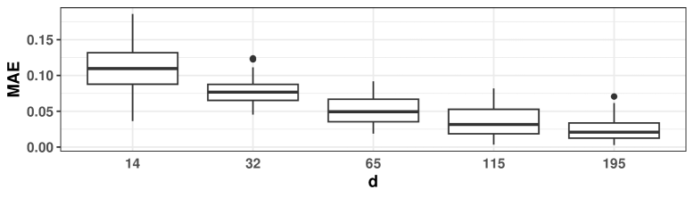
Figure 2: Boxplot of the mean absolute error (MAE) of the WSCE with different values of $d$, repeated for 40 independent simulations. The values of $d$ correspond to the number of countries in the following regions (added cumulatively): Southern and Middle Africa, Eastern Africa, Western and Northern Africa, Asia and America, the remaining countries in the dataset.

Results

The results are shown in Figure 2. $T=11$ was fixed, and $40$ different datasets were simulated independently for each value of $d$. The mean absolute error decreases with the number of countries, $d$. This was expected due to the consistency in $d$ of the parameters (Theorem 3.4). In other words, adding more countries to the dataset improved the performance of the WSCE.

4.4 Performance under model misspecification and the presence of missing values

Settings

Here, we study the impact of model misspecification on our estimators. We replace $R$ by $R_{\text{miss}}$ in Equation (13), where

$$R_{miss} =\xi R(\alpha,\beta,\delta)+(1-\xi)\tilde{R},$$

with $\xi\in[0,1]$, $R(\alpha,\beta,\delta)$ denoting the correlation structure from the TFR setting and $\tilde{R}$ being simulated using an additional matrix $F_{miss}$ from the FSS setting, which is not given to the model. Thus, the model assumptions hold when $\xi=0$, and the correlation structure does not depend on the observed covariates when $\xi=1$.

In the TFR dataset, the values of the standardized errors are missing for countries that have not yet entered phase II or III of the model of Alkema et al. (2011a). Thus, in this scenario, we consider two settings: one without missing values and the other one with missing values. In the latter scenario, we set the values of $Y_{t}$ that were missing in the TFR dataset to be missing. The IVE, SCE and WSCE need to be adapted under the presence of missing values. The corresponding procedure is described in Appendix E.

Results

The results are shown in Figure 3. Ten independent datasets were simulated for each value of $\xi$ and estimators were evaluated on the scale of the correlation matrix. The SCE and the WSCE perform similarly and outperform the other estimators in the scenarios that are not too far away from the model assumptions. As expected, the performances of both the SCE and the WSCE deteriorate when the value of $\xi$ increases, meaning that the scenario gets further away from the model assumptions. However, when the scenario is very different from the model assumptions ($\xi>0.5$), the WSCE outperforms the SCE and performs at least as well as the other estimators.

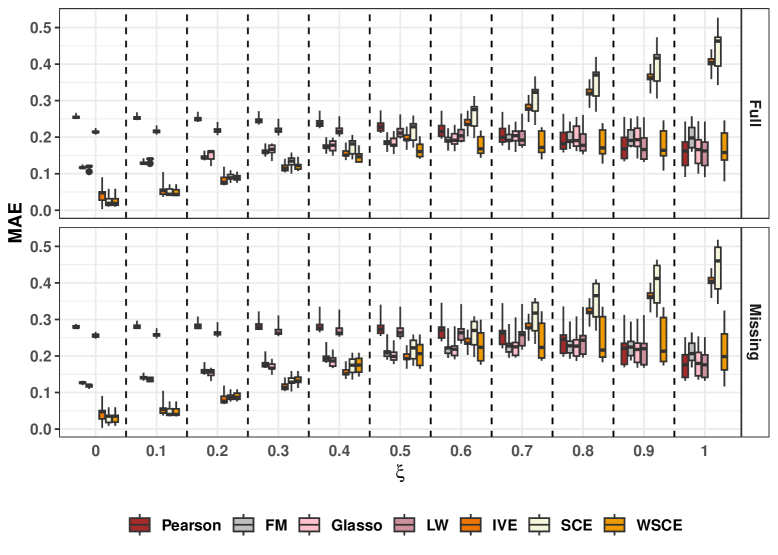
Figure 3: Boxplots of the mean absolute error (MAE) of the Pearson correlation matrix (Pearson), the Ledoit-Wolf estimator (LW), the estimator that uses factor models (FM), the glasso estimator (Glasso), IVE, SCE and WSCE, for $\xi=0,0.1,\dots,0.9,1$. 10 independent simulations were calculated by adding additional structure to the correlation, which is unknown and randomly simulated. At $\xi=1$, the correlation structure does not depend on the observed covariates. Full: no missing values. Missing: values that were missing in the original dataset were also set to be missing. The results do not change much between these two settings. This indicates that the missing-value imputation used is quite robust.

5 Covariance estimates for the TFR dataset

In this section, we will study the TFR dataset. We start by describing the data in detail. Then, we calculate our estimators with and without interaction terms, and we finish by performing model selection.

5.1 TFR data description

As described in Section 2.1, we want to estimate the covariance matrix of the total fertility rate (TFR) for 195 countries. Since we are in a Markov model with dependent observations, we estimate the covariance matrix of the TFR conditional on its preceding values, where the covariance matrix can vary with time. We assume that we are in the model described by Equation  (5).

Let us recall that in this model, the data $(Y_{1},\dots,Y_{T})$ denotes the TFR at time $1,\dots,T$. We fit the model described in Equation (9) with

$$R(\alpha,\beta,\delta)=\alpha_{A}F_{A}+\alpha_{B}F_{B}+\alpha_{C}F_{C}+\delta_{D}\Gamma(\beta_{D})^{-1}+\alpha_{E}I_{d},$$ (16)

where $(F_{A})_{i,j},(F_{B})_{i,j}$ are equal to 1 if country $i$ and $j$ have the same common colonizer or belong to the same UN region, respectively, $(F_{C})_{i,j}$ is always 1, and $\Gamma(\beta_{D})$ is described by Equation (6).

Table 1: The number of countries in phase I of the model of Alkema et al. (2011a) for each of the successive 5-year periods used in the TFR dataset. They are decreasing from the period 1950-1955, during which all countries were in phase I, to the period 2005-2010, during which all countries are no longer in phase I.

1950-1955	1955-1960	1960-1965	1965-1970	1970-1975	1975-1980
196	121	98	74	56	35
1980-1985	1985-1990	1990-1995	1995-2000	2000-2005	2005-2010
26	7	4	2	0	0

Selected countries

Vanuatu was reportedly colonized by two countries. This non-unique cluster membership could be modelled by splitting the common colonizer covariate into multiple distinct covariates for each respective cluster. However, this would unreasonably increase the number of parameters that we would need to estimate. Thus, we removed the corresponding variable and worked with the remaining $d=195$ countries.

Missing values

We aim at estimating the covariance matrix for country pairs where both countries have entered either phase II or III of the model of Alkema et al. (2011a). The TFR values of the countries that are still in phase I are thus treated as missing values. As time passes, more countries go from phase I to phase II. Thus, the number of missing values changes between the observations. We give the number of countries that are in phase I at each time period in Table 1. The values of the standardized errors $\varepsilon_{t,j}$, that are used to estimate the covariance matrix, are assumed to be missing at random everywhere. Thus, covariance estimation is appropriate on the marginal distribution of the non-missing values (Rubin, 1976; Seaman et al., 2013).

Remark 5.1.

Once a country leaves phase I, it will no longer return to it. Thus, the missing value structure is monotone and by construction the values of $\varepsilon_{t,j}$ are missing at random everywhere because the observed data vector directly implies the positions of the missing and observed data.

5.2 Covariance without interaction

In this section we compute the SCE by estimating the parameters of Equation (16).

Impact of the covariate

We introduce the concept of average effects to compare the effects of the different covariates in the model. The average effect of a covariate is the average correlation in the data that is due to this covariate. For direct effects, this corresponds to the value of the linear coefficients ($"$common colonizer$"$, $"$same region$"$). For the contiguity effect, we take the overall mean effect of country pairs which are direct neighbors of each other,

$$\eta_{contig}=\frac{1}{\sum_{i\neq j}M_{i,j}}\sum_{i\neq j\text{{ s.t. }}M_{i,j}=1}\delta_{D}\Gamma(\beta_{D})_{i,j}^{-1}.$$

Remark 5.2.

$\eta_{contig}$ is not equal to $\delta_{D}$ because, contrary to the values of $F_{A}$ or $F_{B}$, $\Gamma(\beta_{D})_{i,j}^{-1}$ is not always equal to $0$ or $1$.

The rationale is that if one adds all the pertinent coefficients for a given covariate, one gets the mean of the correlations for data points that have this covariate in common. For instance:

$$\alpha_{B}+\eta_{contig},$$

gives the mean of the estimated correlations of countries that are neighbors and in the same region, but not with the same colonizer.

The estimated average effects are given in Table 2.

5.3 Interaction effects and model selection

We can see in Table 2 that at least two effects needed to overlap for countries to have a correlation higher than 0.2. This was not the case in Fosdick and Raftery (2014), where, e.g., the contiguity effect alone accounted for a correlation of 0.26 for all country pairs with TFRs below 5. We wanted to check if there were interaction effects. Indeed the neighborhood effect, for instance, may be different if you are in the same region or not.

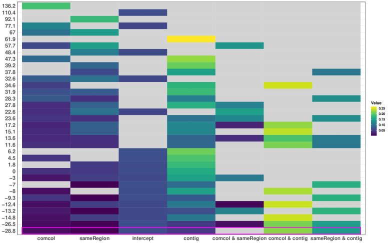
Figure 4: On the $y$-axis: values of the BIC for all 35 models tested; the BIC is centered such that the model which includes all but interaction effects shows a value of 0; grey squares indicate effects that are not included in their respective model; on the $x$-axis: different average effects; we can see that only models which include interaction effects have a lower BIC than this model; the model with the lowest BIC set only the combined effect of the $"$regional$"$ and $"$common-colonizer$"$ covariates to 0.

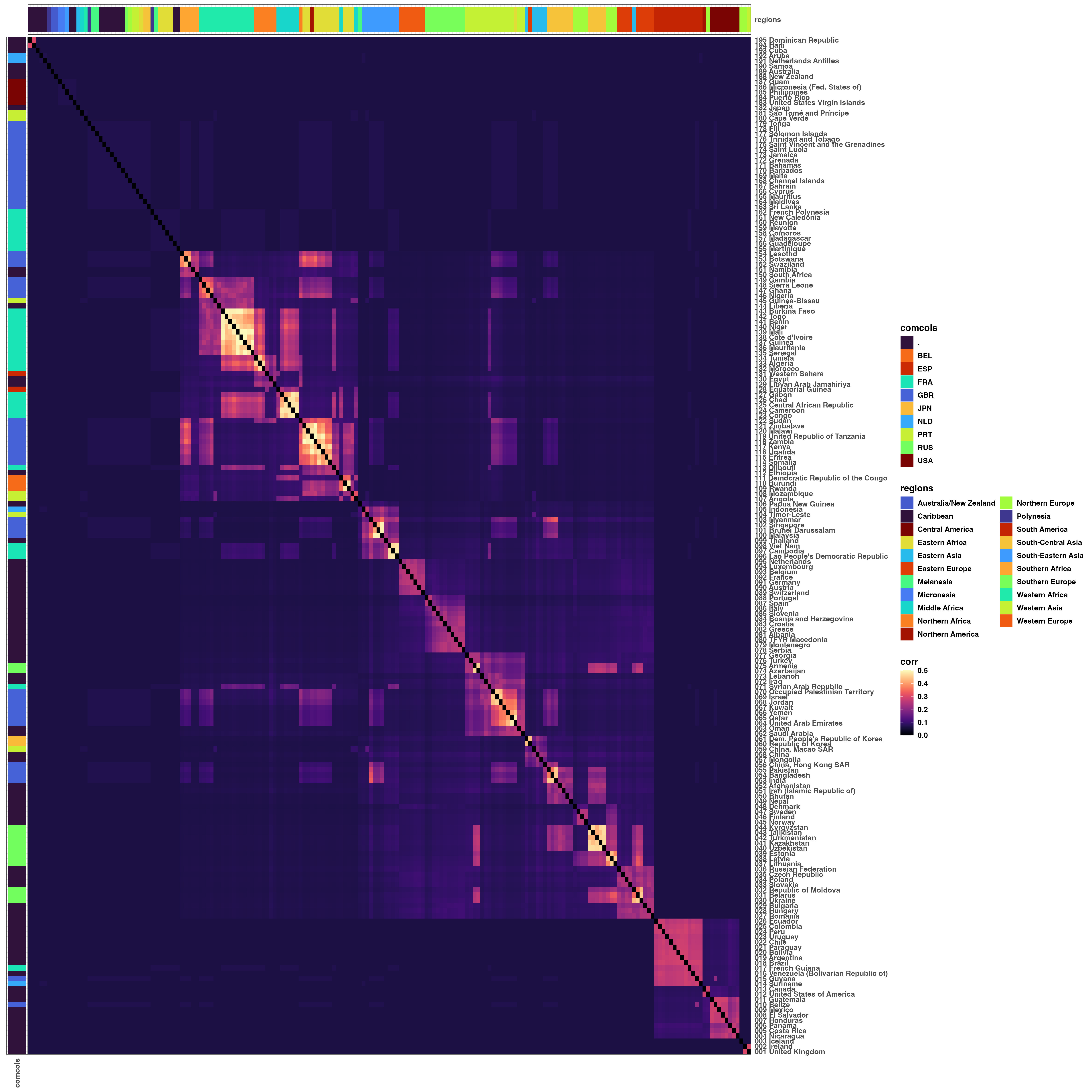
Figure 5: A heatmap of the correlation matrix calculated from the WSCE (diagonal entries were set to 0 to improve the visualization); on the x-axis: colonizers (countries with no colonizer were set to belong to colonizer $"$.$"$); on the y-axis: regions; Countries are particularly correlated if they are close to each other and are either in the same region or share the same common colonizer. The matrix was sorted using the order given by hierarchical clustering with the Ward distance on the dissimilarity matrix $1-\hat{R}_{\text{WSCE}}$, using the option ”$h$-clust” in the ”corrplot” package (Wei and Simko, 2021).

Table 2: Average effects of the model in which all effects are included. All effects were rounded to the third decimal place.

	comcol	sameRegion	intercept	contig
	0.038	0.044	0.06	0.162

Thus, in addition to the intercept, $"$common colonizer$"$, $"$same region$"$ and the spatial effect we add their interactions by adding random effects with correlation matrices equal to the Hadamard product of the correlation matrices of the individual effects. Martini et al. (2020) do that with covariance matrices but since we separate the variance from the correlation matrix estimation, we use correlation matrices instead.

We can include up to 3 interaction effects, with correlation matrices

$$F_{A,B}=F_{A}\odot F_{B},\text{ common colonizer and same region effect},$$

$$F_{A,D}=F_{A}\odot\Gamma(\beta_{D})^{-1},\text{ common colonizer and spatial effect,}$$

$$F_{B,D}=F_{B}\odot\Gamma(\beta_{D})^{-1},\text{ same region and spatial effect}.$$

This gives up to 8 effects. We select which effect we should include by computing the BIC for each of the possible $128=2^{8}$ models. However, we exclude interaction effects whenever one of their individual component effects is excluded. This reduces the scope of our model selection to 35 models, the results of which are plotted in Figure 4.

The BIC was centered in the base model described in Equation (16). Interestingly, the only models with a better (lower) BIC than the base model are the ones that do include interaction effects. This is in agreement with Fosdick and Raftery (2014), which kept all these effects, but did not try to add interactions. The model with the lowest BIC is the model that includes all but one interaction effect, the effect that accounts for the interaction between $"$common colonizer$"$ and the $"$same region$"$ effect.

Just as for the previous model, we compared the average effects in this model. For interactions between direct effects (common colonizer and same region), the average effect is the coefficient $\alpha_{A,B}$. For interaction effects that involve the contiguity effect, we take the mean effect of all pairs of countries that are neighbors and in the same region (resp., have the same colonizer):

$$\eta_{contig,B}=\frac{1}{\sum_{i\neq j}(F_{B}\odot M)_{i,j}}\sum_{i\neq j\text{{ s.t. }}M_{i,j}=1\;\&\;(F_{B})_{i,j}=1}\alpha_{B,D}(F_{B}\odot\Gamma(\hat{\beta}_{\text{SCE}})^{-1})_{i,j}.$$

Table 3: Average effects of the model chosen in Figure 4, in which all effects and their interactions, but the interaction of the $"$common colonizer$"$ and the $"$same region$"$ effect are included. All effects but the regional effect were rounded to the third decimal place.

	comcol	sameRegion	intercept	contig	comcol and contig	sameRegion and contig
	0.008	2e-06	0.061	0.045	0.218	0.146

Table 3 gives the average effects of the selected model. Effects are much higher when two attributes overlap.

The correlation matrix obtained with these coefficients is plotted in Figure 5. Except for some clusters of countries, the TFRs of two countries are mostly estimated to not be highly correlated, given their previous TFRs.

To check if we do not miss correlations that may come from an effect that is not included in the model, we computed the WSCE. However, it was equal to the SCE. In our simulation settings this corresponds to the case where our model assumptions were correct. Thus, we can find no evidence against our model assumptions.

6 Discussion

We introduced the structured covariance estimator (SCE) and the weighted structured covariance estimator (WSCE), estimators for large covariance matrices in the presence of pairwise covariates. We showed consistency and asymptotic normality of these estimators in the dimension of the data and in the number of data points and gave a procedure for estimating their confidence regions, under mild assumptions. Furthermore, we tested our estimators in scenarios in which some part of our model was misspecified, where the WSCE performed well.

We incorporated pairwise information into the covariance matrix estimation by modelling the standardized errors as a sum of weighted and standardized random effects. A very different approach from ours would be to penalize the estimator of the covariance matrix directly. This was done by Liu et al. (2014), and in a Bayesian way by Azose and Raftery (2018), both of which use a weight matrix to penalize individual matrix entries. However, this requires direct estimation of all parameters of the covariance matrix, of which there are $195\times 194/2=18,915$ in our case. We do not need to do this in our model, where we only require efficient estimation of a small number of parameters. In fact, Azose and Raftery (2018) pointed out that the high dimension of their parameter space made it impractical for them to carry out an MCMC simulation in their Bayesian setting. In contrast, an extension of our method to the Bayesian paradigm would be straightforward, since we only need to simulate a vector of dimension 6.

The initial value of our estimator, the IVE, performed well in our simulation study. The WSCE is an asymptotically optimal interpolation between the SCE and the Pearson correlation matrix, as long as the underlying distribution of the data is Gaussian. However, if the distribution is very different from a Gaussian distribution, it might perform suboptimally. In this case, one could instead use a linear interpolation between the IVE and the Pearson correlation matrix, since the IVE is consistent and asymptotically normal if our correlation structure holds, but the data are non-Gaussian.

There is also the question of whether we should be using the Pearson correlation matrix in constructing the WSCE. We obtained decent results even in scenarios far from our model assumptions, but note that the Pearson correlation matrix is known to not behave well in settings with small sample size and a high number of variables. Depending on the setting, one can decide to use a more adapted estimator in the construction of the WSCE, such as the Ledoit-Wolf estimator or Glasso for instance.

A similar argument can be made for our mean- and variance estimators: we used the fact that accurate estimates of the mean and variance of the data were already provided. This is convenient. but not necessary. In cases where these estimates are not provided we recommend estimating the mean-, variance-, and correlation structure jointly if computationally feasible.

Finally, the WSCE could be adapted to very general settings such as generalized linear models (GLMs), in a similar vein to Bonat and Jørgensen (2016).

The name of the WSCE refers to the fact that we have a weighted combination of correlation structures defined via known covariates. It is not to be confused with techniques that have similar names, but only focus on the estimation of one given matrix structure, such as Burg et al. (1982); Sun et al. (2016); Lopuhaä et al. (2023).

Acknowledgements The authors would like to thank Daniel Suen for recommending the re-use of the initialization step of the estimator in the bootstrapping procedure (instead of reevaluating it in each sample that was simulated), and Julie Josse for her recommendation of Josse and Husson (2016).

Raftery’s research was supported by NIH grant R01 HD-070936, the Fondation des Sciences Mathématiques de Paris (FSMP), and Université Paris Cité (UPC). He thanks the Laboratoire MAP5 at UPC for warm hospitality.

Supplementary material Contains Appendix A (derivatives of the likelihood), Appendix B (proofs), Appendix C (details on the algorithm), Appendix D (alternative model justifications), and Appendix E (simulation settings details).

References

- Aguilar and West (2000) Aguilar, O. and M. West (2000). Bayesian dynamic factor models and portfolio allocation. Journal of Business & Economic Statistics 18(3), 338–357.
- Alkema et al. (2011a) Alkema, L., A. E. Raftery, P. Gerland, S. J. Clark, F. Pelletier, T. Buettner, and G. K. Heilig (2011a). Probabilistic projections of the total fertility rate for all countries. Demography 48(3), 815–839.
- Alkema et al. (2011b) Alkema, L., A. E. Raftery, P. Gerland, S. J. Clark, F. Pelletier, T. Buettner, and G. K. Heilig (2011b). Probabilistic projections of the total fertility rate for all countries, Online Resource 1. Demography 48(3), 815–839.
- Anderson (1973) Anderson, T. W. (1973). Asymptotically efficient estimation of covariance matrices with linear structure. The Annals of Statistics 1(1), 135–141.
- Azose and Raftery (2018) Azose, J. J. and A. E. Raftery (2018). Estimating large correlation matrices for international migration. The annals of applied statistics 12(2), 940.
- Barnard et al. (2000) Barnard, J., R. McCulloch, and X.-L. Meng (2000). Modeling covariance matrices in terms of standard deviations and correlations, with application to shrinkage. Statistica Sinica 10(4), 1281–1311.
- Bates et al. (2024) Bates, D., M. Maechler, and M. Jagan (2024). Matrix: Sparse and Dense Matrix Classes and Methods. R package version 1.7-0.
- Bernardo et al. (2003) Bernardo, J., M. Bayarri, J. Berger, A. Dawid, D. Heckerman, A. Smith, and M. West (2003). Bayesian factor regression models in the “large p, small n” paradigm. Bayesian statistics 7, 733–742.
- Besag and Kooperberg (1995) Besag, J. and C. Kooperberg (1995). On conditional and intrinsic autoregressions. Biometrika 82(4), 733–746.
- Besag et al. (1991) Besag, J., J. York, and A. Mollié (1991). Bayesian image restoration, with two applications in spatial statistics. Annals of the institute of statistical mathematics 43, 1–20.
- Bonat and Jørgensen (2016) Bonat, W. H. and B. Jørgensen (2016). Multivariate covariance generalized linear models. Journal of the Royal Statistical Society Series C: Applied Statistics 65(5), 649–675.
- Broyden (1970) Broyden, C. G. (1970). The convergence of a class of double-rank minimization algorithms 1. general considerations. IMA Journal of Applied Mathematics 6(1), 76–90.
- Burg et al. (1982) Burg, J. P., D. G. Luenberger, and D. L. Wenger (1982). Estimation of structured covariance matrices. Proceedings of the IEEE 70(9), 963–974.
- Cavazani de Freitas et al. (2022) Cavazani de Freitas, L. A., L. de Oliveira Carlos, A. C. Ligocki Campos, and W. H. Bonat (2022). Hypothesis tests for multiple responses regression: effect of probiotics on addiction and binge eating disorder. arXiv e-prints, arXiv–2208.
- Cheng and Higham (1998) Cheng, S. H. and N. J. Higham (1998). A modified Cholesky algorithm based on a symmetric indefinite factorization. SIAM Journal on Matrix Analysis and Applications 19(4), 1097–1110.
- Chiu et al. (1996) Chiu, T. Y., T. Leonard, and K.-W. Tsui (1996). The matrix-logarithmic covariance model. Journal of the American Statistical Association 91(433), 198–210.
- Christensen and Amemiya (2003) Christensen, W. F. and Y. Amemiya (2003). Modeling and prediction for multivariate spatial factor analysis. Journal of Statistical planning and inference 115(2), 543–564.
- Erdős and Rényi (1959) Erdős, P. and A. Rényi (1959). On random graphs i. Publ. Math. 6(290-297), 18.
- Fan et al. (2016) Fan, J., Y. Liao, and H. Liu (2016, 03). An overview of the estimation of large covariance and precision matrices. The Econometrics Journal 19(1), C1–C32.
- Fletcher and Reeves (1964) Fletcher, R. and C. M. Reeves (1964). Function minimization by conjugate gradients. The computer journal 7(2), 149–154.