$\ell_{0}$-Regularized Sparse Coding-based Interpretable Network for Multi-Modal Image Fusion

Abstract

Multi-modal image fusion (MMIF) enhances the information content of the fused image by combining the unique as well as common features obtained from different modality sensor images, improving visualization, object detection, and many more tasks. In this work, we introduce an interpretable network for the MMIF task, named FNet, based on an $\ell_{0}$-regularized multi-modal convolutional sparse coding (MCSC) model. Specifically, for solving the $\ell_{0}$-regularized CSC problem, we develop an algorithm unrolling-based $\ell_{0}$-regularized sparse coding (LZSC) block. Given different modality source images, FNet first separates the unique and common features from them using the LZSC block and then these features are combined to generate the final fused image. Additionally, we propose an $\ell_{0}$-regularized MCSC model for the inverse fusion process. Based on this model, we introduce an interpretable inverse fusion network named IFNet, which is utilized during FNet’s training. Extensive experiments show that FNet achieves high-quality fusion results across five different MMIF tasks. Furthermore, we show that FNet enhances downstream object detection in visible-thermal image pairs. We have also visualized the intermediate results of FNet, which demonstrates the good interpretability of our network. .

I Introduction

Multi-modal image fusion (MMIF) is an active area of research for many years. In MMIF, the aim is to integrate information captured using different modality sensor images into a single fused image, offering enhanced information content compared to individual single-modality sensor images. This improves visualization and interpretation, making the fused image more appropriate for downstream tasks like object detection, segmentation, disease diagnosis, and more [1, 2].

In MMIF, different modality sensors capture images of the same scene, collecting some common image features shared across all the modalities. Additionally, each modality acquires its own unique image features. Some recent MMIF methods [3, 4, 5] have been designed to first separate the unique and common features in the source images and then generate the fused image by integrating these features. To separate the unique and common features, [3, 5] solved a multi-modal dictionary learning model using the alternating direction method of multipliers (ADMM) [6]. However, this approach is time-consuming and not very effective for large-scale data. To overcome the limitation of the optimization-based method, Deng et al. [4] designed an interpretable deep neural network (DNN), named CUNet, based on an $\ell_{1}$-regularized multi-modal convolutional sparse coding (MCSC) model. CUNet uses learned convolutional sparse coding (LCSC) blocks to estimate the unique and common features. Though CUNet appears effective for separating the unique and common features, there still remains an issue with the LCSC block, which is designed by unrolling a convolutional extension of the iterative shrinkage thresholding algorithm (ISTA) [7] to estimate the $\ell_{1}$-regularized sparse features. ISTA uses a soft thresholding function, which nullifies the features with absolute values smaller than a threshold value and thus promotes sparsity. However, the soft thresholding function also reduces the magnitude of the features with higher absolute values and overpenalizes them. This makes the magnitude of the ISTA-based sparse estimation lower than the $\ell_{0}$-regularized optimal sparse estimation [8]. Constraining the unique and common features to be $\ell_{0}$-regularized can overcome this problem [9]. Moreover, for the MMIF task, where the ground truth fused image is not available, considering an inverse fusion process proves effective [10, 11]. In the inverse fusion process, the fused image is separated back into its source images, and as the quality of these separated images is dependent on the quality of the fused image, constraining them to be similar to the original source images helps enforce the generation of a higher-quality fused image.

This work introduces a novel $\ell_{0}$-regularized MCSC model to address the MMIF task. In this model, we represent each modality source image as a combination of $\ell_{0}$-regularized unique and common sparse features. Based on this model, a DNN named FNet is developed to solve the MMIF task. Due to such a model-based design, FNet has the benefits of both model-based and DNN. Model-based methods promote prior domain knowledge and interpretability of the underlying physical process, whereas DL methods are very efficient in learning from large-scale data [12]. Since no existing work has designed a DNN to solve the $\ell_{0}$-regularized CSC problem, we propose a novel learnable $\ell_{0}$-regularized sparse coding (LZSC) block. To design the LZSC block, we first develop an iterative algorithm for solving the $\ell_{0}$-regularized CSC problem and then unroll this algorithm into our learnable LZSC block. In FNet, first, the unique and common features are separated from different modality source images using our proposed LZSC blocks. Then, these features are integrated to get the final fused image. In our work, constraining the unique and common features to be $\ell_{0}$-regularized solves the fundamental formulation of sparse coding and estimates accurate sparse features. Moreover, we propose a novel MCSC model to represent the inverse fusion process. In this model, we represent the fused image as a combination of $\ell_{0}$-regularized sparse features corresponding to the different modality source images. Based on this model, we design an interpretable inverse fusion network named IFNet. Given the fused image, IFNet first estimates the features corresponding to the source images using our LZSC blocks and then obtains the source images using the convolution operation. We utilize IFNet in the training of FNet. Constraining the decomposed source images obtained by IFNet to be similar to the original source images improves the scene representation quality in the fused image.

Our primary contributions can be outlined below:

1. We develop a novel algorithm unrolling-based learnable LZSC block to solve the $\ell_{0}$-regularized CSC problem. This is the first learnable block to solve the $\ell_{0}$-regularized CSC problem to the best of our awareness.

2. We introduce an MCSC model to address the MMIF task. In this model, we represent each modality source image as a combination of $\ell_{0}$-regularized unique and common sparse features. Based on this model and our LZSC block, we propose an interpretable fusion network named FNet.

3. We introduce an MCSC model for the inverse fusion process. In this model, we represent the fused image as a combination of $\ell_{0}$-regularized sparse features corresponding to the different modality source images. Based on this model and our LZSC block, we propose an interpretable inverse fusion network named IFNet, which is utilized in the training of FNet.

4. FNet achieves leading results on five MMIF tasks: visible and infrared (VIS-IR), visible and near-infrared (VIS-NIR), computed tomography and magnetic resonance imaging (CT-MRI), positron emission tomography and MRI (PET-MRI), and single-photon emission computed tomography and MRI (SPECT-MRI) image fusion. Moreover, FNet also facilitates downstream object detection in visible-thermal image pairs.

The remaining paper is structured as follows. In Section II, we review the sparse coding methods and prior works on the MMIF task and the inverse fusion process. Section III describes our proposed LZSC block, FNet, IFNet, and the training process in detail. We conduct extensive experiments in Section IV to validate our proposed method. Finally, Section V concludes the paper.

II Background

First, we review the sparse coding methods. Next, we discuss the prior works on the MMIF task. Finally, we review the inverse fusion process.

II-A Sparse Coding

Sparse coding (SC) is a widely used technique to select the salient features in a signal or image [13, 14, 4]. The classical SC method represents a signal $x\in\mathbb{R}^{n\times 1}$ encoded into its sparse representation $z\in\mathbb{R}^{m\times 1}$ using a learned dictionary $D\in\mathbb{R}^{n\times m}$. The sparse representation $z$ is estimated by solving the $\ell_{0}$-regularized problem,

$$\underset{z}{\mathrm{Argmin}}\>\frac{1}{2}||\>x-Dz||_{2}^{2}+\lambda||z||_{0}$$ (1)

By imposing the $\ell_{0}$ regularization, $z$ is enforced to have only the salient features as the non-zero elements. However, Eqn. 1 is a non-convex and NP-hard formulation [15]. A popular way to address this problem is to relax the non-convex $\ell_{0}$ pseudo-norm with the convex $\ell_{1}$ norm [16]. But only under certain conditions, the $\ell_{1}$-regularized sparse estimation matches with the $\ell_{0}$-regularized solution [17]. Solving the original $\ell_{0}$-regularized problem can be more effective in many cases. Blumensath et al. [18] proposed an iterative hard thresholding algorithm (IHTA) to solve Eqn. 1, and [19] modified IHTA to a normalized IHTA (NIHTA) for better convergence. Following NIHTA, the iteration step for updating $z$ is,

$$z^{k+1}=H_{\theta}\Big{(}z^{k}-\mu D^{T}\Big{(}Dz^{k}-x\Big{)}\Big{)}$$ (2)

where $z^{k}$ is the sparse estimation at $k^{th}$ iteration and $\mu$ is the step size. $H_{\theta}(\cdot)$ is the hard thresholding function with threshold value $\theta$ defined as,

$$H_{\theta}(x)=\begin{cases}\>0&\text{\>if\>\>}|x|\leq\theta\\ \>x&\text{otherwise}\end{cases}$$ (3)

Fig. 1-(a) shows the $H_{\theta}(\cdot)$ function, which promotes a sparse solution by nullifying the input with absolute values smaller than $\theta$. However, traditional iterative approaches take many iterations to solve the sparse estimation, and an algorithm unrolling-based neural network can have better estimation accuracy [20]. Also, network formulation can facilitate task-specific optimization. Based on the IHTA algorithm, [21, 20] modeled feed-forward neural networks for solving the classical SC problem.

Generally, solving the classical SC problem is computationally intensive due to the matrix multiplication operation. Because of this, for high-resolution images, most methods split the image into overlapped patches, and each patch is processed independently to estimate the sparse representations and then aggregated using an averaging operation. Since the correlation between the patches is not considered, the estimation accuracy is poor. To address this issue, the convolutional sparse coding (CSC) method was proposed in [22, 23]. CSC models the complete image as a sum over convolutional sparse representations (CSRs). For $\ell_{0}$-regularized CSC, the matrix multiplication in Eqn. 1 is substituted with the convolutional operation,

$$\underset{z}{\mathrm{Argmin}}\>\frac{1}{2}||\>x-D(z)||_{2}^{2}+\lambda||z||_{0}$$ (4)

where $D(\cdot)$ is a convolution operation. Rodríguez [24] solved the $\ell_{0}$-regularized convolutional sparse coding (CSC) problem with an escape strategy-based iterative algorithm. However, there is no work that designed a neural network to solve the $\ell_{0}$-regularized CSC problem.

The existing learning-based CSC method [16] solves the $\ell_{1}$-regularized CSC problem. Sreter et al. [16] introduced a learned convolutional sparse coding (LCSC) block by unrolling a convolutional extension of ISTA [7]. The iteration steps of ISTA are similar to Eqn. 2, only $H_{\theta}(\cdot)$ is replaced by the soft thresholding function, $S_{\theta}(\cdot)$ given by,

$$S_{\theta}(x)=max(|x|-\theta,0)\>sgn(x)$$ (5)

$sgn(\cdot)$ denotes the sign function. As illustrated in Fig. 1-(b), $S_{\theta}(\cdot)$ also nullifies the smaller input values like $H_{\theta}(\cdot)$. But, it also reduces the input with higher absolute values and thus over-penalizes them. This makes the magnitude of the sparse estimation lower than the $\ell_{0}$-regularized optimal sparse solution [8], which is an inherent limitation of the ISTA-based methods. Due to this, the ISTA-based LCSC block [16] has limited performance in estimating the sparse solution.

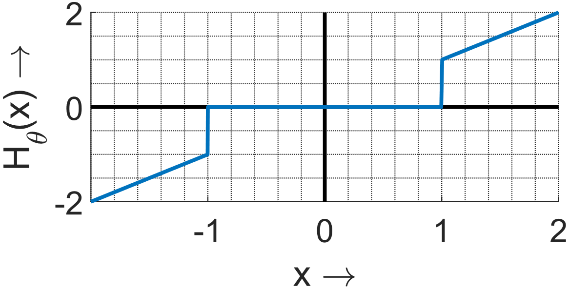
((a))

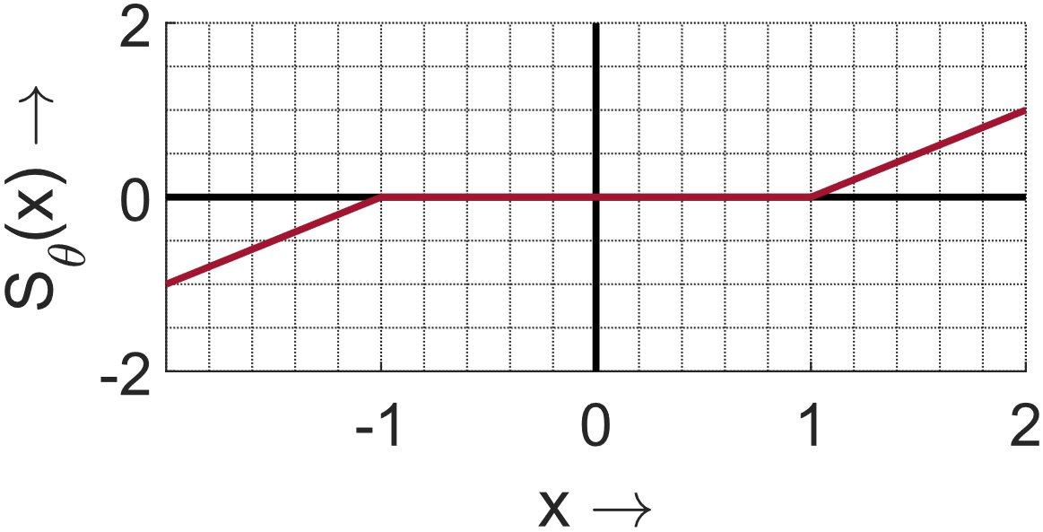
((b))

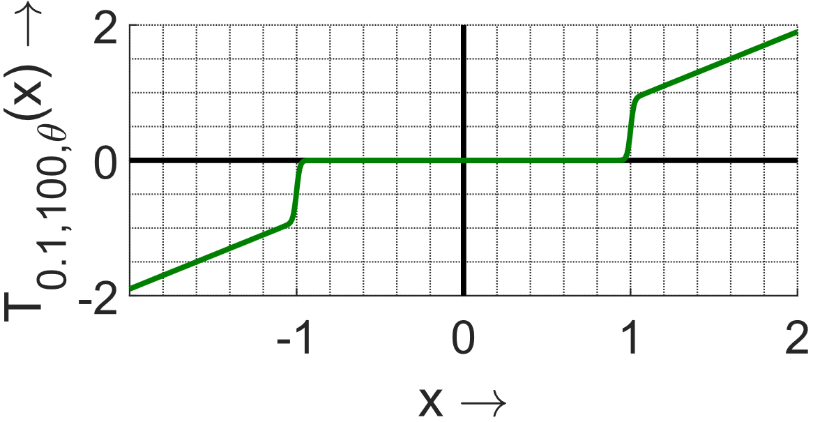
((c))

Figure 1: Different thresholding functions with threshold value $\theta$ as $1$. (a) Hard thresholding function, $H_{\theta}(\cdot)$, (b) Soft thresholding function, $S_{\theta}(\cdot)$, (c) Sigmoidal thresholding function, $T_{0.1,100,\theta}(\cdot)$.

To address the above-mentioned issues, we introduce a learnable $\ell_{0}$-regularized sparse coding (LZSC) block, which is developed by unrolling an iterative algorithm that solves the $\ell_{0}$-regularized CSC problem in Eqn. 4. The iterative algorithm is designed by incorporating Nesterov’s momentum [25] with a convolutional extension of the NIHTA steps in Eqn. 2. However, the $H_{\theta}(\cdot)$ function in Eqn. 2 is a discontinuous function, and training neural networks with such a function is generally difficult [21]. To address this issue, we use a sigmoidal thresholding function proposed in [26],

$$T_{\alpha,\gamma,\theta}(x)=\frac{|x|-\alpha\theta}{1+e^{-\gamma(|x|-\theta)}}$$ (6)

where $\gamma$ is a parameter controlling the speed of the threshold transition, and $\alpha\in[0,1]$ indicates the additive adjustment that is made for input with larger absolute values. In the limiting cases, $T_{1,\infty,\theta}(\cdot)$ approximates $S_{\theta}(\cdot)$, and $T_{0,\infty,\theta}(\cdot)$ approximates $H_{\theta}(\cdot)$. Fig. 1-(c) shows $T_{0.1,100,\theta}(\cdot)$, which has a smoother transition compared to $H_{\theta}(\cdot)$ and unlike $S_{\theta}(\cdot)$, imposes very small penalty for the larger input values. Instead of $H_{\theta}(\cdot)$, we use this $T_{0.1,100,\theta}(\cdot)$ for better network training. Our LZSC block-based method has superior performance than the existing LCSC block-based method [16] for the MMIF task.

II-B Prior Works on MMIF

In this era of DL, the methods to solve the MMIF task can be categorized into two primary groups: pure DL-based models [27, 28, 1, 29, 30, 31, 32, 33, 34, 11], and algorithm unrolling-based models [35, 4]. Pure DL-based MMIF models typically utilize convolutional neural networks (CNNs) [27, 28, 29, 32], transformers [1, 31, 30, 33, 34, 11], and generative adversarial networks (GANs) [2] to construct a deep neural network to learn the mapping between the fused image and the source images. Although pure DL-based models have the potential to produce high-quality fused images, they lack interpretability in the underlying fusion process.

Whereas algorithm unrolling-based MMIF models [4, 35] derive inspiration from traditional algorithms and unroll an iterative algorithm into an interpretable deep neural network. LRRNet [35] decomposes the source images into sparse and low-rank components based on a low-rank representation model and then combines the components to get the fused image. However, while decomposing the source images, it does not consider the dependency across modalities. Deng et al. [4] proposed a multi-modal convolutional sparse coding (MCSC) model to represent the MMIF process. Based on this model, they designed an interpretable network named CUNet that first separates the unique and common features from the different modality source images and then combines the features to get the fused image. In CUNet, the unique and common features are estimated using the LCSC block [16] that solves an $\ell_{1}$-regularized CSC problem. However, as discussed in Section II-A, the LCSC block-based method has limitations in estimating the sparse solution, and solving the $\ell_{0}$ regularized optimization problem can be highly effective here. In our work, we propose an $\ell_{0}$ regularized MCSC model to represent the relationship between different modalities, and based on this model and our LZSC block, propose an interpretable MMIF network named FNet. Moreover, for the MMIF task, where the ground truth fused image is not available, considering an inverse fusion process can be very effective, which we discuss in the next subsection.

II-C Inverse Fusion Process

In DL-based MMIF methods, one line of works [10, 11] considers an inverse fusion process, where the fused image is decomposed into the source images. As the quality of the decomposed source images is dependent on the quality of the fused image, constraining them to be similar to the original source images helps enforce the fused image to contain maximum information from the source images. However, for the inverse fusion task, [10, 11] used purely DL-based networks where interpretability of the underlying inverse fusion process is absent. In our work, we also consider an inverse fusion network named IFNet in the training of our proposed FNet to improve the fused image quality. However, unlike other inverse fusion networks, our IFNet is developed based on a novel $\ell_{0}$ regularized MCSC model. Such a model-based development gives interpretability of the inverse fusion process. Incorporating IFNet into the training of FNet significantly improves the performance in the MMIF task.

III Proposed Method

III-A Problem Statement

In the MMIF process, different modality sensors capture the images of the same scene, which leads to the sharing of some common image features. However, since different modality sensors are used, the images also contain modality-specific unique features. The fused image can be obtained by combining these unique and common features. We consider two modalities of source images: $I_{1}\in\mathbb{R}^{H\times W\times 1}$ and $I_{2}\in\mathbb{R}^{H\times W\times 1}$, and fused image $I_{f}\in\mathbb{R}^{H\times W\times 1}$. $H$ and $W$ are the image height and width, respectively. The source images $I_{1}$ and $I_{2}$ share the same common feature $c\in\mathbb{R}^{H\times W\times K}$, where $K$ is the feature channel dimension. Moreover, $I_{1}$ and $I_{2}$ have their unique features $u_{1}\in\mathbb{R}^{H\times W\times K}$ and $u_{2}\in\mathbb{R}^{H\times W\times K}$ respectively. To select the salient features, we constrain $c$, $u_{1}$, and $u_{2}$ to be $\ell_{0}$-regularized. We propose the following $\ell_{0}$-regularized MCSC model to represent the fusion process,

$$\begin{split}&\mathrm{min}\>\>||c||_{0},\>\>||u_{1}||_{0},\>\>||u_{2}||_{0}\\ s.t.,\\ &I_{1}=D_{c_{1}}(c)+D_{u_{1}}(u_{1})\\ &I_{2}=D_{c_{2}}(c)+D_{u_{2}}(u_{2})\\ &I_{f}=\underbrace{G_{c}(c)}_{\begin{subarray}{c}\text{common part}\\ \text{from }I_{1}\text{ and }I_{2}\end{subarray}}+\underbrace{G_{u_{1}}(u_{1})}_{\begin{subarray}{c}\text{unique part}\\ \text{from }I_{1}\end{subarray}}+\underbrace{G_{u_{2}}(u_{2})}_{\begin{subarray}{c}\text{unique part}\\ \text{from }I_{2}\end{subarray}}\end{split}$$ (7)

where $D_{c_{1}}(\cdot)$, $D_{u_{1}}(\cdot)$, $D_{c_{2}}(\cdot)$, $D_{u_{2}}(\cdot)$, $G_{c}(\cdot)$, $G_{u_{1}}(\cdot)$ and $G_{u_{2}}(\cdot)$ denote learnable convolution operations. Now, given the source images $I_{1}$ and $I_{2}$, we solve the following optimization problem to estimate $c$, $u_{1}$, and $u_{2}$,

$$\begin{split}\underset{c,\>u_{1},\>u_{2}}{\mathrm{Argmin}}\>&\frac{1}{2}\Big{|}\Big{|}\>I_{1}-D_{c_{1}}(c)-D_{u_{1}}(u_{1})\Big{|}\Big{|}_{2}^{2}\\ +&\frac{1}{2}\Big{|}\Big{|}\>I_{2}-D_{c_{2}}(c)-D_{u_{2}}(u_{2})\Big{|}\Big{|}_{2}^{2}\\ +&\lambda_{c}||c||_{0}+\lambda_{u_{1}}||u_{1}||_{0}+\lambda_{u_{2}}||u_{2}||_{0}\end{split}$$ (8)

Following [4], we first update $u_{1}$ and $u_{2}$ by setting the value of $c$ to zero. Then, $c$ is updated by fixing $u_{1}$ and $u_{2}$. The steps are:

• $u_{i},i\in\{1,2\}$ is updated by solving the equation,

  $$\underset{u_{i}}{\mathrm{Argmin}}\>\frac{1}{2}\Big{|}\Big{|}\>I_{i}-D_{u_{i}}(u_{i})\Big{|}\Big{|}_{2}^{2}+\lambda_{u_{i}}||u_{i}||_{0}$$ (9)

• $c$ is updated by solving the equation,

  $$\begin{split}\underset{c}{\mathrm{Argmin}}\>&\frac{1}{2}\Big{|}\Big{|}\>\hat{I}_{1}-D_{c_{1}}(c)\Big{|}\Big{|}_{2}^{2}\\ +&\frac{1}{2}\Big{|}\Big{|}\>\hat{I}_{2}-D_{c_{2}}(c)\Big{|}\Big{|}_{2}^{2}+\lambda_{c}||c||_{0}\end{split}$$ (10)

  where $\hat{I}_{1}=I_{1}-D_{u_{1}}(u_{1})$ and $\hat{I}_{2}=I_{2}-D_{u_{2}}(u_{2})$. By channel-wise concatenating $\hat{I}_{1}$ and $\hat{I}_{2}$ to $\hat{I}_{1,2}\in\mathbb{R}^{H\times W\times 2}$, Eqn. 10 can be written as,

  $$\underset{c}{\mathrm{Argmin}}\>\frac{1}{2}\Big{|}\Big{|}\>\hat{I}_{1,2}-L_{c}(c)\Big{|}\Big{|}_{2}^{2}+\lambda||c||_{0}$$ (11)

  here $L_{c}(\cdot)$ is learnable convolution operation.

As discussed in Section II-C, employing an inverse fusion process in the training of the fusion network can enhance the fused image quality. Motivated by this, we consider an inverse fusion process where the fused image is separated into the source images. Since the fused image has information content from the different modality source images, we can represent the fused image as a combination of features from the source images. We consider that the fused image $I_{f}$ has the features $x_{1}\in\mathbb{R}^{H\times W\times K}$ and $x_{2}\in\mathbb{R}^{H\times W\times K}$ corresponding to the source images $I_{1}$ and $I_{2}$ respectively. To get the salient features, we constrain $x_{1}$ and $x_{2}$ to be $\ell_{0}$-regularized. We propose the following $\ell_{0}$-regularized MCSC model to represent the inverse fusion process,

$$\begin{split}&\mathrm{min}\>\>||x_{1}||_{0},\>\>||x_{2}||_{0}\\ s.t.,\\ &I_{f}=\underbrace{G_{x_{1}}(x_{1})}_{\begin{subarray}{c}\text{from }I_{1}\end{subarray}}+\underbrace{G_{x_{2}}(x_{2})}_{\begin{subarray}{c}\text{from }I_{2}\end{subarray}}\\ &I_{1}=D_{x_{1}}(x_{1})\\ &I_{2}=D_{x_{2}}(x_{2})\end{split}$$ (12)

where $G_{x_{1}}(\cdot)$, $G_{x_{2}}(\cdot)$, $D_{x_{1}}(\cdot)$ and $D_{x_{2}}(\cdot)$ denote learnable convolution operations. Given the fused image $I_{f}$, we estimate $x_{1}$ and $x_{2}$ by solving the follwing optimization problem,

$$\begin{split}\underset{x_{1},\>x_{2}}{\mathrm{Argmin}}\>&\frac{1}{2}\Big{|}\Big{|}\>I_{f}-G_{x_{1}}(x_{1})-G_{x_{2}}(x_{2})\Big{|}\Big{|}_{2}^{2}\\ +&\lambda_{x_{1}}||x_{1}||_{0}+\lambda_{x_{2}}||x_{2}||_{0}\end{split}$$ (13)

For solving Eqn. 13, we update $x_{1}$ by setting $x_{2}$ to zero, and vice versa. The updation equation for $x_{i},i\in\{1,2\}$ is,

$$\underset{x_{i}}{\mathrm{Argmin}}\>\frac{1}{2}\Big{|}\Big{|}\>I_{f}-G_{x_{i}}(x_{i})\Big{|}\Big{|}_{2}^{2}+\lambda_{x_{i}}||x_{i}||_{0}$$ (14)

Eqns. 9, 11 and 14 are $\ell_{0}$ regularized CSC problems, and to solve them we introduce a novel LZSC block described below.

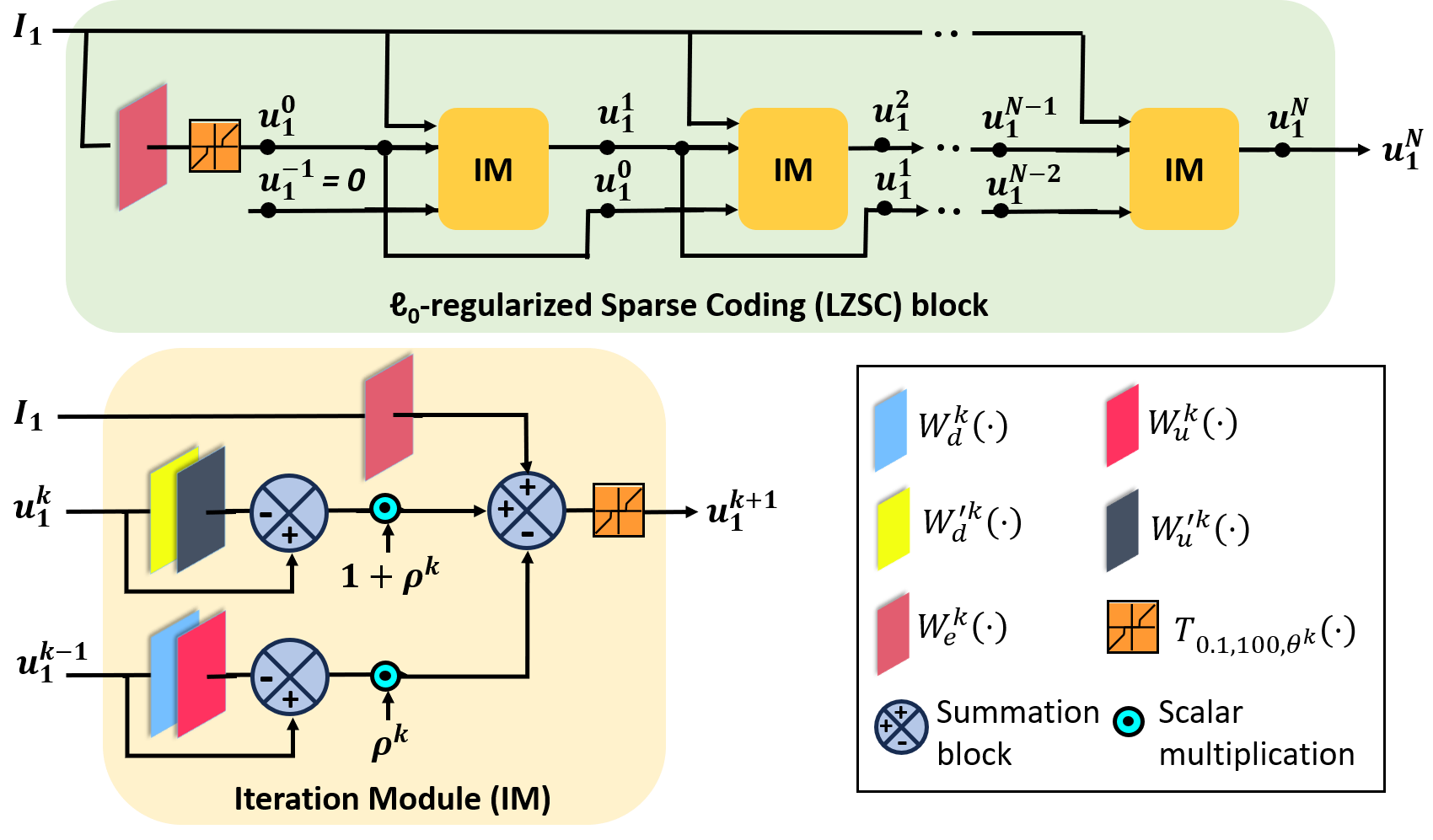
Figure 2: Architecture of proposed LZSC block and the structure of iteration module (IM). Given the input image $I_{1}$, the LZSC block estimates the $\ell_{0}$-regularized sparse feature $u_{1}^{N}$ at $N^{th}$ iteration. The structure of the LZSC block for estimating the sparse features $c$, $u_{2}$, $x_{1}$, and $x_{2}$ is the same; only the input image is different.

III-B Solving the $\ell_{0}$-regularized CSC problem

We consider the $\ell_{0}$ regularized CSC problem for the updation of $u_{1}$ (Eqn. 9),

$$\underset{u_{1}}{\mathrm{Argmin}}\>\frac{1}{2}\Big{|}\Big{|}\>I_{1}-D_{u}(u_{1})\Big{|}\Big{|}_{2}^{2}+\lambda_{u_{1}}||u_{1}||_{0}$$

To solve this, inspired by [16], we first propose a convolutional extension of the NIHTA iteration step in Eqn 2. Thus, the iteration step for updating $u_{1}$ becomes,

$$u_{1}^{k+1}=H_{\theta}\Big{(}u_{1}^{k}-W_{u}\Big{(}W_{d}\Big{(}u_{1}^{k}\Big{)}-I_{1}\Big{)}\Big{)}$$ (15)

where $u_{1}^{k}$ is the sparse estimation at $k^{th}$ iteration, $W_{u}(\cdot)$ and $W_{d}(\cdot)$ are learnable convolution layers, and $\theta$ is a learnable parameter. However, in Eqn. 15, the current estimation $u_{1}^{k+1}$ only depends on the previous estimation $u_{1}^{k}$. To improve the convergence, we can introduce Neterov’s momentum [25] which considers the previous two estimation steps $u_{1}^{k}$ and $u_{1}^{k-1}$ to update the current estimation. Inspired by [36], we introduce Nesterov’s momentum in Equation 15 to update $u_{1}$ as,

$$\begin{split}u_{1}^{k}&=H_{\theta}\Big{(}v^{k}-W_{u}\Big{(}W_{d}\Big{(}v^{k}\Big{)}\Big{)}+W_{u}\Big{(}I_{1}\Big{)}\Big{)}\\ v^{k+1}&=u_{1}^{k}+\rho^{k}\big{(}u_{1}^{k}-u_{1}^{k-1}\big{)}\end{split}$$ (16)

where $\rho^{k}$, a learnable parameter, is the update weight at each iteration and should increase monotonously with iteration number $k$. Now combining the two steps in Eqn. 16, we get,

$$\begin{split}u_{1}^{k+1}=H_{\theta}\Big{(}&\Big{(}1+\rho^{k}\Big{)}\Big{(}u_{1}^{k}-W_{u}\Big{(}W_{d}\Big{(}u_{1}^{k}\Big{)}\Big{)}\Big{)}\\ &-\rho^{k}\Big{(}u_{1}^{k-1}-W_{u}\Big{(}W_{d}\Big{(}u_{1}^{k-1}\Big{)}\Big{)}\Big{)}\\ &+W_{u}\Big{(}I_{1}\Big{)}\Big{)}\end{split}$$ (17)

In Eqn. 17, the convolutional layers are the same for all the iterations. However, having different learnable layers and parameters at each iteration usually improves the performance [20]. Moreover, the estimation accuracy improves if we have different convolutional layers for the input $I_{1}$ [37]. Motivated by these, we update the iteration step as,

$$\begin{split}u_{1}^{k+1}=H_{\theta^{k}}\Big{(}&\Big{(}1+\rho^{k}\Big{)}\Big{(}u_{1}^{k}-W_{u}^{k}\Big{(}W_{d}^{k}\Big{(}u_{1}^{k}\Big{)}\Big{)}\Big{)}\\ &-\rho^{k}\Big{(}u_{1}^{k-1}-W_{u}^{k}\Big{(}W_{d}^{k}\Big{(}u_{1}^{k-1}\Big{)}\Big{)}\Big{)}\\ &+W_{e}^{k}\Big{(}I_{1}\Big{)}\Big{)}\end{split}$$ (18)

$W_{u}^{k}(\cdot)$, $W_{d}^{k}(\cdot)$ and $W_{e}^{k}(\cdot)$ are learnable convolution layers at each iteration. Moreover, we propose to use different convolution layers for $u_{1}^{k}$ and $u_{1}^{k-1}$ for better learning,

$$\begin{split}u_{1}^{k+1}=H_{\theta^{k}}\Big{(}&\Big{(}1+\rho^{k}\Big{)}\Big{(}u_{1}^{k}-W_{u}^{k}\Big{(}W_{d}^{k}\Big{(}u_{1}^{k}\Big{)}\Big{)}\Big{)}\\ &-\rho^{k}\Big{(}u_{1}^{k-1}-W_{u}^{{}^{\prime}k}\Big{(}W_{d}^{{}^{\prime}k}\Big{(}u_{1}^{k-1}\Big{)}\Big{)}\Big{)}\\ &+W_{e}^{k}\Big{(}I_{1}\Big{)}\Big{)}\end{split}$$ (19)

$W_{u}^{{}^{\prime}k}(\cdot)$ and $W_{d}^{{}^{\prime}k}(\cdot)$ are learnable convolution layers at each iteration. As discussed in Section II-A, we replace the discontinuous thresholding function $H_{\theta^{k}(\cdot)}$ with a continuous function $T_{0.1,100,\theta^{k}}(\cdot)$ for better network training. Finally, the iteration step for updating $u_{1}$ becomes,

$$\begin{split}u_{1}^{k+1}=T_{0.1,100,\theta^{k}}\Big{(}&\Big{(}1+\rho^{k}\Big{)}\Big{(}u_{1}^{k}-W_{u}^{k}\Big{(}W_{d}^{k}\Big{(}u_{1}^{k}\Big{)}\Big{)}\Big{)}\\ &-\rho^{k}\Big{(}u_{1}^{k-1}-W_{u}^{{}^{\prime}k}\Big{(}W_{d}^{{}^{\prime}k}\Big{(}u_{1}^{k-1}\Big{)}\Big{)}\Big{)}\\ &+W_{e}^{k}\Big{(}I_{1}\Big{)}\Big{)}\end{split}$$ (20)

In Eqn. 20, $\theta^{k}$ and $\rho^{k}$ are learnable, and they may learn non-positive values, which contradicts their definition. Moreover, $\rho^{k}$ should be within $0$ to $1$ and increase with the iteration number $k$ for better convergence. Also, $\theta^{k}$ should decrease with the iteration number $k$ as the sparse estimation accuracy improves with $k$. Inspired by [38], we constrain $\theta^{k}$ and $\rho^{k}$ as,

$$\begin{split}&\theta^{k}=sp(w_{\theta}k+b_{\theta})\>\>,\>\>w_{\theta}<0\\ &\rho^{k}=\frac{sp(w_{\rho}k+b_{\rho})-sp(b_{\rho})}{sp(w_{\rho}k+b_{\rho})}\>\>,\>\>w_{\rho}<0\end{split}$$ (21)

$sp(\cdot)$ denotes the softplus function. Here, $w_{\theta}$, $b_{\theta}$, $w_{\rho}$ and $b_{\rho}$ are the parameters which are learned.

By unfolding the iteration steps in Eqn. 20, we design the iteration module (IM) shown in Fig. 2. Moreover, we assume $u_{1}^{k}=0;\>\>\forall k<0$, and stack multiple IMs to construct the LZSC block. We utilize this LZSC block to design our fusion network FNet and inverse fusion network IFNet, the details of which are described in the next subsection.

III-C Network Architectures

The proposed FNet architecture is illustrated in Fig. 3. Given the source images $I_{1}$ and $I_{2}$ from different modalities, first the unique features $u_{1}$ and $u_{2}$ are estimated using two LZSC blocks. Then we get $\hat{I}_{1}$ and $\hat{I}_{2}$ as,

$$\hat{I}_{1}=I_{1}-D_{u_{1}}(u_{1}),\>\>\hat{I}_{2}=I_{2}-D_{u_{2}}(u_{2})$$ (22)

Following this, $\hat{I}_{1}$ and $\hat{I}_{2}$ are channel-wise concatenated to get $\hat{I}_{1,2}$. Then, the common feature $c$ is estimated from $\hat{I}_{1,2}$ using one LZSC block. Finally, we generate the fused image $I_{f}$ from the unique and common features as,

$$I_{f}=G_{c}(c)+G_{u_{1}}(u_{1})+G_{u_{2}}(u_{2})$$ (23)

The proposed IFNet architecture is also illustrated in Fig. 4. Given the fused image $I_{f}$, first, we estimate $x_{1}$ and $x_{2}$, the features corresponding to $I_{1}$ and $I_{2}$ using two LZSC blocks. Then, $I_{1}$ and $I_{2}$ are obtained by,

$$I_{1}=D_{x_{1}}(x_{1}),\>\>I_{2}=D_{x_{2}}(x_{2})$$ (24)

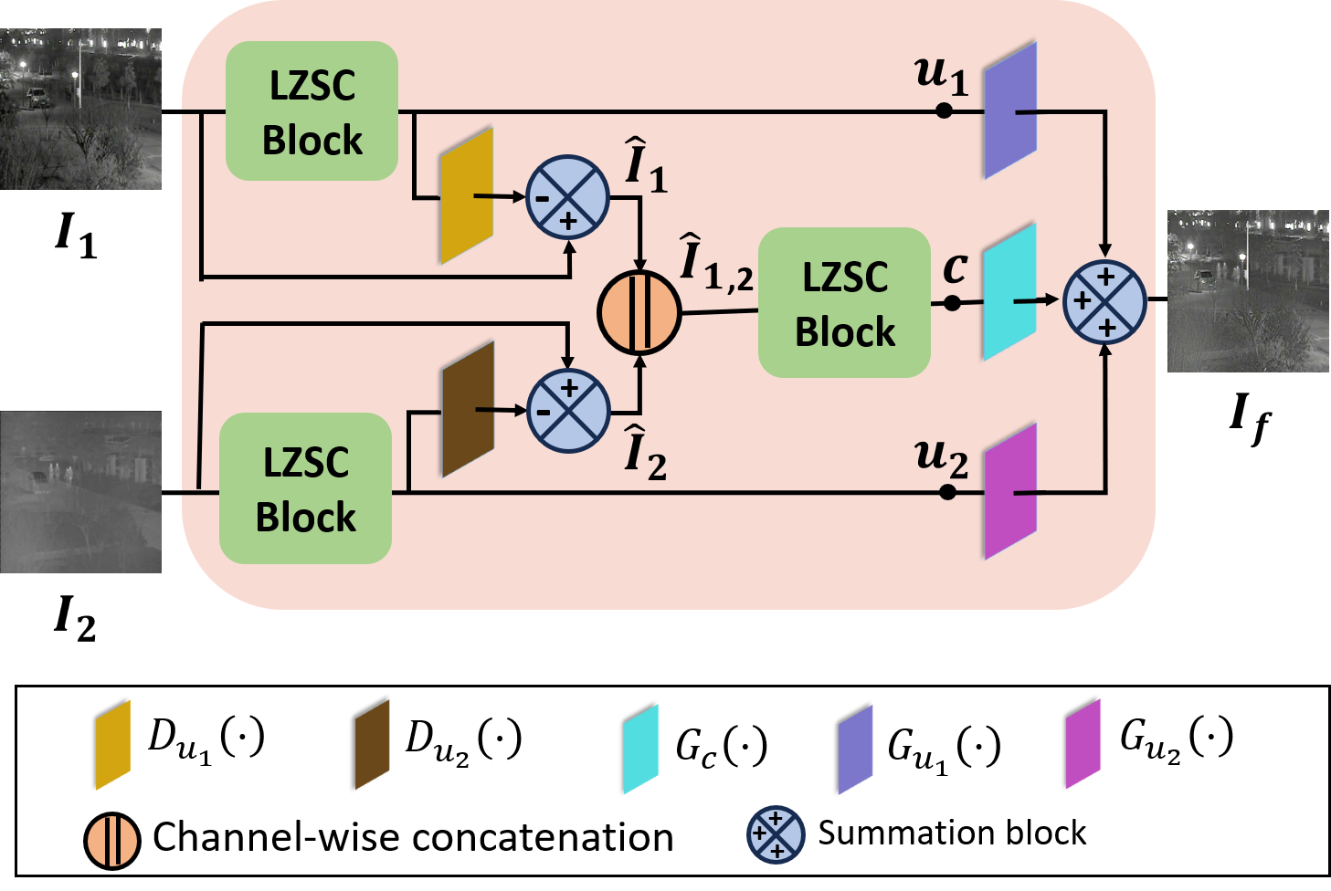
Figure 3: Architecture of proposed FNet. Given the source images $I_{1}$ and $I_{2}$, FNet generates the fused image $I_{f}$.

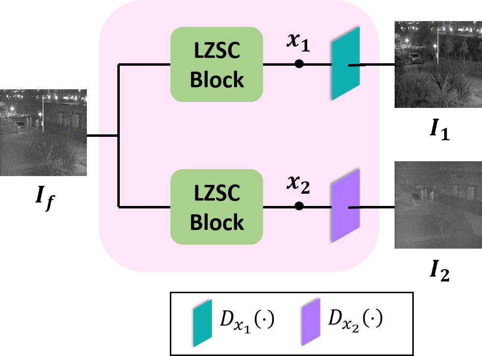
Figure 4: Architecture of proposed IFNet. Given the fused image $I_{f}$, IFNet generates the source images $I_{1}$ and $I_{2}$.

TABLE I: Performance comparison for VIS-IR, VIS-NIR, CT-MRI, PET-MRI, and SPECT-MRI image fusion tasks. The FLOPs and runtime values are reported under the setting of fusing two source images of resolution $320\times 320$. We highlight the best and second-best performances in red and blue colors respectively. $\uparrow$ means high value desired.

III-D Training Process

In the MMIF task, where the ground truth fused image is not available, a two-stage training procedure can be very effective [31]. Motivated by this, we propose a two-stage training procedure for FNet. Fig. 5 shows the two-stage training pipeline. The details are described below.

Training stage I. We consider both the fusion and inverse fusion processes in the training stage I. The idea is that the original source images should be the same as the source images generated in the inverse fusion process. Given the source images $I_{1}$ and $I_{2}$, we generate the fused image $I_{f}$ using FNet. Then, $I_{f}$ is input to IFNet to generate the source images $I_{1}^{{}^{\prime}}$ and $I_{2}^{{}^{\prime}}$. The training constraints $I_{1}^{{}^{\prime}}$ to be similar to $I_{1}$ and $I_{2}^{{}^{\prime}}$ to be similar to $I_{2}$, using the loss function,

$$\mathcal{L}^{I}=\mathcal{L}(I_{1}^{{}^{\prime}},I_{1})+\mathcal{L}(I_{2}^{{}^{\prime}},I_{2})$$ (25)

where, $\mathcal{L}(I_{1}^{{}^{\prime}},I_{1})=||\>I_{1}^{{}^{\prime}}-I_{1}\>||_{1}+||\>\nabla I_{1}^{{}^{\prime}}-\nabla I_{1}\>||_{1}$. $\nabla$ is the Sobel gradient operator. Both FNet and IFNet are trained in the training stage I.

Training stage II. We consider only the fusion process in the training stage II. Our motivation is to constrain the generated fused image to have maximum similarity with the source images. Here, the source images $I_{1}$ and $I_{2}$ are fed to a nearly well-trained FNet to generate $I_{f}$. Inspired by [1], the total loss is.

$$\mathcal{L}^{II}=\beta_{1}\mathcal{L}_{int}+\beta_{2}\mathcal{L}_{grad}+\beta_{3}\mathcal{L}_{ssim}$$ (26)

where $\mathcal{L}_{int}=||\>I_{f}-max(I_{1},I_{2})\>||_{1}$, $\mathcal{L}_{grad}=||\>\nabla I_{f}-max(\nabla I_{1},\nabla I_{2})\>||_{1}$. $\mathcal{L}_{ssim}=w_{1}(1-ssim(I_{1},I_{f}))+w_{2}(1-ssim(I_{2},I_{f}))$. $ssim(\cdot)$ is the structural similarity index measure between two images. $w_{1}=\frac{\nabla I_{1}}{\nabla I_{1}+\nabla I_{2}}$, $w_{2}=\frac{\nabla I_{2}}{\nabla I_{1}+\nabla I_{2}}$. $\beta_{1}$, $\beta_{2}$ and $\beta_{3}$ are tuning parameters.

IV Experiments

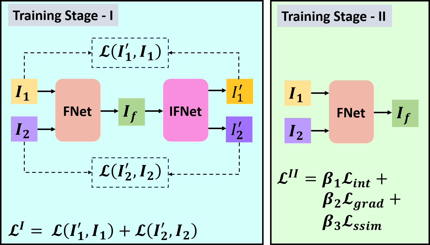
Figure 5: Pipeline for two-stage training of our proposed FNet.

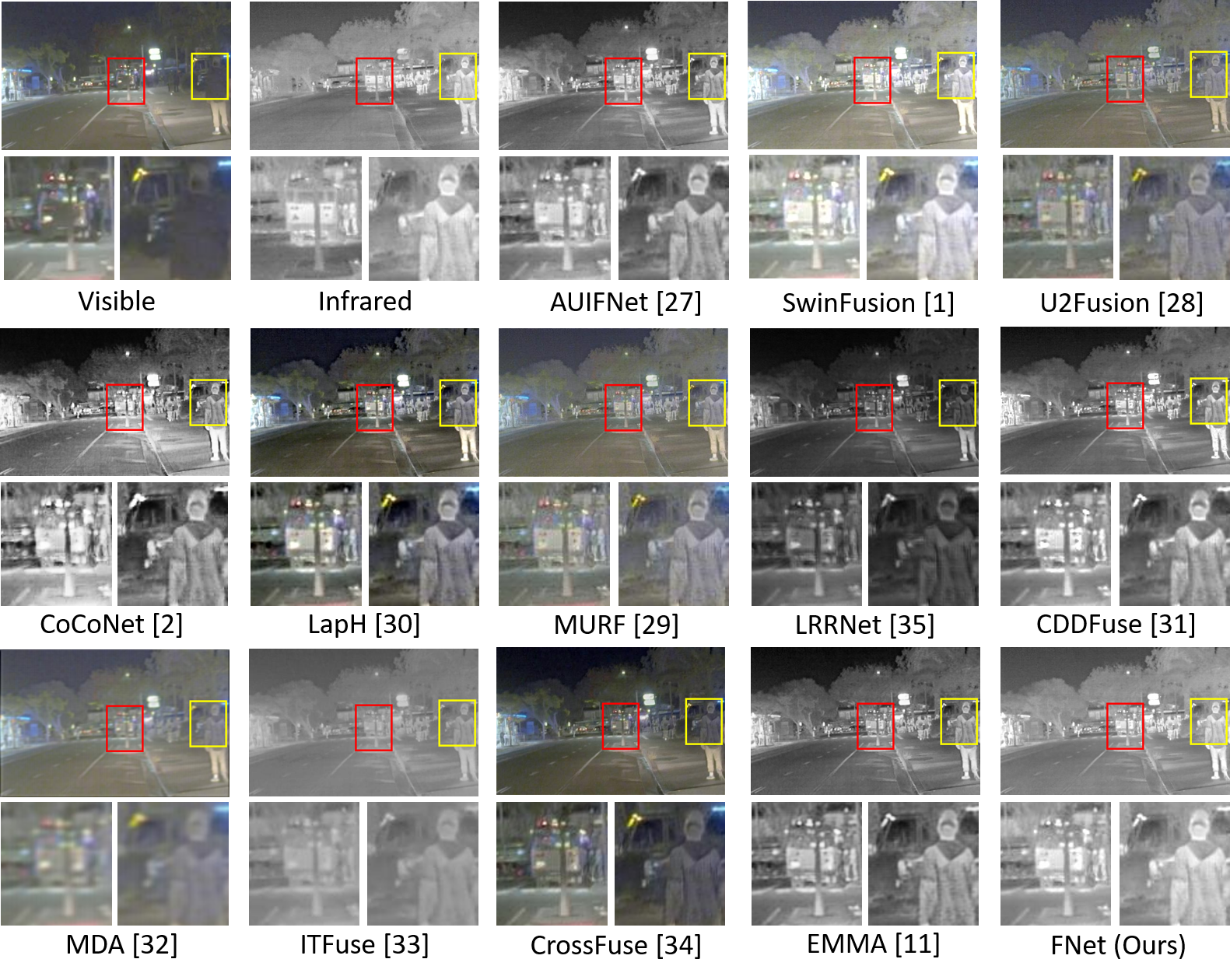
Figure 6: Visual comparison with the SOTA methods for the VIS-IR image fusion task on the RoadScene dataset. Compared to SwinFusion [1] and CDDFuse [31], our proposed FNet better preserves the structure information of the source images.

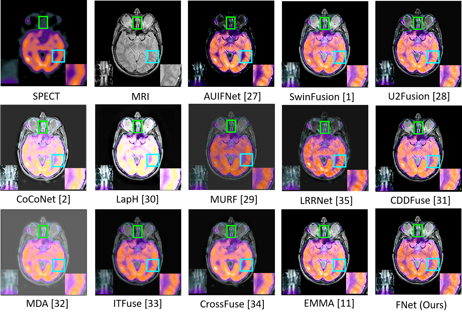
Figure 7: Visual comparison with the SOTA methods for the MRI-SPECT image fusion task on Harvard medical dataset. Compared to SwinFusion [1] and CDDFuse [31], our FNet better preserves the structure information of the source images.

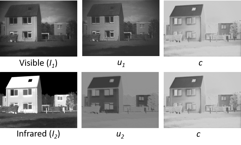
Figure 8: Visualization of estimated unique and common features for the VIS-IR image fusion task on TNO dataset.

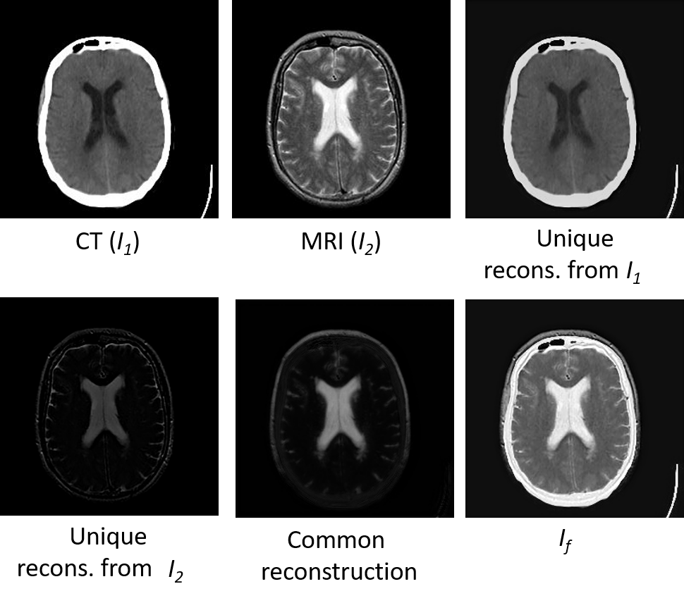
Figure 9: Visualization of unique and common reconstruction for the CT-MRI fusion task on Harvard medical dataset.

The performance of our proposed FNet is evaluated on five MMIF tasks: i) VIS-IR, ii) VIS-NIR, iii) CT-MRI, iv) PET-MRI, and v) SPECT-MRI image fusion. Section IV-A presents the experimental setup, including implementation details, datasets, training settings, and evaluation metrics. Then, we report the quantitative and qualitative comparison results with the SOTA methods in Section IV-B. The intermediate features are visualized in Section IV-C to show the good network interpretability of our FNet. In Section IV-D, we compare FNet with SOTA methods on downstream object detection in VIS-IR image pairs. Finally, in Section IV-E, ablation experiments are conducted to demonstrate the effectiveness of our proposed method.

IV-A Experimental Setup

Implementation details. In FNet, each convolution layer is set to have kernel size $9\times 9$, and number of filters $K=64$. In the LZSC block, the number of IMs is set to $4$. We set the tuning parameters $\beta_{1}=20,\beta_{2}=20,\beta_{3}=15$ for the loss function in Eqn. 26.

Datasets. For both training and testing, publicly available datasets are used. We train FNet with $1,444$ image pairs from the MSRS VIS-IR dataset [1] and test on other datasets without any fine-tuning to check the model’s generalization ability. We test: i) VIS-IR task on $20$ image pairs from the TNO dataset [39], and $50$ image pairs from the RoadScene dataset [28], ii) VIS-NIR task on $20$ image pairs from the RGB-NIR Scene dataset [40], iii) CT-MRI task on $21$ image pairs from the Harvard medical dataset [41], iv) PET-MRI task on $42$ image pairs from the Harvard medical dataset and v) SPECT-MRI task on $73$ image pairs from the Harvard medical dataset.

Training settings. We train FNet in two stages. In both stages, the training is conducted with Adam optimizer with a constant learning rate of $1\times 10^{-4}$ for $20,000$ iterations with a batch size of $16$. In each iteration, we randomly crop the image pairs to patch size $128\times 128$ and augment them by horizontal and vertical flipping. All experiments are conducted using NVIDIA A40 GPU within the PyTorch framework.

Evaluation metrics. We objectively compare fusion performance with four metrics: mutual information (MI), visual information fidelity (VIF) [42], edge information (Qabf) [43], and structural similarity index measure (SSIM) [44]. A higher value of MI, VIF, Qabf, and SSIM indicates superior fusion performance. We follow the calculation given in [31].

IV-B Performance Comparison with the SOTA Methods

FNet is compared with twelve recent SOTA methods: AUIFNet [27], SwinFusion [1], U2Fusion [28], CoCoNet [2], LapH [30], MURF [29], LRRNet [35], CDDFuse [31], MDA [32], ITFuse [33], CrossFuse [34], and EMMA [11].

IV-B1 Quantitative Comparison

Table I shows the quantitative comparison for MMIF tasks on six datasets. Along with the MI, VIF, Qabf, and SSIM metrics, we also list the model parameters, FLOPs, and average GPU runtime. FLOPs and average runtime values are reported under the setting of fusing two source images of resolution $320\times 320$. FNet has the leading performance on almost all four metrics across the six datasets. The results demonstrate that FNet can preserve the essential structural information of the source images. Among the other SOTA methods, SwinFusion and CDDFuse have comparable performance with our method. It is worth noting that FNet has much lower parameters, FLOPs, and runtime than these two methods.

IV-B2 Qualitative Comparison

Fig. 6 shows a visual comparison of FNet with the SOTA methods for the VIS-IR image fusion task on the RoadScene dataset. FNet successfully separates the common background in the VIS-IR image pairs, unique scene details in the visible image, and unique objects in the infrared image and combines all this information to generate the fused image. Compared to the SOTA methods, FNet can better preserve the structure and texture details of the source images in the fused image.

Fig. 7 shows a visual comparison of the SPECT-MRI image fusion task on the Harvard medical dataset. Our FNet effectively separates the common edge details in the SPECT-MRI image pairs, the unique functional details in the SPECT image, and the tissue details in the MRI image and combines all these features into the fused image. Compared to the SOTA methods, FNet can better preserve the tissue and structure details of the source images. More visual comparison results are given in the supplementary material.

TABLE II: mAP@[0.5:0.95] values for object detection on the M3FD dataset. We highlight the best and second-best performances in red and blue colors respectively. A high value of mAP@[0.5:0.95] is desired.

TABLE III: Comparison results of ablation experiments. Highlighted results are the best ones.

IV-C Visualization of Intermediate Results

IV-C1 Visualization of unique and common features

In our MMIF network FNet, we use three LZSC blocks to estimate the unique and common features from the different modality source images. This provides interpretability of the underlying fusion process. Fig. 8 shows the estimated unique and common features for the VIS-IR image fusion task on the TNO dataset. The unique extraction $u_{1}$ from the visible image ($I_{1}$) consists of the scene details. This information can not be captured by an infrared image ($I_{2}$). The unique extraction $u_{2}$ from the infrared image consists of the details of the thermal radiation, which does not exist in the visible image. Thus, the unique features of visible and infrared images are specific to their own modality. The common feature $c$ extracted from the visible and infrared images is the edges of the different objects.

IV-C2 Visualization of unique and common reconstruction

In FNet, we first estimate the unique and common features. Then these features undergo convolution operations to obtain the unique and common reconstruction parts, which are then added to get the fused image. Fig. 9 shows the unique and common reconstructions of the CT-MRI image fusion task on the Harvard medical dataset. As we can see, the unique reconstruction from the CT image ($I_{1}$) preserves the anatomical information, whereas the unique part of the MRI image ($I_{2}$) has the tissue details. The common reconstruction part consists of the shapes that are present in both the images. The fused image $I_{f}$ consists of the unique and common reconstruction parts. More visualization of intermediate results are given in the supplementary material.

IV-D Performance on Downstream Object Detection

We also study the impact of VIS-IR image fusion on the downstream object detection task. YOLOv5 [45], a SOTA detection network is utilized to assess the object detection performance on source images and fused images. We use the M3FD dataset [46], which has $4200$ pairs of VIS-IR images. The images have objects of six categories: people, cars, trucks, buses, lamps, and motorcycles. For a fair comparison, we input the visible images, infrared images, and fused images generated using different methods into the YOLOv5 detector for training and testing. We utilize $3800$ images for training and $400$ images for testing. For training, SGD optimizer is used for training $100$ epochs. The batch size and initial learning rate are set to $16$ and $1\times 10^{-2}$, respectively. The object detection performance is evaluated using map@[$0.5:0.95$], which denotes the mean average precision values at different IoU thresholds (from $0.5$ to $0.95$ in steps of $0.05$). Table II shows the comparison for object detection performance. Except for MDA, all the fusion methods have better detection performance than the source images. Compared to the SOTA fusion methods, our FNet has superior performance.

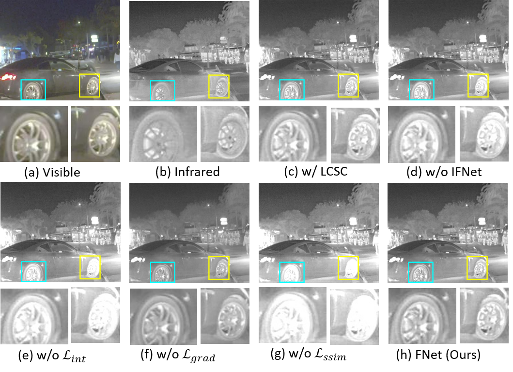
Figure 10: Visual comparison of the ablation experiments for the VIS-IR task on the TNO dataset.

IV-E Ablation Study

Our proposed FNet’s performance relies on the network design and two-stage training procedure. Especially, our proposed LZSC block effectively estimates the $\ell_{0}$-regularized common and sparse features from the source images, which are then combined to get the final fused image. Moreover, we design an inverse fusion network named IFNet, which is utilized in the training stage I of FNet. In the training stage II, we constrain the fused image to be similar to the source images using a three-component loss function. In this section, we conduct the following ablation experiments to validate the effectiveness of our proposed method. The visual comparison results of ablation experiments of the VIS-IR image fusion task on the RoadScene dataset are presented in Fig. 10.

Effectiveness of LZSC block: Our novel LZSC block is designed to estimate the $\ell_{0}$-regularized sparse features from an input image. To validate the effectiveness of the LZSC block in FNet and IFNet, we replace it with the LCSC block [16]. The implementation details of the LCSC block is given in the supplementary material. As depicted in Fig. 10-(c), the model w/ the LCSC block produces a fused image with less texture details.

Effectiveness of IFNet: Our inverse fusion network IFNet is utilized in the training stage-I of FNet. We constrain the source images generated using IFNet to be similar to the original source images, which effectively improves the performance of FNet. To validate the effectiveness of IFNet, we remove the training stage I of FNet. As shown in Fig. 10-(d), w/o IFNet, the model generates blurred fused image. Also, the structure information from source images is not preserved.

Effectiveness of Loss Function: In the training stage-II, we use a loss function consisting of intensity ($\mathcal{L}_{int}$), gradient ($\mathcal{L}_{grad}$) and ssim ($\mathcal{L}_{ssim}$) loss components. As shown in Fig. 10-(e), w/o $\mathcal{L}_{int}$, the model fails to preserve the texture and color intensity information. Fig. 10-(f) shows that w/o $\mathcal{L}_{grad}$, the generated fused images are dark, and the contrast between foreground and background is not maintained. As shown in Fig. 10-(f), w/o $\mathcal{L}_{ssim}$, the model fails to keep the structure information and texture details of the source images.

Table III presents the quantitative comparison of the ablation experiments on five MMIF tasks. As we can see from the results, in all the ablation experiments, the MMIF performance degrades to a lesser or greater extent. All these results show the effectiveness of our method.

V Conclusion

This work introduces an interpretable network named FNet for the MMIF task. We design our network based on a novel $\ell_{0}$-regularized MCSC model, due to which FNet has advantages of both the interpretability of model-based methods and the efficiency of DNN. Specifically, we propose a novel LZSC block to solve the $\ell_{0}$-regularized CSC problem. Using three LZSC blocks, FNet separates the source images into unique and common features, which are then combined to get the final fused image. Moreover, we propose a novel $\ell_{0}$-regularized MCSC model for the inverse fusion process, based on which we design an inverse fusion network named IFNet. Employing IFNet in the training of FNet significantly improves the MMIF performance. Extensive experiments on six datasets for five MMIF tasks demonstrate that FNet has superior performance than the SOTA methods. Besides, FNet also facilitates downstream object detection in VIS-IR image pairs. Moreover, we also provide visualization of the unique and common sparse features and reconstruction parts, which shows good interpretability of our network. Future work could explore more intricate models to represent the dependency of source images across different modalities for the fusion process and, based on these models, design more interpretable networks for the MMIF task.

References

- [1] J. Ma, L. Tang, F. Fan, J. Huang, X. Mei, and Y. Ma, “SwinFusion: Cross-domain long-range learning for general image fusion via swin transformer,” IEEE/CAA Journal of Automatica Sinica, vol. 9, no. 7, pp. 1200–1217, 2022.
- [2] J. Liu, R. Lin, G. Wu, R. Liu, Z. Luo, and X. Fan, “CoCoNet: Coupled contrastive learning network with multi-level feature ensemble for multi-modality image fusion,” International Journal of Computer Vision, pp. 1–28, 2023.
- [3] F. G. Veshki, N. Ouzir, S. A. Vorobyov, and E. Ollila, “Coupled feature learning for multimodal medical image fusion,” arXiv preprint arXiv:2102.08641, 2021. [Online]. Available: https://arxiv.org/pdf/2102.08641
- [4] X. Deng and P. Dragotti, “Deep convolutional neural network for multi-modal image restoration and fusion,” IEEE Transactions on Pattern Analysis and Machine Intelligence, vol. 43, no. 10, pp. 3333–3348, oct 2021.
- [5] F. G. Veshki and S. A. Vorobyov, “Coupled feature learning via structured convolutional sparse coding for multimodal image fusion,” in ICASSP 2022-2022 IEEE International Conference on Acoustics, Speech and Signal Processing (ICASSP). IEEE, 2022, pp. 2500–2504.
- [6] S. Boyd, N. Parikh, E. Chu, B. Peleato, J. Eckstein et al., “Distributed optimization and statistical learning via the alternating direction method of multipliers,” Foundations and Trends® in Machine learning, vol. 3, no. 1, pp. 1–122, 2011.
- [7] I. Daubechies, M. Defrise, and C. De Mol, “An iterative thresholding algorithm for linear inverse problems with a sparsity constraint,” Communications on Pure and Applied Mathematics: A Journal Issued by the Courant Institute of Mathematical Sciences, vol. 57, no. 11, pp. 1413–1457, 2004.
- [8] K. Wu, Y. Guo, Z. Li, and C. Zhang, “Sparse coding with gated learned ista,” in International conference on learning representations, 2020.
- [9] V. Papyan, Y. Romano, and M. Elad, “Convolutional neural networks analyzed via convolutional sparse coding,” Journal of Machine Learning Research, vol. 18, no. 83, pp. 1–52, 2017.
- [10] H. Zhang and J. Ma, “SDNet: A versatile squeeze-and-decomposition network for real-time image fusion,” International Journal of Computer Vision, pp. 1–25, 2021.
- [11] Z. Zhao, H. Bai, J. Zhang, Y. Zhang, K. Zhang, S. Xu, D. Chen, R. Timofte, and L. Van Gool, “Equivariant multi-modality image fusion,” in Proceedings of the IEEE/CVF Conference on Computer Vision and Pattern Recognition, 2024, pp. 25 912–25 921.
- [12] V. Monga, Y. Li, and Y. C. Eldar, “Algorithm unrolling: Interpretable, efficient deep learning for signal and image processing,” IEEE Signal Processing Magazine, vol. 38, no. 2, pp. 18–44, 2021.
- [13] M. Elad and M. Aharon, “Image denoising via sparse and redundant representations over learned dictionaries,” IEEE Transactions on Image processing, vol. 15, no. 12, pp. 3736–3745, 2006.
- [14] S. Yang, M. Wang, Y. Chen, and Y. Sun, “Single-image super-resolution reconstruction via learned geometric dictionaries and clustered sparse coding,” IEEE Transactions on Image Processing, vol. 21, no. 9, pp. 4016–4028, 2012.
- [15] B. K. Natarajan, “Sparse approximate solutions to linear systems,” SIAM journal on computing, vol. 24, no. 2, pp. 227–234, 1995.
- [16] H. Sreter and R. Giryes, “Learned convolutional sparse coding,” in IEEE International Conference on Acoustics, Speech and Signal Processing (ICASSP), 2018, pp. 2191–2195.
- [17] D. L. Donoho and M. Elad, “Optimally sparse representation in general (nonorthogonal) dictionaries via minimization,” Proceedings of the National Academy of Sciences, vol. 100, no. 5, pp. 2197–2202, 2003.
- [18] T. Blumensath and M. E. Davies, “Iterative hard thresholding for compressed sensing,” Applied and computational harmonic analysis, vol. 27, no. 3, pp. 265–274, 2009.
- [19] ——, “Normalized iterative hard thresholding: Guaranteed stability and performance,” IEEE Journal of selected topics in signal processing, vol. 4, no. 2, pp. 298–309, 2010.
- [20] B. Xin, Y. Wang, W. Gao, D. Wipf, and B. Wang, “Maximal sparsity with deep networks?” Advances in Neural Information Processing Systems, vol. 29, 2016.
- [21] Z. Wang, Q. Ling, and T. Huang, “Learning deep encoders,” in Proceedings of the AAAI Conference on Artificial Intelligence, vol. 30, no. 1, 2016.
- [22] F. Heide, W. Heidrich, and G. Wetzstein, “Fast and flexible convolutional sparse coding,” in Proceedings of the IEEE Conference on Computer Vision and Pattern Recognition, 2015, pp. 5135–5143.
- [23] V. Papyan, Y. Romano, J. Sulam, and M. Elad, “Convolutional dictionary learning via local processing,” in Proceedings of the IEEE International Conference on Computer Vision, 2017, pp. 5296–5304.
- [24] P. Rodríguez, “Fast convolutional sparse coding with penalty,” in 2018 IEEE XXV International Conference on Electronics, Electrical Engineering and Computing (INTERCON). IEEE, 2018, pp. 1–4.
- [25] Y. Nesterov, “A method for unconstrained convex minimization problem with the rate of convergence ,” in Dokl. Akad. Nauk. SSSR, vol. 269, no. 3, 1983, p. 543.
- [26] C. J. Rozell, D. H. Johnson, R. G. Baraniuk, and B. A. Olshausen, “Sparse coding via thresholding and local competition in neural circuits,” Neural computation, vol. 20, no. 10, pp. 2526–2563, 2008.
- [27] Z. Zhao, S. Xu, J. Zhang, C. Liang, C. Zhang, and J. Liu, “Efficient and model-based infrared and visible image fusion via algorithm unrolling,” IEEE Transactions on Circuits and Systems for Video Technology, pp. 1–1, 2021.
- [28] H. Xu, J. Ma, J. Jiang, X. Guo, and H. Ling, “U2Fusion: A unified unsupervised image fusion network,” IEEE Transactions on Pattern Analysis and Machine Intelligence, 2020.
- [29] H. Xu, J. Yuan, and J. Ma, “MURF: Mutually reinforcing multi-modal image registration and fusion,” IEEE transactions on pattern analysis and machine intelligence, 2023.
- [30] X. Luo, G. Fu, J. Yang, Y. Cao, and Y. Cao, “Multi-modal image fusion via deep laplacian pyramid hybrid network,” IEEE Transactions on Circuits and Systems for Video Technology, vol. 33, no. 12, pp. 7354–7369, 2023.
- [31] Z. Zhao, H. Bai, J. Zhang, Y. Zhang, S. Xu, Z. Lin, R. Timofte, and L. Van Gool, “CDDFuse: Correlation-driven dual-branch feature decomposition for multi-modality image fusion,” in Proceedings of the IEEE/CVF conference on computer vision and pattern recognition, 2023, pp. 5906–5916.
- [32] G. Yang, J. Li, H. Lei, and X. Gao, “A multi-scale information integration framework for infrared and visible image fusion,” Neurocomputing, vol. 600, p. 128116, 2024.
- [33] W. Tang, F. He, and Y. Liu, “ITFuse: An interactive transformer for infrared and visible image fusion,” Pattern Recognition, vol. 156, p. 110822, 2024.
- [34] H. Li and X.-J. Wu, “CrossFuse: A novel cross attention mechanism based infrared and visible image fusion approach,” Information Fusion, vol. 103, p. 102147, 2024.
- [35] H. Li, T. Xu, X.-J. Wu, J. Lu, and J. Kittler, “LRRNet: A novel representation learning guided fusion framework for infrared and visible images,” IEEE Transactions on Pattern Analysis and Machine Intelligence, vol. 45, no. 9, pp. 11 040–11 052, 2023.
- [36] A. Beck and M. Teboulle, “A fast iterative shrinkage-thresholding algorithm for linear inverse problems,” SIAM journal on imaging sciences, vol. 2, no. 1, pp. 183–202, 2009.
- [37] A. Aberdam, A. Golts, and M. Elad, “Ada-lista: Learned solvers adaptive to varying models,” IEEE Transactions on Pattern Analysis and Machine Intelligence, vol. 44, no. 12, pp. 9222–9235, 2022.
- [38] J. Xiang, Y. Dong, and Y. Yang, “FISTA-Net: Learning a fast iterative shrinkage thresholding network for inverse problems in imaging,” IEEE Transactions on Medical Imaging, vol. 40, no. 5, pp. 1329–1339, 2021.
- [39] A. Toet, “The TNO multiband image data collection,” Data in brief, vol. 15, pp. 249–251, 2017.
- [40] M. Brown and S. Süsstrunk, “Multi-spectral SIFT for scene category recognition,” in CVPR 2011. IEEE, 2011, pp. 177–184.
- [41] D. Summers, “Harvard Whole Brain Atlas: www. med. harvard. edu/aanlib/home. html,” Journal of Neurology, Neurosurgery & Psychiatry, vol. 74, no. 3, pp. 288–288, 2003.
- [42] Y. Han, Y. Cai, Y. Cao, and X. Xu, “A new image fusion performance metric based on visual information fidelity,” Information fusion, vol. 14, no. 2, pp. 127–135, 2013.
- [43] C. S. Xydeas, V. Petrovic et al., “Objective image fusion performance measure,” Electronics letters, vol. 36, no. 4, pp. 308–309, 2000.
- [44] Z. Wang, A. C. Bovik, H. R. Sheikh, and E. P. Simoncelli, “Image quality assessment: from error visibility to structural similarity,” IEEE transactions on image processing, vol. 13, no. 4, pp. 600–612, 2004.
- [45] J. Redmon, S. Divvala, R. Girshick, and A. Farhadi, “You only look once: Unified, real-time object detection,” in Proceedings of the IEEE conference on computer vision and pattern recognition, 2016, pp. 779–788.
- [46] J. Liu, X. Fan, Z. Huang, G. Wu, R. Liu, W. Zhong, and Z. Luo, “Target-aware dual adversarial learning and a multi-scenario multi-modality benchmark to fuse infrared and visible for object detection,” in Proceedings of the IEEE/CVF conference on computer vision and pattern recognition, 2022, pp. 5802–5811.