ADMM for 0/1 D-Opt and MESP relaxations

Abstract

The 0/1 D-optimality problem and the Maximum-Entropy Sampling problem are two well-known NP-hard discrete maximization problems in experimental design. Algorithms for exact optimization (of moderate-sized instances) are based on branch-and-bound. The best upper-bounding methods are based on convex relaxation. We present ADMM (Alternating Direction Method of Multipliers) algorithms for solving these relaxations and experimentally demonstrate their practical value.

1 Introduction

We assume some familiarity with convex optimization, see [BV04] for example, and with ADMM (Alternating Direction Method of Multipliers) in particular, see [BPC⁺11] for example.

When we can implement the iteration updates quickly, ADMM (and other first-order methods), are a method of choice for approximately solving large-scale convex-optimization problems. A key application can be in the general area of convex MINLO (mixed-integer nonlinear optimization), where the work-horse algorithm is B&B (branch-and-bound), and many convex relaxations must be solved very quickly (see, for example [BBC⁺08]).

Nice families of convex integer nonlinear-optimization problems come from the area of experimental design. One key problem is the Gaussian case of the 0/1 D-optimality problem (D-Opt). Briefly, the problem aims to select a subset of $s$ design points, from a universe of $n$ given design points in $\mathbb{R}^{m}$, with the goal of minimizing the “generalized variance” of the least-squares parameter estimates; see, for example, [PFL23] and the references therein. Another problem is the Gaussian case of the maximum-entropy sampling problem (MESP). Here we have an input covariance matrix of order $n$, and we wish to select a principal submatrix of order $s$, so as to maximize the “differential entropy” (see, for example, [FL22]). In what follows, we present fast ADMM algorithms to solve convex relaxations for 0/1 D-Opt and MESP.

Literature review. D-optimality, whose criterion is maximizing $\operatorname{ldet}$ of an appropriate positive-definite matrix, is a very well-studied topic in the experimental design literature. There are many variations, and we concentrate on the 0/1 version of the problem, which we carefully state in §2. A recent reference on the state-of-the-art for B&B approaches is [PFL23], with many references therein to background and previous work. A key upper bound based on convex relaxation is the “natural bound”, and we propose herein an ADMM algorithm for its fast calculation. Related to this is [NNN⁺21], which proposes an ADMM for “A-optimal design” (which seeks to maximize a trace). More similar is [SMG10], which gives an ADMM algorithm for $\max\{\operatorname{ldet}(X)-\operatorname{Tr}(SX)-\tau\|X\|_{1}\}$, a convex relaxation for “sparse inverse covariance selection”.

MESP is a closely related problem in the experimental design literature, which we carefully state in §3. A recent reference on the state-of-the-art for B&B approaches is [FL22], with many references therein to background and previous work. Key upper bounds based on convex relaxation are the “linx bound” (see [Ans20]) and the “factorization bound” (see [Nik15, LX23, FL22, CFL23]), and we propose herein new ADMM algorithms for their calculation. There is also an important “factorization bound” for 0/1 D-optimality instances, but we can see it as applying the MESP “factorization bound” to an appropriately-constructed instance of MESP (see [PFL23]).

Organization and contributions. In §2, we present a new ADMM algorithm for the natural bound for D-Opt. In §3, we present a new ADMM algorithm for the factorization bound for MESP, which requires significant new theoretical results. We also present a new ADMM algorithm for the linx bound for MESP. In §4, we present results of numerical experiments, demonstrating the benefits of our approach. Specifically, we will see that our ADMM algorithm for the natural bound for D-Opt is significantly better than applying commercial solvers. Additionally, we we will see that while our ADMM algorithm for the linx bound for MESP does not perform well compared to commercial solvers, our ADMM algorithm for the factorization bound does perform quite well. It is noteworthy that on our test instances, the factorization bound is much better than the linx bound. We also have an Appendix that includes proofs.

Notation. We denote an all-ones vector by $\mathbf{e}$, an $i$-th standard unit vector by $\mathbf{e}_{i}$ , the identity matrix of order $n$ by $I_{n}$. We let $\mathbb{S}^{n}$ (resp., $\mathbb{S}^{n}_{+}$ , $\mathbb{S}^{n}_{++}$) denote the set of symmetric (resp., positive-semidefinite, positive-definite) matrices of order $n$. We let $\operatorname{\textstyle{Diag}}(x)$ denote the $n\times n$ diagonal matrix with diagonal elements given by the components of $x\in\mathbb{R}^{n}$, and $\operatorname{\textstyle{diag}}(X)$ denote the $n$-dimensional vector with elements given by the diagonal elements of $X\in\mathbb{R}^{n\times n}$. When $X$ is symmetric, we let $\lambda(X)$ denote its non-increasing list of eigenvalues. We let $\operatorname{ldet}$ denote the natural logarithm of the determinant. We let $\operatorname{Tr}$ denote the trace. We denote Frobenius norm by $\|\cdot\|_{F}$ and 2-norm by $\|\cdot\|_{2}$ . For matrix $M$, we denote row $i$ by $M_{i\cdot}$ and column $j$ by $M_{\cdot j}$ . For compatible $M_{1}$ and $M_{2}$, $M_{1}\bullet M_{2}:=\operatorname{Tr}(M_{1}^{\mathchoice{\raisebox{0.0pt}{$\displaystyle\scriptscriptstyle\mathsf{T}$}}{\raisebox{0.0pt}{$\textstyle\scriptscriptstyle\mathsf{T}$}}{\raisebox{0.0pt}{$\scriptstyle\scriptscriptstyle\mathsf{T}$}}{\raisebox{0.0pt}{$\scriptscriptstyle\scriptscriptstyle\mathsf{T}$}}}M_{2})$ is the matrix dot-product. The $\operatorname{\textstyle{vec}}$ operator creates a column vector from a matrix $A$ by stacking the column vectors of $A$.

In the different subsections, in presenting ADMM algorithms, the primal variables $x$ and $Z$ (and the associated iterates $x^{t}$ and $Z^{t}$), the Lagrange multiplier $\Psi$ (and the associated iterates $\Psi^{t}$), and the iterates $Y^{t}$ have similar uses but different meanings. Throughout, $\theta_{\ell}$ denotes the $\ell$-th greatest eigenvector of $\rho Y^{t+1}$, and $\lambda_{\ell}$ denotes the $\ell$-th greatest eigenvector of $Z^{t+1}$.

2 D-Optimality

The 0/1 D-optimality problem is

$$\max\left\{\operatorname{ldet}\textstyle\left(\sum_{\ell\in N}x_{\ell}v_{\ell}v_{\ell}^{\mathchoice{\raisebox{0.0pt}{$\displaystyle\scriptscriptstyle\mathsf{T}$}}{\raisebox{0.0pt}{$\textstyle\scriptscriptstyle\mathsf{T}$}}{\raisebox{0.0pt}{$\scriptstyle\scriptscriptstyle\mathsf{T}$}}{\raisebox{0.0pt}{$\scriptscriptstyle\scriptscriptstyle\mathsf{T}$}}}\right)~{}:~{}\mathbf{e}^{\mathchoice{\raisebox{0.0pt}{$\displaystyle\scriptscriptstyle\mathsf{T}$}}{\raisebox{0.0pt}{$\textstyle\scriptscriptstyle\mathsf{T}$}}{\raisebox{0.0pt}{$\scriptstyle\scriptscriptstyle\mathsf{T}$}}{\raisebox{0.0pt}{$\scriptscriptstyle\scriptscriptstyle\mathsf{T}$}}}x=s,~{}x\in\{0,1\}^{n}\right\},$$ (D-Opt)

where $v_{\ell}\in\mathbb{R}^{m}$, for $\ell\in N:=\{1,\ldots,n\}$, with $s\geq m$. It is very useful to define $A:=(v_{1},v_{2},\dots,v_{n})^{\mathchoice{\raisebox{0.0pt}{$\displaystyle\scriptscriptstyle\mathsf{T}$}}{\raisebox{0.0pt}{$\textstyle\scriptscriptstyle\mathsf{T}$}}{\raisebox{0.0pt}{$\scriptstyle\scriptscriptstyle\mathsf{T}$}}{\raisebox{0.0pt}{$\scriptscriptstyle\scriptscriptstyle\mathsf{T}$}}}$ (which we always assume has full column rank), and so we have $\sum_{\ell\in N}x_{\ell}v_{\ell}v_{\ell}^{\mathchoice{\raisebox{0.0pt}{$\displaystyle\scriptscriptstyle\mathsf{T}$}}{\raisebox{0.0pt}{$\textstyle\scriptscriptstyle\mathsf{T}$}}{\raisebox{0.0pt}{$\scriptstyle\scriptscriptstyle\mathsf{T}$}}{\raisebox{0.0pt}{$\scriptscriptstyle\scriptscriptstyle\mathsf{T}$}}}=A^{\mathchoice{\raisebox{0.0pt}{$\displaystyle\scriptscriptstyle\mathsf{T}$}}{\raisebox{0.0pt}{$\textstyle\scriptscriptstyle\mathsf{T}$}}{\raisebox{0.0pt}{$\scriptstyle\scriptscriptstyle\mathsf{T}$}}{\raisebox{0.0pt}{$\scriptscriptstyle\scriptscriptstyle\mathsf{T}$}}}\operatorname{\textstyle{Diag}}(x)A$. Relative to the 0/1 D-optimality problem, we consider the natural bound

$$\max\left\{\operatorname{ldet}\left(A^{\mathchoice{\raisebox{0.0pt}{$\displaystyle\scriptscriptstyle\mathsf{T}$}}{\raisebox{0.0pt}{$\textstyle\scriptscriptstyle\mathsf{T}$}}{\raisebox{0.0pt}{$\scriptstyle\scriptscriptstyle\mathsf{T}$}}{\raisebox{0.0pt}{$\scriptscriptstyle\scriptscriptstyle\mathsf{T}$}}}\operatorname{\textstyle{Diag}}(x)A\right)~{}:~{}\mathbf{e}^{\mathchoice{\raisebox{0.0pt}{$\displaystyle\scriptscriptstyle\mathsf{T}$}}{\raisebox{0.0pt}{$\textstyle\scriptscriptstyle\mathsf{T}$}}{\raisebox{0.0pt}{$\scriptstyle\scriptscriptstyle\mathsf{T}$}}{\raisebox{0.0pt}{$\scriptscriptstyle\scriptscriptstyle\mathsf{T}$}}}x=s,~{}x\in[0,1]^{n}\right\}; \mathcal{N}$$ ()

see [PFL23], and the references therein. By introducing a variable $Z\in\mathbb{S}^{m}$, we rewrite $\mathcal{N}$ as

$$\min\left\{-\operatorname{ldet}(Z)~{}:~{}-A^{\mathchoice{\raisebox{0.0pt}{$\displaystyle\scriptscriptstyle\mathsf{T}$}}{\raisebox{0.0pt}{$\textstyle\scriptscriptstyle\mathsf{T}$}}{\raisebox{0.0pt}{$\scriptstyle\scriptscriptstyle\mathsf{T}$}}{\raisebox{0.0pt}{$\scriptscriptstyle\scriptscriptstyle\mathsf{T}$}}}\operatorname{\textstyle{Diag}}(x)A+Z=0,~{}\mathbf{e}^{\mathchoice{\raisebox{0.0pt}{$\displaystyle\scriptscriptstyle\mathsf{T}$}}{\raisebox{0.0pt}{$\textstyle\scriptscriptstyle\mathsf{T}$}}{\raisebox{0.0pt}{$\scriptstyle\scriptscriptstyle\mathsf{T}$}}{\raisebox{0.0pt}{$\scriptscriptstyle\scriptscriptstyle\mathsf{T}$}}}x=s,~{}x\in[0,1]^{n}\right\}.$$ (1)

The augmented Lagrangian function associated to (1) is

$$\mathcal{L}_{\rho}(x,Z,\Psi,\delta)\!=$$

$$\quad\!-\operatorname{ldet}(Z)\!+\!\frac{\rho}{2}\!\left\|-A^{\mathchoice{\raisebox{0.0pt}{$\displaystyle\scriptscriptstyle\mathsf{T}$}}{\raisebox{0.0pt}{$\textstyle\scriptscriptstyle\mathsf{T}$}}{\raisebox{0.0pt}{$\scriptstyle\scriptscriptstyle\mathsf{T}$}}{\raisebox{0.0pt}{$\scriptscriptstyle\scriptscriptstyle\mathsf{T}$}}}\operatorname{\textstyle{Diag}}(x)A\!+\!Z\!+\!\Psi\right\|^{2}_{F}\!+\!\frac{\rho}{2}\!\left(-\mathbf{e}^{\mathchoice{\raisebox{0.0pt}{$\displaystyle\scriptscriptstyle\mathsf{T}$}}{\raisebox{0.0pt}{$\textstyle\scriptscriptstyle\mathsf{T}$}}{\raisebox{0.0pt}{$\scriptstyle\scriptscriptstyle\mathsf{T}$}}{\raisebox{0.0pt}{$\scriptscriptstyle\scriptscriptstyle\mathsf{T}$}}}x\!+\!s+\delta\right)^{2}-\frac{\rho}{2}\!\left\|\Psi\right\|_{F}^{2}-\frac{\rho}{2}\delta^{2},$$

where $\rho>0$ is the penalty parameter and $\Psi\in\mathbb{S}^{m}$, $\delta\in\mathbb{R}$ are the scaled Lagrangian multipliers. Similar to the development of [SMG10] for “sparse inverse covariance selection”, we will apply the ADMM algorithm to (1) , by iteratively solving, for $t=0,1,\ldots$,

$$x^{t+1}:=\textstyle\operatorname*{argmin}_{x\in[0,1]^{n}}\mathcal{L}_{\rho}(x,Z^{t},\Psi^{t},\delta^{t}),$$ (2)

$$Z^{t+1}:=\textstyle\operatorname*{argmin}_{Z}~{}\mathcal{L}_{\rho}(x^{t+1},Z,\Psi^{t},\delta^{t}),$$ (3)

$$\textstyle\Psi^{t+1}:=\Psi^{t}-A^{\mathchoice{\raisebox{0.0pt}{$\displaystyle\scriptscriptstyle\mathsf{T}$}}{\raisebox{0.0pt}{$\textstyle\scriptscriptstyle\mathsf{T}$}}{\raisebox{0.0pt}{$\scriptstyle\scriptscriptstyle\mathsf{T}$}}{\raisebox{0.0pt}{$\scriptscriptstyle\scriptscriptstyle\mathsf{T}$}}}\operatorname{\textstyle{Diag}}(x^{t+1})A+Z^{t+1},$$ (4)

$$\textstyle\delta^{t+1}:=\delta^{t}-\mathbf{e}^{\mathchoice{\raisebox{0.0pt}{$\displaystyle\scriptscriptstyle\mathsf{T}$}}{\raisebox{0.0pt}{$\textstyle\scriptscriptstyle\mathsf{T}$}}{\raisebox{0.0pt}{$\scriptstyle\scriptscriptstyle\mathsf{T}$}}{\raisebox{0.0pt}{$\scriptscriptstyle\scriptscriptstyle\mathsf{T}$}}}x^{t+1}+s.$$

Next, we detail how to solve the subproblems above.

2.1 Update $x$

To update $x$, we consider subproblem (2), more specifically,

$$\begin{array}[]{rl}x^{t+1}&=\textstyle\operatorname*{argmin}_{x\in[0,1]^{n}}\left\{\left\|-A^{\mathchoice{\raisebox{0.0pt}{$\displaystyle\scriptscriptstyle\mathsf{T}$}}{\raisebox{0.0pt}{$\textstyle\scriptscriptstyle\mathsf{T}$}}{\raisebox{0.0pt}{$\scriptstyle\scriptscriptstyle\mathsf{T}$}}{\raisebox{0.0pt}{$\scriptscriptstyle\scriptscriptstyle\mathsf{T}$}}}\operatorname{\textstyle{Diag}}(x)A\!+\!Z^{t}\!+\!\Psi^{t}\right\|^{2}_{F}\!+\!\left(-\mathbf{e}^{\mathchoice{\raisebox{0.0pt}{$\displaystyle\scriptscriptstyle\mathsf{T}$}}{\raisebox{0.0pt}{$\textstyle\scriptscriptstyle\mathsf{T}$}}{\raisebox{0.0pt}{$\scriptstyle\scriptscriptstyle\mathsf{T}$}}{\raisebox{0.0pt}{$\scriptscriptstyle\scriptscriptstyle\mathsf{T}$}}}x\!+\!s+\delta^{t}\right)^{2}\right\}\\ &=\textstyle\operatorname*{argmin}_{x\in[0,1]^{n}}\left\{\left\|Hx-d\right\|^{2}_{2}\right\},\end{array}$$

where $d:=\begin{bmatrix}\operatorname{\textstyle{vec}}(Z^{t}+\Psi^{t})\\ s+\delta^{t}\end{bmatrix}$ and $H:=\begin{bmatrix}G\\ \mathbf{e}^{\mathchoice{\raisebox{0.0pt}{$\displaystyle\scriptscriptstyle\mathsf{T}$}}{\raisebox{0.0pt}{$\textstyle\scriptscriptstyle\mathsf{T}$}}{\raisebox{0.0pt}{$\scriptstyle\scriptscriptstyle\mathsf{T}$}}{\raisebox{0.0pt}{$\scriptscriptstyle\scriptscriptstyle\mathsf{T}$}}}\end{bmatrix}$, where $G\in\mathbb{R}^{m^{2}\times n}$ is a matrix defined as $G_{\cdot\ell}=\operatorname{\textstyle{vec}}\left(v_{\ell}v_{\ell}^{\mathchoice{\raisebox{0.0pt}{$\displaystyle\scriptscriptstyle\mathsf{T}$}}{\raisebox{0.0pt}{$\textstyle\scriptscriptstyle\mathsf{T}$}}{\raisebox{0.0pt}{$\scriptstyle\scriptscriptstyle\mathsf{T}$}}{\raisebox{0.0pt}{$\scriptscriptstyle\scriptscriptstyle\mathsf{T}$}}}\right)$, for $\ell\in N$. Then, we have $Gx=\operatorname{\textstyle{vec}}\left(A^{\mathchoice{\raisebox{0.0pt}{$\displaystyle\scriptscriptstyle\mathsf{T}$}}{\raisebox{0.0pt}{$\textstyle\scriptscriptstyle\mathsf{T}$}}{\raisebox{0.0pt}{$\scriptstyle\scriptscriptstyle\mathsf{T}$}}{\raisebox{0.0pt}{$\scriptscriptstyle\scriptscriptstyle\mathsf{T}$}}}\operatorname{\textstyle{Diag}}(x)A\right)$. This is the well-known bounded-variable least-squares (BVLS) problem, and there are a lot of efficient algorithms to solve it, see [SP95], for example.

2.2 Update $Z$

To update $Z$, we consider subproblem (3), more specifically,

$$Z^{t+1}=\textstyle\operatorname*{argmin}_{Z}\left\{\!-\operatorname{ldet}(Z)\!+\!\frac{\rho}{2}\!\left\|Z\!-\!Y^{t+1}\right\|^{2}_{F}\right\},$$ (5)

where $Y^{t+1}:=A^{\mathchoice{\raisebox{0.0pt}{$\displaystyle\scriptscriptstyle\mathsf{T}$}}{\raisebox{0.0pt}{$\textstyle\scriptscriptstyle\mathsf{T}$}}{\raisebox{0.0pt}{$\scriptstyle\scriptscriptstyle\mathsf{T}$}}{\raisebox{0.0pt}{$\scriptscriptstyle\scriptscriptstyle\mathsf{T}$}}}\operatorname{\textstyle{Diag}}(x^{t+1})A\!-\!\Psi^{t}$. Then we update $Z$ following Proposition 1.

Using exactly the same ideas as [SMG10] (see also [BPC⁺11, Sec. 6.5]), we have the following result and corollary.

Proposition 1 (proof in the Appendix)

Given $Y^{t+1}\in\mathbb{S}^{m}$ and a positive scalar $\rho$. Let $\rho Y^{t+1}=:Q\Theta Q^{\mathchoice{\raisebox{0.0pt}{$\displaystyle\scriptscriptstyle\mathsf{T}$}}{\raisebox{0.0pt}{$\textstyle\scriptscriptstyle\mathsf{T}$}}{\raisebox{0.0pt}{$\scriptstyle\scriptscriptstyle\mathsf{T}$}}{\raisebox{0.0pt}{$\scriptscriptstyle\scriptscriptstyle\mathsf{T}$}}}$ be the eigendecomposition, where $\Theta:=\operatorname{\textstyle{Diag}}(\theta_{1},\dots,\theta_{m})$ and $Q^{\mathchoice{\raisebox{0.0pt}{$\displaystyle\scriptscriptstyle\mathsf{T}$}}{\raisebox{0.0pt}{$\textstyle\scriptscriptstyle\mathsf{T}$}}{\raisebox{0.0pt}{$\scriptstyle\scriptscriptstyle\mathsf{T}$}}{\raisebox{0.0pt}{$\scriptscriptstyle\scriptscriptstyle\mathsf{T}$}}}Q=QQ^{\mathchoice{\raisebox{0.0pt}{$\displaystyle\scriptscriptstyle\mathsf{T}$}}{\raisebox{0.0pt}{$\textstyle\scriptscriptstyle\mathsf{T}$}}{\raisebox{0.0pt}{$\scriptstyle\scriptscriptstyle\mathsf{T}$}}{\raisebox{0.0pt}{$\scriptscriptstyle\scriptscriptstyle\mathsf{T}$}}}=I_{m}$. Then a closed-form optimal solution to (5) is given by $Z^{t+1}:=Q\Lambda Q^{\mathchoice{\raisebox{0.0pt}{$\displaystyle\scriptscriptstyle\mathsf{T}$}}{\raisebox{0.0pt}{$\textstyle\scriptscriptstyle\mathsf{T}$}}{\raisebox{0.0pt}{$\scriptstyle\scriptscriptstyle\mathsf{T}$}}{\raisebox{0.0pt}{$\scriptscriptstyle\scriptscriptstyle\mathsf{T}$}}}$ where $\Lambda:=\operatorname{\textstyle{Diag}}(\lambda_{1}\,\ldots,\lambda_{m})$ is an $m\times m$ diagonal matrix with

$$\lambda_{\ell}:=\left(\theta_{\ell}+\sqrt{\theta_{\ell}^{2}+4\rho}\right)\Big{/}2\rho,\quad\mbox{ for }\ell=1,\dots,m.$$

Corollary 2 (proof in the Appendix)

Given $x^{t+1}\in\mathbb{R}^{n}$ and $\Psi^{t}\in\mathbb{S}^{m}$, let $Y^{t+1}:=A^{\mathchoice{\raisebox{0.0pt}{$\displaystyle\scriptscriptstyle\mathsf{T}$}}{\raisebox{0.0pt}{$\textstyle\scriptscriptstyle\mathsf{T}$}}{\raisebox{0.0pt}{$\scriptstyle\scriptscriptstyle\mathsf{T}$}}{\raisebox{0.0pt}{$\scriptscriptstyle\scriptscriptstyle\mathsf{T}$}}}\operatorname{\textstyle{Diag}}(x^{t+1})A-\Psi^{t}$ . For $\rho>0$, let $\rho Y^{t+1}=:Q\Theta Q^{\mathchoice{\raisebox{0.0pt}{$\displaystyle\scriptscriptstyle\mathsf{T}$}}{\raisebox{0.0pt}{$\textstyle\scriptscriptstyle\mathsf{T}$}}{\raisebox{0.0pt}{$\scriptstyle\scriptscriptstyle\mathsf{T}$}}{\raisebox{0.0pt}{$\scriptscriptstyle\scriptscriptstyle\mathsf{T}$}}}$ be the eigendecomposition, where $\Theta:=\operatorname{\textstyle{Diag}}(\theta_{1},\theta_{2},\dots,\theta_{m})$ with $\theta_{1}\geq\theta_{2}\geq\dots\geq\theta_{m}$ and $Q^{\mathchoice{\raisebox{0.0pt}{$\displaystyle\scriptscriptstyle\mathsf{T}$}}{\raisebox{0.0pt}{$\textstyle\scriptscriptstyle\mathsf{T}$}}{\raisebox{0.0pt}{$\scriptstyle\scriptscriptstyle\mathsf{T}$}}{\raisebox{0.0pt}{$\scriptscriptstyle\scriptscriptstyle\mathsf{T}$}}}Q=QQ^{\mathchoice{\raisebox{0.0pt}{$\displaystyle\scriptscriptstyle\mathsf{T}$}}{\raisebox{0.0pt}{$\textstyle\scriptscriptstyle\mathsf{T}$}}{\raisebox{0.0pt}{$\scriptstyle\scriptscriptstyle\mathsf{T}$}}{\raisebox{0.0pt}{$\scriptscriptstyle\scriptscriptstyle\mathsf{T}$}}}=I_{m}$ . Construct $Z^{t+1}$ following Proposition 1. Then $\Psi^{t+1}$ computed by (4) is positive definite, and is given by $Q\operatorname{\textstyle{Diag}}(\nu_{1},\nu_{2},\ldots,\nu_{m})Q^{\mathchoice{\raisebox{0.0pt}{$\displaystyle\scriptscriptstyle\mathsf{T}$}}{\raisebox{0.0pt}{$\textstyle\scriptscriptstyle\mathsf{T}$}}{\raisebox{0.0pt}{$\scriptstyle\scriptscriptstyle\mathsf{T}$}}{\raisebox{0.0pt}{$\scriptscriptstyle\scriptscriptstyle\mathsf{T}$}}}$ where

$$\nu_{\ell}:=\left(-\theta_{\ell}+\sqrt{\theta_{\ell}^{2}+4\rho}\right)\Big{/}2\rho,\quad\ell=1,\dots,m,$$

with $\nu_{1}\leq\nu_{2}\leq\dots\leq\nu_{m}\,.$

3 MESP

Let $C$ be a symmetric positive semidefinite matrix with rows/columns indexed from $N:=\{1,2,\ldots,n\}$, with $n>1$. For $0<s<n$, we define the maximum-entropy sampling problem

$$\begin{array}[]{ll}&\max\left\{\operatorname{ldet}\left(C[S(x),S(x)]\right)~{}:~{}\mathbf{e}^{\mathchoice{\raisebox{0.0pt}{$\displaystyle\scriptscriptstyle\mathsf{T}$}}{\raisebox{0.0pt}{$\textstyle\scriptscriptstyle\mathsf{T}$}}{\raisebox{0.0pt}{$\scriptstyle\scriptscriptstyle\mathsf{T}$}}{\raisebox{0.0pt}{$\scriptscriptstyle\scriptscriptstyle\mathsf{T}$}}}x=s,~{}x\in\{0,1\}^{n}\right\},\end{array}$$ (MESP)

where $S(x)$ denotes the support of $x\in\{0,1\}^{n}$, $C[S,S]$ denotes the principal submatrix indexed by $S$. MESP was introduced by [SW87]; also see [FL22] and the many references therein.

3.1 linx

Relative to MESP, we consider the linx bound

$$\max\left\{\textstyle\frac{1}{2}(\operatorname{ldet}\left(\gamma C\operatorname{\textstyle{Diag}}(x)C+\operatorname{\textstyle{Diag}}(\mathbf{e}\!-\!x)\right)-s\log(\gamma))\!~{}:\!~{}\mathbf{e}^{\mathchoice{\raisebox{0.0pt}{$\displaystyle\scriptscriptstyle\mathsf{T}$}}{\raisebox{0.0pt}{$\textstyle\scriptscriptstyle\mathsf{T}$}}{\raisebox{0.0pt}{$\scriptstyle\scriptscriptstyle\mathsf{T}$}}{\raisebox{0.0pt}{$\scriptscriptstyle\scriptscriptstyle\mathsf{T}$}}}x\!=\!s,~{}x\in[0,1]^{n}\right\},$$ (linx)

where $C\in\mathbb{S}^{n}_{+}$ and $\gamma>0$. The linx bound was introduced by [Ans20]; also see [FL22, CFL23].

Initially, by introducing a variable $Z\in\mathbb{S}^{n}$, we rewrite linx as the following

$$\textstyle\frac{1}{2}\min~{} -(\operatorname{ldet}(Z)-s\log(\gamma))$$ (6)

​​ s.t. $$-\left(\gamma C\operatorname{\textstyle{Diag}}(x)C+\operatorname{\textstyle{Diag}}(\mathbf{e}-x)\right)+Z=0,$$

$$\mathbf{e}^{\mathchoice{\raisebox{0.0pt}{$\displaystyle\scriptscriptstyle\mathsf{T}$}}{\raisebox{0.0pt}{$\textstyle\scriptscriptstyle\mathsf{T}$}}{\raisebox{0.0pt}{$\scriptstyle\scriptscriptstyle\mathsf{T}$}}{\raisebox{0.0pt}{$\scriptscriptstyle\scriptscriptstyle\mathsf{T}$}}}x=s,$$

$$x\in[0,1]^{n}.$$

The augmented Lagrangian function associated to (6) is

$$\mathcal{L}_{\rho}( x,Z,\Psi,\delta)\!:=\!$$

$$\!-\operatorname{ldet}(Z)\!+\!\frac{\rho}{2}\!\left\|-\gamma C\operatorname{\textstyle{Diag}}(x)C-\operatorname{\textstyle{Diag}}(\mathbf{e}-x)\!+\!Z\!+\!\Psi\right\|^{2}_{F}\!+\!\frac{\rho}{2}\!\left(-\mathbf{e}^{\mathchoice{\raisebox{0.0pt}{$\displaystyle\scriptscriptstyle\mathsf{T}$}}{\raisebox{0.0pt}{$\textstyle\scriptscriptstyle\mathsf{T}$}}{\raisebox{0.0pt}{$\scriptstyle\scriptscriptstyle\mathsf{T}$}}{\raisebox{0.0pt}{$\scriptscriptstyle\scriptscriptstyle\mathsf{T}$}}}x\!+\!s+\delta\right)^{2}$$

$$\qquad-\frac{\rho}{2}\!\left\|\Psi\right\|_{F}^{2}-\frac{\rho}{2}\delta^{2}+s\log(\gamma),$$

where $\rho>0$ is the penalty parameter and $\Psi\in\mathbb{S}^{n}$, $\delta\in\mathbb{R}$ are the scaled Lagrangian multipliers. We will apply the ADMM algorithm to (6) , by iteratively solving, for $t=0,1,\ldots$,

$$x^{t+1}:=\textstyle\operatorname*{argmin}_{x\in[0,1]^{n}}\mathcal{L}_{\rho}(x,Z^{t},\Psi^{t},\delta^{t}),$$ (7)

$$Z^{t+1}:=\textstyle\operatorname*{argmin}_{Z}~{}\mathcal{L}_{\rho}(x^{t+1},Z,\Psi^{t},\delta^{t}),$$ (8)

$$\textstyle\Psi^{t+1}:=\Psi^{t}-\gamma C\operatorname{\textstyle{Diag}}(x^{t+1})C-\operatorname{\textstyle{Diag}}(\mathbf{e}-x^{t+1})+Z^{t+1},$$

$$\textstyle\delta^{t+1}:=\delta^{t}-\mathbf{e}^{\mathchoice{\raisebox{0.0pt}{$\displaystyle\scriptscriptstyle\mathsf{T}$}}{\raisebox{0.0pt}{$\textstyle\scriptscriptstyle\mathsf{T}$}}{\raisebox{0.0pt}{$\scriptstyle\scriptscriptstyle\mathsf{T}$}}{\raisebox{0.0pt}{$\scriptscriptstyle\scriptscriptstyle\mathsf{T}$}}}x^{t+1}+s.$$

3.1.1 Update $x$.

We consider subproblem (7), more specifically,

$$x^{t+1} \!=\!\displaystyle\operatorname*{argmin}_{x\in[0,1]^{n}}\!\left\{\!\left\|-\gamma C\operatorname{\textstyle{Diag}}(x)C\!-\!\operatorname{\textstyle{Diag}}(\mathbf{e}-x)\!+\!Z^{t}\!+\!\Psi^{t})\right\|^{2}_{F}\!+\!\left(-\mathbf{e}^{\mathchoice{\raisebox{0.0pt}{$\displaystyle\scriptscriptstyle\mathsf{T}$}}{\raisebox{0.0pt}{$\textstyle\scriptscriptstyle\mathsf{T}$}}{\raisebox{0.0pt}{$\scriptstyle\scriptscriptstyle\mathsf{T}$}}{\raisebox{0.0pt}{$\scriptscriptstyle\scriptscriptstyle\mathsf{T}$}}}x\!+\!s+\delta^{t}\right)^{2}\right\}$$

$$=\displaystyle\operatorname*{argmin}_{x\in[0,1]^{n}}\left\{\left\|Hx-d\right\|^{2}_{2}\right\},$$ (9)

where $d:=\begin{bmatrix}\operatorname{\textstyle{vec}}(Z^{t}+\Psi^{t}-I_{n})\\ s+\delta^{t}\end{bmatrix}$ and $H:=\begin{bmatrix}G\\ \mathbf{e}^{\mathchoice{\raisebox{0.0pt}{$\displaystyle\scriptscriptstyle\mathsf{T}$}}{\raisebox{0.0pt}{$\textstyle\scriptscriptstyle\mathsf{T}$}}{\raisebox{0.0pt}{$\scriptstyle\scriptscriptstyle\mathsf{T}$}}{\raisebox{0.0pt}{$\scriptscriptstyle\scriptscriptstyle\mathsf{T}$}}}\end{bmatrix}$, where $G\in\mathbb{R}^{n^{2}\times n}$ is a matrix defined as $G_{\cdot\ell}=\operatorname{\textstyle{vec}}\left(\gamma C_{\ell\cdot}^{\mathchoice{\raisebox{0.0pt}{$\displaystyle\scriptscriptstyle\mathsf{T}$}}{\raisebox{0.0pt}{$\textstyle\scriptscriptstyle\mathsf{T}$}}{\raisebox{0.0pt}{$\scriptstyle\scriptscriptstyle\mathsf{T}$}}{\raisebox{0.0pt}{$\scriptscriptstyle\scriptscriptstyle\mathsf{T}$}}}C_{\ell\cdot}-\operatorname{\textstyle{Diag}}(\mathbf{e}_{\ell})\right)$, for $\ell\in N$. Then we have $Gx=\operatorname{\textstyle{vec}}\left(\gamma C\operatorname{\textstyle{Diag}}(x)C-\operatorname{\textstyle{Diag}}(x)\right)$. This is a BVLS problem, and there are a lot of efficient algorithms to solve it, see e.g. [SP95].

3.1.2 Update $Z$.

We consider subproblem (8), more specifically,

$$Z^{t+1}=\textstyle\operatorname*{argmin}_{Z}\left\{\!-\operatorname{ldet}(Z)\!+\!\frac{\rho}{2}\!\left\|Z\!-\!Y^{t+1}\right\|^{2}_{F}\right\},$$

where $Y^{t+1}:=\gamma C\operatorname{\textstyle{Diag}}(x^{t+1})C+\operatorname{\textstyle{Diag}}(\mathbf{e}-x^{t+1})-\Psi^{t}$. Then we update $Z$ following Proposition 1.

3.2 DDFact

Relative to the maximum-entropy sampling problem, we wish to consider the “factorization bound”; see [Nik15, LX23, FL22, CFL23] and also [CFL24, Li24]. It is based on a fundamental lemma of Nikolov.

Lemma 1 ([Nik15, Lem. 13])

Let $\lambda\in\mathbb{R}_{+}^{k}$ satisfy $\lambda_{1}\geq\lambda_{2}\geq\cdots\geq\lambda_{k}$ , define $\lambda_{0}=+\infty$, and let $s$ be an integer satisfying $0<s\leq k$. Then there exists a unique integer $i$, with $0\leq i<s$, such that

$$\lambda_{i}>\textstyle\frac{1}{s-i}\textstyle\sum_{\ell=i+1}^{k}\lambda_{\ell}\geq\lambda_{i+1}~{}.$$

Suppose that $\lambda\in\mathbb{R}^{k}_{+}$ with $\lambda_{1}\geq\lambda_{2}\geq\cdots\geq\lambda_{k}$ . Let $\hat{\imath}$ be the unique integer defined by Lemma 1. We define

$$\phi_{s}(\lambda):=\textstyle\sum_{\ell=1}^{\hat{\imath}}\log\left(\lambda_{\ell}\right)+(s-\hat{\imath})\log\left(\frac{1}{s-{\hat{\imath}}}\sum_{\ell=\hat{\imath}+1}^{k}\lambda_{\ell}\right),$$

and, for $X\in\mathbb{S}_{+}^{k}$ , we define the $\Gamma$-function

$$\Gamma_{s}(X):=\phi_{s}(\lambda(X)).$$

Now suppose that the rank of $C$ is $r\geq s$. We factorize $C=FF^{\mathchoice{\raisebox{0.0pt}{$\displaystyle\scriptscriptstyle\mathsf{T}$}}{\raisebox{0.0pt}{$\textstyle\scriptscriptstyle\mathsf{T}$}}{\raisebox{0.0pt}{$\scriptstyle\scriptscriptstyle\mathsf{T}$}}{\raisebox{0.0pt}{$\scriptscriptstyle\scriptscriptstyle\mathsf{T}$}}}$, with $F\in\mathbb{R}^{n\times k}$, for some $k$ satisfying $r\leq k\leq n$. This could be a Cholesky-type factorization, as in [Nik15] and [LX23], where $F$ is lower triangular and $k:=r$, it could be derived from a spectral decomposition $C=\sum_{i=1}^{r}\mu_{i}v_{i}v_{i}^{\mathchoice{\raisebox{0.0pt}{$\displaystyle\scriptscriptstyle\mathsf{T}$}}{\raisebox{0.0pt}{$\textstyle\scriptscriptstyle\mathsf{T}$}}{\raisebox{0.0pt}{$\scriptstyle\scriptscriptstyle\mathsf{T}$}}{\raisebox{0.0pt}{$\scriptscriptstyle\scriptscriptstyle\mathsf{T}$}}}$ , by selecting $\sqrt{\mu_{i}}v_{i}$ as the column $i$ of $F$, $i=1,\ldots,k:=r$, or it could be derived from the matrix square root of $C$, where $F:=C^{1/2}$, and $k:=n$.

The factorization bound is

$$z:=\max\left\{\Gamma_{s}(F^{\mathchoice{\raisebox{0.0pt}{$\displaystyle\scriptscriptstyle\mathsf{T}$}}{\raisebox{0.0pt}{$\textstyle\scriptscriptstyle\mathsf{T}$}}{\raisebox{0.0pt}{$\scriptstyle\scriptscriptstyle\mathsf{T}$}}{\raisebox{0.0pt}{$\scriptscriptstyle\scriptscriptstyle\mathsf{T}$}}}\operatorname{\textstyle{Diag}}(x)F)\,:\,\mathbf{e}^{\mathchoice{\raisebox{0.0pt}{$\displaystyle\scriptscriptstyle\mathsf{T}$}}{\raisebox{0.0pt}{$\textstyle\scriptscriptstyle\mathsf{T}$}}{\raisebox{0.0pt}{$\scriptstyle\scriptscriptstyle\mathsf{T}$}}{\raisebox{0.0pt}{$\scriptscriptstyle\scriptscriptstyle\mathsf{T}$}}}x=s,~{}x\in[0,1]^{n}\right\}.$$ (DDFact)

Initially, by introducing a variable $Z\in\mathbb{S}^{k}$, we rewrite DDFact as the following

$$\min\left\{-\Gamma_{s}(Z)~{}:~{}-F^{\mathchoice{\raisebox{0.0pt}{$\displaystyle\scriptscriptstyle\mathsf{T}$}}{\raisebox{0.0pt}{$\textstyle\scriptscriptstyle\mathsf{T}$}}{\raisebox{0.0pt}{$\scriptstyle\scriptscriptstyle\mathsf{T}$}}{\raisebox{0.0pt}{$\scriptscriptstyle\scriptscriptstyle\mathsf{T}$}}}\operatorname{\textstyle{Diag}}(x)F+Z=0,~{}\mathbf{e}^{\mathchoice{\raisebox{0.0pt}{$\displaystyle\scriptscriptstyle\mathsf{T}$}}{\raisebox{0.0pt}{$\textstyle\scriptscriptstyle\mathsf{T}$}}{\raisebox{0.0pt}{$\scriptstyle\scriptscriptstyle\mathsf{T}$}}{\raisebox{0.0pt}{$\scriptscriptstyle\scriptscriptstyle\mathsf{T}$}}}x=s,~{}x\in[0,1]^{n}\right\}.$$ (10)

The augmented Lagrangian function associated to (10) is

$$\mathcal{L}_{\rho}(x,Z,\Psi,\delta)\!:=$$

$$\quad\!-\Gamma_{s}(Z)\!+\!\frac{\rho}{2}\!\left\|-F^{\mathchoice{\raisebox{0.0pt}{$\displaystyle\scriptscriptstyle\mathsf{T}$}}{\raisebox{0.0pt}{$\textstyle\scriptscriptstyle\mathsf{T}$}}{\raisebox{0.0pt}{$\scriptstyle\scriptscriptstyle\mathsf{T}$}}{\raisebox{0.0pt}{$\scriptscriptstyle\scriptscriptstyle\mathsf{T}$}}}\operatorname{\textstyle{Diag}}(x)F\!+\!Z\!+\!\Psi\right\|^{2}_{F}\!+\!\frac{\rho}{2}\!\left(-\mathbf{e}^{\mathchoice{\raisebox{0.0pt}{$\displaystyle\scriptscriptstyle\mathsf{T}$}}{\raisebox{0.0pt}{$\textstyle\scriptscriptstyle\mathsf{T}$}}{\raisebox{0.0pt}{$\scriptstyle\scriptscriptstyle\mathsf{T}$}}{\raisebox{0.0pt}{$\scriptscriptstyle\scriptscriptstyle\mathsf{T}$}}}x\!+\!s+\delta\right)^{2}-\frac{\rho}{2}\!\left\|\Psi\right\|_{F}^{2}-\frac{\rho}{2}\delta^{2}\,,$$

where $\rho>0$ is the penalty parameter and $\Psi\in\mathbb{S}^{k}$, $\delta\in\mathbb{R}$ are the scaled Lagrangian multipliers. We will apply the ADMM algorithm to (10) , by iteratively solving, for $t=0,1,\ldots$,

$$x^{t+1}:=\textstyle\operatorname*{argmin}_{x\in[0,1]^{n}}\mathcal{L}_{\rho}(x,Z^{t},\Psi^{t},\delta^{t}),$$ (11)

$$Z^{t+1}:=\textstyle\operatorname*{argmin}_{Z}~{}\mathcal{L}_{\rho}(x^{t+1},Z,\Psi^{t},\delta^{t}),$$ (12)

$$\textstyle\Psi^{t+1}:=\Psi^{t}-F^{\mathchoice{\raisebox{0.0pt}{$\displaystyle\scriptscriptstyle\mathsf{T}$}}{\raisebox{0.0pt}{$\textstyle\scriptscriptstyle\mathsf{T}$}}{\raisebox{0.0pt}{$\scriptstyle\scriptscriptstyle\mathsf{T}$}}{\raisebox{0.0pt}{$\scriptscriptstyle\scriptscriptstyle\mathsf{T}$}}}\operatorname{\textstyle{Diag}}(x^{t+1})F+Z^{t+1},$$ (13)

$$\textstyle\delta^{t+1}:=\delta^{t}-\mathbf{e}^{\mathchoice{\raisebox{0.0pt}{$\displaystyle\scriptscriptstyle\mathsf{T}$}}{\raisebox{0.0pt}{$\textstyle\scriptscriptstyle\mathsf{T}$}}{\raisebox{0.0pt}{$\scriptstyle\scriptscriptstyle\mathsf{T}$}}{\raisebox{0.0pt}{$\scriptscriptstyle\scriptscriptstyle\mathsf{T}$}}}x^{t+1}+s.$$

Next, we detail how to solve the subproblems above.

3.2.1 Update $x$.

We consider subproblem (11), more specifically,

$$\begin{array}[]{rl}x^{t+1}&=\textstyle\operatorname*{argmin}_{x\in[0,1]^{n}}\left\{\left\|-F^{\mathchoice{\raisebox{0.0pt}{$\displaystyle\scriptscriptstyle\mathsf{T}$}}{\raisebox{0.0pt}{$\textstyle\scriptscriptstyle\mathsf{T}$}}{\raisebox{0.0pt}{$\scriptstyle\scriptscriptstyle\mathsf{T}$}}{\raisebox{0.0pt}{$\scriptscriptstyle\scriptscriptstyle\mathsf{T}$}}}\operatorname{\textstyle{Diag}}(x)F\!+\!Z^{t}\!+\!\Psi^{t}\right\|^{2}_{F}\!+\!\left(-\mathbf{e}^{\mathchoice{\raisebox{0.0pt}{$\displaystyle\scriptscriptstyle\mathsf{T}$}}{\raisebox{0.0pt}{$\textstyle\scriptscriptstyle\mathsf{T}$}}{\raisebox{0.0pt}{$\scriptstyle\scriptscriptstyle\mathsf{T}$}}{\raisebox{0.0pt}{$\scriptscriptstyle\scriptscriptstyle\mathsf{T}$}}}x\!+\!s+\delta^{t}\right)^{2}\right\}\\ &=\textstyle\operatorname*{argmin}_{x\in[0,1]^{n}}\left\{\left\|Hx-d\right\|^{2}_{2}\right\},\end{array}$$ (14)

where $d:=\begin{bmatrix}\operatorname{\textstyle{vec}}(Z^{t}+\Psi^{t})\\ s+\delta^{t}\end{bmatrix}$ and $H:=\begin{bmatrix}G\\ \mathbf{e}^{\mathchoice{\raisebox{0.0pt}{$\displaystyle\scriptscriptstyle\mathsf{T}$}}{\raisebox{0.0pt}{$\textstyle\scriptscriptstyle\mathsf{T}$}}{\raisebox{0.0pt}{$\scriptstyle\scriptscriptstyle\mathsf{T}$}}{\raisebox{0.0pt}{$\scriptscriptstyle\scriptscriptstyle\mathsf{T}$}}}\end{bmatrix}$, where $G\in\mathbb{R}^{k^{2}\times n}$ is a matrix defined as $G_{\cdot\ell}=\operatorname{\textstyle{vec}}\left(F_{\ell\cdot}^{\mathchoice{\raisebox{0.0pt}{$\displaystyle\scriptscriptstyle\mathsf{T}$}}{\raisebox{0.0pt}{$\textstyle\scriptscriptstyle\mathsf{T}$}}{\raisebox{0.0pt}{$\scriptstyle\scriptscriptstyle\mathsf{T}$}}{\raisebox{0.0pt}{$\scriptscriptstyle\scriptscriptstyle\mathsf{T}$}}}F_{\ell\cdot}\right)$, for $\ell\in N$. Then we have $Gx=\operatorname{\textstyle{vec}}\left(F^{\mathchoice{\raisebox{0.0pt}{$\displaystyle\scriptscriptstyle\mathsf{T}$}}{\raisebox{0.0pt}{$\textstyle\scriptscriptstyle\mathsf{T}$}}{\raisebox{0.0pt}{$\scriptstyle\scriptscriptstyle\mathsf{T}$}}{\raisebox{0.0pt}{$\scriptscriptstyle\scriptscriptstyle\mathsf{T}$}}}\operatorname{\textstyle{Diag}}(x)F\right)$. This is an instance of the BVLS problem, and there are a lot of efficient algorithms to solve it; see [SP95], for example.

3.2.2 Update $Z$.

We consider subproblem (12), more specifically,

$$Z^{t+1}=\textstyle\operatorname*{argmin}_{Z}\left\{\!-\Gamma_{s}(Z)\!+\!\frac{\rho}{2}\!\left\|Z\!-\!Y^{t+1}\right\|^{2}_{F}\right\},$$ (15)

where $Y^{t+1}:=F^{\mathchoice{\raisebox{0.0pt}{$\displaystyle\scriptscriptstyle\mathsf{T}$}}{\raisebox{0.0pt}{$\textstyle\scriptscriptstyle\mathsf{T}$}}{\raisebox{0.0pt}{$\scriptstyle\scriptscriptstyle\mathsf{T}$}}{\raisebox{0.0pt}{$\scriptscriptstyle\scriptscriptstyle\mathsf{T}$}}}\operatorname{\textstyle{Diag}}(x^{t+1})F\!-\!\Psi^{t}$. In Theorem 3.11, we present a closed-form solution for (15) under some technical conditions, which we use to update $Z$. Next, we construct the basis for its proof.

Proposition 2 ([LX23, Prop. 2])

Let $0<s\leq k$ and $Z\in\mathbb{S}_{+}^{k}$ with rank $r\in[s,k]$. Suppose the eigenvalues of $Z$ are $\lambda_{1}\geq\dots\geq\lambda_{r}>\lambda_{r+1}=\dots=\lambda_{k}=0$ and $Z=Q\operatorname{\textstyle{Diag}}(\lambda)Q^{\mathchoice{\raisebox{0.0pt}{$\displaystyle\scriptscriptstyle\mathsf{T}$}}{\raisebox{0.0pt}{$\textstyle\scriptscriptstyle\mathsf{T}$}}{\raisebox{0.0pt}{$\scriptstyle\scriptscriptstyle\mathsf{T}$}}{\raisebox{0.0pt}{$\scriptscriptstyle\scriptscriptstyle\mathsf{T}$}}}$ with an orthonormal matrix $Q$. Let $\hat{\imath}$ be the unique integer defined by Lemma 1. Then the supdifferential of the function $\Gamma_{s}(\cdot)$ at $Z$ that is denoted by $\partial\Gamma_{s}(Z)$ is

$$\partial\Gamma_{s}(Z)=Q\operatorname{\textstyle{Diag}}(\beta)Q^{\mathchoice{\raisebox{0.0pt}{$\displaystyle\scriptscriptstyle\mathsf{T}$}}{\raisebox{0.0pt}{$\textstyle\scriptscriptstyle\mathsf{T}$}}{\raisebox{0.0pt}{$\scriptstyle\scriptscriptstyle\mathsf{T}$}}{\raisebox{0.0pt}{$\scriptscriptstyle\scriptscriptstyle\mathsf{T}$}}},$$

where,

$$\begin{array}[]{lll}\beta\in\mbox{conv}\Big{\{}\beta\,:&\beta_{\ell}=1/\lambda_{\ell}\,,&\ell=1,\dots,\hat{\imath};\\ &\beta_{\ell}=\frac{s-\hat{\imath}}{\sum_{j=\hat{\imath}+1}^{k}\lambda_{j}},&\ell=\hat{\imath}+1,\dots,r;\\ &\beta_{\ell}\geq\beta_{r}\,,&\ell=r+1,\dots,k\Big{\}}.\end{array}$$

Lemma 3 (proof in the Appendix)

Let $\theta\in\mathbb{R}^{k}$ satisfy $\theta_{1}\geq\theta_{2}\geq\cdots\geq\theta_{k}$ , define $\theta_{0}:=+\infty$, let $\rho>0$, and let $s$ be an integer satisfying $0<s\leq k$. Suppose that

$$\textstyle\sum_{\ell=s}^{k}\theta_{\ell}+\sqrt{\left(\textstyle\sum_{\ell=s}^{k}\theta_{\ell}\right)^{2}+4\rho(k-s+1)}\geq\theta_{s}+\sqrt{\theta_{s}^{2}+4\rho}\;.$$ (16)

Then there exists an integer $j$, with $0\leq j<s$, such that

$$\begin{array}[]{ll}\theta_{j}\!+\!\sqrt{\theta_{j}^{2}+4\rho}&>\frac{1}{s-j}\left(\displaystyle\sum_{\ell=j+1}^{k}\theta_{\ell}+\sqrt{\left(\sum_{\ell=j+1}^{k}\theta_{\ell}\right)^{2}+4\rho(k-j)(s-j)}\,\right)\\ &\geq\theta_{j+1}+\sqrt{\theta_{j+1}^{2}+4\rho}~{}.\end{array}$$ (17)

Remark 4

Note that (16) is satisfied when $\textstyle\sum_{\ell=s+1}^{k}\theta_{\ell}\geq 0$, because, in this case, $\textstyle\sum_{\ell=s}^{k}\theta_{\ell}\geq\theta_{s}$ , and because we also have $4\rho(k-s+1)\geq 4\rho$. In particular, $\theta\geq 0$ implies (16). Moreover, when $s=k$ and $\theta_{k-1}>\theta_{k}$, we can verify that (16) holds as well; also see Lemma 7.

Lemma 5 (proof in the Appendix)

Let $\theta\in\mathbb{R}^{k}$ satisfy $\theta_{1}\geq\theta_{2}\geq\cdots\geq\theta_{k}$ , define $\theta_{0}:=+\infty$, let $\rho>0$, and let $s$ be an integer satisfying $0<s\leq k$. If there exists an integer $j$ that satisfies (17), then this integer is unique.

Remark 6

Notice that Lemmas 3 and 5 together become Lemma 1 when $\rho=0$. We also note that Lemmas 3 and 5 do not follow from Lemma 1 for any sequence of $\lambda_{\ell}$ . So Lemmas 3 and 5 are together a genuine extension of Lemma 1.

Lemma 7 (proof in the Appendix)

Let $\theta\in\mathbb{R}^{k}$ satisfy $\theta_{1}\geq\theta_{2}\geq\cdots\geq\theta_{k}$ , define $\theta_{0}:=+\infty$. Let $\xi$ $(0\leq\xi\leq k-1)$ be such that $\theta_{\xi}>\theta_{\xi+1}=\cdots=\theta_{k-1}=\theta_{k}$ . Let $\rho>0$. For $s=k$, there is a unique $j$ that satisfies (17), which is precisely $\xi$.

In Lemma 8 we will define the eigenvalues $\lambda_{1}\geq\lambda_{2}\geq\dots\geq\lambda_{k}$ of the closed-form optimal solution $Z^{t+1}$ for (15) that we will construct.

Lemma 8 (proof in the Appendix)

Let $\theta\in\mathbb{R}^{k}$ with $\theta_{1}\geq\theta_{2}\geq\dots\geq\theta_{k}$ , $\rho>0$, $0<s\leq k$. Assume there exists a $j$ (which is unique by Lemma 5) called $\hat{\jmath}$ that satisfies (17). Define

$$\phi:=\phi(\hat{\jmath}):={\sum\limits_{\ell=\hat{\jmath}+1}^{k}\theta_{\ell}+\sqrt{\left(\sum\limits_{\ell=\hat{\jmath}+1}^{k}\theta_{\ell}\right)^{2}+4\rho(k-\hat{\jmath})(s-\hat{\jmath})}}~{},$$

and $\lambda:=\lambda(\hat{\jmath})\in\mathbb{R}^{k}$ with

$$\lambda_{\ell}:=\begin{cases}\frac{\theta_{\ell}+\sqrt{\theta_{\ell}^{2}+4\rho}}{2\rho},\quad&\ell=1,\dots,\hat{\jmath};\\[3.0pt] \frac{\theta_{\ell}}{\rho}+\frac{2(s-\hat{\jmath})}{\phi},\quad&\ell=\hat{\jmath}+1,\dots,k.\end{cases}$$

Then, we have

$$\lambda_{1}\geq\lambda_{2}\geq\dots\geq\lambda_{\hat{\jmath}}>\frac{\phi}{2\rho(s-\hat{\jmath})}\geq\lambda_{\hat{\jmath}+1}\geq\lambda_{\hat{\jmath}+2}\geq\dots\geq\lambda_{k}\,,$$

with the convention $\lambda_{0}=+\infty$.

Lemma 9 (proof in the Appendix)

Let $\theta\in\mathbb{R}^{k}$ satisfy $\theta_{1}\geq\theta_{2}\geq\cdots\geq\theta_{k}$ , define $\theta_{0}:=+\infty$. Let $\xi$ $(0\leq\xi\leq k-1)$ be such that $\theta_{\xi}>\theta_{\xi+1}=\cdots=\theta_{k-1}=\theta_{k}$ . Let $\rho>0$. Assume that $\theta:=\rho\tilde{\theta}$, that is, $\theta$ varies linearly with $\rho$. Then, for $s=k$, the vector $\lambda$ constructed in Lemma 8 is non-negative for all $\rho>0$.

In Lemma 10, we show that the $\hat{\imath}$ defined by Lemma 1 for the $\lambda$ constructed in Lemma 8, is precisely the ${\hat{\jmath}}$ defined by Lemma 3. This is a key result for the construction of a closed-form solution for (15) in Theorem 3.11.

Lemma 10 (proof in the Appendix)

Let $\theta\in\mathbb{R}^{k}$ satisfy $\theta_{1}\geq\theta_{2}\geq\cdots\geq\theta_{k}$ , define $\theta_{0}:=+\infty$, let $\rho>0$, and let $s$ be an integer satisfying $0<s\leq k$. Suppose that there exists a $j$ (which is unique by Lemma 5) called $\hat{\jmath}$, that satisfies (17), and let $\lambda$ be defined by Lemma 8. Then ${\hat{\jmath}}$ is the unique integer $\hat{\imath}$ defined by Lemma 1 for $\lambda$.

Theorem 3.11 (proof in the Appendix)

Given $Y^{t+1}\in\mathbb{S}^{k}$ , $0<s\leq k$, and $\rho>0$. Let $\rho Y^{t+1}=:Q\Theta Q^{\mathchoice{\raisebox{0.0pt}{$\displaystyle\scriptscriptstyle\mathsf{T}$}}{\raisebox{0.0pt}{$\textstyle\scriptscriptstyle\mathsf{T}$}}{\raisebox{0.0pt}{$\scriptstyle\scriptscriptstyle\mathsf{T}$}}{\raisebox{0.0pt}{$\scriptscriptstyle\scriptscriptstyle\mathsf{T}$}}}$ be the eigendecomposition, where $\Theta:=\operatorname{\textstyle{Diag}}(\theta_{1},\theta_{2},\allowbreak\ldots,\theta_{k})$ with $\theta_{1}\geq\theta_{2}\geq\dots\geq\theta_{k}$ and $Q^{\mathchoice{\raisebox{0.0pt}{$\displaystyle\scriptscriptstyle\mathsf{T}$}}{\raisebox{0.0pt}{$\textstyle\scriptscriptstyle\mathsf{T}$}}{\raisebox{0.0pt}{$\scriptstyle\scriptscriptstyle\mathsf{T}$}}{\raisebox{0.0pt}{$\scriptscriptstyle\scriptscriptstyle\mathsf{T}$}}}Q=QQ^{\mathchoice{\raisebox{0.0pt}{$\displaystyle\scriptscriptstyle\mathsf{T}$}}{\raisebox{0.0pt}{$\textstyle\scriptscriptstyle\mathsf{T}$}}{\raisebox{0.0pt}{$\scriptstyle\scriptscriptstyle\mathsf{T}$}}{\raisebox{0.0pt}{$\scriptscriptstyle\scriptscriptstyle\mathsf{T}$}}}=I_{k}$ . Assume there exists a $j$ (which is unique by Lemma 5) called $\hat{\jmath}$ that satisfies (17). Let $\lambda$ be defined as in Lemma 8 and assume $\lambda\geq 0$. Then, a closed-form optimal solution to (15) is given by $Z^{t+1}:=Q\operatorname{\textstyle{Diag}}(\lambda)Q^{\mathchoice{\raisebox{0.0pt}{$\displaystyle\scriptscriptstyle\mathsf{T}$}}{\raisebox{0.0pt}{$\textstyle\scriptscriptstyle\mathsf{T}$}}{\raisebox{0.0pt}{$\scriptstyle\scriptscriptstyle\mathsf{T}$}}{\raisebox{0.0pt}{$\scriptscriptstyle\scriptscriptstyle\mathsf{T}$}}}$.

Corollary 12 (proof in the Appendix)

Given $x^{t+1}\in\mathbb{R}^{n}$ and $\Psi^{t}\in\mathbb{S}^{k}$, let $Y^{t+1}:=F^{\mathchoice{\raisebox{0.0pt}{$\displaystyle\scriptscriptstyle\mathsf{T}$}}{\raisebox{0.0pt}{$\textstyle\scriptscriptstyle\mathsf{T}$}}{\raisebox{0.0pt}{$\scriptstyle\scriptscriptstyle\mathsf{T}$}}{\raisebox{0.0pt}{$\scriptscriptstyle\scriptscriptstyle\mathsf{T}$}}}\operatorname{\textstyle{Diag}}(x^{t+1})F-\Psi^{t}$ . For $\rho>0$, let $\rho Y^{t+1}=:Q\Theta Q^{\mathchoice{\raisebox{0.0pt}{$\displaystyle\scriptscriptstyle\mathsf{T}$}}{\raisebox{0.0pt}{$\textstyle\scriptscriptstyle\mathsf{T}$}}{\raisebox{0.0pt}{$\scriptstyle\scriptscriptstyle\mathsf{T}$}}{\raisebox{0.0pt}{$\scriptscriptstyle\scriptscriptstyle\mathsf{T}$}}}$ be the eigendecomposition, where $\Theta:=\operatorname{\textstyle{Diag}}(\theta_{1},\theta_{2},\dots,\theta_{k})$ with $\theta_{1}\geq\theta_{2}\geq\dots\geq\theta_{k}$ and $Q^{\mathchoice{\raisebox{0.0pt}{$\displaystyle\scriptscriptstyle\mathsf{T}$}}{\raisebox{0.0pt}{$\textstyle\scriptscriptstyle\mathsf{T}$}}{\raisebox{0.0pt}{$\scriptstyle\scriptscriptstyle\mathsf{T}$}}{\raisebox{0.0pt}{$\scriptscriptstyle\scriptscriptstyle\mathsf{T}$}}}Q=QQ^{\mathchoice{\raisebox{0.0pt}{$\displaystyle\scriptscriptstyle\mathsf{T}$}}{\raisebox{0.0pt}{$\textstyle\scriptscriptstyle\mathsf{T}$}}{\raisebox{0.0pt}{$\scriptstyle\scriptscriptstyle\mathsf{T}$}}{\raisebox{0.0pt}{$\scriptscriptstyle\scriptscriptstyle\mathsf{T}$}}}=I_{k}$ . Assume that there exists a $j$ (which is unique by Lemma 5) called $\hat{\jmath}$ that satisfies (17), and construct $Z^{t+1}$ following Theorem 3.11. Then $\Psi^{t+1}$, computed by (13), is positive definite and is given by $Q\operatorname{\textstyle{Diag}}(\nu)Q^{\mathchoice{\raisebox{0.0pt}{$\displaystyle\scriptscriptstyle\mathsf{T}$}}{\raisebox{0.0pt}{$\textstyle\scriptscriptstyle\mathsf{T}$}}{\raisebox{0.0pt}{$\scriptstyle\scriptscriptstyle\mathsf{T}$}}{\raisebox{0.0pt}{$\scriptscriptstyle\scriptscriptstyle\mathsf{T}$}}}$, where

$$\nu_{\ell}:=\begin{cases}\frac{-\theta_{\ell}+\sqrt{\theta_{\ell}^{2}+4\rho}}{2\rho},\quad&\ell=1,\dots,\hat{\jmath};\\[4.0pt] \frac{2(s-\hat{\jmath})}{\phi},\quad&\ell=\hat{\jmath}+1,\dots,k,\end{cases}$$

with $\nu_{1}\leq\nu_{2}\leq\dots\leq\nu_{k}\,.$

4 Numerical Experiments

In this section, we evaluate our proposed ADMM algorithms for the relaxations $\mathcal{N}$ of D-Opt and DDFact of MESP, comparing them with general-purpose solvers. In all of our experiments, we obtain solutions for the relaxations within absolute optimality tolerance $0.05$. We note that despite the optimality tolerance, the bounds computed for D-Opt and MESP are genuine bounds, because they are obtained from the objective value of dual-feasible solutions computed by a closed form (see [Nik15, LX23] and [PFL24]). We selected the general-purpose solvers KNITRO and MOSEK, which are commonly used in the literature to solve these kind of problems. The algorithms proposed were implemented in Julia v1.9.3. For KNITRO, we employed KNITRO 13.2.0 (Julia wrapper KNITRO v0.13.2), using CONVEX = true, FEASTOL = $10^{-6}$ (feasibility tolerance), OPTTOLABS = $0.05$ (absolute optimality tolerance), ALGORITHM = 1 (Interior/Direct algorithm), HESSOPT = 6 (KNITRO computes a limited-memory quasi-Newton BFGS Hessian; we used the default value of LMSIZE = 10 limited-memory pairs stored when approximating the Hessian). For MOSEK, we employed the Julia Package MOSEKTools v0.15.1, with MSK_DPAR_BASIS_TOL_S = $0.05$ (absolute optimality tolerance). We ran our experiments on a 16-core machine (running Windows Server 2016 Standard): two Intel Xeon CPU E5-2667 v4 processors running at 3.20GHz, with 8 cores each, and 128 GB of memory. We note that to solve the BVLS problems, we took only one gradient step with fixed stepsize, and then we projected the solution onto the domain $[0,1]^{n}$, which worked very well.

4.1 D-Optimality

We conducted three experiments to test the ADMM algorithm described in §2, to compute the natural bound from $\mathcal{N}$ for D-Opt.

In the first experiment, following [PFL23, Sec. 6.1], we randomly generated normally-distributed elements for the $n\times m$ full column-rank matrices $A$, with mean $0$ and std. dev. $1$. For $m=15,\dots,30$, we set $n:=10^{3}m$, and $s:=2m$.

In the second experiment, we work with a subset of randomly-generated rows with respect to a “full linear-response-surface model”. Generally, a full linear model with 2 levels (coded as 0 and 1) and $F$ “factors” has $n:=2^{F}$, with $m:=1+F$, where each row of $A$ has the form $v^{\mathchoice{\raisebox{0.0pt}{$\displaystyle\scriptscriptstyle\mathsf{T}$}}{\raisebox{0.0pt}{$\textstyle\scriptscriptstyle\mathsf{T}$}}{\raisebox{0.0pt}{$\scriptstyle\scriptscriptstyle\mathsf{T}$}}{\raisebox{0.0pt}{$\scriptscriptstyle\scriptscriptstyle\mathsf{T}$}}}:=(1;~{}\alpha^{\mathchoice{\raisebox{0.0pt}{$\displaystyle\scriptscriptstyle\mathsf{T}$}}{\raisebox{0.0pt}{$\textstyle\scriptscriptstyle\mathsf{T}$}}{\raisebox{0.0pt}{$\scriptstyle\scriptscriptstyle\mathsf{T}$}}{\raisebox{0.0pt}{$\scriptscriptstyle\scriptscriptstyle\mathsf{T}$}}})$, with $\alpha\in\{0,1\}^{F}$. For our experiments, we have $i=0,\dots,8$, we define $m:=20+i$, $n:=(10+5i)\cdot 10^{3}$ (a subset of all possible rows), and $s:=2m$.

In the third experiment, we work with a real dataset, Insurance Company Benchmark (COIL 2000) from the University of California Irvine (UCI) Machine Learning Repository; https://archive.ics.uci.edu/dataset/125/insurance+company+benchmark+coil+2000. We selected the first 2000 rows and the first 50 features of the training dataset TICDATA2000.txt. This leads to a $2000\times 50$ full column-rank matrix $A$, which we consider in experiments for $s=50,100,\dots,1500$.

In Fig. 1, we show the times to solve $\mathcal{N}$, for the instances of the three experiments. We see that the ADMM algorithm for $\mathcal{N}$ performs very well, converging faster than KNITRO and MOSEK for the majority of the instances solved. We also observe that, except for the linear-response model, the times for KNITRO does not have a stable behavior, unlike our ADMM algorithm and MOSEK.

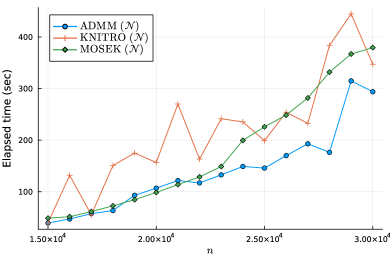
(a) random instances

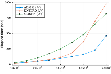
(b) linear-response model

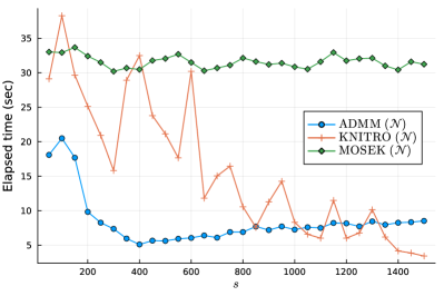
(c) real data set, $n=2000$

Figure 1: Computing the natural bound ($\mathcal{N}$) for D-Opt

4.2 MESP

We conducted two experiments to test the ADMM algorithm described in §3, to compute the factorization bound from DDFact for MESP. For these experiments, we considered an $n=2000$ covariance matrix with rank 949 based on Reddit data from [DMW21] and [BKDC17], and also used by [LX23] and [CFL23].

Before presenting our results, some observations should be made. We first note that, for all instances tested, the inequality (16) always holds, and therefore the integer $\hat{\jmath}$ considered in Lemma 3 exists. Thus, we can successfully solve subproblems (15) with the closed-form solution presented in Theorem 3.11. Nevertheless, if this were not the case, we could use an iterative algorithm to solve the subproblem for which $\hat{\jmath}$ could not be computed, for example, from KNITRO. Furthermore, we note that Proposition 2 is defined for $Z\in\mathbb{S}_{+}$ , and from Lemma 8 we may have $\lambda\not\geq 0$. In this case, we project $\lambda$ onto the nonnegative orthant and then apply Theorem 3.11 to construct $Z^{t+1}$. For the instances tested, we do get $\lambda$ with negative components, but they are always close to zero and the projection does not impact the convergence of the ADMM algorithm.

In our first experiment, to analyze the performance impact of the rank of $C$, we constructed matrices with rank $r=30,40,\ldots,300$, derived from the benchmark $n=2000$ covariance matrix by selecting its $r$-largest principal components. For all $r$, we set $s:=30$. The results are in Fig. 2. In the first plot, we have the times for our ADMM algorithm to solve DDFact, and compare them to the times for KNITRO to solve the two relaxations considered for MESP, namely DDFact and linx. We do not present times for the ADMM algorithm for linx discussed in §3.1, because they are not competitive. The bottleneck is the solution of the BVLS problem in (9), where the number of rows of the matrix $H$ is $\sim\!n^{2}$. However, the ADMM algorithm for linx could become competitive if we could solve this subproblem in a more efficient way, and therefore we discuss it in §3.1. The times in the first plot of Fig. 2 show that the ADMM algorithm is very efficient for DDFact for our instances, which could be solved faster than both relaxations for MESP considered when applying KNITRO. Furthermore, it is interesting to see in the second plot in Fig. 1, that for the instances considered, DDFact gives a better bound than linx. The gaps presented in the figure are computed as the difference between the upper bounds given by the dual solution of the relaxations and lower bounds computed by a local-search heuristic for MESP (see e.g., [KLQ95], for more details on the heuristic). Finally, we note that the time to solve DDFact with our ADMM algorithm generally increases with the rank $r$ of $C$, but it is always less than the KNITRO time to solve either DDFact or linx. We observe that the case where $r=s$ is more difficult for all algorithms and bounds, and lead to a bigger gap.

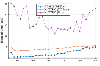
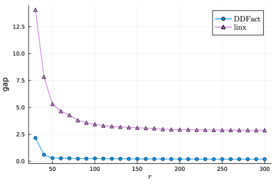
Figure 2: Computing MESP bounds, varying $r:=\operatorname{rank}(C)$ ($n=2000$, $s=30$)

In the second experiment, we aim at analyzing the impact of $s$ on the performance of the ADMM algorithm. In this case, we fix $r:=200$ and we consider $s=10,20,\dots,200$. In Fig. 3, we have similar results to the ones in Fig. 2, but now varying $s$ instead of $r$. The analysis of the results is very similar to the previous experiment. We again have a very effective application of the ADMM algorithm and see the difficulty of the problem generally increasing with $s$, with a particular high increase when $s=r$.

Finally, we observe in Figs. 2 and 3, varying both $r$ and $s$, we have, in general, a more stable behavior of the times for our ADMM algorithm than for KNITRO, as we have observed in Fig. 1 as well.

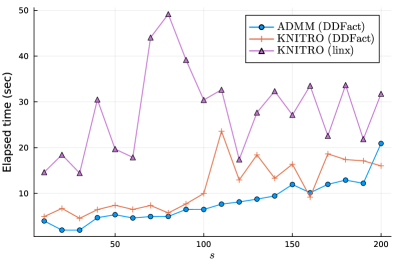
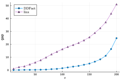
Figure 3: Computing MESP bounds, varying $s$ ($n=2000$, $\operatorname{rank}(C)=200$)

Appendix

Proof (of Proposition 1)

It suffices to show that $Z^{t+1}$ satisfies the first-order optimality condition of $\min_{Z}\{\!-\operatorname{ldet}(Z)\!+\!\frac{\rho}{2}\!\left\|Z\!-\!Y^{t+1}\right\|^{2}_{F}\}$, which is obtained by setting the gradient of the objective function equal to zero, that is,

$$-Z^{-1}+\rho(Z-Y^{t+1})=0,$$ (18)

together with the implicit constraint $Z\succ 0$. W can rewrite (18) as

$$\rho Z-Z^{-1}=\rho Y^{t+1}\Leftrightarrow\rho Z-Z^{-1}=Q\Theta Q^{\mathchoice{\raisebox{0.0pt}{$\displaystyle\scriptscriptstyle\mathsf{T}$}}{\raisebox{0.0pt}{$\textstyle\scriptscriptstyle\mathsf{T}$}}{\raisebox{0.0pt}{$\scriptstyle\scriptscriptstyle\mathsf{T}$}}{\raisebox{0.0pt}{$\scriptscriptstyle\scriptscriptstyle\mathsf{T}$}}}\Leftrightarrow\rho Q^{\mathchoice{\raisebox{0.0pt}{$\displaystyle\scriptscriptstyle\mathsf{T}$}}{\raisebox{0.0pt}{$\textstyle\scriptscriptstyle\mathsf{T}$}}{\raisebox{0.0pt}{$\scriptstyle\scriptscriptstyle\mathsf{T}$}}{\raisebox{0.0pt}{$\scriptscriptstyle\scriptscriptstyle\mathsf{T}$}}}ZQ-Q^{\mathchoice{\raisebox{0.0pt}{$\displaystyle\scriptscriptstyle\mathsf{T}$}}{\raisebox{0.0pt}{$\textstyle\scriptscriptstyle\mathsf{T}$}}{\raisebox{0.0pt}{$\scriptstyle\scriptscriptstyle\mathsf{T}$}}{\raisebox{0.0pt}{$\scriptscriptstyle\scriptscriptstyle\mathsf{T}$}}}Z^{-1}Q=\Theta.$$

From the orthogonality of $Q$, we can verify that the last equation is satisfied by $Z:=Q\Lambda Q^{\mathchoice{\raisebox{0.0pt}{$\displaystyle\scriptscriptstyle\mathsf{T}$}}{\raisebox{0.0pt}{$\textstyle\scriptscriptstyle\mathsf{T}$}}{\raisebox{0.0pt}{$\scriptstyle\scriptscriptstyle\mathsf{T}$}}{\raisebox{0.0pt}{$\scriptscriptstyle\scriptscriptstyle\mathsf{T}$}}}$ where $\Lambda:=\operatorname{\textstyle{Diag}}(\lambda_{1}\,\ldots,\lambda_{m})$ is an $m\times m$ diagonal matrix such that $\rho\lambda_{\ell}-1/\lambda_{\ell}=\theta_{\ell}$ for $\ell=1,\dots,m$. Thus, we have

$$\lambda_{\ell}=\frac{\theta_{\ell}+\sqrt{\theta_{\ell}^{2}+4\rho}}{2\rho},\quad\mbox{ for }\ell=1,\dots,m.$$

which are always positive since $\rho>0$. The result follows.         

Proof (of Corollary 2)

From (4), we can directly obtain the eigendecomposition of $\Psi^{t+1}$, given the eigendecompositions of $Z^{t+1}$ and $\rho Y^{t+1}$. Moreover, noticing that the function $f_{\rho}:\mathbb{R}\rightarrow\mathbb{R}$ defined by $f_{\rho}(a):=-a+\sqrt{a^{2}+4\rho}$ is decreasing in $a$, we verify that $\nu_{1}\leq\nu_{2}\leq\dots\leq\nu_{m}\,$.         

Proof (of Lemma 3)

Consider the function

$$f_{\rho}(x):=x+\sqrt{x^{2}+4\rho},$$

which is increasing in $x$. Then

$$f_{\rho}(x)=\frac{4\rho}{-x+\sqrt{x^{2}+4\rho}}\Rightarrow-x+\sqrt{x^{2}+4\rho}=\frac{4\rho}{f_{\rho}(x)}\Rightarrow x=\frac{1}{2}\left(f_{\rho}(x)-\frac{4\rho}{f_{\rho}(x)}\right).$$

For $\tau>0$, let $x_{\tau}$ be the value such that $f_{\rho}(x_{\tau})=\tau f_{\rho}(x)$. Then

$$x_{\tau}=\frac{1}{2}\left(f_{\rho}(x_{\tau})-\frac{4\rho}{f_{\rho}(x_{\tau})}\right)=\frac{1}{2}\left(\tau f_{\rho}(x)-\frac{4\rho}{\tau f_{\rho}(x)}\right).$$

As $\frac{4\rho}{f_{\rho}(x)}=f_{\rho}(x)-2x$, we have

$$x_{\tau}=\frac{1}{2}\left(\tau f_{\rho}(x)-\frac{1}{\tau}f_{\rho}(x)+\frac{2x}{\tau}\right)=\frac{x}{\tau}-\frac{1-\tau^{2}}{2\tau}f_{\rho}(x).$$

The middle term in the lemma is

$$\frac{1}{s-j}\sqrt{(k-j)(s-j)}\;f_{\rho}\left(\frac{\sum_{\ell=j+1}^{k}\theta_{\ell}}{\sqrt{(k-j)(s-j)}}\right)$$

$$\qquad\qquad=\sqrt{\frac{k-j}{s-j}}\;f_{\rho}\left(\frac{\sum_{\ell=j+1}^{k}\theta_{\ell}}{\sqrt{(k-j)(s-j)}}\right)$$

$$\qquad\qquad=\sqrt{\frac{k-j}{s-j}}\;f_{\rho}\left(\sqrt{\frac{k-j}{s-j}}\;\frac{\sum_{\ell=j+1}^{k}\theta_{\ell}}{k-j}\right).$$

Now let $\tau:=1\Big{/}\sqrt{\frac{k-j}{s-j}}$, and consider $\tau f_{\rho}(x)$, for $x=\theta_{j}$ and $x=\theta_{j+1}$ . We have

$$\tau f_{\rho}(\theta_{j})=f_{\rho}\left(\sqrt{\frac{k-j}{s-j}}\left(\theta_{j}-\frac{1-\frac{s-j}{k-j}}{2}f_{\rho}(\theta_{j})\right)\right),$$

$$\tau f_{\rho}(\theta_{j+1})=f_{\rho}\left(\sqrt{\frac{k-j}{s-j}}\left(\theta_{j+1}-\frac{1-\frac{s-j}{k-j}}{2}f_{\rho}(\theta_{j+1})\right)\right).$$

The lemma asks for $j$ such that

$$f_{\rho}(\theta_{j})>\frac{1}{\tau}\;f_{\rho}\left(\sqrt{\frac{k-j}{s-j}}\frac{\sum_{\ell=j+1}^{k}\theta_{\ell}}{k-j}\right)\geq f_{\rho}(\theta_{j+1})$$

$$\qquad\Leftrightarrow f_{\rho}\left(\sqrt{\frac{k-j}{s-j}}\left(\theta_{j}-\frac{1-\frac{s-j}{k-j}}{2}f_{\rho}(\theta_{j})\right)\right)$$

$$\qquad\qquad\qquad>f_{\rho}\left(\sqrt{\frac{k-j}{s-j}}\;\frac{\sum_{\ell=j+1}^{k}\theta_{\ell}}{k-j}\right)$$

$$\qquad\qquad\qquad\geq f_{\rho}\left(\sqrt{\frac{k-j}{s-j}}\left(\theta_{j+1}-\frac{1-\frac{s-j}{k-j}}{2}f_{\rho}(\theta_{j+1})\right)\right)$$

Because $f_{\rho}$ is increasing, this is if and only if

$$\theta_{j}-\frac{k-s}{2(k-j)}f_{\rho}(\theta_{j})>\frac{1}{k-j}\sum_{\ell=j+1}^{k}\theta_{\ell}\geq\theta_{j+1}-\frac{k-s}{2(k-j)}f_{\rho}(\theta_{j+1})$$

$$\Leftrightarrow(k-j)\theta_{j}-\frac{k-s}{2}f_{\rho}(\theta_{j})>\sum_{\ell=j+1}^{k}\theta_{\ell}\geq(k-j)\theta_{j+1}-\frac{k-s}{2}f_{\rho}(\theta_{j+1}).$$

Then, the proof is done as we will take $j$ as

$$\hat{\jmath}:=\min\left\{j~{}:~{}\sum_{\ell=j+1}^{k}\theta_{\ell}\geq(k-j)\theta_{j+1}-\frac{k-s}{2}\;f_{\rho}(\theta_{j+1})\right\}.$$

Note that $\hat{\jmath}$ is well defined because the inequality above holds for some $j$ if and only if the right-hand inequality in (17) holds for the same $j$. As the right-hand inequality in (17) reduces to (16) when $j=s-1$, we are assured that $\hat{\jmath}$ exists.

If $\hat{\jmath}=0$, then the left-hand inequality also holds. Suppose now that $\hat{\jmath}>0$. We want to check that the left-hand inequality in (17) holds for $j=\hat{\jmath}-1$; we have

$$\sum_{\ell=\hat{\jmath}}^{k}\theta_{\ell}<\left(k-\left(\hat{\jmath}-1\right)\right)\theta_{\hat{\jmath}}-\frac{k-s}{2}f_{\rho}(\theta_{\hat{\jmath}})$$

$$\qquad\Leftrightarrow\sum_{\ell=\hat{\jmath}+1}^{k}\theta_{\ell}<\left(k-\hat{\jmath}\right)\theta_{\hat{\jmath}}-\frac{k-s}{2}f_{\rho}(\theta_{\hat{\jmath}}),$$

which holds if and only if the left-hand inequality in (17) holds for $j=\hat{\jmath}$.         

Proof (of Lemma 5)

Let us assume that (17) holds for $j=j_{1}$ and $j=j_{2}$ with $0\leq j_{1}<j_{2}<s$. Then,

$$\textstyle\theta_{j_{2}}\,+\,\sqrt{\theta_{j_{2}}^{2}+4\rho}\,\leq\,\theta_{j_{1}+1}\,+\,\sqrt{\theta_{j_{1}+1}^{2}+4\rho}\,,$$

and

$$(s-j_{2})\left(\theta_{j_{2}}+\sqrt{\theta_{j_{2}}^{2}+4\rho}\,\right)\leq(s-j_{2})\left(\theta_{j_{1}+1}+\sqrt{\theta_{j_{1}+1}^{2}+4\rho}\,\right)$$

$$\quad=(s-j_{1})\left(\theta_{j_{1}+1}+\sqrt{\theta_{j_{1}+1}^{2}+4\rho}\,\right)-(j_{2}-j_{1})\left(\theta_{j_{1}+1}+\sqrt{\theta_{j_{1}+1}^{2}+4\rho}\,\right)$$

$$\quad\leq\displaystyle\sum_{\ell=j_{1}+1}^{k}\theta_{\ell}+\sqrt{\left(\sum_{\ell=j_{1}+1}^{k}\theta_{\ell}\right)^{2}+4\rho(k-j_{1})(s-j_{1})}$$

$$\quad\qquad\qquad-(j_{2}-j_{1})\left(\theta_{j_{1}+1}+\sqrt{\theta_{j_{1}+1}^{2}+4\rho}\,\right)$$

$$\quad=\displaystyle\sum_{\ell=j_{1}+1}^{j_{2}}(\theta_{\ell}-\theta_{j_{1}+1})+\displaystyle\sum_{\ell=j_{2}+1}^{k}\theta_{\ell}+\sqrt{\left(\sum_{\ell=j_{1}+1}^{k}\theta_{\ell}\right)^{2}+4\rho(k-j_{1})(s-j_{1})}$$

$$\quad\qquad\qquad-\displaystyle\sum_{\ell=j_{1}+1}^{j_{2}}\sqrt{\theta_{j_{1}+1}^{2}+4\rho}$$

$$\quad\leq\displaystyle\sum_{\ell=j_{2}+1}^{k}\theta_{\ell}+\sqrt{\left(\sum_{\ell=j_{1}+1}^{k}\theta_{\ell}\right)^{2}+4\rho(k-j_{1})(s-j_{1})}-\displaystyle\sum_{\ell=j_{1}+1}^{j_{2}}\sqrt{\theta_{j_{1}+1}^{2}+4\rho}$$

$$\quad=\displaystyle\sum_{\ell=j_{2}+1}^{k}\theta_{\ell}+\sqrt{\left(\sum_{\ell=j_{1}+1}^{j_{2}}\theta_{\ell}+\sum_{\ell=j_{2}+1}^{k}\theta_{\ell}\right)^{2}+4\rho(k-j_{1})(s-j_{1})}$$

$$\quad\qquad\qquad-\displaystyle\sum_{\ell=j_{1}+1}^{j_{2}}\sqrt{\theta_{j_{1}+1}^{2}+4\rho}$$

$$\quad\leq\displaystyle\sum_{\ell=j_{2}+1}^{k}\theta_{\ell}+\sqrt{\left(\sum_{\ell=j_{1}+1}^{j_{2}}\theta_{\ell}\right)^{2}}+\sqrt{\left(\sum_{\ell=j_{2}+1}^{k}\theta_{\ell}\right)^{2}+4\rho(k-j_{1})(s-j_{1})}$$

$$\quad\qquad\qquad-\displaystyle\sum_{\ell=j_{1}+1}^{j_{2}}\sqrt{\theta_{j_{1}+1}^{2}+4\rho}$$

$$\quad\leq\displaystyle\sum_{\ell=j_{2}+1}^{k}\theta_{\ell}+\sqrt{\left(\sum_{\ell=j_{2}+1}^{k}\theta_{\ell}\right)^{2}+4\rho(k-j_{1})(s-j_{1})},$$

which contradicts the left-hand inequality in (17) for $j=j_{2}$ .         

Proof (of Lemma 7)

When $s=k$ and $j=\xi$, the middle term in (17) reduces to $\theta_{\xi+1}+\sqrt{\theta_{\xi+1}^{2}+4\rho}$. Therefore, we can easily see that both inequalities in (17) hold. The uniqueness of $j$ is derived from Lemma 5.         

Proof (of Lemma 8)

Because $\theta_{1}\geq\theta_{2}\geq\dots\geq\theta_{k}$ , we have $\lambda_{1}\geq\lambda_{2}\geq\dots\geq\lambda_{\hat{\jmath}}$ and $\lambda_{\hat{\jmath}+1}\geq\lambda_{\hat{\jmath}+2}\geq\dots\geq\lambda_{k}$ . Now we just need to show that $\lambda_{\hat{\jmath}}>{\frac{\phi}{2\rho(s-\hat{\jmath})}\geq}\lambda_{\hat{\jmath}+1}$ . From the left-hand inequality in (17), we have that $\theta_{\hat{\jmath}}+\sqrt{\theta_{\hat{\jmath}}^{2}+4\rho}>\frac{\phi}{s-{\hat{\jmath}}}$, then

$$\lambda_{\hat{\jmath}}=\frac{\theta_{\hat{\jmath}}+\sqrt{\theta_{\hat{\jmath}}^{2}+4\rho}}{2\rho}>\frac{\phi}{2\rho(s-{\hat{\jmath}})}.$$

Now, define $w:=\frac{\phi}{s-{\hat{\jmath}}}$. Then, to show that

$$\frac{\phi}{2\rho(s-{\hat{\jmath}})}\geq\lambda_{{\hat{\jmath}}+1}\,,$$

it suffices to verify that

$$\frac{w}{2\rho}\geq\frac{\theta_{{\hat{\jmath}}+1}}{\rho}+\frac{2}{w}\;\Leftrightarrow\;w^{2}-2\theta_{{\hat{\jmath}}+1}w-{4\rho}\geq 0\,\Leftrightarrow$$

$$\left(w-{(\theta_{{\hat{\jmath}}+1}+\sqrt{\theta_{{\hat{\jmath}}+1}^{2}+4\rho})}\right)\left(w-{(\theta_{{\hat{\jmath}}+1}-\sqrt{\theta_{{\hat{\jmath}}+1}^{2}+4\rho})}\right)\geq 0.$$

From the right-hand inequality in (17), we have $w\geq\theta_{{\hat{\jmath}}+1}+\sqrt{\theta_{{\hat{\jmath}}+1}^{2}+4\rho}$ . Then

$$w\geq{\theta_{{\hat{\jmath}}+1}+\sqrt{\theta_{{\hat{\jmath}}+1}^{2}+4\rho}}\geq{\theta_{{\hat{\jmath}}+1}-\sqrt{\theta_{{\hat{\jmath}}+1}^{2}+4\rho}}\,.$$

Therefore, the result follows.         

Proof (of Lemma 9)

If $\theta_{\xi+1}\geq 0$, then $\theta\in\mathbb{R}^{k}_{+}$ and the result trivially follows. Therefore, in the following, we consider that $\theta_{\xi+1}<0$.

From Lemma 7, we know that $\xi$ is the unique integer that satisfies (17), i.e., $\hat{\jmath}=\xi$ in Lemma 8. It is straightforward to see that $\lambda_{\ell}>0$ for $\ell=1,\ldots,\hat{\jmath}$. So, it remains to prove that $\lambda_{\ell}>0$ for $\ell=\hat{\jmath}+1,\ldots,k$. We have that

$$\lambda_{\ell} =\frac{\theta_{\ell}}{\rho}+\frac{2(s-\hat{\jmath})}{\phi}$$

$$=\frac{\theta_{\ell}}{\rho}+\frac{2(k-\xi)}{(k-\xi)\theta_{\xi+1}+\sqrt{(k-\xi)^{2}\theta_{\xi+1}^{2}+4\rho(k-\xi)^{2}}}$$

$$=\frac{\theta_{\ell}}{\rho}+\frac{2}{\theta_{\xi+1}+\sqrt{\theta_{\xi+1}^{2}+4\rho}}$$

$$=\tilde{\theta}_{\ell}+\frac{2}{\rho\tilde{\theta}_{\xi+1}+\sqrt{\rho^{2}\tilde{\theta}_{\xi+1}^{2}+4\rho}}.$$

We see from the last expression that $\lambda_{\ell}=\lambda_{\ell}(\rho)$ is a decreasing function of $\rho$. Then, if suffices to show that $\lim_{\rho\rightarrow+\infty}\lambda_{\ell}(\rho)=0$, which holds because

$$\lim_{\rho\rightarrow+\infty}\left(-\tilde{\theta}_{\ell}\right)\left(\rho\tilde{\theta}_{\xi+1}+\sqrt{\rho^{2}\tilde{\theta}_{\xi+1}^{2}+4\rho}\right)=\lim_{\rho\rightarrow+\infty}-\rho\tilde{\theta}^{2}_{\xi+1}+\sqrt{\rho^{2}\tilde{\theta}_{\xi+1}^{4}+4\rho\tilde{\theta}_{\xi+1}^{2}}$$

$$\qquad=\lim_{\tau\rightarrow+\infty}-\tau+\sqrt{\tau^{2}+4\tau}=\lim_{\tau\rightarrow+\infty}\frac{\tau^{2}+4\tau-\tau^{2}}{\tau+\sqrt{\tau^{2}+4\tau}}$$

$$\qquad=\lim_{\tau\rightarrow+\infty}\frac{4}{1+\sqrt{1+4/\tau}}=2.$$

        

Proof (of Lemma 10)

From Lemma 8, we have

$$\lambda_{\hat{\jmath}}>\frac{\phi}{(s-{\hat{\jmath}})2\rho}\geq\lambda_{{\hat{\jmath}}+1}\,.$$

Now, let $\zeta:=\sum_{\ell={\hat{\jmath}}+1}^{k}\theta_{\ell}$ . Then, we have

$$\sum_{\ell={\hat{\jmath}}+1}^{k}\lambda_{\ell} =\frac{\zeta}{\rho}+\frac{2(k-{\hat{\jmath}})(s-{\hat{\jmath}})}{\zeta+\sqrt{\zeta^{2}+4\rho(k-{\hat{\jmath}})(s-{\hat{\jmath}})}}$$

$$=\frac{\zeta^{2}+\zeta\sqrt{\zeta^{2}+4\rho(k-{\hat{\jmath}})(s-{\hat{\jmath}})}+2\rho(k-{\hat{\jmath}})(s-{\hat{\jmath}})}{\rho(\zeta+\sqrt{\zeta^{2}+4\rho(k-{\hat{\jmath}})(s-{\hat{\jmath}})})}$$

$$=\frac{\zeta^{2}+2\zeta\sqrt{\zeta^{2}+4\rho(k-{\hat{\jmath}})(s-{\hat{\jmath}})}+\left(\zeta^{2}+4\rho(k-{\hat{\jmath}})(s-{\hat{\jmath}})\right)}{2\rho(\zeta+\sqrt{\zeta^{2}+4\rho(k-{\hat{\jmath}})(s-{\hat{\jmath}})})}$$

$$=\frac{\left(\zeta+\sqrt{\zeta^{2}+4\rho(k-{\hat{\jmath}})(s-{\hat{\jmath}})}\right)^{2}}{2\rho(\zeta+\sqrt{\zeta^{2}+4\rho(k-{\hat{\jmath}})(s-{\hat{\jmath}})})}$$

$$=\frac{\zeta+\sqrt{\zeta^{2}+4\rho(k-{\hat{\jmath}})(s-{\hat{\jmath}})}}{2\rho}$$

$$=\frac{\phi}{2\rho}.$$

Therefore, we can see that the unique integer $\hat{\imath}$ defined for $\lambda$ by Lemma 1 is exactly ${\hat{\jmath}}$.         

Proof (of Theorem 3.11)

Let ${\hat{\jmath}}$ be the unique integer defined by Lemma 3. In Lemma 10, we showed that ${\hat{\jmath}}$ is $\hat{\imath}$ defined by Lemma 1 for $\lambda$. Therefore, from Proposition 2, we have that $Q\operatorname{\textstyle{Diag}}(\beta)Q^{\mathchoice{\raisebox{0.0pt}{$\displaystyle\scriptscriptstyle\mathsf{T}$}}{\raisebox{0.0pt}{$\textstyle\scriptscriptstyle\mathsf{T}$}}{\raisebox{0.0pt}{$\scriptstyle\scriptscriptstyle\mathsf{T}$}}{\raisebox{0.0pt}{$\scriptscriptstyle\scriptscriptstyle\mathsf{T}$}}}\in\partial\Gamma_{s}(Z^{t+1}),$ where

$$\beta_{\ell}:=\begin{cases}\displaystyle\frac{1}{\lambda_{\ell}},\quad&\ell=1,\dots,{\hat{\jmath}};\\[10.0pt] \displaystyle\frac{2\rho(s-{\hat{\jmath}})}{\phi},\quad&\ell={\hat{\jmath}}+1,\dots,k,\end{cases}$$

where $\phi$ is defined in Lemma 8.

Let $f(Z):=-\Gamma_{s}(Z)+\frac{\rho}{2}\|Z-Y^{t+1}\|_{F}^{2}$ . Note that

$$\partial f(Z^{t+1}) \ni-Q\operatorname{\textstyle{Diag}}(\beta)Q^{\mathchoice{\raisebox{0.0pt}{$\displaystyle\scriptscriptstyle\mathsf{T}$}}{\raisebox{0.0pt}{$\textstyle\scriptscriptstyle\mathsf{T}$}}{\raisebox{0.0pt}{$\scriptstyle\scriptscriptstyle\mathsf{T}$}}{\raisebox{0.0pt}{$\scriptscriptstyle\scriptscriptstyle\mathsf{T}$}}}+\rho(Z^{t+1}-Y^{t+1})$$

$$=-Q\operatorname{\textstyle{Diag}}(\beta)Q^{\mathchoice{\raisebox{0.0pt}{$\displaystyle\scriptscriptstyle\mathsf{T}$}}{\raisebox{0.0pt}{$\textstyle\scriptscriptstyle\mathsf{T}$}}{\raisebox{0.0pt}{$\scriptstyle\scriptscriptstyle\mathsf{T}$}}{\raisebox{0.0pt}{$\scriptscriptstyle\scriptscriptstyle\mathsf{T}$}}}+\rho Q\operatorname{\textstyle{Diag}}(\lambda)Q^{\mathchoice{\raisebox{0.0pt}{$\displaystyle\scriptscriptstyle\mathsf{T}$}}{\raisebox{0.0pt}{$\textstyle\scriptscriptstyle\mathsf{T}$}}{\raisebox{0.0pt}{$\scriptstyle\scriptscriptstyle\mathsf{T}$}}{\raisebox{0.0pt}{$\scriptscriptstyle\scriptscriptstyle\mathsf{T}$}}}-Q\Theta Q^{\mathchoice{\raisebox{0.0pt}{$\displaystyle\scriptscriptstyle\mathsf{T}$}}{\raisebox{0.0pt}{$\textstyle\scriptscriptstyle\mathsf{T}$}}{\raisebox{0.0pt}{$\scriptstyle\scriptscriptstyle\mathsf{T}$}}{\raisebox{0.0pt}{$\scriptscriptstyle\scriptscriptstyle\mathsf{T}$}}}$$

$$=Q\operatorname{\textstyle{Diag}}(\rho\lambda-\beta-\theta)Q^{\mathchoice{\raisebox{0.0pt}{$\displaystyle\scriptscriptstyle\mathsf{T}$}}{\raisebox{0.0pt}{$\textstyle\scriptscriptstyle\mathsf{T}$}}{\raisebox{0.0pt}{$\scriptstyle\scriptscriptstyle\mathsf{T}$}}{\raisebox{0.0pt}{$\scriptscriptstyle\scriptscriptstyle\mathsf{T}$}}}.$$

It suffices to show that $0\in\partial f(Z^{t+1})$, and hence it suffices to show that $\rho\lambda_{\ell}-\beta_{\ell}-\theta_{\ell}=0$ for $\ell=1,\dots,k$. For $\ell=1,\dots,{\hat{\jmath}}$, we have

$$\rho\lambda_{\ell}-\frac{1}{\lambda_{\ell}}-\theta_{\ell} =\rho\frac{\theta_{\ell}+\sqrt{\theta_{\ell}^{2}+4\rho}}{2\rho}-\frac{2\rho}{\theta_{\ell}+\sqrt{\theta_{\ell}^{2}+4\rho}}-\theta_{\ell}$$

$$=\frac{\left({\theta_{\ell}+\sqrt{\theta_{\ell}^{2}+4\rho}}\right)^{2}-\left(\theta_{\ell}^{2}+2\theta_{\ell}\sqrt{\theta_{\ell}^{2}+4\rho}+(\theta_{\ell}^{2}+4\rho)\right)}{2\theta_{\ell}+2\sqrt{\theta_{\ell}^{2}+4\rho}}$$

$$=\frac{\left({\theta_{\ell}+\sqrt{\theta_{\ell}^{2}+4\rho}}\right)^{2}-\left({\theta_{\ell}+\sqrt{\theta_{\ell}^{2}+4\rho}}\right)^{2}}{2\theta_{\ell}+2\sqrt{\theta_{\ell}^{2}+4\rho}}=0.$$

For $\ell={\hat{\jmath}}+1,\dots,k$, we have

$$\rho\lambda_{\ell}-\frac{2\rho(s-{\hat{\jmath}})}{\phi}-\theta_{\ell} =\rho\frac{\theta_{\ell}}{\rho}+\rho\frac{2(s-{\hat{\jmath}})}{\phi}-\frac{2\rho(s-{\hat{\jmath}})}{\phi}-\theta_{\ell}=0,$$

and therefore $0\in\partial f(Z^{t+1})$.         

Proof (of Corollary 12)

From (13), we have $\Psi^{t+1}:=\Psi^{t}-F^{\mathchoice{\raisebox{0.0pt}{$\displaystyle\scriptscriptstyle\mathsf{T}$}}{\raisebox{0.0pt}{$\textstyle\scriptscriptstyle\mathsf{T}$}}{\raisebox{0.0pt}{$\scriptstyle\scriptscriptstyle\mathsf{T}$}}{\raisebox{0.0pt}{$\scriptscriptstyle\scriptscriptstyle\mathsf{T}$}}}\operatorname{\textstyle{Diag}}(x^{t+1})F+Z^{t+1}=Z^{t+1}-Y^{t+1}$. Following the construction of $Z^{t+1}$ using $\lambda$ defined in Lemma 8, we have $\Psi^{t+1}=Q\operatorname{\textstyle{Diag}}(\lambda-\frac{1}{\rho}\theta)Q^{\mathchoice{\raisebox{0.0pt}{$\displaystyle\scriptscriptstyle\mathsf{T}$}}{\raisebox{0.0pt}{$\textstyle\scriptscriptstyle\mathsf{T}$}}{\raisebox{0.0pt}{$\scriptstyle\scriptscriptstyle\mathsf{T}$}}{\raisebox{0.0pt}{$\scriptscriptstyle\scriptscriptstyle\mathsf{T}$}}}$, then we define $\nu:=\lambda-\frac{1}{\rho}\theta$. Note that for $\ell=1,\dots,\hat{\jmath}$

$$\nu_{\ell}=\frac{\theta_{\ell}+\sqrt{\theta_{\ell}^{2}+4\rho}}{2\rho}-\frac{\theta_{\ell}}{\rho}=\frac{-\theta_{\ell}+\sqrt{\theta_{\ell}^{2}+4\rho}}{2\rho}\,,$$

for $\ell=\hat{\jmath}+1,\dots,k$

$$\nu_{\ell}=\frac{\theta_{\ell}}{\rho}+\frac{2(s-\hat{\jmath})}{\phi}-\frac{\theta_{\ell}}{\rho}=\frac{2(s-\hat{\jmath})}{\phi}\,.$$

Also, we note that because $\rho>0$ and $0\leq\hat{\jmath}<s\leq k$, then $\nu>0$. Finally, we note that the function $f_{\rho}:\mathbb{R}\rightarrow\mathbb{R}$, defined by $f_{\rho}(a):=-a+\sqrt{a^{2}+4\rho}$, is decreasing in $a$, so $\nu_{1}\leq\dots\leq\nu_{\hat{\jmath}}\,.$ Then, it suffices to show that $\frac{-\theta_{\hat{\jmath}}+\sqrt{\theta_{\hat{\jmath}}^{2}+4\rho}}{2\rho}\leq 2(s-\hat{\jmath})/\phi\,.$ Suppose by contradiction that

$$\frac{-\theta_{\hat{\jmath}}+\sqrt{\theta_{\hat{\jmath}}^{2}+4\rho}}{2\rho}>\frac{2(s-\hat{\jmath})}{\phi}\,.$$

From Lemma 8 we have $\lambda_{\hat{\jmath}}=\frac{\theta_{\hat{\jmath}}+\sqrt{\theta_{\hat{\jmath}}^{2}+4\rho}}{2\rho}>\frac{\phi}{2\rho(s-\hat{\jmath})}\Leftrightarrow\frac{2(s-\hat{\jmath})}{\phi}>\frac{2}{\theta_{\hat{\jmath}}+\sqrt{\theta_{\hat{\jmath}}^{2}+4\rho}}\,.$ Then, we have

$$\frac{-\theta_{\hat{\jmath}}+\sqrt{\theta_{\hat{\jmath}}^{2}+4\rho}}{2\rho}>\frac{2}{\theta_{\hat{\jmath}}+\sqrt{\theta_{\hat{\jmath}}^{2}+4\rho}}\Leftrightarrow$$

$$-\theta^{2}_{\hat{\jmath}}+\theta_{\hat{\jmath}}^{2}+4\rho>4\rho\Leftrightarrow$$

$$4\rho>4\rho\,.$$

The contradiction completes the proof.

References

[Ans20]
Kurt M. Anstreicher.
Efficient solution of maximum-entropy sampling problems.
Operations Research, 68(6):1826–1835, 2020.
https://doi.org/10.1287/opre.2019.1962.
[BBC+08]
Pierre Bonami, Lorenz T. Biegler, Andrew R. Conn, Gérard Cornuéjols, Ignacio E. Grossmann, Carl D. Laird, Jon Lee, Andrea Lodi, François Margot, Nicolas Sawaya, and Andreas Wächter.
An algorithmic framework for convex mixed integer nonlinear programs.
Discrete Optimization, 5(2):186–204, 2008.
https://doi.org/10.1016/j.disopt.2006.10.011.
[BKDC17]
Shrey Bagroy, Ponnurangam Kumaraguru, and Munmun De Choudhury.
A social media based index of mental well-being in college campuses.
In Proceedings of the 2017 CHI Conference on Human Factors in Computing Systems, pages 1634–1646. Association for Computing Machinery, 2017.
https://doi.org/10.1145/3025453.3025909.
[BPC+11]
Stephen Boyd, Neal Parikh, Eric Chu, Borja Peleato, and Jonathan Eckstein.
Distributed optimization and statistical learning via the alternating direction method of multipliers.
Foundations and Trends in Machine Learning, 3(1):1–122, 2011.
https://doi.org/10.1561/2200000016.
[CFL23]
Zhongzhu Chen, Marcia Fampa, and Jon Lee.
On computing with some convex relaxations for the maximum-entropy sampling problem.
INFORMS Journal on Computing, 35:368–385, 2023.
https://doi.org/10.1287/ijoc.2022.1264.
[CFL24]
Zhongzhu Chen, Marcia Fampa, and Jon Lee.
Generalized scaling for the constrained maximum-entropy sampling problem.
Mathematical Programming, 2024.
https://doi.org/10.1007/s10107-024-02101-3.
[DMW21]
Santanu S. Dey, Rahul Mazumder, and Guanyi Wang.
Using -relaxation and integer programming to obtain dual bounds for sparse PCA.
Operations Research (in press), 2021.
[LX23]
Yongchun Li and Weijun Xie.
Best principal submatrix selection for the maximum entropy sampling problem: Scalable algorithms and performance guarantees.
Operations Research, 72(2):493–513, 2023.
https://doi.org/10.1287/opre.2023.2488.
[Nik15]
Aleksandar Nikolov.
Randomized rounding for the largest simplex problem.
In Proceedings of STOC 2015, pages 861–870. ACM, 2015.
https://doi.org/10.1145/2746539.2746628.
[NNN+21]
Takayuki Nagata, Taku Nonomura, Kumi Nakai, Keigo Yamada, Yuji Saito, and Shunsuke Ono.
Data-driven sparse sensor selection based on A-optimal design of experiment with ADMM.
IEEE Sensors Journal, 21(13):15248–15257, 2021.
https://doi.org/10.1109/JSEN.2021.3073978.
[PFL23]
Gabriel Ponte, Marcia Fampa, and Jon Lee.
Branch-and-bound for D-optimality with fast local search and variable-bound tightening, 2023.
Preprint: https://arxiv.org/abs/2309.00117.
[PFL24]
Gabriel Ponte, Marcia Fampa, and Jon Lee.
Convex relaxation for the generalized maximum-entropy sampling problem, 2024.
https://arxiv.org/abs/2404.01390.
[SMG10]
Katya Scheinberg, Shiqian Ma, and Donald Goldfarb.
Sparse inverse covariance selection via alternating linearization methods.
In Proceedings of the 23rd International Conference on Neural Information Processing Systems - Volume 2, NIPS’10, pages 2101–2109, Red Hook, NY, USA, 2010. Curran Associates Inc.
https://proceedings.neurips.cc/paper_files/paper/2010/file/2723d092b63885e0d7c260cc007e8b9d-Paper.pdf.