Helium as an Indicator of the Neutron-Star Merger Remnant Lifetime
and its Potential for Equation of State Constraints

Abstract

The time until black hole formation in a binary neutron-star (NS) merger contains invaluable information about the nuclear equation of state (EoS) but has thus far been difficult to measure. We propose a new way to constrain the merger remnant’s NS lifetime, which is based on the tendency of the NS remnant neutrino-driven winds to enrich the ejected material with helium. Based on the He i $\lambda 1083.3$ nm line, we show that the feature around 800–1200 nm in AT2017gfo at 4.4 days seems inconsistent with a helium mass fraction of $X_{\mathrm{He}}\gtrsim 0.05$ in the polar ejecta. Recent neutrino-hydrodynamic simulations of merger remnants are only compatible with this limit if the NS remnant collapses within 20–30 ms. Such a short lifetime implies that the total binary mass of GW170817, $M_{\mathrm{\rm tot}}$, lay close to the threshold binary mass for direct gravitational collapse, $M_{\mathrm{thres}}$, for which we estimate $M_{\mathrm{thres}}\lesssim 2.93\,M_{\odot}$. This upper bound on $M_{\mathrm{thres}}$ yields upper limits on the radii and maximum mass of cold, non-rotating NSs, which rule out simultaneously large values for both quantities. In combination with causality arguments, this result implies a maximum NS mass of $M_{\mathrm{max}}\lesssim 2.3\,M_{\odot}$. The combination of all limits constrains the radii of 1.6 M_⊙ NSs to about 12$\pm$1 km for $M_{\mathrm{max}}$ = 2.0 M_⊙ and 11.5$\pm$1 km for $M_{\mathrm{max}}$ = 2.15 M_⊙. This $\sim 2$ km allowable range then tightens significantly for $M_{\mathrm{max}}$ above $\approx 2.15$ M_⊙. This rules out a significant number of current EoS models. The short NS lifetime also implies that a black-hole torus, not a highly magnetized NS, was the central engine powering the relativistic jet of GRB170817A. Our work motivates future developments to further corroborate and improve uncertainties in our chain of arguments, regarding NLTE spectral modeling, helium production in merger outflows, and the dependence of the remnant lifetime on the binary mass, with the potential to tighten our constraints from existing data and in particular from future events. This novel method may provide a powerful tool to get a handle on the poorly constrained remnant lifetime, the still debated central engine of short GRBs, and the high-density EoS.

I Introduction

Neutron-star mergers (NSM) provide natural laboratories for studying the incompletely known properties of high-density matter quantified by the equation of state (EoS). The EoS relates the pressure and density of neutron-star matter, and is uniquely linked to the stellar parameters of neutron stars such as the mass-radius relation or the tidal deformability, measurements of which, in turn, constrain the EoS [1, 2, 3, 4, 5, 6, 7]. From the first gravitational-wave detected NSM-merger, GW170817, several binary parameters like the observer distance, the total binary mass, the binary mass ratio and the dimensionless tidal deformability, $\Lambda$, could be constrained [8, 9]. Since $\Lambda$ scales tightly with the NS radius, this has been constrained to be $\lesssim$ 13.5 km in the mass range around 1.4 M_⊙, which rules out very stiff models of high-density matter [10, 11].

GW170817 was accompanied by the kilonova (KN) AT2017gfo [12, 13, 14, 15, 16, 17, 18, 19, 20, 21, 22, 23, 24, 25, 26], i.e. optical/infrared emission resulting from radioactive decays connected to the rapid neutron-capture process (r-process [27, 28, 29]) in the matter outflows during and after the merger [30, 31, 32]. A large number of studies have since employed the properties of the kilonova to derive additional EoS constraints all relying on the fact that the merger dynamics and thus the matter ejection are sensitive to the EoS, and therefore the electromagnetic emission should carry an imprint of the properties of high-density matter.

Early on, the argument was made that GW170817 did not result in a prompt gravitational collapse to a black hole as the high brightness of AT2017gfo disfavors such a scenario, which would be accompanied with reduced ejecta mass and therefore relatively dim kilonova luminosity [33, 34, 35, 36, 37], but see [38]. This implies that the measured total binary mass of GW170817 was below the threshold binary mass for prompt collapse, which is an EoS-dependent quantity. Following this reasoning NS radii cannot be too small ($R\gtrsim 10.5$ km) and the EoS cannot be too soft, as this would have resulted in direct black hole (BH) formation [33, 39].

Several studies also presented arguments that a black hole did eventually form during the subsequent evolution of the rotating merger remnant. First, a NS remnant surviving longer than a few seconds or more should likely have injected a large fraction of its rotational energy through magnetic spindown [40] into the ejecta, which seems incompatible with the absence of a corresponding late-time signal in the electromagnetic emission [41, 42, 43, 44]. Second, the detection of a short gamma-ray burst (GRB) about 1.74 s after the GW signal provides an upper limit on the lifetime, if the GRB was launched by a black-hole torus system [45, 46, 43]. Assuming these arguments, the aforementioned studies find upper limits for the maximum mass of cold, non-rotating neutron stars (also known as the Tolman-Oppenheimer-Volkoff (TOV) limit) of about 2.17–2.3 M_⊙. However, the detailed evolution of NS remnants is currently not well understood due to the challenges in capturing all of the relevant physics (e.g. neutrino transport, small-scale turbulence, general relativity). As a consequence, the NS remnant lifetime, i.e. the black-hole formation time, $\tau_{\mathrm{BH}}$, in GW170817 is largely unconstrained to date, and it may even be $\tau_{\mathrm{BH}}>$ 1.7 s if the GRB signal originated from a highly magnetized NS remnant (“magnetar” scenario [47, 48, 49]).

A number of other studies, e.g. [50, 51, 52, 53, 54, 55, 56], employed the lightcurve and color evolution of the kilonova to directly link those features to NS parameters. Such an approach allows for efficient exploration of the large parameter space, but it suffers from significant systematic uncertainties, for instance, connected to the nuclear physics input, atomic data, radiative-transfer modeling, thermalization physics, or observation-angle dependence. The link between ejecta properties and the EoS is based entirely on predictions from numerical simulations, which again carry uncertainties that are difficult to quantify (numerical resolution dependence, neutrino transport physics, small-scale turbulence, approximate inclusions of long-term matter ejection; see also [57, 58, 59] illustrating some of the ambiguities).

In this paper we propose a conceptually new method based on the abundance of a specific element, namely helium, to constrain the lifetime of NS merger remnants. We present evidence that the remnant in GW170817 was only short-lived ($\lesssim 20$–$30$ ms). A remnant with longer lifetime would have resulted in a larger amount of helium, pronounced spectral features of which are, however, not found in the spectra. We use this argument to derive EoS constraints, specifically upper limits on NS radii and the maximum NS mass. In contrast to previous methodologies we employ for the first time information from the kilonova spectra to place constraints on NS parameters highlighting the value of the spectral information not only for nucleosynthesis but also for the merger dynamics and EoS. This work is a first exploratory study highlighting the idea and the potential of the method. Future work is needed to further corroborate and develop each of the steps taken in our study.

The paper is structured as follows. In Sect. II we describe the upper limit on the amount of helium in the outflow of AT2017gfo inferred from the spectral energy distribution. We review helium production in the outflows from neutron-star mergers based on theoretical models in Sect. III to deduce an upper limit of the remnant lifetime. The resulting constraints on NS parameters are presented in Sect. IV. In Sect. V we discuss additional implications of our analysis. We conclude in Sect. VI. In this paper we use the total binary mass $M_{\mathrm{tot}}=M_{1}+M_{2}$ with $M_{1,2}$ being the gravitational mass of NSs in a binary with infinite orbital separation. We define the binary mass ratio as $q=M_{1}/M_{2}$ with $M_{1}\leq M_{2}$, hence $q\leq 1$.

II The observational limits on helium production in AT2017gfo

Spectral modeling of kilonovae has seen major progress in recent years, largely motivated by the spectroscopic data-series from the kilonova AT2017gfo [e.g. 22, 21, 23] and AT2023vfi [60]. These spectra have already provided the first direct identification of known lines from r-process elements such as the identification of the most prominent component in the spectrum that lies around 1 $\upmu$m as an absorption-emission ‘P Cygni’ feature of the Sr ii triplet of strong lines (4p⁶4d-4p⁶5p) [61, 62, 63, 64, 65, 66]. Compelling cases for other line identifications have also been made, viz. Y ii [67], Te iii [68], La iii and Ce iii [69]. Given the limited atomic data, most kilonova modeling of spectral features has been done under the assumption of local thermodynamic equilibrium (LTE) [although, see 68, 70, 71, 72], but non-LTE (NLTE) effects are expected to be important for estimating level populations and ionisation states.

Coincidentally, He i $\lambda 1083.3$ nm (1s2s ³S–1s2p ³P) under NLTE conditions may also contribute to the 1 $\upmu$m feature. Perego et al. [73] initially concluded that the low helium abundance ($\lesssim 10^{-5}$ M_⊙) produced in the dynamical ejecta of their models could not explain the observed prominence of the feature. Tarumi et al. [74] concluded that relatively minor quantities of helium ($\sim 10^{-4}$ M_⊙) in their modeling could tentatively explain the observed feature at all epochs given sufficient UV line-blanketing. However, by accounting for higher energy levels and including UV flux detections from the Swift satellite, Sneppen et al. [75] showed that a helium interpretation is inconsistent with the 1 $\upmu$m feature in the first days post merger both in terms of its evolution and amplitude.

Nevertheless, at around 4–5 days post merger optimal conditions do arise for helium to produce a detectable spectral feature at this wavelength (see App. A.1). In Fig. 1, we show the 4.4 day spectra of AT2017gfo taken with the X-shooter spectrograph on the VLT, where there could be a contribution to the absorption feature at 800–1000 nm from He i. The absorption feature’s strength can be used to place a limit on the He i 1s2s ³S population in the line-forming region and hence on the total He i mass via non-LTE modeling. A priori we do not know the relative contribution of Sr ii and He i, so that the helium mass required to produce the observed feature may be considered an upper bound on the helium mass in that velocity range in AT2017gfo.

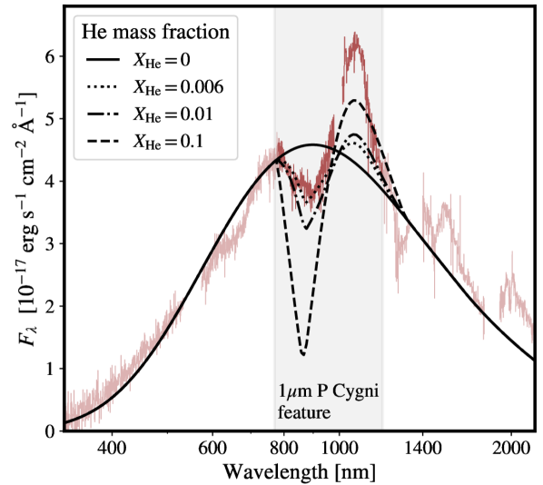
Figure 1: VLT/X-shooter spectrum of AT2017gfo 4.4 days post merger with a blackbody continuum overlaid ($T_{\rm BB}=3200$ K from the best-fit blackbody compilation in Sneppen et al. [66]) and P Cygni features for various helium abundances computed using the model described in Sect. II. Given a sufficient helium abundance, $X_{\rm He}\sim 0.01$, a sizeable absorption feature will be produced in the region 800–1000 nm. The other spectral features in the spectrum have been tentatively linked to Y ii (600–800 nm) and La iii, Ce iii, Te iii (1200–1600 nm, 2000 nm).

In the following sub-sections, we derive constraints on the maximally allowed helium mass fraction, $X_{\mathrm{He}}$, in the line-forming region following our modeling in [75]. First, we summarize the radiative-collisional model used to estimate the fraction of helium in the relevant lower level of the 1083 nm line (i.e. 1s2s ³S). Next, we outline the P Cygni modeling used to compare 1s2s ³S densities with the observed feature from which our $X_{\mathrm{He}}$ constraint is derived.

II.1 Modeling of NLTE helium level populations

To accurately model the NLTE population of 1s2s ³S, we compute a full collisional-radiative model analogous to previous studies of supernovae [e.g. 76] and of kilonovae [74]. Details on the computational modeling can be found in Sneppen et al. [75], but we note that the atomic data for helium is reliable (particularly in comparison to r-process elements) due to the substantiating experimental data, the multitude of prior applications (including in astrophysical contexts) and the simplicity of the few electron system for computational concerns. The atomic data employed includes $A$-values [77], thermally-averaged transition rates from collisions with electrons [78], recombination rates, and photoionisation cross-sections [79].

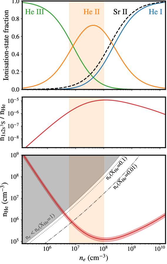
Figure 2: The fraction of helium in each ionisation state (top panel), the fraction of helium in the 1s2s ³S state (middle panel) and the helium density required to produce the observed feature (red line, bottom panel) as a function of photospheric electron density. All other parameters have their standard values, as described in App. A.2. For comparison, in the top panel, we also show the Sr ii fraction given a recombination rate, $\alpha=3\times 10^{-12}\,{\rm s}^{-1}\,{\rm cm}^{3}$. In the lower panel, dotted and dash-dotted lines shows $n_{e}$ as a function of $n_{\mathrm{He}}$ given various assumed $X_{\mathrm{He}}$ and adopting a mean mass, $A=100$, and same mean charge as helium for all other species. While the unphysical regime where $n_{e}$ is smaller than the electron density solely contributed by helium is shown in the grey shaded region. The electron densities expected near the photosphere (indicated with shaded orange region, $n_{e}\approx 6\times 10^{6}$–$10^{8}\ {\rm cm}^{-3}$, see App. A.3) predict He ii should constitute a major ionisation state and thus a sizeable population will be in 1s2s ³S. This implies i) a small density of helium, $n_{\mathrm{He}}\sim 10^{5}$–$10^{6}$ cm^-3 would be sufficient to produce the observed feature and ii) such electron density cannot solely be explained from the electrons contributed by helium ions, but require other ions.

In our models we assume homologously expanding ejecta with a power-law density dependence in velocity, $\rho=\rho_{0}v^{\alpha}$. The normalisation constant, $\rho_{0}$, is chosen such that the ejecta mass in the velocity range 0.1–0.5$c$ is 0.04 M_⊙, around the estimated ejecta mass for AT2017gfo [e.g. 25, 23]. We considered a large range of power-law slopes from constant density ($\alpha=0$) to steep declines ($\alpha=-5$) but adopt $\alpha=-5$ for our fiducial model (see App. A). We note this choice yields a mass for the high-velocity ejecta ($\gtrsim 0.2c$) of $\sim$0.01 M_⊙, which is consistent with observational constraints from AT2017gfo [e.g.  15, 80, 81]. The model assumes a uniform mass fraction of helium, $X_{\mathrm{He}}$, which is treated as a free parameter. The electron number density, $n_{e}$, is also assumed to follow the same velocity profile (i.e. $n_{e}\propto v^{\alpha}$) but with free normalisation. In all cases considered here, we will adopt a photospheric velocity at 4.4 days of $v_{\rm ph}=0.19c$ [75, we note a slightly lower value $\sim 0.15c$ can also be consistent with observations and would provide even stronger limits, see App. A.1], and place the outer boundary of the calculation at $v_{\rm max}=0.5c$. For the electron temperature, we assume, for the baseline model, the relativistically Doppler-corrected blackbody temperature, i.e. $T_{e}=2800$ K at 4.4 days (but explore a broader temperature range in App. A.4). We note, the relativistic Doppler-correction leads to a slight decrease from the observed blackbody temperature of $T_{\rm BB}=3200$ K. We also assume that the radiation field in the model is a dilute blackbody at the same temperature (again see Sneppen et al. [75] for details).

Each model involves solving the NLTE statistical equilibrium equations (see App. A.2) at each velocity point in the computational domain as input for the spectrum synthesis calculation discussed in Sect. II.2. However, it is instructive to consider behavior around the photosphere to illustrate when the line will appear. To this end, Fig. 2 shows, as a function of the adopted photospheric electron density (keeping everything else constant at their standard values, see App. A.2), the helium ionization state, occupation fraction for the 1s2s ³S level, and the helium density required for photospheric optical depth $\tau=0.86\pm 0.18$ (see below). As discussed by Sneppen et al. [75], the 1s2s ³S population is set by the balance between the outgoing pathways (i.e. decay to the He i ground state) versus the incoming recombination rate (which itself depends on the ionisation state of helium in the ejecta). The recombination rate is maximized, and thus the highest population in the 1s2s ³S state is achieved, when the majority of helium is singly ionized (see Fig. 2, top and middle panel). Conversely, the triplet population is minimal for either i) weak non-thermal ionisation (as fulfilled in the LTE limit where the He i ground state is the only significantly populated level) or ii) low electron densities and/or high non-thermal ionisation rates (i.e. the regime of He iii dominance).

Our estimate for the helium ionisation state in the ejecta for various electron densities is shown in Fig. 2 (top panel). Across a broad range of electron densities, $n_{e}\approx 10^{6}-10^{9}\,{\rm cm}^{-3}$ (which contains the likely $n_{e}$ of AT2017gfo at 4.4 days, see App. A.3), He ii will be a significant fraction of the total helium population. For this fiducial calculation we have used the deposition-rate of non-thermal particles, electrons and gammas, from [82] that is determined assuming the $\beta$-decay of an abundance pattern that reproduce the solar system r-process abundances, while weaker/stronger deposition rates of non-thermal particles are discussed in Sect. II.3. Regardless, for He ii to be significantly depleted would require either the electron density and/or the deposition rate to be orders-of-magnitude different from our fiducial expectation. For comparison, we show the corresponding Sr ii fraction assuming a work per ion of 300 eV and a recombination rate of $\alpha=3\times 10^{-12}\,{\rm s}^{-1}\,{\rm cm}^{3}$ at $T\approx 3000$ K [C. Ballance, personal communication]. While Sr ii is a sub-dominant ion state for the expected $n_{e}$ at 4.4 days post merger, its fraction is still substantial, and only modest amounts of Sr ii are needed to produce the observed feature with $M_{\rm\textup{Sr\,{ii}}}\sim 10^{-6}$–$10^{-5}M_{\odot}$ [61, 63].

II.2 P Cygni modeling

To compare the 1s2s ³S density with the observed feature, we will use the P Cygni implementation in the Elementary Supernova model, see ref. [83]. Specifically, assuming homologous expansion, the optical depth of the $\lambda_{0}=1083.3\,$nm line is simply related to the density in 1s2s ³S and the time post-merger by [84, 74]:

$$\tau_{\rm\textup{He\,{i}}\,\lambda 1083\,nm}(v)=\left(\frac{n_{\mathrm{1s2s\,^{3}S}}(v)}{\rm 7.4\ cm^{-3}}\right)\left(\frac{t}{\rm 1\,day}\right)$$ (1)

Thus, our NLTE populations allow us to compute the optical depth as a function of velocity from $v_{\rm ph}$ to $v_{\rm max}$ from which the P Cygni line profile is calculated.

Synthetic line profiles calculated in this way can then be compared to the observed 4.4 day spectrum to determine which models yield compatible optical depths, $\tau_{\rm\textup{He\,{i}}\,\lambda 1083\,nm}(v)$. Since this derives from $n_{\mathrm{1s2s\,^{3}S}}$, it in turn leads to a constraint on the He ii and total helium density via our modeling of the ionisation and excitation state of helium in the ejecta. A more detailed view of KN P Cygni modeling can be found in [85].

II.3 Resulting Helium mass limits

In Fig. 1, we show resulting spectra from calculations with our standard value of $n_{e}\approx 1.5\times 10^{7}\,{\rm cm}^{-3}$ (at the photosphere, see App. A.3) and various helium mass fractions. If we assume helium is the cause of the feature, our best-fit P Cygni model yields a Sobolev optical depth at the photosphere, $\tau_{\rm\textup{He\,{i}}\,\lambda 1083\,nm,obs}=0.86\pm 0.18$ (ie. $n_{He}$) and a velocity-range of the feature from approx. $\sim 0.19c$ to $\sim 0.3c$ (note the ambiguities in the photospheric velocity is discussed in App. A.1). This corresponds to a helium mass fraction $X_{\rm He}\approx 0.006$ for our adopted total mass density, $\rho$ (recall, as discussed above, that $\rho$ is normalized to correspond with the observationally inferred ejecta mass for AT2017gfo). As illustrated in Fig. 2, assuming a lower electron density would permit a higher helium abundance. As argued in App. A.3, the lower limit on the electron density is $6\times 10^{6}\,\mathrm{cm}^{-3}$, for which the 2$\sigma$ upper limit on the allowed helium mass fraction would be $X_{\rm He}\lesssim 0.05$. We stress that, within the framework of our modeling, this is a conservative limit as it assumes i) the lowest likely electron density, ii) a relatively high photospheric velocity, iii) that helium dominates the feature, and iv) employs the 2$\sigma$ statistical upper limit.

Instead of relying on normalisation of the density to the inferred ejecta mass, we note that $X_{\rm He}$ can also be constrained by considering the source of the free electrons. In particular, our favored combination of $n_{e}$ and $n_{\rm He}$ lies to the right of the grey unphysical region in the lower panel of Fig. 2, indicating that charge conservation requires there be additional contributions to the free electron population beyond helium. In particular, for the low electron density limit $n_{\rm e}=6\times 10^{6}\,{\rm cm^{-3}}$ combined with $n_{\rm He}=(1.3\pm 0.3)\times 10^{6}\,{\rm cm^{-3}}$ (at the photosphere) only around one third of the free electrons can be from helium. Assuming the rest of the material is $r$-process rich with typical $A\simeq 100$ and is also weakly ionized, $Z_{\mathrm{ion}}\simeq 2$, the relative helium density to electron density implies $X_{\rm He}<0.05$ for the 2$\sigma$ upper limit in $n_{\rm He}$. This is consistent with the mass-based argument presented above, lending credence to our constraints.

We note that this corresponds to 60% of the atoms being helium by number. These calculations support that a NSM ejecta with $X_{\rm He}\gtrsim 0.05$, i.e. predominantly composed of helium by number, should yield a distinct signature in the kilonova spectra.

II.4 Ionisation uncertainties and limitations in the current scope of modeling

In the following, we will explore the sensitivities of the model to the various assumptions used.

The helium feature could be made invisible if He iii completely dominates, which would be the case for an electron density significantly below $n_{e}\sim 10^{6}{\rm cm}^{-3}$ (see Fig. 2). However, such low photospheric electron densities require very small ejecta masses (particularly for doubly ionized helium where a free electron exists for every two nucleons). An electron density of $n_{e}<10^{6}{\rm cm}^{-3}$ implies $n_{\mathrm{He}}<5\times 10^{5}{\rm cm}^{-3}$ and $m_{\mathrm{ejecta}}\lesssim 10^{-4}M_{\odot}$, which contradicts the observationally inferred ejecta mass in AT2017gfo in [23, 15, 80, 81]. One could invoke a higher/lower deposition rate than the fiducial value of Hotokezaka and Nakar [82]. However, across the broad range of ejecta conditions necessary to produce Sr, i.e. $0.25<Y_{e}<0.45$, the deposition rate per nucleon varies less than an order of magnitude up to timescales of 10 days [e.g. Fig. 1 of the supplemental material in ref. 86] with larger variations only seen at timescales longer than 10 days. Furthermore, the electron density is proportional to the number of ions, which depends only mildly on $Y_{e}$ for the range considered above. Ultimately, given the He ii ionisation energy, $\mathcal{X}=54.4$ eV, it is difficult to see how helium would be predominantly in the He iii state, while the typical singly ionized r-process element with $\mathcal{X}\approx$ 11 eV is not much more highly ionized. Different density distributions or electron temperatures give broadly similar results over a large range in these parameters, as explored further in the Appendix (see particularly Fig. A.2).

Conversely, the He 1 $\upmu$m feature could be removed by suppressing the non-thermal particle flux. However, as the non-thermal flux is a direct product of the radioactive isotopes of the r-process nucleosynthesis, this requires a spatially distinct helium component insulated from the decays originating elsewhere in the ejecta. Such insulation would however have to be highly efficient as can be inferred from the lower panel of Fig. 2, where a substantial weakening of the constraints require several order of magnitude shift to higher $n_{e}$ or equivalently weakening of deposition. Thus, the insulation would need to be nearly perfect, decreasing the ionising flux by more than a factor of several hundred from expected values (see Fig. A.3, middle panel). However, the ejecta are unlikely to reach this regime for two reasons. First, although highly tangled magnetic fields could partially trap charged particles, the reduced thermalisation efficiency at around 5 days may allow non-thermal electrons to travel across the ejecta [87]. While $\gamma$-rays from nuclear decays interact less efficiently than electrons, in the context of avoiding a He i dominated regime they are sufficient. For instance, in the models of [64] the energy deposited by $\gamma$-rays is typically 20 % of that by non-thermal electrons (ranging from 5 % to 100 % across the cell-to-cell variation) at a time when the model spectra are most similar to AT2017gfo – thus consistently above the per mille level required for a He i dominated regime. Second, ignoring the non-thermal energy from radioactive decays in other parts of the ejecta, even the light r-process elements co-produced with helium in the high-$Y_{e}$ ejecta may release sufficient energy from nuclear decays to ensure He ii. For instance, the energy released in polar ejecta of the hydrodynamic model of a long-lived NS remnant (model sym-n1-a6; cf. Sect. III), is characteristically around 10 % of the energy released in the equatorial ejecta.

Lastly, we note there are several limitations to the current scope of modeling including i) the assumed sphericity in the P Cygni model, ii) the photospheric approximation and an analytical prescription of density assuming smooth ejecta, iii) the steady-state approximation within the level-population modeling, iv) assuming the observed spectral continuum is indicative of the local radiation field, and v) the unknown contribution of other potential lines. These assumptions should be further tested with detailed radiative transfer calculations built on the output of realistic hydrodynamical simulations. Nonetheless, we consider several of these assumptions below and their limitations.

First, the P Cygni implementation assumes a spherical ejecta structure (as potentially motivated by KN spectral features, see [85, 66]), but we here solely focus on the constraints of the absorption feature, which is most sensitive to the line-of-sight ejecta (which given the viewing angle is the polar ejecta, [88, 89]). Geometric differences between the polar and equatorial plane should not drastically impact the line-of-sight absorption of polar ejecta.

Second, regardless of whether a soft or sharp photosphere exists or the ejecta distribution, the outer ejecta will be highly susceptible to the helium absorption line as long as sufficient helium is present in regions with the required electron densities and radioactive heating rates (following the arguments connected to Fig. 2). While the ejecta structure could potentially be clumped (as motivated in [90] from the non-detection of the Sr ii forbidden line doublet), such clumping would need to imply several orders of magnitude increase in the dominant $n_{e}$ regime to affect our constraints, as the first order effect of increasing $n_{e}$ is to move further away from the He iii-dominated regime.

Third, the steady-state approximation is sensitive to the recombination timescale (i.e. the slowest/bottleneck rate), which at electron densities $n_{e}\sim 3\times 10^{6}$ cm^-3 become comparable to the timescale post-merger (ie. $\sim$4.4 days). Thus, if $n_{e}\lesssim 3\times 10^{6}$ cm^-3 the steady-state approximation would likely break down and more detailed time-dependent modeling would be needed.

Fourth, changes to the assumed radiation field within the range consistent with observed emission yield limited effect, as the pathways that dominate into (recombination rate) and away from (natural decay) the triplet He i states are not sensitive to the radiation field. However, future radiation transport simulations can help constrain the likely properties of the local radiation field within the line-forming region, which determines photoionization/photoexcitation in the NLTE solution.

Fifth, other lines can contribute and potentially bias inferred properties of the 1$\upmu$m feature, but such a bias would require i) near-perfectly filling in the distinct signature of strong absorption in the limited timespan where a helium feature is relevant (i.e. the late-photospheric epochs), and ii) yielding no distinct evidence in preceding or subsequent epochs. Thus such a bias requires fine-tuning. The various other observed spectral features of AT2017gfo highlight how distinctly an individual element (under the correct conditions) can yield interpretable and relatively isolated spectral signatures.

III Helium production in neutron-star merger models

Figure 3: Helium mass fraction as a function of electron fraction, $Y_{e}$, and entropy, $s$, for parametrized outflow conditions (as in [91]) and expansion timescales typical of dynamical ejecta ($\tau_{\mathrm{exp}}=$1 ms; solid lines) and post-merger ejecta ($\tau_{\mathrm{exp}}=$10 ms; dotted lines). The nucleosynthesis calculations are from [92] except that the nuclear network is started at 8 GK instead of 6 GK to account for quasi-statistical equilibrium corrections [93, 94]. The absence of a helium feature in AT2017gfo rules out a significant fraction of the ejecta to have $Y_{e}\gtrsim 0.45$ and $s\gtrsim 40\,{\rm k_{B}\,Baryon^{-1}}$.

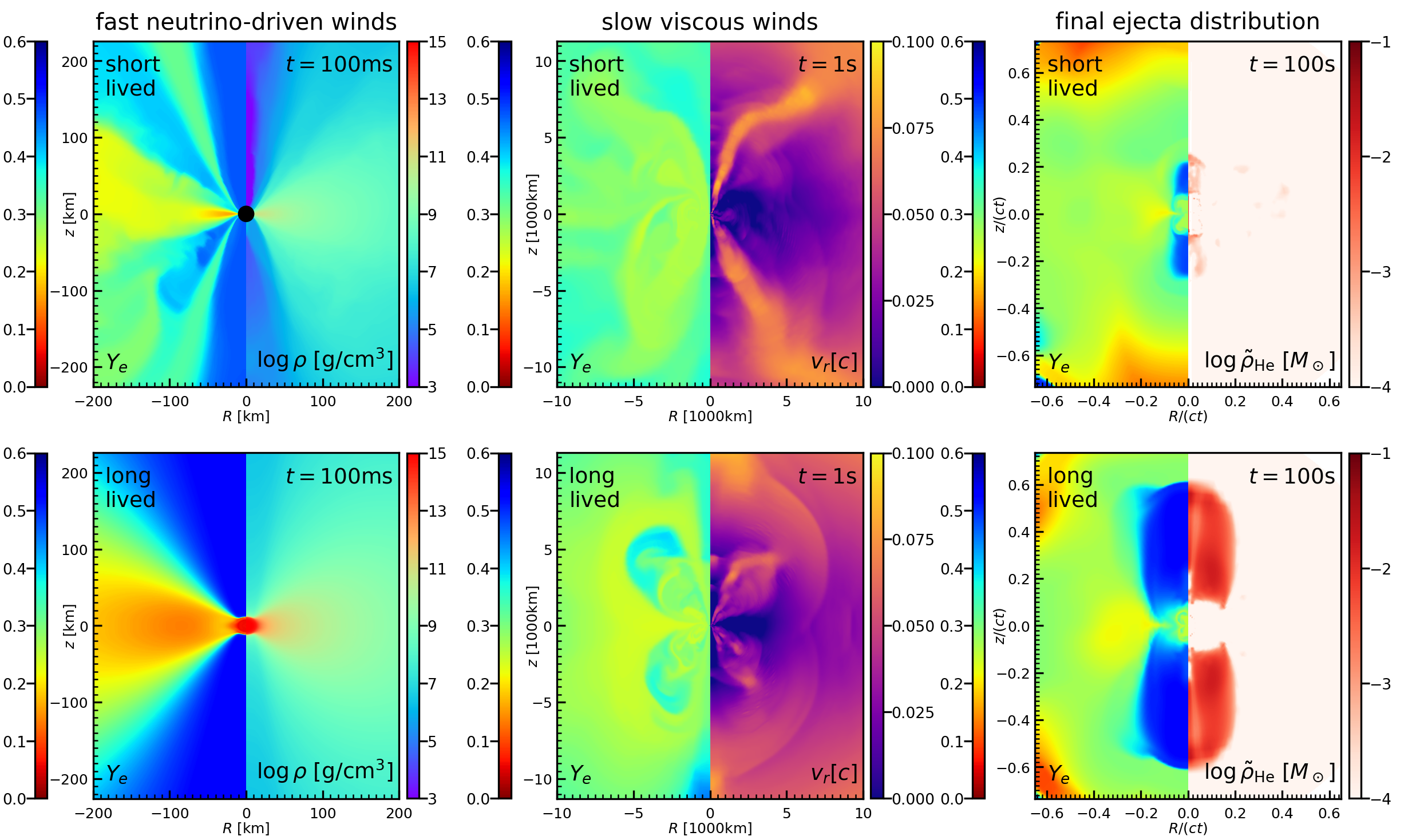
Figure 4: Snapshots from two numerical simulations in which the NS remnants are short lived (model “sym-n1-a6-short” with $\tau_{\mathrm{BH}}=10$ ms; top row) and long lived (“sym-n1-a6” with $\tau_{\mathrm{BH}}=122$ ms; bottom row) at three characteristic times after merger illustrating the launch of early, fast outflows (left column) and late, slow outflows (middle column) as well as the final ejecta configuration in velocity space (right column), where $Y_{e},\rho$, and $v_{r}$ are the electron fraction (measured before onset of the r-process), mass density, and radial velocity, respectively, and $\tilde{\rho}_{\mathrm{He}}=\mathrm{d}M_{\mathrm{He}}/\mathrm{d}\beta_{r}/\mathrm{d}\Omega=\rho X_{\mathrm{He}}\beta_{r}^{2}(ct)^{3}$ is the final helium density in dimensionless velocity space (with $\beta_{r}=r/(ct)$ and solid-angle element $\mathrm{d}\Omega$) rescaled by $\beta_{r}^{2}$ to enhance visibility for outflows with strong density decline. Being a stronger source of neutrinos than a BH-torus remnant, the NS remnant produces a far more massive and extended helium-rich, high-$Y_{e}$ ejecta component at early times, while the late BH-torus outflows are inefficient helium sources in both cases.

Helium is produced in nucleosynthesis conditions with high electron fractions, $Y_{e}\gtrsim 0.45$, and/or high entropies, $s\gtrsim 40\,{\rm k_{B}\,Baryon^{-1}}$, as highlighted in Fig. 3. The dynamical outflows expelled during the first $\sim 10\,$ms of NS mergers [95, 96, 97, 98, 99], as well as the viscous post-merger ejecta [100, 101, 102, 103, 104], typically show a broad pattern of conditions for $Y_{e}$ and $s$ with only a small fraction of material, if any, exhibiting sufficiently high values of either quantity to enable helium production. These ejecta components are therefore relatively inefficient sources of helium.

In contrast, high values of $Y_{e}$ and $s$ are characteristic of outflows powered by, or even just irradiated by, neutrinos. Neutrino-driven winds are well known from the field of core-collapse supernovae (CCSNe) [e.g. 105, 106, 107, 108, 109, 110, 111]. In such winds, material originating from high-density regions with strong electron degeneracy (and therefore typically low $Y_{e}$) is ejected as a consequence of continuous deposition of energy from absorption of neutrinos. The absorption reactions raise the entropy, lift the degeneracy, and increase the electron fraction of the ejecta.

An estimate of $Y_{e}$ resulting in neutrino winds can be obtained by neglecting neutrino emission and considering the equilibrium state achieved when the rates of $\nu_{e}$-absorption onto neutrons become equal to those of $\bar{\nu}_{e}$-absorption onto protons. This defines the value that $Y_{e}$ would relax to for given, fixed thermodynamic conditions and neutrino distributions. An estimate of this equilibrium value using the total number-loss rates, $L_{N,\nu}$, and typical mean-squared energies, $\langle\epsilon^{2}\rangle_{\nu}$, is given by [106, 112]:

$$Y_{e}^{\rm eq,abs}\approx\left(1+\frac{L_{N,\bar{\nu}_{e}}\langle\epsilon^{2}\rangle_{\bar{\nu}_{e}}}{L_{N,\nu_{e}}\langle\epsilon^{2}\rangle_{\nu_{e}}}\right)^{-1}\,.$$ (2)

Under quasi-stationary thermodynamic conditions the average $Y_{e}$ of the neutrino-emitting region changes only slowly, suggesting that equal numbers of $\nu_{e}$ and $\bar{\nu}_{e}$ are emitted per time, i.e. $L_{N,\bar{\nu}_{e}}\simeq L_{N,\bar{\nu}_{e}}$. Moreover, given that the (absorption and scattering) opacities of $\nu_{e}$ are comparable to those of $\bar{\nu}_{e}$, neutrinos of both species are emitted with similar spectra, i.e. $\langle\epsilon^{2}\rangle_{\nu_{e}}\simeq\langle\epsilon^{2}\rangle_{\bar{\nu}_{e}}$. For these reasons $Y_{e}^{\rm eq,abs}$ typically lies in a range close to 0.5 in neutrino winds. Considering that helium is produced very efficiently for $Y_{e}\gtrsim 0.45$ for a broad range of entropy conditions (cf. Fig. 3), this suggests neutrino winds to be suitable sites of helium production. However, Eq. 2 only provides a crude estimate of the actual $Y_{e}$, because it adopts a spherically symmetric field of free-streaming neutrinos, neglects the inverse (i.e. neutrino emission) processes, and assumes the absorption reactions to occur fast enough for $Y_{e}$ to reach the weak-equilibrium value. These assumptions are particularly problematic in NSMs, which due to the more complicated geometry compared to CCSNe produce more complex spatial distributions of neutrinos. Therefore, given the strong sensitivity of the helium yields on $Y_{e}$, hydrodynamic simulations need to be conducted with genuinely multi-dimensional neutrino-transport schemes capable of describing neutrino absorption in order to reliably predict helium yields in NSMs. An additional challenge, particularly for modeling the long-term evolution of merger remnants, is posed by the circumstance that small-scale turbulence, triggered primarily by the magneto-rotational instability [113], can have a substantial impact on the thermodynamic conditions and therefore the neutrino distributions and thus may, at least indirectly, affect the helium yields in neutrino winds from NSMs.

Due to their complexity, the properties of neutrino winds in NSMs are relatively poorly understood so far, despite a fair number of works devoted to their study [e.g. 114, 115, 116, 117, 118, 119, 101, 120, 121, 122, 123]. A characteristic tendency reported by many works adopting detailed neutrino schemes [e.g. 115, 119, 101, 124, 103, 125, 126] seems to be the stronger impact of neutrino irradiation near the poles compared to the equator, which results in particularly high $Y_{e}$ values and neutrino-heating rates along the polar directions. Neutrino winds can in principle be launched both before and after collapse of the NS remnant (which we denote as HMNS hereafter). However, since BH-tori are considerably weaker sources of neutrino emission than HMNSs, the neutrino-wind masses in BH-torus remnants are predicted to be much smaller than those of other ejecta components [100, 101, 127, 128]. Conversely, neutrino winds from the HMNS can be as massive as, if not more massive than, the dynamical and BH-torus ejecta [118, 121, 104], particularly when being enhanced due to magneto-hydrodynamic effects [129, 130, 49]. Thus, the ejecta launched during the HMNS phase are likely distinguished from the dynamical and BH-torus ejecta in that they produce a substantially greater amount of helium.

This notion is supported by our recent “end-to-end” neutrino-hydrodynamics simulations (see [121] and Appendix B for details) that describe all three evolutionary phases of matter ejection, namely the dynamical merger, the HMNS phase, and the final BH-torus evolution. In order to follow the properties of the neutrino wind as closely as possible, these models adopt a leakage scheme accounting for neutrino absoprtion [131] until 10 ms post merger and, subsequently, an energy-dependent two-moment transport scheme with a local closure (i.e. an M1 scheme; [132]). Angular-momentum transport due to small-scale turbulence is described using a recently developed two-parameter viscosity prescription inspired by the $\alpha$-viscosity scheme of Ref. [133]. The snapshots shown in Fig. 4 illustrate the crucial difference between a model with a short-lived HMNS remnant (with BH-formation time at $\tau_{\mathrm{BH}}\approx 10\,$ms, top row) and a long-lived one (with $\tau_{\mathrm{BH}}\approx 120\,$ms, bottom row): In the latter case the HMNS, due to its longer lifetime, gives rise to a massive and extended high-$Y_{e}$, high-entropy neutrino-driven wind along both polar directions, leading to substantial helium enrichment at final ejecta velocities of $0.15\lesssim v/c\lesssim 0.6$ within a cone of $\sim 20-40^{\circ}$ half-opening angle (see right panels of Fig. 4 for the spatial distribution of helium in the final ejecta configuration as well as Fig. A.4 for the mass distribution in $Y_{e}$ and $s$).

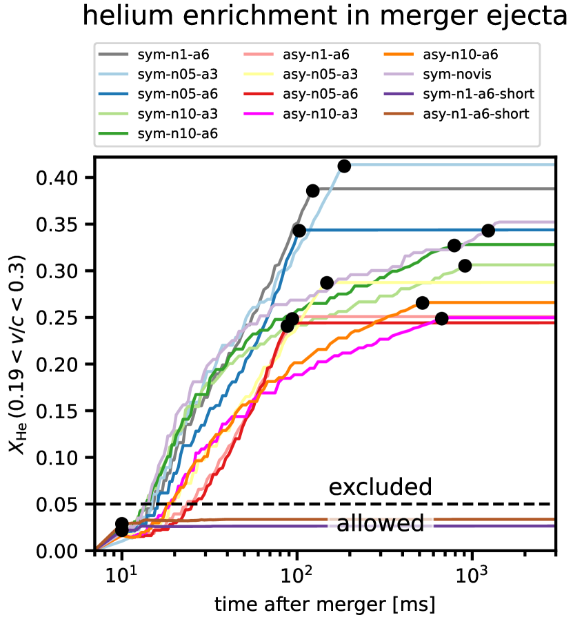
Figure 5: Mass of material ejected until the given time that will end up as helium relative to the mass of all material ejected until that time in our hydrodynamic simulation models (cf. Appendix B). Only material in the observationally relevant velocity range, $0.19<v/c<0.3$, is considered. We count as ejecta all material that at a given time lies beyond the radius of $50\,$km and is expanding faster than 0.1 $c$. The helium abundance plateaus following BH formation at $t=\tau_{\mathrm{BH}}$, indicated for each model with black circles. The observational constraint $X_{\mathrm{He}}=0.05$ is shown by the dashed line. Neutrino winds continuously inject helium into the ejecta but only as long as the HMNS is present, leading to a strong correlation between the helium abundance and the HMNS lifetime. In this set of models only the two short-lived models (denoted by “short” suffixes) with $\tau_{\mathrm{BH}}=10\,$ms satisfy the observational constraint.

Since the HMNS injects the wind with mass fluxes that vary only slowly with time, the relative fraction $X_{\mathrm{He}}(t)$ of mass ending up as helium in the observationally relevant (cf. Sect. II) velocity band $0.19\lesssim v/c\lesssim 0.3$ keeps growing continuously for the long-lived ($\tau_{\mathrm{BH}}>10\,$ms) models, reaching values of 20–40 $\%$ until abruptly saturating when the HMNS undergoes BH formation; see Fig. 5. Given a sufficiently long HMNS lifetime, helium becomes the most abundant element (by mass) in the entire outflow. Clearly, all the long-lived models shown in Fig. 5 are immediately ruled out by the observational constraint $X_{\mathrm{He}}<0.05$ (cf. Sect. II), while the short-lived models are compatible. Assuming that our set of models is representative concerning the behavior of $X_{\mathrm{He}}(t)$ (see discussion below), Fig. 5 implies that the observational constraint can only be fulfilled for relatively short lifetimes of

$$\tau_{\mathrm{BH}}\,(\,\mathrm{AT2017gfo}\,)\,\lesssim 20-30\,\mathrm{ms}\,.$$ (3)

In other words, the HMNS remnant in AT2017gfo must have collapsed within a few tens of milliseconds after the merger, because otherwise it would have blown out enough helium to be clearly observable in the kilonova spectra according to the P Cygni analysis of Sect. II. Importantly, given the rapid growth of $X_{\mathrm{He}}(t)$, even a less constraining bound, of say $X_{\mathrm{He}}<0.1$, would result in a strong lifetime constraint.

We note in passing that the large angular anisotropy created by the polar neutrino winds would also be at odds with the quasi-spherical geometry suggested by the observed spectral features in AT2017gfo (cf. for instance the P Cygni features and discussions in [85, 66], but see also [134]).

A few comments are in order regarding the lifetime constraint, Eq. 3. First, we stress that our set of models is still relatively small and therefore probably not exhaustive regarding the impact of different progenitor masses, mass ratios, EoSs, and turbulent viscosity prescriptions. However, the model-by-model variation of the time corresponding to $X_{\mathrm{He}}(t)=0.05$ is not more than about a factor of two, even for cases where the lifetimes $\tau_{\rm BH}$ differ by one order of magnitude, suggesting a certain robustness of the helium-enrichment mechanism and therefore a relatively mild sensitivity of the lifetime constraint, Eq. 3, with respect to these uncertainties. Considering specifically the viscosity, it is worth noting that the non-viscous model (sym-novis) exhibits the fastest rise of $X_{\mathrm{He}}(t)$ among all considered models, while a lifetime of $\tau_{\mathrm{BH}}\gtrsim 20\,$ms is only suggested by models with a relatively strong, and therefore possibly less realistic, viscosity.

An additional source of uncertainty is represented by the physics approximations adopted to make the simulations computationally feasible (concerning the treatment of general relativity, turbulent viscosity, and neutrino transport; see [121]). While the idea of HMNS remnants producing high-$Y_{e}$ winds is not new, the question of how fast these winds enrich the ejecta with helium is a difficult, quantitative question, sensitive to the detailed thermodynamic conditions and neutrino distribution near the HMNS surface, and to our knowledge this question has rarely been addressed so far (see, however, [74, 66] for studies discussing the impact of helium on kilonova spectra). Although our HMNS models capture more physics ingredients than many previous studies – in particular in that they adopt spectral neutrino transport – the remaining simplifying assumptions of our models may or may not have an impact on the $X_{\mathrm{He}}(t)$ curves. At any rate, the dichotomy between long-lived and short-lived models seen in Fig. 5 is striking, and we leave it to future work to explore in more detail the uncertainties of the $X_{\mathrm{He}}(t)$ dependence and of the implied lifetime constraint, Eq. 3.

A meaningful comparison with other literature results is difficult, if not impossible, at this point, because so far only a small number of merger-remnant simulations exist that are capable of describing neutrino winds combined with a (full or approximate) treatment of general relativistic gravity, while only a fraction of those report helium abundances, and none of them report helium abundances in just the relevant velocity band $0.19\lesssim v/c\lesssim 0.3$. We remark, however, that the results reported by Refs. [127, 122] for the neutrino wind of long-lived HMNSs appear to be in broad agreement with our models.

The polar nature of the helium-rich wind is particularly well suited for our observational constraint because of the near-polar viewing angle in AT2017gfo and the circumstance that absorption features in KN spectra are formed mainly along the line-of-sight. The broad velocity distribution of the wind, ranging from 0.1 $c$ to 0.6 $c$ is further auspicious for observability, because it safely encompasses the velocities of the line-forming region, $0.19c\lesssim v\lesssim 0.3c$, at around 4-5 days post merger. In earlier spectra, the observed line-forming region could constrain ejecta at larger velocities - even reaching out to $\sim$0.45$c$ at 1.17 days [66]. However, as deliberated in App. A.1, at earlier times radiative transitions will suppress the He i feature and imply weaker abundance constraints for such outer layers.

IV Equation of state constraints

IV.1 Lifetime

The upper limit on the remnant lifetime can be turned into an EoS constraint by recognizing that the lifetime indicates the proximity of the measured total binary mass, $M_{\mathrm{tot}}$, to the threshold mass for prompt black hole formation, $M_{\mathrm{thres}}$. The lifetime is expected to steeply decrease with higher total binary mass to reach roughly zero at $M_{\mathrm{thres}}$. In essence, therefore, the absence of significant amounts of He implies an upper limit on $M_{\mathrm{thres}}$. $M_{\mathrm{thres}}$ scales well with stellar parameters (e.g. radii, maximum mass, tidal deformability) of non-rotating NSs [136, 137, 138, 35, 139, 140, 39, 141, 142, 143, 144], which can thus be constrained. This line of argument has already been presented in [33] (see Fig. 5 in that paper for a hypothetical case).

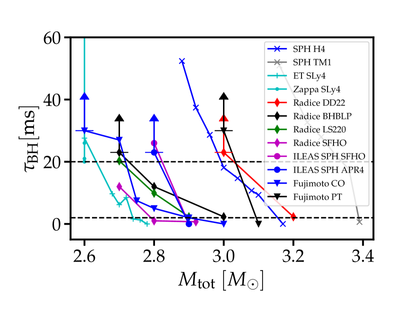
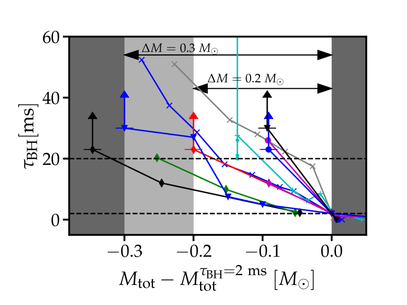
Figure 6: Upper panel: Remnant lifetimes in sequences of simulations of equal-mass mergers varying only the total binary mass $M_{\mathrm{tot}}$. Colors and symbols refer to different EoS and simulation tools, respectively. From the literature we adopt data from [34, 145, 146] (from [145] we only include calculations at a fixed binary mass for different simulation settings to indicate uncertainties). Dashed lines indicating life times of 2 ms and 20 ms are drawn to estimate $\Delta M=M_{\mathrm{thres}}-M_{\mathrm{tot}}^{\tau_{\mathrm{BH}}=20\,\mathrm{ms}}$ for the various EoS models. Arrows display lower limits on $\tau_{\rm BH}$, where $\tau_{\rm BH}$ is given by the end of the simulation time, until which no gravitational collapse took place. Lower panel: Same sequences as in the upper panel but shifted by $-M_{\mathrm{tot}}^{\tau_{\mathrm{BH}}=2\,\mathrm{ms}}$ to read off an estimate of $\Delta M$.

In a first step, we thus consider the dependence $\tau_{\mathrm{BH}}(M_{\mathrm{tot}})$, where one expects that the lifetime decreases with $M_{\mathrm{tot}}$ since more mass destabilizes the remnant (e.g. [147]). The loss and redistribution of energy and angular momentum of the central object are governed by the magneto-hydrodynamical evolution, gravitational-wave emission and neutrino emission. For higher binary masses these processes take less time to drive the remnant to a more compact and ultimately unstable configuration. The exact dependence of the lifetime on the binary masses is notoriously difficult to determine because the remnant lifetime in numerical simulations is strongly affected by numerics, e.g. the numerical resolution, discretization schemes or the choice of the initial orbital separation, and the physics included (e.g. neutrinos, magnetic fields or effective viscosity) [145, 138]. In addition, $\tau_{\mathrm{BH}}(M_{\mathrm{tot}})$ may not even be unique for a given numerical scheme and input physics but be to a certain extent subject to stochastic simulation-to-simulation variations. One should also expect a dependence on the EoS and the binary mass ratio as well. Surveying the literature there are hardly any studies available that explicitly determine $\tau_{\mathrm{BH}}(M_{\mathrm{tot}})$ by running sequences of models with fine spacing in $M_{\mathrm{tot}}$ within the range of interest (0 ms $\lesssim\tau_{\mathrm{BH}}\lesssim 40$ ms) based on a set of consistent simulations (i.e. with calculations varying only $M_{\mathrm{tot}}$ but otherwise using the same numerical and physical setup), which is essential to obtain values that can be meaningfully compared (but see Lucca and Sagunski [148], Holmbeck et al. [59] for a meta-study, which however does not include sufficiently fine spaced model setups within a consistent treatment; and see discussion and Fig. 6 in Kölsch et al. [138], which includes $q<1$ cases). For the sake of our argument, however, a coarse estimate suffices taking advantage of the fact that $\tau_{\mathrm{BH}}(M_{\mathrm{tot}})$ is likely a very steep function (as suggested by simulations). We intend to estimate an upper limit on $\Delta M$ being the difference between $M_{\mathrm{thres}}$ and the measured binary mass of GW170817.

In Fig. 6 we collect data from different simulations showing the lifetime as a function of the total binary mass for equal-mass binaries. This includes different calculations with our smoothed-particle hydrodynamics (SPH) code employing the conformal flatness approximation as in [149, 150]. The runs labelled “ILEAS SPH” incorporate a account for neutrino emission effects [131]. We also include runs with the Einstein Toolkit [151] in full general relativity as in [152] but for the Sly4 EoS [153] and a set of simulations from the literature in full GR partly in combination with a neutrino treatment [34, 146]. For the latter, the simulation setups are coarsely spaced in $M_{\mathrm{tot}}$. To indicate uncertainties we add calculations for a fixed binary mass and EoS, but with different numerical resolution, neutrino treatment and partly a scheme to model turbulent viscosity from Zappa et al. [145]. For clarity we drop some data points with a prompt collapse, which presumably have a total binary mass much in excess of $M_{\mathrm{thres}}$. There are different definitions of a prompt collapse and of $M_{\mathrm{thres}}$ discussed in the literature [35, 138, 143]. To estimate $\Delta M=M_{\mathrm{thres}}-M_{\mathrm{tot}}$, we adopt the notion of Agathos et al. [139] and Kölsch et al. [138], defining $M_{\mathrm{thres}}$ as the system with $\tau_{\rm BH}$ $=2$ ms. In Fig. 6 the dashed horizontal lines indicate life times of 2 ms and 20 ms. Reading off $\Delta M$ by the intersections of the respective curves for the various EoSs at 2 ms and 20 ms, we find values in the range between 0.048 M_⊙ and 0.319 M_⊙ with only two out of the eleven EoSs exceeding 0.2 M_⊙ (see lower panel in Fig. 6). We stress again that these values are only tentative because of the limited number of sequences, the, in places, coarse sampling in $M_{\mathrm{tot}}$ and our poor knowledge of underlying (numerical or physical) uncertainties.

The sparseness of the current data prevents us from estimating $\Delta M$ for a limit of $\tau_{\rm BH}$ $=30$ ms or even $\tau_{\rm BH}$ $=40$ ms, but $\tau_{\mathrm{BH}}(M_{\mathrm{tot}})$ typically becomes steeper in this range (as indicated in the figure) and thus $\Delta M$ should not be much affected by the exact limit on $\tau_{\rm BH}$ implied by the observed lack of helium.

For the following derivation of the EoS constraints we therefore adopt $\Delta M=0.2$ M_⊙ as a sensible choice and we present results for $\Delta M=0.3$ M_⊙ and $\Delta M=0.4$ M_⊙ as a more conservative approach in App. C. We note that Fig. 6 of [138] indicates a similar range of $\Delta M\approx 0.2$ M_⊙ (also for asymmetric binaries). A value of $\Delta M=0.2$ M_⊙ implies that for the measured binary mass of $M_{\mathrm{tot}}^{\mathrm{GW170817}}=2.73^{+0.04}_{-0.01}$ M_⊙ [9], the threshold mass for prompt gravitational collapse is unlikely to exceed $2.93^{+0.04}_{-0.01}$ M_⊙.

IV.2 Constraints on stellar parameters: radius, tidal deformability and maximum mass

An upper limit on the threshold mass implies constraints on NS radii and the maximum mass of non-rotating NSs, $M_{\mathrm{max}}$, because $M_{\mathrm{thres}}$ scales tightly with these properties [136, 137, 138, 35, 139, 140, 39, 141, 142, 143, 144]. Generally, the threshold mass increases with $M_{\mathrm{max}}$ and NS radius, $R$, (or equivalently the tidal deformability, $\Lambda$). Consequently, both quantities, $M_{\mathrm{max}}$ and $R$, cannot simultaneously become too large to accommodate a given upper limit on $M_{\mathrm{thres}}$. Furthermore, $M_{\mathrm{thres}}$ depends on the binary mass ratio $q$ [140, 39, 144, 138]. A number of fit formulae for $M_{\mathrm{thres}}$ have been developed describing these dependencies based on the analysis of a large set of numerical simulations determining $M_{\mathrm{thres}}$ for different EoS models and mass ratios [39, 138]. The exact fit formulae and their tightness are affected by the number and type of considered EoS models, the binary mass ratio, and the numerical tool.

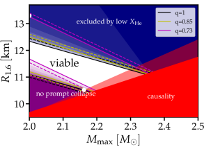
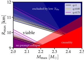
Figure 7: Constraints on the radius of a 1.6 M_⊙ NS (left) and the radius, $R_{\mathrm{max}}$, of the maximum-mass configuration (right) as function of maximum mass $M_{\mathrm{max}}$. Stellar parameters in the upper right corner (blue area) are ruled out for a total binary mass $\sim 0.2\,$M_⊙ below the threshold mass for prompt black-hole formation $M_{\mathrm{thres}}$. This binary mass is derived from the maximum lifetime of $\sim$20 ms inferred for the merger remnant from the absence of strong He features in the kilonova spectrum, as explained in the text. Small NS radii in the lower left are excluded if GW170817 did not undergo a prompt gravitational collapse (as argued in [33, 39]) based on the high kilonova brightness (purple area). Solid lines in the respective regions display constraints for assumed binary mass ratios of $q=1$ (black), $q=0.85$ (yellow) and $q=0.73$ (magenta). Dashed lines of the same color include additionally the uncertainty from the scatter in the fit formula for $M_{\mathrm{thres}}(q,M_{\mathrm{max}},R)$. The color shading of the blue and purple area indicates confidence levels of exclusion (in 10% steps) from considering the posterior distribution of the binary mass ratio of GW170817. Shading for the area between the 0% and 10% levels are not plotted. For the upper limit, note the initial steep increase with the 50% level close to the yellow line ($q=0.85$). For the lower limit, the confidence of exclusion drops steeply between the 90% level (close to the black solid line for $q=1$) and the 50% level (close to the yellow solid line for $q=0.85$). Causality excludes the dark red region. Stellar parameters in the light red area are empirically not found in a large set of microphysical EoS models. White dots in the left panel show absolute limits at the 90% confidence level given by $M_{\mathrm{max}}=2.0\,$M_⊙ for the upper limit and the intersection with the empirical exclusion region (light red area) for the lower limit. These dots show the $R_{1.6}$ constraints visualized in Fig. 9. See main text for more information.

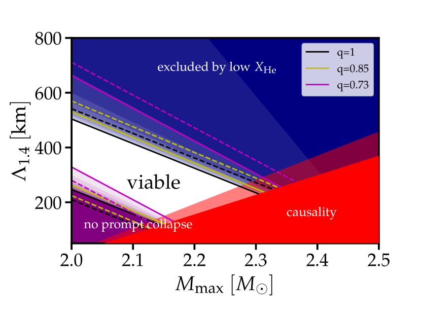
Figure 8: Same as Fig. 7 but for the tidal deformability $\Lambda_{1.4}$ of a 1.4 M_⊙ NS.

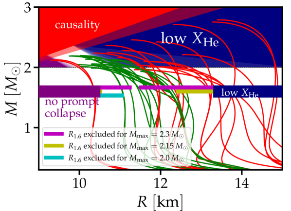
Figure 9: Constraints on NS parameters as in Fig. 7 overplotted with exemplary mass-radius relations for various microphysical EoSs (green and red lines) [154, 155, 156, 157, 158, 159, 160, 161, 162, 163, 164, 165, 166, 153, 167, 168, 169, 170, 169, 171, 172, 173, 174, 175, 176, 177, 36, 178, 179, 180, 181, 182]. If the remnant of GW170817 was short-lived, this excludes stellar parameters in the blue areas (see main text). NS radii are constrained from below (purple areas) because the brightness of the kilonova AT2017gfo points to no prompt collapse yielding a lower limit on $M_{\mathrm{thres}}$. The color shadings of the constraints on $\{M_{\mathrm{max}},R_{\mathrm{max}}\}$ above $M=2.0\,$M_⊙ (thin dashed horizontal line) resemble the exclusion probability implied by the posterior distribution of the binary mass ratio in GW170817 [9] similarly as in Figs. 7 and 8. Causality rules out the area in the upper left corner. Note that a mass-radius curve is only excluded if its $\{M_{\mathrm{max}},R_{\mathrm{max}}\}$ lies in one of the excluded regions. The horizontal bars around $M=1.6\,$M_⊙ display the upper and lower limit on $R_{1.6}$ with the purple and blue areas providing the absolute limits independent of $M_{\mathrm{max}}$ (at 90% confidence based on the binary mass ratio distribution; see black dots in left panel of Fig. 7 and main text). The magenta, yellow and cyan bars give the bounds for specific values of $M_{\mathrm{max}}$. For $M_{\mathrm{max}}\gtrsim 2.15~{}M_{\odot}$ the causality or empirical limit, respectively, become more stringent then the lower bound from the “no prompt collapse” argument and the allowed range of $R_{1.6}$ becomes increasingly smaller approaching zero for $M_{\mathrm{max}}\approx 2.3~{}M_{\odot}$ and thus EoSs with $M_{\mathrm{max}}\gtrsim 2.3~{}M_{\odot}$ are ruled out. Mass-radius relations shown in red are excluded by our constraints. See main text for more detailed explanations.

For our constraint we employ the fit formulae from Ref. [39], which simultaneously include a dependence on the EoS and $q$ for a very large number of EoSs (more than 20 models). We note that the influence of the binary mass ratio turns out to be considerable, which is why it is important to use a fit that equally covers the EoS and mass ratio dependence. We adopt the prescription

$$M_{\mathrm{thres}}(q,M_{\mathrm{max}},R)=c_{1}M_{\mathrm{max}}+c_{2}R+c_{3}+c_{4}\delta q^{3}M_{\mathrm{max}}+c_{5}\delta q^{3}R$$ (4)

from [39] with fit parameters $c_{i}$ and $\delta q\equiv 1-q$. The radius $R$ may be the radius $R_{1.6}$ of a 1.6 M_⊙ NS or the radius $R_{\mathrm{max}}$ of the maximum mass configuration. $R$ may also be replaced by the tidal deformability of a NS with fixed mass, e.g. 1.4 M_⊙. See Tab. VI in [39] for the fit parameters $c_{i}$ resulting from different underlying datasets; we choose the fits for the EoS sample ‘b’, i.e. the subset of purely baryonic EoS models which are compatible with pulsar observations [183, 184, 185] and the tidal deformability from GW170817 [9] (see App. C for further comments on the choice of the fit formula; for convenience Tab. 1 lists coefficients of all relations employed in this study).

For $M_{\mathrm{thres}}\leq M_{\mathrm{tot}}^{\mathrm{GW170817}}+\Delta M$, it immediately follows that

$$R\leq\frac{M_{\mathrm{tot}}^{\mathrm{GW170817}}+\Delta M-c_{1}M_{\mathrm{max}}-c_{3}-c_{4}\delta q^{3}M_{\mathrm{max}}}{c_{2}+c_{5}\delta q^{3}},$$ (5)

where $\Delta M$ can be further increased to include additional sources of error, e.g. the tightness $\delta M$ of the fit formulae. We display the constraint on $R_{1.6}$ resulting from Eq. (5) in Fig. 7 (blue area in the upper right in the left panel). In Fig. 7 the lines refer to fixed binary mass ratios adopted in Eq. (5). In Eq. (5) we include the total binary mass of GW170817 using the well measured chirp mass $\mathcal{M}$ via $M_{\mathrm{tot}}=\mathcal{M}q^{-3/5}(1+q)^{6/5}$. Dashed lines indicate the constraints for fixed mass ratios adding the mean deviation $\delta M=0.017\,$M_⊙ of the fit from the underlying data as additional error to $\Delta M$ (see eighth column in Tab. VI for $\delta M$ in [39]).

In GW170817, the binary mass ratio was found to be in the range $0.73\leq q\leq 1$ at the 90% confidence level assuming a low spin prior [9]. Figure 7 shows a strong dependence on the binary mass ratio with $q=0.73$ yielding the weakest constraint unless $M_{\mathrm{max}}\gtrapprox 2.3\,$M_⊙. Equation (5) shows a complicated behavior with $q$ depending on the chosen $M_{\mathrm{max}}$, which for intermediate $M_{\mathrm{max}}$ can even be non-monotonous. For smaller $M_{\mathrm{max}}$, the maximum allowed radius is increasing with the binary mass asymmetry in Eq. (5). The posterior probability of $q$ from GW170817 shows a relatively flat distribution for $0.8\lesssim q\lesssim 1$ to decrease more steeply below $\sim 0.8$ (see Fig. 7 in [9]). Thus, it is statistically very unlikely that the mass ratio was in the range $q\lesssim 0.7$. Using the posterior distribution of $q$ from Ref. [9], we use ten different shadings to indicate the exclusion levels in Fig. 7 in 10% steps resulting from the distribution of $q$, which we propagate through Eq. (5).

Note that the dependence on $q$ in Eq. (5) is such that stronger deviations from the $q=1$ case only occur for very asymmetric systems because of the $\delta q^{3}$ terms in Eq. (4). The line for $q=0.85$ (yellow) is very close to that of the equal-mass mergers (black) in Fig. 7. Thus the probability that a radius is excluded rises quickly in the region between the lines with $q=1$ and $q=0.85$ (different shadings are hardly distinguishable in this range in Fig. 7). The 50% exclusion contour is very close to the $q=0.85$ line (yellow); the 90% limit follows closely the $q=0.73$ line (magenta) for $M_{\mathrm{max}}\lesssim 2.4\,$M_⊙.

Large radii cannot be ruled out if GW170817 was very asymmetric. The reason for this lies in the behavior of $M_{\mathrm{thres}}(q)$, which is relatively flat for small binary mass asymmetries ($q\approx 1$) and declines stronger for larger asymmetries, i.e. smaller $q$ (see e.g. Fig. 4 in [39] or [140, 144, 138]). Even a stiff EoS could thus yield a relatively small $M_{\mathrm{thres}}$ if the binary was very asymmetric implying only a weak constraint on the radius. In addition, significant binary mass asymmetries imply a higher total binary mass of GW170817, for which only the chirp mass is well known, and thus weaken our upper radius limit.

We note that the fit formulae do not consider intrinsic spins of the NSs, which however affect $M_{\mathrm{thres}}$ only for very large and probably unrealistic values [141, 186]. We show the impact of strong first-order phase transitions on our constraints in App. C and find that they would weaken the radius constraints by a few hundred meters if $M_{\mathrm{max}}\sim 2\,$M_⊙ and if phase transitions are as extreme as the ones adopted in [39]. We also present the limits resulting from alternative fit formulae [138] in the appendix, which only mildly affect the quantitative results. Thus the main uncertainty still remains that of the binary mass ratio.

As already apparent from Eq. (5), the new upper limit on $R_{1.6}$ depends on the maximum mass and becomes stronger for larger $M_{\mathrm{max}}$. This is clear because $R$ and $M_{\mathrm{max}}$ both increase $M_{\mathrm{thres}}$ (cf. Eq. (4)), and a larger $M_{\mathrm{max}}$ is only compatible with $M_{\mathrm{thres}}\lesssim 2.9\,$M_⊙ if the radius is correspondingly smaller. The fact that our limits depend on $M_{\mathrm{max}}$ make them more constraining than an individual number suggests: large radii are only compatible with relatively small $M_{\mathrm{max}}$ – just above the current lower bound [183, 184, 185]. This is rather atypical for many EoS models, which often reach far beyond 2 M_⊙ if the radius $R_{1.6}$ is larger than $\sim 12$ km. Our constraint thus rules out a significant number of current EoS models, which can be directly seen in Fig. A.5, where the stellar parameters of a sample of microphysical EoS models are overplotted.

We include two additional constraints in Fig. 7. In the lower left part we display the excluded region (purple) derived from the argument that GW170817 was likely not a prompt collapse event, which would be incompatible with the relatively high brightness of the kilonova [33]. A prompt collapse is likely connected with reduced mass ejection and, thus, one concludes that $M_{\mathrm{thres}}>M_{\mathrm{tot}}^{GW170817}$. Following [33, 39], this implies a lower limit on the radius. We update and improve this constraint in comparison to [33, 39] by employing for consistency the same $q$-dependent fit formula for $M_{\mathrm{thres}}$ (Eq. (4)) and by considering the posterior sample of $q$ from GW170817. Instead of only computing an absolute lower limit as in [39] we show the lower limit as function of $M_{\mathrm{max}}$. As for the upper limit, the lower limits directly result from Eq. (4) as

$$R>\frac{M_{\mathrm{tot}}^{\mathrm{GW170817}}-c_{1}M_{\mathrm{max}}-c_{3}-c_{4}\delta q^{3}M_{\mathrm{max}}}{c_{2}+c_{5}\delta q^{3}}.$$ (6)

Again we find a significant impact from the binary mass ratio especially for $M_{\mathrm{max}}\approx 2\,$M_⊙. This can be seen from the lines in the lower left of the figure, where in contrast to the upper limit the $q=1$ case represents the more conservative limit. The dashed lines again indicate the uncertainties of the fit formula (by shifting $M_{\mathrm{tot}}^{\mathrm{GW170817}}\rightarrow M_{\mathrm{tot}}^{\mathrm{GW170817}}-\delta M$ in Eq. (6)). We again propagate the posterior sample of $q$ from GW170817 through Eq. (6) and use different shadings in Fig. 7 to visualize the exclusion level in steps of 10% (purple area). As for the upper limit the resulting distribution becomes very steep in the range corresponding to small binary mass asymmetries. The 90% level is close to the black solid line ($q=1$) and the 50% level follows closely the yellow $q=0.85$ line.

Like the upper limit, the lower limit on the radius also depends on the maximum mass and effectively the combined constraint appears like a “sliding window”, where larger radii are favored for relatively small maximum masses $\sim 2\,$M_⊙ and smaller radii are only compatible with larger $M_{\mathrm{max}}$. The sliding window essentially is a result of our main argument that $M_{\mathrm{tot}}^{\mathrm{GW170817}}<M_{\mathrm{thres}}\leq M_{\mathrm{tot}}^{\mathrm{GW170817}}+\Delta M$. Recall that the lower limits are independent of $\Delta M$ and the presence or absence of helium, and $\Delta M$ determines the width of the allowed range in $R_{1.6}$.

The second additional constraint we consider arises because causality limits the stiffness of any EoS. In the lower right of Fig. 7 (left panel) we display an area which is excluded by causality requiring that the speed of sound $v_{s}$ cannot exceed the speed of light $c$. This limits the maximum stiffness of the EoS and consequently rules out large $M_{\mathrm{max}}$ for a given $R_{1.6}$. Being less conservative, we obtain an “empirical” limit by considering pairs $\{R_{1.6},M_{\mathrm{max}}\}$ from a large set of microphysical EoSs and determining the limit such that all models lie within this phenomenological bound. See [33, 36, 39] and App. C for the details on the “causality limit” and the “empirical limit”.

One may expect that an upper limit on $M_{\mathrm{thres}}$ also implies a constraint on $M_{\mathrm{max}}$. This constraint is visible in Fig. 7, where the intersection between the empirical or causal limit (red area) and the upper limit on $R_{1.6}$ (blue area) provides the highest possible $M_{\mathrm{max}}$. Based on the argument of a low helium mass fraction, we can rule out $M_{\mathrm{max}}\gtrsim 2.3$ M_⊙ for $\Delta M=0.2\,$M_⊙. We emphasize that large $M_{\mathrm{max}}$ far in excess of 2 M_⊙ are only compatible with a relatively narrow range of radii because for $M_{\mathrm{max}}\gtrsim 2.15\,$M_⊙ the phenomenological and causality constraints become stronger than the bound from the no-prompt-collapse argument. This significantly tightens the “allowed window” in this $M_{\mathrm{max}}$ range. Note that the numbers for the lower radius limit derived in [33, 39] (i.e. $\sim 10.5$ km) essentially correspond to the point where the lines of the lower limit (cf. Eq. (6)) intersect with the empirical or causality constraint (red area). This represents a more conservative limit independent of $M_{\mathrm{max}}$ and provides an absolute lower bound. Table 2 lists the absolute upper limits on $M_{\mathrm{max}}$, which range from about 2.3 M_⊙ to 2.5 M_⊙ depending on $\Delta M$, and the absolute lower and upper limits on NS radii.

In Fig. 7 (right panel) we visualize the constraint on the radius $R_{\mathrm{max}}$ of the maximum mass configuration employing a fit formula $M_{\mathrm{thres}}(q,M_{\mathrm{max}},R_{\mathrm{max}})$ but otherwise following the same line of argument and derivation (fit for set ‘b’ in Tab. VI in [39]). For the dark red exclusion region (from causality arguments) we use results from Refs. [187, 4], whereas the corresponding empirical limit (light shading) is again obtained from considering a large set of microphysical EoS models (see App. C, Tab. 2).

Figure 8 shows the constraints on the tidal deformability $\Lambda_{1.4}=\Lambda(1.4~{}M_{\odot})$ (fit for set ‘b’ in Tab. VI in [39]). The excluded area in the lower right (red) is obtained in a way equivalent to the corresponding constraint on $R_{1.6}$ (see App. C).

We summarize the various constraints on NS radii in Fig. 9 in comparison to a set of different microphysical EoSs (same sample as in [39]). For the maximum-mass configurations, we display the constraints on $\{M_{\mathrm{max}},R_{\mathrm{max}}\}$ (in the upper part of the diagram) with the shading reproducing the likelihood of different binary mass ratios of GW170817 as in Fig. 7. A mass-radius relation of an EoS can cross this exclusion region and the model remains still viable if $\{M_{\mathrm{max}},R_{\mathrm{max}}\}$ lie in the allowed region.

The exact constraints on $R_{1.6}$ are not straightforward to visualize in Fig. 9 because they depend on $M_{\mathrm{max}}$. As discussed above the position of the “allowed” window shifts with $M_{\mathrm{max}}$ but its width is approximately constant for $M_{\mathrm{max}}\lesssim 2.15\,$M_⊙. For $M_{\mathrm{max}}\gtrsim 2.15\,$M_⊙ the allowed range of $R_{1.6}$ becomes increasingly smaller (see left panel of Fig. 7). For $M_{\mathrm{max}}\approx 2.3~{}M_{\odot}$ this range decreases to zero and models with $M_{\mathrm{max}}\gtrsim 2.3\,M_{\odot}$ are excluded. The wide purple and blue bars at $M\approx 1.6~{}M_{\odot}$ display the 90% exclusion limits for a respective absolute limit independent of $M_{\mathrm{max}}$. For the upper bound the absolute limit is given by the constraint for $M_{\mathrm{max}}=2.0\,$M_⊙, whereas the absolute lower bound results from $M_{\mathrm{max}}=2.126\,$M_⊙ (see markers in left panel of Fig. 7). We stress that for any other $M_{\mathrm{max}}$ the limits are more stringent, which is illustrated by the magenta, yellow and cyan bars showing the corresponding bounds on $R_{1.6}$ for specific values of $M_{\mathrm{max}}$ in Fig. 9 (adopting the 90% limits from the posterior distribution of the binary mass ratio). Thus, the absolute limits (wide blue and purple bars) do not adequately represent the constraining power of our constraints on $R_{1.6}$. For instance, a $M-R$ curve passing close to the blue region at $M=1.6$ M_⊙ (“no He” constraint) cannot reach much higher than 2 M_⊙. Hence, some of the shown models compatible with $R<13.29$ km (blue) are in fact excluded. Larger $M_{\mathrm{max}}$ are only compatible with smaller $R_{1.6}$. Similarly, if an $M-R$ relation passes close to the purple exclusion region (“no prompt collapse” constraint), its maximum mass should be relatively large and an EoS model with $M_{\mathrm{max}}\approx 2.0\,$M_⊙ would be excluded.

The resulting constraints on the stellar properties of NSs for adopting $\Delta M=0.3\,$M_⊙ or even $\Delta M=0.4\,$M_⊙ are provided in App. C. We stress that a chosen $\Delta M$ is equivalent to adopting an upper bound on $M_{\mathrm{thres}}=M_{\mathrm{tot}}^{\mathrm{GW170817}}+\Delta M$. This implies that the upper limits discussed in our study would generally result from any upper bound on the threshold mass for prompt black hole formation, which may be inferred in the future. Thus our constraints on stellar parameters for different $\Delta M$ will be directly applicable to any upcoming upper limit on $M_{\mathrm{thres}}$.

Considering Eqs. (5) and (6) it is clear how future NSM observations may further improve the constraints presented here. As already argued in [33, 39], a bright kilonova with a higher chirp mass would imply a stronger constraint on the lower limit of $R$ (or $\Lambda$). As apparent from the figures, an event with the same chirp mass but a well measured binary mass ratio $q<1$ would, if a prompt collapse could be excluded, as in GW170817, shift the lower bound to larger radii. Similarly, a GW170817-like detection but with well-measured $q\approx 1$ would imply a decrease of the upper limit on $R$ or $\Lambda$ and mean a stronger EoS constraint. Also, if a new detection with lower chirp mass showed no signs of a significant helium enrichment, the upper bounds on $R$ or $\Lambda$ would be shifted to smaller values and the upper limit on $M_{\mathrm{max}}$ strengthened as well. We finally remark that the (absolute) upper limit on $R$ or $\Lambda$ obviously depends on the lower bound on $M_{\mathrm{max}}$, which is given by the most massive NS mass measurement (for simplicity we adopt a value of 2 M_⊙ consistent with [183, 184, 185]). Clearly, a well-determined lower bound on $M_{\mathrm{max}}$ with a greater value would further improve our radius constraint.

V Further implications

If AT2017gfo indeed harbored a short-lived HMNS remnant, as we argue here, this would have several further interesting implications.

V.1 Magnetar-powered short GRBs?

GW170817 was accompanied by an sGRB (GRB170817A), presumably powered by a highly-relativistic jet outflow launched in the aftermath of the merger. A short HMNS lifetime of just a few tens of milliseconds renders the magnetar scenario (e.g. [48, 49]) for launching this jet very unlikely in this system. It strongly supports the BH-torus scenario, i.e. the jet was probably powered by the Blandford-Znajek process [188] (or possibly by neutrino-pair annihilation [189] or a combination of both, though neutrino-pair annihilation is less favored given its relatively low efficiency [190]). Assuming further that the binary system in GW170817 is representative of NS binaries, then most observed sGRBs would be powered by BH-torus central engines.

V.2 GW190814 interpretation

The nature of the secondary compact object in the gravitational-wave event GW190814 [191] with a mass of $2.5$-$2.67\,M_{\odot}$ is not safely identified so far. While a BH seems to be likely [e.g. 192, 193], a NS cannot be completely ruled out at present [e.g. 194]. The upper limit for the maximum NS mass presented here, i.e. $M_{\rm max}<2.3\,M_{\odot}$, would exclude a NS interpretation unless the secondary was rapidly spinning, which implies the secondary to be the lightest BH ever discovered. This conclusion even holds for the very conservative assumption of $\Delta M=0.4\,M_{\odot}$.

V.3 Predictions for future observations

If the total mass $M_{\mathrm{tot}}^{\mathrm{GW170817}}$ in GW170817 was indeed relatively close to the threshold mass for prompt collapse, then NSMs with somewhat higher total masses than that of GW170817 would lead to prompt BH formation. This implies that for future observations of such events with $M_{\mathrm{tot}}>M_{\mathrm{tot}}^{\mathrm{GW170817}}+\Delta M$ no gravitational-wave signal from the oscillating NS remnant will be detectable even for nearby events and the kilonova would be expected to be significantly fainter than AT2017gfo because of a smaller ejecta mass. We would also infer that any system more massive than GW170817 should also not exhibit a strong spectral signature of helium (unless GW170817 was very asymmetric, in which case a more massive equal-mass system might yield a longer lifetime). If the merger outcome can be unambiguously identified, for instance through the kilonova brightness or the post-merger GW signal, our prediction of a prompt-collapse event for binary masses close to $M_{\mathrm{tot}}^{\mathrm{GW170817}}+\Delta M\approx 2.9\,$M_⊙, which is relatively low compared to most predicted $M_{\mathrm{thres}}$ (see e.g. Tab. IX in [39]), can be seen as a strong test of the arguments laid out in this paper.

On the other hand, in future events with a smaller total mass than GW170817 and consequently $\tau_{\rm BH}$ in the several tens, hundreds or thousands of milliseconds, a helium feature should be present for a polar observer in late photospheric epochs, due to the longer lifetime and correspondingly higher neutrino-wind masses. Specifically, we predict this to be the case for binary masses below a certain critical mass $M_{\mathrm{tot}}^{\mathrm{He}}$ with $M_{\mathrm{tot}}^{\mathrm{GW170817}}-\Delta M<M_{\mathrm{tot}}^{\mathrm{He}}<M_{\mathrm{tot}}^{\mathrm{GW170817}}$, where the exact value depends on how close $M_{\mathrm{tot}}^{\mathrm{GW170817}}$ was to $M_{\mathrm{thres}}$. A clear helium spectral feature may point to a longer lifetime than in GW170817 assuming the ejecta properties (e.g. electron densities and deposition rates) to be similar to those of GW170817. In the event of a NSM detection with a nearly identical total mass to GW170817, a strong helium spectral feature may point to a longer lifetime than in GW170817. This could be explained by a more symmetric progenitor mass configuration ($q$ closer to unity) compared to GW170817, as stability of the remnant typically decreases with smaller mass ratios [140, 39, 138, 144].

Future detections of kilonovae and sGRBs could also be made without detecting the GW signal, i.e. lacking information on the mass of the binary (e.g. GRB 211211A [195, 196] and GRB 230307A [60]). In such “orphan-kilonova” cases, the appearance or absence of a helium feature in the observed kilonova spectra at a constraining epoch may provide an indication of the mass relative to GW170817.

The helium constraints proposed in this paper can be tested if future observations can reveal the remnant lifetime independently, e.g. through the shut-off of the post-merger GW signal [197, 198] or the ringdown of the newly formed BH [199] or, possibly, through extended X-ray emission found in a subset of observed sGRBs [e.g. 200, 201, 202]. Such a direct detection through the GW signal requires a high signal-to-noise ratio, however, and will only be possible for a very close event and/or with next-generation GW detectors (such as the Einstein telescope [203]).

V.4 Improved He abundance measurement by modeling of Sr ii

The helium upper limits in this analysis are reached assuming negligible contribution from the Sr ii lines, which are known to be a significant and dominant contributor to the feature in all earlier epochs [61, 63, 69, 204, 65, 66]. It is likely that the relevant Sr ii lines contribute to, and probably dominate, the feature at 4.4 days, which implies that the corresponding contribution from He i $\lambda 1083.3$ nm is even lower than presented here. More constraining upper limits of $X_{\mathrm{He}}$ (and correspondingly $\tau_{\rm BH}$, $\Delta M$ and EoS constraints) for GW170817 or future objects can be achieved by modeling the Sr ii contribution, but this will require NLTE modeling of strontium, for which the atomic data is only now in the process of being acquired.

On the other hand, to infer the presence of a long-lived HMNS from the presence of a strong He feature, requires good control of the conditions in the KN. Any potential lower limit on $X_{\mathrm{He}}$ would be highly sensitive to the exact modeling of both He itself and the Sr ii lines (or other weaker lines) at similar wavelengths – effectively requiring a comprehensive spectral understanding of KNe around these wavelengths to provide a robust lower bound.

VI Summary

This paper develops and applies a novel approach for using multi-messenger observations of NSMs to constrain NS properties and hence the high-density EoS based on the imprint of helium on the kilonova spectrum. Specifically, the helium abundance in the ejecta constrains the HMNS remnant lifetime, $\tau_{\rm BH}$, and therefore the threshold mass for prompt collapse, $M_{\mathrm{thres}}$. Applied to AT2017gfo, our analysis yields upper limits for $\tau_{\mathrm{BH}}$ and $M_{\mathrm{thres}}$, implying constraints on stellar parameters of cold, non-rotating NSs and thus the EoS. To our knowledge this is the first study to use spectral features from observations of a kilonova for EoS constraints. It opens up a new window to probe NSMs, e.g. the HMNS lifetime and threshold for BH formation, which is complementary to the information from the GW signal, kilonova lightcurve, and GRB signal. We stress that our constraints are based on a chain of arguments where each individual point is well motivated, but our reasoning relies on aspects which, to date, are only incompletely understood due to the complexity of the models involved. We thus emphasize the need for future work to corroborate specific aspects of our work, and our constraints should, in this sense, be considered preliminary.

The main results are:

1. Using a collisional-radiative NLTE model for helium, we find that in order to be compatible with the observed spectrum of AT2017gfo at 4.4 days post merger, the helium mass fraction in the line-forming region (i.e. at velocities $0.19\lesssim v/c\lesssim 0.3$) must be limited to $X_{\rm He}\lesssim 0.05$.

2. From a recently developed set of neutrino-hydrodynamic simulations of NSMs that capture all phases of matter ejection [121], we find that NS remnants enrich the ejecta with substantial amounts of helium through neutrino winds with characteristically high electron fractions, $Y_{e}\sim 0.5$. The steep increase of $X_{\rm He}(t)$ in our models, with $t$ being the lifetime of the NS remnant, suggests a short lifetime of the NS remnant in GW170817 of $\tau_{\mathrm{BH}}\lesssim\,$20–30 ms to satisfy the observational limit $X_{\rm He}\lesssim 0.05$.

3. A short HMNS lifetime implies a close proximity of the total binary mass in GW170817, $M_{\mathrm{tot}}^{\mathrm{GW170817}}=2.73^{+0.04}_{-0.01}$ M_⊙, to the threshold mass for prompt collapse, $M_{\mathrm{thres}}$. Motivated by several sequences of merger simulations and a literature survey, we argue that $M_{\mathrm{thres}}$ likely lies no more than $\Delta M\approx 0.2\,M_{\odot}$ above $M_{\mathrm{tot}}^{\mathrm{GW170817}}$ in order that $\tau_{\mathrm{BH}}\lesssim 20\,$ms.

4. Using empirical fit functions, we identify a large region in the $M_{\mathrm{max}}$–$R_{1.6}$ plane that is excluded by the inferred low value of $X_{\mathrm{He}}$ (see Fig. 7, left panel). This region defines upper limits on the NS radius, $R_{1.6}$, that become stronger for larger values of the maximum NS mass, $M_{\mathrm{max}}$, because $M_{\mathrm{thres}}$ grows with both $R_{1.6}$ and $M_{\mathrm{max}}$. Namely, the upper limit on $R_{1.6}$ decreases from 13.2 to 11.4 km for $M_{\mathrm{max}}$ between 2.0 and $2.3\,M_{\odot}$. A significant number of currently viable EoS models are ruled out, mainly because our constraints simultaneously limit $R_{1.6}$ and $M_{\mathrm{max}}$. The nature of our upper, helium-based limit decreasing with $M_{\mathrm{max}}$ contrasts with the usual behavior of many EoS models, where large radii are typically accompanied by large values of $M_{\mathrm{max}}$.

5. Physical limits on the EoS stiffness (such as from causality) constrain the maximum possible $M_{\mathrm{max}}$ for given $R_{1.6}$, defining another exclusion region in the $M_{\mathrm{max}}$–$R_{1.6}$ plane. The combination of this region and the helium exclusion region provides an upper limit for $M_{\mathrm{max}}$ of about 2.3 M_⊙ (cf. Fig. 7, left panel). Furthermore, we discuss an update of previous constraints providing lower bounds on neutron-star radii, which are $M_{\mathrm{max}}$ dependent, via the argument that GW170817 did not collapse promptly. The combination of all limits results in a narrow range of allowed stellar parameters, e.g. $R_{1.6}$, the radius of the maximum mass configuration $R_{\mathrm{max}}$, or the tidal deformability of a 1.4 M_⊙ NS, $\Lambda_{1.4}$.

6. We find sensitivity of the EoS constraints with respect to the binary mass ratio, $q$, which weakens the upper limit for very asymmetric binaries.

7. With a HMNS lifetime of just $\sim$ 20 ms, the sGRB jet responsible for GRB170817A was most likely produced by a BH-torus central engine, not by a magnetar.

8. Future events with a total mass only somewhat higher than that of GW170817 are likely to undergo a prompt collapse and yield smaller ejecta masses and therefore fainter kilonovae, which should, like AT2017gfo, show no spectral signature of helium. Conversely, future kilonovae with smaller total binary masses are expected to show strong helium features. An event with a similar total mass as in GW170817 but with a distinguishable helium feature would point to a smaller mass ratio $q$ than in GW170817. In the case of an “orphan-kilonova” with a missing GW signal the appearance or absence of a helium feature could indicate whether the total binary mass was below or above that of GW170817, respectively.

A particularly powerful characteristic of our constraint is the inverse relationship between $R_{1.6}$ and $M_{\mathrm{max}}$ for given $M_{\mathrm{thres}}$: An upper limit of $M_{\mathrm{thres}}$ therefore rules out a significant number of currently existing EoS models with simultaneously large values of $R_{1.6}$ (or $R_{\mathrm{max}}$ or $\lambda_{1.4}$) and $M_{\mathrm{max}}$.

Based on this work, finding a combination of the EoS and mass ratio that can lead to a kilonova both helium-poor and as bright as AT2017gfo may be non-trivial, considering that recent kilonova models [205, 206, 121] seem to favor long- over short-lived scenarios to produce sufficiently high ejecta masses.

Finally, a word of warning is in order. Although we adopt reasonably conservative estimates in every step of this study, due to the complexity of the techniques employed, our constraint may be affected by modeling uncertainties. This concerns, for instance, the determination of the spectral contribution of helium, which assumes idealized ejecta conditions in the line-forming region, the prediction of $X_{\mathrm{He}}(\tau_{\mathrm{BH}})$ using NSM simulations with approximate treatments of general relativity, neutrino transport, and angular-momentum transport, or insufficient numerical resolution to accurately determine the HMNS lifetime, resulting in a possible over- or under-estimation of the proximity $\Delta M$ to the threshold mass corresponding to a given HMNS lifetime $\tau_{\mathrm{BH}}$. Our study motivates future work to examine in more detail these uncertainties and to improve our understanding of the enrichment of helium in NSMs, the relationship between the total mass and the HMNS lifetime, and the modeling of helium features in kilonova spectra.

Appendix A Notes on NLTE ionisation modeling

A.1 The optimal timeframe for constraining helium

We discuss the optimal timeframe post-merger for observing (and constraining) a spectral feature from He i $\lambda 1083.3$ nm. The population in the lower energy level of the transition (i.e. 1s2s ³S, the lowest-lying level of triplet helium) determines the strength of the feature. As this state is 19.8 eV above the He i ground state (which should be compared with $k_{B}T\approx 0.2$–$0.4$ eV suggested by the spectra of AT2017gfo several days post merger) the triplet states are not efficiently populated by excitation due to thermal photons or thermal electrons. The triplet states are instead populated by recombination from He ii, which is itself populated by ionisation of He i by radioactive decay particles (e.g. electrons and $\gamma$-rays). This means that most effective population of the 1s2s ³S-state will occur when the majority of helium is singly ionized. Thus, modeling the level population under NLTE conditions requires i) the non-thermal ionisation rate, ii) the recombination rate and iii) collisional/radiative rates. These are detailed in Sect. II.1.

Importantly, in the first days post merger photoionisation will rapidly depopulate triplet helium [75]. However, around 4-5 days post merger, the characteristic temperature suggested by the blackbody ($T\lesssim 3000$ K) implies that photoionisation and radiative transitions between higher levels are inconsequential - only the two lowest energy levels of triplet helium (1s2s ³S and 1s2p ³P) are significantly populated with the radiative pathway connecting these two levels being the He i $\lambda 1083.3$ nm line. At this time, the pathway leaving triplet helium is due to the decay to the He i ground level from 1s2s ³P [75]. Here, helium provides a well defined NLTE system, in contrast to r-process elements, as the required atomic data is largely known [e.g. 77, 207, 78, 79] and has been applied in astrophysical context for decades in the interpretation of SN Ib spectra [e.g. 76].

Conversely, at late-times robust constraints are difficult to attain, because the ionisation state of the ions in the ejecta is largely unknown. If the electron density is large (in excess of $10^{9}-10^{10}{\rm cm}^{-3}$) neutral helium is likely to dominate, whereas He iii is likely to dominate when the electron density drops below $10^{5}-10^{6}{\rm cm}^{-3}$ (see Fig. 2). Thus, as the ejecta expand and the electron density dilutes, the typical ionisation state of helium is likely to increase. To estimate whether He iii-dominated ejecta are important for constraints in this paper, one needs a handle on the likely ionisation state of the ejecta - and by extension the recombination rate and specifically the electron density. As we will argue in App. A.3 in the line-forming region around 4.4 days, $n_{e}>6\times 10^{6}\,{\rm cm}^{-3}$, which is a conservative lower limit assuming Saha-Boltzmann ionisation at temperature 2800 K. Impact ionisation by non-thermal particles produced in radioactive decay is expected to increase the electron density by a factor of several, but as discussed in Sect. II.1 the low ionisation provides the weakest constraint on the helium abundance. At later times, the continued homologous expansion will decrease the electron density further, which implies an increasingly weakened net constraint on the helium abundance.

Thus, at intermediate times around 4–5 days post merger, a particularly opportune time window exists for the detectability of a He i feature. Radiative transitions (particularly photoionisation) have diminished, thereby blocking the strong pathways away from triplet helium, while the electron densities remain high enough for He ii to be an abundant species, thus allowing the recombination pathways into triplet helium.

At this time, the 1083 nm wavelength and the observed absorption suggests a photospheric velocity of $\sim 0.19c$ [75], while the inferred blackbody velocity and photospheric velocity inferred for a Sr ii interpretation of the feature (with a mean rest wavelength of Sr ii at $\sim$1045 nm) would suggest a somewhat slower velocity ($\sim 0.15c$) [85]. Ultimately, there is some ambiguity in what inner velocity to adopt, but we fiducially follow the $0.19c$ velocity implied by the helium interpretation of the feature. Importantly assuming a lower velocity would only make the upper bound observational limit on the helium mass fraction stronger, as this additional line-forming region would add further absorption.

A.2 Formalism for ionisation state calculation

Detailed discussion on collisional-radiative modeling of helium in the context of kilonovae can be found in Tarumi et al. [74], Sneppen et al. [75], but for clarity we here quickly summarize the adopted formalism for determining the various rates between ionisation-states.

The recombination-rate from ionisation state $i+1$ to $i$ is set by the density in the upper state $n_{i+1}$, the electron density, $n_{e}$ and the recombination-rate coefficient which depends on the electron temperature, $\alpha_{\rm r}(T_{e})$ [79]:

$$R_{\mathrm{r}}=n_{i+1}\,n_{e}\,\alpha_{\rm r}(T_{e})$$ (7)

The temperature assumed for this and all radiative transitions is the Doppler-corrected blackbody temperature ($T_{e}=2800$ K).

For both the He i ground state and the populated triplet levels, the photoionisation-rate is negligible for the analysed timeframe (i.e. in late photospheric epochs) given the low UV-flux. The photoionisation-rate from any energy-level (having number density $n_{\mathrm{PI}}$) can be computed given i) $W=\left(1-\sqrt{1-(v_{\mathrm{ph}}/v)^{2}}\right)/2$, the geometric dilution factor accounting for anisotropies in the photon flux, ii) the photon number density per energy interval $4\pi B(E,T)/(cE)$ where the radiation temperature $T=T_{e}$, and iii) the photoionisation cross-section, $\sigma_{\mathrm{PI}}$, taken from [79]:

$$R_{\mathrm{PI}}=n_{\mathrm{PI}}W\int_{E_{\mathrm{th}}}^{\infty}\sigma_{\mathrm{PI}}\frac{4\pi B(E,T)}{E}dE,$$ (8)

with $E_{\mathrm{th}}$ the threshold energy for ionization.

Due to the high energies required, we expect that Helium ionization is dominated by non-thermal particles produced by radioactive decay of r-process nuclei. This requires knowledge of the non-thermal spectrum that itself depends on understanding how high-energy particles thermalize in the ejecta (see e.g. [87]). This is a non-trivial problem that we treat following the formalism of refs. [74, 85]. The ionisation rates by non-thermal particles from ionisation state $i$ to $i+1$ is given by the density in the lower ionisation state $n_{i}$, the radioactive heat per unit time and per ion, $\dot{q}_{\mathrm{non-thermal}}$, and the work per ion, $w_{i}$.

$$R_{\mathrm{non-thermal}}=n_{i}\,\frac{\dot{q}_{\mathrm{non-thermal}}}{w_{i}}$$ (9)

For He, we use $w_{\textup{He\,{i}}}=593$ eV and $w_{\textup{He\,{ii}}}=3076$ eV from ref. [74]. We assume $\dot{q}_{\mathrm{non-thermal}}\approx\dot{q}_{\beta}$ assuming that beta-decay is the main source of radioactive heating. We use $\dot{q}_{\beta}=\dot{q}_{1\,\mathrm{day}}\,t_{d}^{-1.3}$ eV s^-1 ion^-1 [82, 74] with $t_{d}$ in days and $\dot{q}_{1\,\mathrm{day}}\approx 1$. We do not differentiate how the heating is distributed into electrons and photons. However to account for the fact that the high energy particles necessary to ionize He may thermalize differently that the bulk of the radioactive heat, we explore the impact of a larger or smaller $\dot{q}_{\mathrm{non-thermal}}$ in Sect. II.4 where we show that changes of an order of magnitude in the deposited energy (or in the work per ion) does not affect our constraints (see also Sect. A.4 and Fig. A.3). The deposition is effectively assumed to be instantaneous and local, although we discuss a more distributed deposition from photons in Sect. II.4.

The resulting equilibrium between these rates (i.e. balancing $R_{\mathrm{non-thermal}}+R_{\rm PI}$, $R_{\mathrm{r}}$), determines the fractional population in the various ion-states (shown in Fig. 2):

$$n_{i+1}=n_{i}\frac{\dot{q}_{\mathrm{non-thermal}}}{w_{i}\,n_{e}\,\alpha_{\rm r}(T_{e})}$$ (10)

Figure A.1: Electron-density versus velocity assuming ejected matter is radially powerlaw distributed, $\rho\,=\,\rho_{0}\,v^{\alpha}\,t^{-3}$, with various powerlaw-indices $\alpha$. Black and green lines indicate densities respectively 1.5 and 4.4 days post merger. This includes a constant density model (i.e. $\alpha=0$), an equal mass at all radii (i.e. $\alpha=-2$) and various slopes with the typical mass increasingly ejected at lower velocities (i.e. $\alpha=-3$ to $\alpha=-5$). The normalisation is set assuming i) the total mass ejected is similar to AT2017gfo (i.e. $\sim 0.04M_{\odot}$), ii) the average nucleon-number is $A\sim 100$ and iii) the average ionisation-state is lowly ionized (i.e. $Z_{\mathrm{ion}}=2.5$).

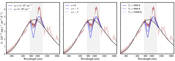
Figure A.2: VLT/X-shooter spectrum of AT2017gfo 4.4 days post merger with overlaid blackbody continuum ($T_{\rm BB}=3200$ K from best-fit blackbody temperature compilation in Sneppen et al. [66]) and P Cygni feature assuming $X_{\mathrm{He}}=0.01$ – but assuming a range of electron-densities ($n_{e}$, left panel), density power-law slopes ($\alpha$, center panel) and electron temperatures ($T_{e}$, right panel). For each panel, we assume the parameters from the other panel indicated with fully drawn lines (i.e. $n_{e}=1.5\times 10^{7}$ cm^-3, $\alpha=0$, $T_{e}=2800$ K). For the central panel, the reference electron density $n_{e}=1.5\times 10^{7}$ cm^-3 is at $0.19c$.

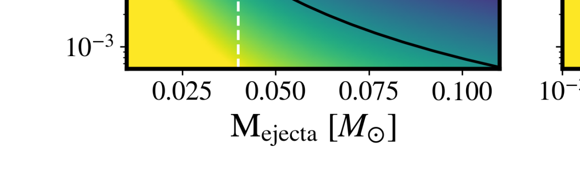
Figure A.3: Optical depth of He i $\lambda 1083.3$ nm line at photosphere given various ejecta properties, ie. helium mass fractions, $X_{\mathrm{He}}$, total ejecta-mass, $M_{\mathrm{ejecta}}$, radioactive heating deposited per unit time per ion, $\dot{q}$ (expressed at the value at 1 day post merger with the temporal decay following $t^{-1.3}$) and typical ionisation degree of the r-process elements, $Z_{\mathrm{ion}}$. We assume for these plots the powerlaw slope $\alpha=-5$ (from 0.1-0.5c) and that the typical nucleon weight has $A\sim 100$. The black contour-line indicates $\tau_{1083\,\mathrm{nm}}=1$, while the dotted white lines indicate the fiducial value of each parameter used for computations in the other panels. Lower ejecta masses, higher deposition-rates or lower ionisation degree increase the helium mass upper bound. The latter two parameters should not be considered independently as high deposition rates will also increase the typical ionisation degree of the r-process elements.

A.3 Estimating the electron density

In Fig. A.1, we show the electron-density as a function of velocity (at 1.5 and 4.4 days post-merger) given a simplified parametric ejecta distribution. Specifically, we assume a relatively low ionisation ejecta (i.e. $Z_{\mathrm{ion}}=2.5$, as characteristically expected from NLTE ionisation modeling, [70]) in which the average nucleon number is $A\sim 100$. We will assume that the ejecta have a density that follows a power-law distribution with radius, $\rho\,=\,\rho_{0}\,v^{\alpha}\,t^{-3}$ (ie. as in the main text), such that when integrated over volume (from 0.1c to 0.5c) it has a total ejecta mass similar to AT2017gfo (e.g. $\sim 0.04M_{\odot}$, [15, 80, 81]).The electron density is then related to the matter density as $n_{e}=Z_{\text{ion}}\rho/(Am_{u})$, with $m_{u}$ the atomic mass unit.

Figure A.1 highlights the two strongest functional dependencies in the electron-density. Firstly, the homologous expansion rapidly decreases the density in any layer ($\rho\propto t^{-3}$), which implies at late enough times the ejecta will reach low electron-densities and become inefficient at recombination. Secondly, for steep density gradients with velocity suggest a relatively consistent electron-densities in the receding line-forming region (these velocity regions inferred from the wavelength-range of the P Cygni are indicated with the black and green ranges in Fig. A.1). For instance, $n_{e}(0.3c,1.5\,d)\sim(2-6)\times\,n_{e}(0.19c,4.4\,d)$ for $\alpha$ between $-3$ and $-5$. This relatively slow temporal decline in the line-forming-region’s $n_{e}$ may be an important component behind the observed spectral features of AT2017gfo being remarkable consistent over such a large range of times and velocities [66]. Higher order effects like compositional variations shifting the characteristic nuclei number or deposition rate can affect the typical ionisation state, but these are of comparatively less importance. The variations in nucleon-number, $A$, and the typical ionisation-state, $Z_{\mathrm{ion}}$, is at most a factor of a few, while the heating rate per nucleon is rather consistent over a broad range of compositions for the time-scales of interest.

The rapid recombination from 1.43-1.47 days that appears to be needed to explain the observed Sr iii to Sr ii transition constrains the line-forming-region at this time and at these velocities ($v>0.3c$) to have an electron-density, $n_{e}\gtrsim 10^{8}\,$cm^-3 [66]. Assuming homologous expansion, these velocity-layers will be diluted $\sim 25$ fold by 4.4 days post-merger. However, the expectation from numerical hydro-simulations (see Sect. III) and lightcurve modeling of AT2017gfo, e.g. [80], is that the bulk of matter is ejected at lower velocities, so as the line-forming region recedes deeper into the ejecta the mass-density (and by extension $n_{e}$) should also increase. Whether $\rho\propto v^{-2}$ (i.e. equal mass at all radii) or a steeper radial decline, $\rho\propto v^{-5}$ [such as favored from lightcurve modeling, see 81], the resulting density at fixed time would be a factor of 2.5-10 (4-32) times greater at a velocity of 0.19c (0.15c) than 0.3c - implying $n_{e}\gtrsim 0.6-4\times 10^{7}\,{\rm cm}^{-3}$ ($n_{e}\gtrsim 1-13\times 10^{7}\,{\rm cm}^{-3}$) at $t=4.4$ days (if $n_{e}\gtrsim 10^{8}\,$cm^-3 at $0.3c$ and $t=1.5$ days). Given the output of any specific hydro-numerical simulation (or indeed any parametrized density structure) given an assumed typical ionisation state in the ejecta, one can estimate the electron density. For instance, the helium enriched models used for comparison with the hydro-simulations in Fig. 4, has a electron density ranging from $1.0\times 10^{7}$ cm^-3 to $7.8\times 10^{7}$ cm^-3 at 4.4 days across grid cells in the polar ejecta with velocities in the interval $0.19-0.3c$. These simulation based values are in close agreement with our simple estimates above.

A.4 P Cygni profiles sensitivity to assumed physical conditions

Ultimately, the electron density constraints presented in the paper are motivated by the observational constraints (e.g. recombination-timescales of features and existence of specific ionisation-states like Sr ii) and the typical ejecta-mass estimates for AT2017gfo. In Fig. A.2 (left panel), we show the strength of the P Cygni for various values of the photospheric electron-density, $n_{e}$. For sufficiently low electron density the strength of the feature diminishes. In Fig. A.2 central panel, we show the strength of the P Cygni for various power-law slopes, $\alpha$, characterizing the density decline in velocity space. Particularly, the blue wing of the absorption feature becomes weaker for more rapid declines - with a more negative $\alpha$ corresponding to a more rapid decline in the optical depth $\tau$ with velocity (ie. less scattering from higher velocity layers). However, the feature is not strongly sensitive to the assumption of the exact density distribution for a large range in $\alpha$ (including a steep decline, $\alpha=-5$, or an equal density at all radii $\alpha=0$) as long as the electron-density near the photosphere is not $\ll 6\times 10^{6}\,{\rm cm^{-3}}$. In Fig. A.2 (right panel), we show the strength of the P Cygni for various assumptions of the electron temperature used in the recombination-rate coefficient, $T_{e}$. Notably, the feature is weakest in the limit of low electron densities and high electron temperatures, as this produces the weakest recombination rates. We note the 2800 K assumed in the fiducial model is observationally motivated by the empirical goodness-of-fit for a simple blackbody model [208] and the 5-10 % consistency between electron and radiation temperature seen near ionisation transitions [65, 66], but nearly the same results are obtained across a broad temperature range.

In Fig. A.3, we highlight the robustness of our $X_{\text{He}}$ constraint on physical properties of the ejecta in another way. Here, we show the optical depth at the photosphere of the He i $\lambda 1083.3$ nm line given various helium mass fractions, total ejecta-mass, radioactive heating per unit time per ion and typical ionisation degree of the r-process elements. We assume for these plots the power-law slope $\alpha=-5$ (from 0.1-0.5c) and that the average nucleon-number is $A\sim 100$. A low ionisation state and lower total ejecta mass implies a smaller electron density, which in turn allows more helium to be hidden in the ejecta. Conversely, a lower deposition rate decreases the ionisation rate and thus suggest stronger bounds. Across a broad range of physical parameters we robustly obtain $\tau_{1083\,\mathrm{nm}}>1$ if $X_{\mathrm{He}}\gtrsim 0.05$.

Appendix B Hydrodynamic models used in Sect. III

Most of the merger models used in Sect. III to discuss the dependence of the helium mass fraction $X_{\mathrm{He}}$ on the HMNS-remnant lifetime $\tau_{\mathrm{BH}}$ are taken directly from Ref. [121], to which we refer for a detailed description of the model setup. The models are built from three-dimensional merger simulations (until 10 ms after merger), performed with a general relativistic SPH code [149] using a leakage-plus-absorption neutrino treatment [131] and assuming the conformal flatness condition, and two-dimensional (axisymmetric) simulations covering the post-merger (i.e. $>10\,$ms) evolution, conducted with a special-relativistic finite-volume code [209] adopting spectral M1 neutrino transport [132] and a gravitational potential that approximately reproduces general relativistic gravity [210].

With respect to Ref. [121] only the short-lived ($\tau_{\mathrm{BH}}=10\,$ms) models as well as the model without viscosity are new models. Each of the models listed in the legend of Fig. 5 is characterized through the model name as follows: Short-lived (“short”) models have a total mass of both NS progenitors of $M_{1}+M_{2}=2.8\,M_{\odot}$, while all others have $2.75\,M_{\odot}$; “sym” (“asy”) models have a mass ratio of $q=M_{1}/M_{2}=1$ ($q=0.75$); and the parameters used to describe the turbulent viscosity are indicated by the values after “n” and “a” (broadly speaking, the impact of viscosity is smaller for models with higher “n”- and lower “a”-values; cf. [121]). The suffix “novis” denotes the model with vanishing viscosity. In contrast to the long-lived models from Ref. [121], in which the time of BH formation is self-consistently obtained by the point when the HMNS becomes gravitationally unstable, in the “short” models we trigger an early collapse by hand by removing at $t=\tau_{\mathrm{BH}}=10\,$ms a small amount of material in the innermost part of the HMNS, which leads to an immediate collapse. Although this treatment is not fully hydrodynamically consistent, the impact on the resulting ejecta properties should be minor, because the total mass of the system that would actually collapse at $\tau_{\mathrm{BH}}=10\,$ms will only be a few percent higher than the $2.8\,M_{\odot}$ used for our current short-lived models.

In Fig. A.4 we provide mass-distribution histograms for a short- and a long-lived model, illustrating that the long-lived case is characterized by a distinct neutrino wind component at $Y_{e}\gtrsim 0.45$.

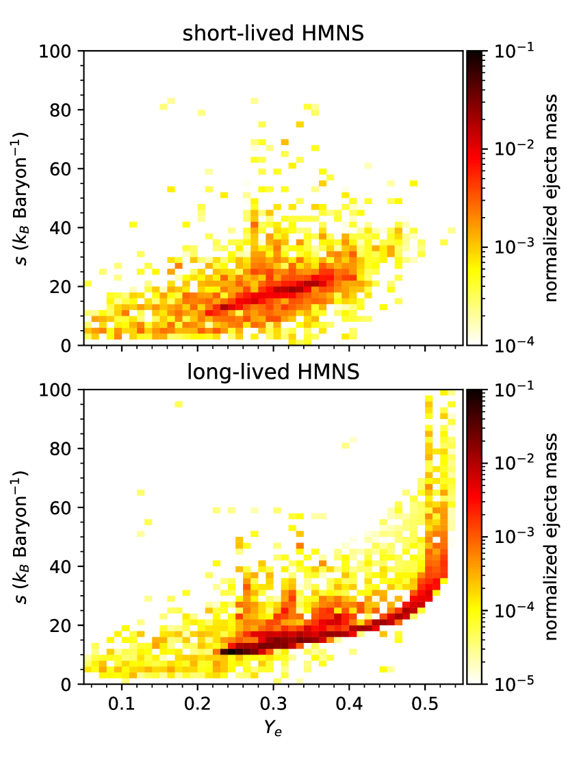
Figure A.4: Mass-distribution histograms in the space of electron fraction and entropy per baryon (both measured when the temperature drops below 5 GK) for ejecta material resulting in two numerical simulations in which the HMNS remnant is short-lived (model “sym-n1-a6-short” with $\tau_{\mathrm{BH}}=10$ ms; left panel) and long-lived (model “sym-n1-a6” with $\tau_{\mathrm{BH}}=122$ ms; right panel). The neutrino wind in the long-lived model produces a substantial amount of ejecta with $Y_{e}\gtrsim 0.45$.

The abundances of elements synthesized in the ejected material in the above hydrodynamical models are obtained in a post-processing step using the same methods as in Refs. [121] (called network B therein) and [211, 212]. To this end, a nuclear network calculation is run for about $\sim$5000–10000 tracer particles (per model) sampling the ejecta. For each trajectory, the full network is started at 8 GK to account for quasi-statistical equilibrium [93, 94]. The network assumes neutron-capture and photodissociation rates based on the HFB21 mass model [162] as described in [213], as well as the $\beta$-decay rates from [214].

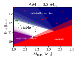
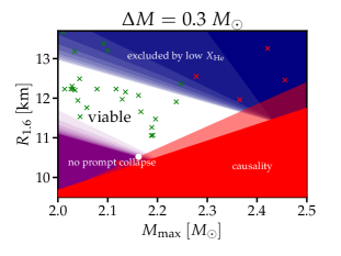
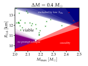
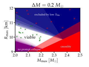
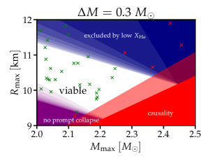
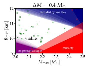
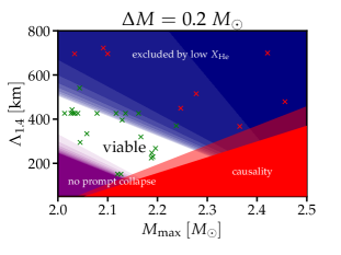
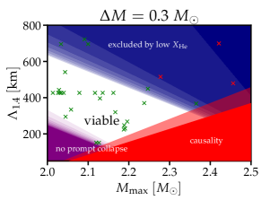
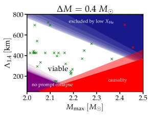
Figure A.5: Constraints on stellar parameters similar to Figs. 7 and 8 adopting $\Delta M=0.2\,$M_⊙ (left panels), $\Delta M=0.3\,$M_⊙ (middle panels) and $\Delta M=0.4\,$M_⊙ (right panels). Color shading of the blue and purple area indicates confidence levels of exclusion (in 10% steps) from considering the posterior distribution of the binary mass ratio of GW170817. Note the initial steep increase with the 50% level very close to the 10% level for the upper limit and the steep decrease between the 90% level and the 50% level for the lower limit. Green and red data points are stellar parameters from a large set of microphysical EoS models considered in [39]. Red crosses refer to EoS models which are excluded by our constraints. Dots in the upper row show which constraints are visualized in Figs. 9 and A.6 (see main text).

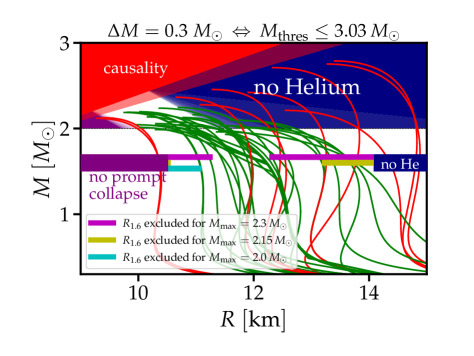
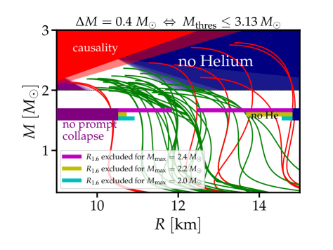
Figure A.6: Same as Fig. 9 but for $\Delta M=0.3\,$M_⊙ (left) and $\Delta M=0.4\,$M_⊙ (right). The adopted absolute $R_{1.6}$ constraints are displayed in Fig. A.5 by white dots (see main text for explanations). Note the different choices for $M_{\mathrm{max}}$ compared to Fig. 9 for which $R_{1.6}$ limits are displayed by the horizontal bars at $\approx 1.6~{}M_{\odot}$.

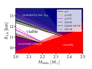
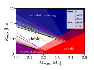
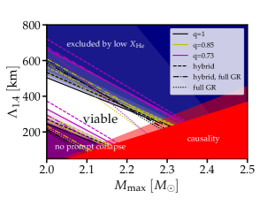
Figure A.7: Same as Figs. 7 and 8 but including alternative fit formulae for $M_{\mathrm{thres}}$ (assuming $\Delta M=0.2\,$M_⊙). Colors refer to fixed binary mass ratios of $q=1$ (black), $q=0.85$ (yellow) and $q=0.73$ (magenta). Solid lines adopt the same fit formula as in the main text (set ‘b’ in Tab. VI of [39]). For the dashed curves a fit formula is employ, which is based on data including nine EoS models with strong first-order phase transitions (set ‘b+h’ in Tab. VI of [39]). Dashed-dotted lines are obtained from the fit formula of [138] using the set ‘K+b+e+h’ (Tab. VIII). Note that most of the underlying data for this fit stems from [39]. Dotted curve results from a fit of [138] (set ‘K+P’, Tab. X).

Appendix C Sensitivity of EoS constraints

We provide additional plots exemplifying the sensitivity of our EoS constraints. In Fig. A.5 we show the limits on $R_{1.6}$, $R_{\mathrm{max}}$ and $\Lambda_{1.4}$ adopting different values for $\Delta M$, i.e. the proximity of the measured total binary mass of GW170817 to the threshold mass for prompt black hole formation. As expected from Eq. (5), the upper limits become less constraining if $\Delta M$ increases although even for the very conservative case of $\Delta M=0.4\,$M_⊙ the absence of significant amounts of helium in the ejecta still excludes some current microphysical EoS models which are compatible with pulsar observations [183, 184, 185] and the tidal deformability inference from GW170817 [9]. For better illustration in Fig. A.5 we overplot stellar parameters from a set of microphysical EoSs (same EoS sample as in [39], i.e. the identical set that was employed to construct fit formulae for $M_{\mathrm{thres}}$ in [39]). These panels also demonstrate the potential of our limits, which place a combined constraint on $R/\Lambda$ and $M_{\mathrm{max}}$. For instance, some models with $R_{1.6}\sim 12$ km are excluded because their $M_{\mathrm{max}}$ is too large.

The lower limits on $R/\Lambda$ are independent of $\Delta M$ because they are solely based on the argument that GW170817 did not undergo a prompt collapse. Imposing additionally that the EoS cannot become arbitrarily stiff, which is ultimately limited by causality, rules out stellar parameters in the lower right corner of the panels. We distinguish between a more conservative “causality limit” adopting $v_{s}=c$ above a certain density and a more empirical relation which simply reproduces the stellar parameter found in a large set of microphysical candidate EoSs (light shading). See [36, 39] for more detailed explanations.

In brief, we obtain the “causality” limit by the following consideration. For a given $R_{1.6}$, the maximum mass cannot become too large with the maximum $M_{\mathrm{max}}^{\mathrm{up}}(R_{1.6})$ given by a fiducial stellar configuration that has maximal stiffness, i.e. $v_{\mathrm{s}}=c$, beyond the central density of the 1.6 M_⊙ NS. For a large set of microphysical EoSs (the sample used in [39]), we adopt the EoS up to the central density of the 1.6 M_⊙ NS and extend the EoS to higher densities imposing $v_{\mathrm{s}}=c$. From this modified EoS we obtain the Tolman-Oppenheimer-Volkoff (TOV) solution with the highest possible $M_{\mathrm{max}}^{\mathrm{up}}$. Considering the pairs $\{R_{1.6},M_{\mathrm{max}}^{\mathrm{up}}\}$ for the full set of modified EoSs, we determine a line with coefficients $w_{1}$ and $w_{2}$ such that $M_{\mathrm{max}}^{\mathrm{up}}(R)<w_{1}R+w_{2}$. Being less conservative, we obtain a second set of $w_{1}$ and $w_{2}$ as an “empirical” limit by considering the original pairs $\{R_{1.6},M_{\mathrm{max}}\}$ with the actual $M_{\mathrm{max}}$ from the unmodified, microphysical EoS. None of the actual models (green crosses) lies beyond the light red area in Fig. A.5. The constraints are quantified as $M_{\mathrm{max}}(R)\leq w_{1}R+w_{2}$ (and equivalently for $\Lambda$) with $w_{1}$ and $w_{2}$ provided in Tab. 2; for $R_{\mathrm{max}}$ we adopt the result from [187, 4]. The exact limits obviously depend on the chosen set of EoS models and for consistency we here repeat the procedure for the EoS sample from [39]. Determining the lines to embrace all models for the conservative and the empirical limit is obviously ambiguous. Finally, for a given EoS model with a given $R_{1.6}$, the computation of $M_{\mathrm{max}}^{\mathrm{up}}(R_{1.6})$ as described may not exactly yield the highest possible $M_{\mathrm{max}}$ because a different EoS at lower densities with the same $R_{1.6}$ may yield a slightly larger limit. However, all these effects are relatively small in practice and the displayed areas thus provide very reasonable limits.

The intersections of these limits with the bound from the no-prompt-collapse constraint provide absolute lower limits on $R/\Lambda$ (see Fig. A.5). We list these limits in Tab. 2 together with the absolute upper limits, i.e. the constraints for $M_{\mathrm{max}}=2.0\,$M_⊙ for different values of $\Delta M$. All limits adopt the 90% confidence level resulting form the posterior distribution of the binary mass ratio of GW170817. The table also provides the absolute upper limits on the maximum mass $M_{\mathrm{max}}$, which is given by the intersection of the upper limit $R/\Lambda$ limit with the causality (or empirical) constraint (see Fig. A.5). For a given $\Delta M$, these limits slightly depend on whether one determines the intersection with the upper bound on $R_{1.6}$, $R_{\mathrm{max}}$ or $\Lambda_{1.4}$ (with the corresponding $w_{1}$ and $w_{2}$). However, comparing the constraints on $M_{\mathrm{max}}$ for the respective causal or empirical limit, one finds a very good agreement between these numbers. For instance, we find $M_{\mathrm{max}}\lesssim 2.31$, $M_{\mathrm{max}}\lesssim 2.38$ and $M_{\mathrm{max}}\lesssim 2.45$ for $\Delta M=0.2\,$M_⊙, $\Delta M=0.3\,$M_⊙ and $\Delta M=0.4\,$M_⊙, respectively, adopting the empirical relations.

For the cases $\Delta M=0.3\,$M_⊙ and $\Delta M=0.4\,$M_⊙ we visualize the resulting constraints in comparison to mass-radius relations from existing microphysical EoSs in Fig. A.6. These plots are equivalent to Fig. 9 with the same color scheme as in the main text, to which we refer for further explanations.

Figure A.7 exemplifies the impact of other fit formulae for $M_{\mathrm{thres}}$ on the different constraints for $R_{1.6}$, $R_{\mathrm{max}}$ and $\Lambda_{1.4}$ adopting $\Delta M=0.2\,$M_⊙. See Tab. 1 for fits and coefficients. Different colors of the lines again refer to fixed binary mass ratios and the solid curves display the limits resulting from the fit formulae used in the main text and Figs. A.5 and A.6. For the dashed lines we employ fit formulae based on a dataset which includes EoS models undergoing a strong phase transition to deconfined quark matter (set ‘b+h’ in Tab. VI of [39]). The resulting constraints become slightly weaker in particular for relatively small $M_{\mathrm{max}}\approx 2.0\,$M_⊙. We do not adopt these fit formulae as our standard choice because the additional hybrid models considered in these fits are on the rather extreme side with regard to the stiffness of the quark matter EoS (see [215]) and thus possibly represent an unlikely range of models. The dashed-dotted lines in Fig. A.7 display the results from using the fit formulae (set ‘K+b+e+h’) from Ref. [138]. These fits are based on data, which include $M_{\mathrm{thres}}$ determinations from different simulation tools. Most models are taken from [39] but also fully relativistic models are computed. Note that the set include hybrid models as well. The dotted lines correspond to fits to a dataset which only comprises fully relativistic calculations (set ‘K=P’ from [138]) as opposed to the approximate solution of the Einstein equations within the conformal flatness approximation in [39]. We do not consider these fits as default choice because they are based on a significantly smaller number of EoS models and calculations for a wider range of binary mass ratios, which is not required for the range inferred from GW170817. Thus, the coverage of the range in $q$ and EoSs models applicable to our constraints is not as comprehensive as the on in [39]. Note that the comparisons in [138, 142] show a generally very good agreement between the calculations in full general relativity and the ones within the conformal flatness approximation [142]. At any rate our plots (Fig. A.7) show that the main uncertainties originate form the unknown $M_{\mathrm{max}}$ and binary mass ratio $q$.

$X$	$c_{1}$	$c_{2}$	$c_{3}$	$c_{4}$	$c_{5}$	$c_{6}$	$c_{7}$	dev.	Ref.
$M_{\mathrm{thres}}(q,M_{\mathrm{max}},X)=c_{1}M_{\mathrm{max}}+c_{2}X+c_{3}+c_{4}\delta q^{3}M_{\mathrm{max}}+c_{5}\delta q^{3}X$
$R_{1.6}$	0.578	$1.610\times 10^{-1}$	-0.218	8.987	-1.767	-	-	0.017	[39]
$R_{\mathrm{max}}$	0.491	$1.847\times 10^{-1}$	-0.051	9.382	-2.088	-	-	0.021	[39]
$\Lambda_{1.4}$	0.698	$7.772\times 10^{-4}$	1.137	0.900	$-9.050\times 10^{-3}$	-	-	0.029	[39]
$R_{1.6}$ hybrid	0.663	$1.535\times 10^{-1}$	-0.329	9.058	-1.784	-	-	0.035	[39]
$R_{\mathrm{max}}$ hybrid	0.613	$1.665\times 10^{-1}$	-0.135	8.209	-1.859	-	-	0.032	[39]
$\Lambda_{1.4}$ hybrid	0.750	$7.670\times 10^{-4}$	1.016	0.878	$-9.763\times 10^{-3}$	-	-	0.040	[39]
$R_{1.6}$ hybrid, full GR	0.675	$1.500\times 10^{-1}$	-0.315	5.313	-1.031	-	-	0.0365	[138]
$\Lambda_{1.4}$ hybrid, full GR	0.67	$5.338\times 10^{-4}$	1.271	-0.042	$-3.347\times 10^{-4}$	-	-	0.0456	[138]
$M_{\mathrm{thres}}(q,M_{\mathrm{max}},X)=c_{1}M_{\mathrm{max}}+c_{2}X+c_{3}+c_{4}\delta qM_{\mathrm{max}}+c_{5}\delta qX+c_{6}\delta q^{3}M_{\mathrm{max}}+c_{7}\delta q^{3}X$
$R_{1.6}$ full GR	0.462	0.14	0.251	0.76	-0.12	0.00817	-0.188	0.0287	[138]
$R_{\mathrm{max}}$ full GR	0.428	0.134	0.602	0.886	-0.16	-0.539	-0.112	0.0341	[138]
$\Lambda_{1.4}$ full GR	0.686	$5.049\times 10^{-4}$	1.249	0.162	$-3.921\times 10^{-4}$	-0.808	$-1.406\times 10^{-3}$	0.0303	[138]

Table 1: Different fits describing the EoS dependence of the threshold binary mass $M_{\mathrm{thres}}$ for prompt BH formation including an explicit dependence on the binary mass ratio $q$ through $\delta q=1-q$ (see main text). First column specifies the stellar parameter $X$, which may either be $R_{1.6}$, $R_{\mathrm{max}}$ or $\Lambda_{1.4}$ and the underlying set of data (see caption of Fig. A.7). Fit parameters $c_{i}$ are given in second to eighth columns. The units of the fit parameters $c_{i}$ are such that masses are in M_⊙, radii in km and tidal deformabilities dimensionless. Next column specifies the average deviation between fit and the underlying data. Last column provides the reference from which the fit is taken and where further details can be found.

Table 2: Absolute lower and upper limits on different stellar parameters $X$ independent of $M_{\mathrm{max}}$ for different $\Delta M$ (see main text). Radii are given in km. $w_{1}$ and $w_{2}$ describe an upper limit on the maximum mass via $M_{\mathrm{max}}\leq w_{1}X+w_{2}$. ‘causal’ and ‘empirical’ in the first column indicate how $w_{1}$ and $w_{2}$ were obtained, where ‘causal’ implies a more conservative approach and limit on $X$ assuming maximum stiffness of the EoS at higher densities and ‘empirical’ only embraces a large but incomplete set of currently available microphysical models. Every combination $\Delta M$, $w_{1}$ and $w_{2}$ determines an absolute upper limit on $M_{\mathrm{max}}$ (in solar masses) listed after the rows with the corresponding limits on $R_{1.6}$, $R_{\mathrm{max}}$ and $\Lambda_{1.4}$ for the same set of $\Delta M$, $w_{1}$ and $w_{2}$. All limits are determined adopting the 90% confidence level resulting from the distribution of the binary mass ratio of GW170817.

Parameter (limit)	$\Delta M/M_{\odot}$	lower limit	upper limit	$w_{1}$	$w_{2}$
$R_{1.6}$ (causal)	0.2	10.44	13.29	0.241	-0.336
$R_{1.6}$ (empirical)	0.2	10.52	13.29	0.179	0.282
$M_{\mathrm{max}}$ (causal)	0.2	-	2.353	0.241	-0.336
$M_{\mathrm{max}}$ (empirical)	0.2	-	2.316	0.179	0.282
$R_{\mathrm{max}}$ (causal)	0.2	9.17	11.63	0.240	0.0
$R_{\mathrm{max}}$ (empirical)	0.2	9.31	11.63	0.197	0.321
$M_{\mathrm{max}}$ (causal)	0.2	-	2.369	0.240	0.0
$M_{\mathrm{max}}$ (empirical)	0.2	-	2.313	0.197	0.321
$\Lambda_{1.4}$ (causal)	0.2	117.0	668.7	0.0014	1.982
$\Lambda_{1.4}$ (empirical)	0.2	131.4	668.7	0.0011	1.980
$M_{\mathrm{max}}$ (causal)	0.2	-	2.341	0.0014	1.982
$M_{\mathrm{max}}$ (empirical)	0.2	-	2.312	0.0011	1.980
$R_{1.6}$ (causal)	0.3	10.44	14.08	0.241	-0.336
$R_{1.6}$ (empirical)	0.3	10.52	14.08	0.179	0.282
$R_{1.6}$ (causal)	0.3	-	2.431	0.241	-0.336
$R_{1.6}$ (empirical)	0.3	-	2.384	0.179	0.282
$R_{\mathrm{max}}$ (causal)	0.3	9.17	12.33	0.240	0.0
$R_{\mathrm{max}}$ (empirical)	0.3	9.31	12.33	0.197	0.321
$R_{\mathrm{max}}$ (causal)	0.3	-	2.447	0.240	0.0
$R_{\mathrm{max}}$ (empirical)	0.3	-	2.384	0.197	0.321
$\Lambda_{1.4}$ (causal)	0.3	117.0	837.2	0.0014	1.982
$\Lambda_{1.4}$ (empirical)	0.3	131.4	837.2	0.0011	1.980
$\Lambda_{1.4}$ (causal)	0.3	-	2.429	0.0014	1.982
$\Lambda_{1.4}$ (empirical)	0.3	-	2.393	0.0011	1.980
$R_{1.6}$ (causal)	0.4	10.44	14.82	0.241	-0.336
$R_{1.6}$ (empirical)	0.4	10.52	14.82	0.179	0.282
$R_{1.6}$ (causal)	0.4	-	2.509	0.241	-0.336
$R_{1.6}$ (empirical)	0.4	-	2.453	0.179	0.282
$R_{\mathrm{max}}$ (causal)	0.4	9.17	13.03	0.240	0.0
$R_{\mathrm{max}}$ (empirical)	0.4	9.31	13.03	0.197	0.321
$R_{\mathrm{max}}$ (causal)	0.4	-	2.526	0.240	0.0
$R_{\mathrm{max}}$ (empirical)	0.4	-	2.455	0.197	0.321
$\Lambda_{1.4}$ (causal)	0.4	117.0	1005.5	0.0014	1.982
$\Lambda_{1.4}$ (empirical)	0.4	131.4	1005.5	0.0011	1.980
$\Lambda_{1.4}$ (causal)	0.4	-	2.517	0.0014	1.982
$\Lambda_{1.4}$ (empirical)	0.4	-	2.473	0.0011	1.980

References

- Tolman [1939] R. C. Tolman, Static solutions of Einstein’s field equations for spheres of fluid, Phys. Rev. 55, 364 (1939).
- Oppenheimer and Volkoff [1939] J. R. Oppenheimer and G. M. Volkoff, On massive neutron cores, Phys. Rev. 55, 374 (1939).
- Hinderer et al. [2010] T. Hinderer, B. D. Lackey, R. N. Lang, and J. S. Read, Tidal deformability of neutron stars with realistic equations of state and their gravitational wave signatures in binary inspiral, Phys. Rev. D 81, 123016 (2010), arXiv:0911.3535 [astro-ph.HE] .
- Lattimer and Prakash [2016] J. M. Lattimer and M. Prakash, The equation of state of hot, dense matter and neutron stars, Phys. Rep. 621, 127 (2016), arXiv:1512.07820 [astro-ph.SR] .
- Baym et al. [2018] G. Baym, T. Hatsuda, T. Kojo, P. D. Powell, Y. Song, and T. Takatsuka, From hadrons to quarks in neutron stars: a review, Rept. Prog. Phys. 81, 056902 (2018), arXiv:1707.04966 [astro-ph.HE] .
- Oertel et al. [2017] M. Oertel, M. Hempel, T. Klähn, and S. Typel, Equations of state for supernovae and compact stars, Rev. Mod. Phys. 89, 015007 (2017), arXiv:1610.03361 [astro-ph.HE] .
- Raduta [2022] A. R. Raduta, Equations of state for hot neutron stars-II. The role of exotic particle degrees of freedom, Eur. Phys. J. A 58, 115 (2022), arXiv:2205.03177 [nucl-th] .
- Abbott et al. [2017] B. P. Abbott et al. (LIGO Scientific Collaboration and Virgo Collaboration), Gw170817: Observation of gravitational waves from a binary neutron star inspiral, Phys. Rev. Lett. 119, 161101 (2017).
- Abbott et al. [2019] B. P. Abbott et al. (LIGO Scientific Collaboration and Virgo Collaboration), Properties of the binary neutron star merger gw170817, Phys. Rev. X 9, 011001 (2019).
- Abbott et al. [2018] B. P. Abbott et al. (The LIGO Scientific Collaboration and the Virgo Collaboration), Gw170817: Measurements of neutron star radii and equation of state, Phys. Rev. Lett. 121, 161101 (2018).
- De et al. [2018] S. De, D. Finstad, J. M. Lattimer, D. A. Brown, E. Berger, and C. M. Biwer, Tidal Deformabilities and Radii of Neutron Stars from the Observation of GW170817, Phys. Rev. Lett. 121, 091102 (2018), arXiv:1804.08583 [astro-ph.HE] .
- Coulter et al. [2017] D. A. Coulter, R. J. Foley, C. D. Kilpatrick, M. R. Drout, A. L. Piro, B. J. Shappee, M. R. Siebert, J. D. Simon, N. Ulloa, D. Kasen, B. F. Madore, A. Murguia-Berthier, Y. C. Pan, J. X. Prochaska, E. Ramirez-Ruiz, A. Rest, and C. Rojas-Bravo, Swope Supernova Survey 2017a (SSS17a), the optical counterpart to a gravitational wave source, Science 358, 1556 (2017), arXiv:1710.05452 [astro-ph.HE] .
- Andreoni et al. [2017] I. Andreoni et al., Follow Up of GW170817 and Its Electromagnetic Counterpart by Australian-Led Observing Programmes, PASA 34, e069 (2017), arXiv:1710.05846 [astro-ph.HE] .
- Buckley et al. [2018] D. A. H. Buckley, I. Andreoni, S. Barway, J. Cooke, S. M. Crawford, E. Gorbovskoy, M. Gromadzki, V. Lipunov, J. Mao, S. B. Potter, M. L. Pretorius, T. A. Pritchard, E. Romero-Colmenero, M. M. Shara, P. Väisänen, and T. B. Williams, A comparison between SALT/SAAO observations and kilonova models for AT 2017gfo: the first electromagnetic counterpart of a gravitational wave transient - GW170817, Mon. Not. R. Astron. Soc. 474, L71 (2018), arXiv:1710.05855 [astro-ph.HE] .
- Cowperthwaite et al. [2017] P. S. Cowperthwaite et al., The Electromagnetic Counterpart of the Binary Neutron Star Merger LIGO/Virgo GW170817. II. UV, Optical, and Near-infrared Light Curves and Comparison to Kilonova Models, Astrophys. J. Lett. 848, L17 (2017), arXiv:1710.05840 [astro-ph.HE] .
- Drout et al. [2017] M. R. Drout et al., Light curves of the neutron star merger GW170817/SSS17a: Implications for r-process nucleosynthesis, Science 358, 1570 (2017), arXiv:1710.05443 [astro-ph.HE] .
- Kasen et al. [2017] D. Kasen, B. Metzger, J. Barnes, E. Quataert, and E. Ramirez-Ruiz, Origin of the heavy elements in binary neutron-star mergers from a gravitational-wave event, Nature (London) 551, 80 (2017), arXiv:1710.05463 [astro-ph.HE] .
- Kasliwal et al. [2017] M. M. Kasliwal et al., Illuminating gravitational waves: A concordant picture of photons from a neutron star merger, Science 358, 1559 (2017), arXiv:1710.05436 [astro-ph.HE] .
- Kilpatrick et al. [2017] C. D. Kilpatrick, R. J. Foley, D. Kasen, A. Murguia-Berthier, E. Ramirez-Ruiz, D. A. Coulter, M. R. Drout, A. L. Piro, B. J. Shappee, K. Boutsia, C. Contreras, F. Di Mille, B. F. Madore, N. Morrell, Y. C. Pan, J. X. Prochaska, A. Rest, C. Rojas-Bravo, M. R. Siebert, J. D. Simon, and N. Ulloa, Electromagnetic evidence that SSS17a is the result of a binary neutron star merger, Science 358, 1583 (2017), arXiv:1710.05434 [astro-ph.HE] .
- Nicholl et al. [2017] M. Nicholl, E. Berger, D. Kasen, B. D. Metzger, J. Elias, C. Briceño, K. D. Alexander, P. K. Blanchard, R. Chornock, P. S. Cowperthwaite, T. Eftekhari, W. Fong, R. Margutti, V. A. Villar, P. K. G. Williams, W. Brown, J. Annis, A. Bahramian, D. Brout, D. A. Brown, H. Y. Chen, J. C. Clemens, E. Dennihy, B. Dunlap, D. E. Holz, E. Marchesini, F. Massaro, N. Moskowitz, I. Pelisoli, A. Rest, F. Ricci, M. Sako, M. Soares-Santos, and J. Strader, The Electromagnetic Counterpart of the Binary Neutron Star Merger LIGO/Virgo GW170817. III. Optical and UV Spectra of a Blue Kilonova from Fast Polar Ejecta, Astrophys. J. Lett. 848, L18 (2017), arXiv:1710.05456 [astro-ph.HE] .
- Pian et al. [2017] E. Pian et al., Spectroscopic identification of r-process nucleosynthesis in a double neutron-star merger, Nature (London) 551, 67 (2017), arXiv:1710.05858 [astro-ph.HE] .
- Shappee et al. [2017] B. J. Shappee et al., Early spectra of the gravitational wave source GW170817: Evolution of a neutron star merger, Science 358, 1574 (2017), arXiv:1710.05432 [astro-ph.HE] .
- Smartt et al. [2017] S. J. Smartt et al., A kilonova as the electromagnetic counterpart to a gravitational-wave source, Nature (London) 551, 75 (2017), arXiv:1710.05841 [astro-ph.HE] .
- Soares-Santos et al. [2017] M. Soares-Santos et al. (Dark Energy Survey and Dark Energy Camera GW-EM Collaboration), The Electromagnetic Counterpart of the Binary Neutron Star Merger LIGO/Virgo GW170817. I. Discovery of the Optical Counterpart Using the Dark Energy Camera, Astrophys. J. Lett. 848, L16 (2017), arXiv:1710.05459 [astro-ph.HE] .
- Tanaka et al. [2017] M. Tanaka et al., Kilonova from post-merger ejecta as an optical and near-Infrared counterpart of GW170817, PASJ 69, 102 (2017).
- Tanvir et al. [2017] N. R. Tanvir et al., The Emergence of a Lanthanide-rich Kilonova Following the Merger of Two Neutron Stars, Astrophys. J. Lett. 848, L27 (2017), arXiv:1710.05455 [astro-ph.HE] .
- Horowitz et al. [2019] C. J. Horowitz et al., r-process nucleosynthesis: connecting rare-isotope beam facilities with the cosmos, J. Phys. G: Nucl. Part. Phys. 46, 083001 (2019).
- Arnould and Goriely [2020] M. Arnould and S. Goriely, Astronuclear Physics: A tale of the atomic nuclei in the skies, Progress in Particle and Nuclear Physics 112, 103766 (2020).
- Cowan et al. [2021] J. J. Cowan, C. Sneden, J. E. Lawler, A. Aprahamian, M. Wiescher, K. Langanke, G. Martínez-Pinedo, and F.-K. Thielemann, Origin of the heaviest elements: The rapid neutron-capture process, Reviews of Modern Physics 93, 015002 (2021), arXiv:1901.01410 [astro-ph.HE] .
- Li and Paczyński [1998] L.-X. Li and B. Paczyński, Transient Events from Neutron Star Mergers, Astrophys. J. Lett. 507, L59 (1998).
- Kulkarni [2005] S. R. Kulkarni, Modeling Supernova-like Explosions Associated with Gamma-ray Bursts with Short Durations, ArXiv Astrophysics e-prints , arXiv:astro (2005).
- Metzger et al. [2010] B. D. Metzger, G. Martínez-Pinedo, S. Darbha, E. Quataert, A. Arcones, D. Kasen, R. Thomas, P. Nugent, I. V. Panov, and N. T. Zinner, Electromagnetic counterparts of compact object mergers powered by the radioactive decay of r-process nuclei, Mon. Not. R. Astron. Soc. 406, 2650 (2010), arXiv:1001.5029 [astro-ph.HE] .
- Bauswein et al. [2017] A. Bauswein, O. Just, H.-T. Janka, and N. Stergioulas, Neutron-star Radius Constraints from GW170817 and Future Detections, Astrophys. J. Lett. 850, L34 (2017), arXiv:1710.06843 [astro-ph.HE] .
- Radice et al. [2018a] D. Radice, A. Perego, F. Zappa, and S. Bernuzzi, GW170817: Joint Constraint on the Neutron Star Equation of State from Multimessenger Observations, Astrophys. J. Lett. 852, L29 (2018a), arXiv:1711.03647 [astro-ph.HE] .
- Köppel et al. [2019] S. Köppel, L. Bovard, and L. Rezzolla, A General-relativistic Determination of the Threshold Mass to Prompt Collapse in Binary Neutron Star Mergers, Astrophys. J. Lett. 872, L16 (2019), arXiv:1901.09977 [gr-qc] .
- Bauswein [2019] A. Bauswein, Equation of state constraints from multi-messenger observations of neutron star mergers, Annals of Physics 411, 167958 (2019), arXiv:2103.16371 [astro-ph.HE] .
- Capano et al. [2020] C. D. Capano, I. Tews, S. M. Brown, B. Margalit, S. De, S. Kumar, D. A. Brown, B. Krishnan, and S. Reddy, Stringent constraints on neutron-star radii from multimessenger observations and nuclear theory, Nature Astronomy 4, 625 (2020), arXiv:1908.10352 [astro-ph.HE] .
- Kiuchi et al. [2019] K. Kiuchi, K. Kyutoku, M. Shibata, and K. Taniguchi, Revisiting the lower bound on tidal deformability derived by AT 2017gfo, Astrophys. J. Lett. 876, L31 (2019), arXiv:1903.01466 [astro-ph.HE] .
- Bauswein et al. [2021] A. Bauswein, S. Blacker, G. Lioutas, T. Soultanis, V. Vijayan, and N. Stergioulas, Systematics of prompt black-hole formation in neutron star mergers, Phys. Rev. D 103, 123004 (2021), arXiv:2010.04461 [astro-ph.HE] .
- Spitkovsky [2006] A. Spitkovsky, Time-dependent Force-free Pulsar Magnetospheres: Axisymmetric and Oblique Rotators, Astrophys. J. Lett. 648, L51 (2006).
- Margalit and Metzger [2017] B. Margalit and B. D. Metzger, Constraining the Maximum Mass of Neutron Stars from Multi-messenger Observations of GW170817, Astrophys. J. Lett. 850, L19 (2017), arXiv:1710.05938 [astro-ph.HE] .
- Shibata et al. [2017] M. Shibata, S. Fujibayashi, K. Hotokezaka, K. Kiuchi, K. Kyutoku, Y. Sekiguchi, and M. Tanaka, Modeling GW170817 based on numerical relativity and its implications, Phys. Rev. D 96, 123012 (2017), arXiv:1710.07579 [astro-ph.HE] .
- Shibata et al. [2019] M. Shibata, E. Zhou, K. Kiuchi, and S. Fujibayashi, Constraint on the maximum mass of neutron stars using GW170817 event, Phys. Rev. D 100, 023015 (2019), arXiv:1905.03656 [astro-ph.HE] .
- Margalit et al. [2022] B. Margalit, A. S. Jermyn, B. D. Metzger, L. F. Roberts, and E. Quataert, Angular-momentum Transport in Proto-neutron Stars and the Fate of Neutron Star Merger Remnants, Astrophys. J. 939, 51 (2022), arXiv:2206.10645 [astro-ph.HE] .
- Rezzolla et al. [2018] L. Rezzolla, E. R. Most, and L. R. Weih, Using Gravitational-wave Observations and Quasi-universal Relations to Constrain the Maximum Mass of Neutron Stars, Astrophys. J. Lett. 852, L25 (2018), arXiv:1711.00314 [astro-ph.HE] .
- Ruiz et al. [2018] M. Ruiz, S. L. Shapiro, and A. Tsokaros, GW170817, general relativistic magnetohydrodynamic simulations, and the neutron star maximum mass, Phys. Rev. D 97, 021501 (2018), arXiv:1711.00473 [astro-ph.HE] .
- Duncan and Thompson [1992] R. C. Duncan and C. Thompson, Formation of Very Strongly Magnetized Neutron Stars: Implications for Gamma-Ray Bursts, Astrophys. J. Lett. 392, L9 (1992).
- Metzger et al. [2008a] B. D. Metzger, E. Quataert, and T. A. Thompson, Short-duration gamma-ray bursts with extended emission from protomagnetar spin-down, Mon. Not. R. Astron. Soc. 385, 1455 (2008a), arXiv:0712.1233 [astro-ph] .
- Kiuchi et al. [2024] K. Kiuchi, A. Reboul-Salze, M. Shibata, and Y. Sekiguchi, A large-scale magnetic field produced by a solar-like dynamo in binary neutron star mergers, Nature Astronomy (2024).
- Coughlin et al. [2018] M. W. Coughlin, T. Dietrich, Z. Doctor, D. Kasen, S. Coughlin, A. Jerkstrand, G. Leloudas, O. McBrien, B. D. Metzger, R. O’Shaughnessy, and S. J. Smartt, Constraints on the neutron star equation of state from AT2017gfo using radiative transfer simulations, Mon. Not. R. Astron. Soc. 480, 3871 (2018), arXiv:1805.09371 [astro-ph.HE] .
- Radice and Dai [2019] D. Radice and L. Dai, Multimessenger parameter estimation of GW170817, European Physical Journal A 55, 50 (2019), arXiv:1810.12917 [astro-ph.HE] .
- Dietrich et al. [2020] T. Dietrich, M. W. Coughlin, P. T. H. Pang, M. Bulla, J. Heinzel, L. Issa, I. Tews, and S. Antier, Multimessenger constraints on the neutron-star equation of state and the Hubble constant, Science 370, 1450 (2020), arXiv:2002.11355 [astro-ph.HE] .
- Breschi et al. [2021] M. Breschi, A. Perego, S. Bernuzzi, W. Del Pozzo, V. Nedora, D. Radice, and D. Vescovi, AT2017gfo: Bayesian inference and model selection of multicomponent kilonovae and constraints on the neutron star equation of state, Mon. Not. R. Astron. Soc. 505, 1661 (2021), arXiv:2101.01201 [astro-ph.HE] .
- Raaijmakers et al. [2021] G. Raaijmakers, S. K. Greif, K. Hebeler, T. Hinderer, S. Nissanke, A. Schwenk, T. E. Riley, A. L. Watts, J. M. Lattimer, and W. C. G. Ho, Constraints on the Dense Matter Equation of State and Neutron Star Properties from NICER’s Mass-Radius Estimate of PSR J0740+6620 and Multimessenger Observations, Astrophys. J. Lett. 918, L29 (2021), arXiv:2105.06981 [astro-ph.HE] .
- Huth et al. [2022] S. Huth, P. T. H. Pang, I. Tews, T. Dietrich, A. Le Fèvre, A. Schwenk, W. Trautmann, K. Agarwal, M. Bulla, M. W. Coughlin, and C. Van Den Broeck, Constraining neutron-star matter with microscopic and macroscopic collisions, Nature (London) 606, 276 (2022), arXiv:2107.06229 [nucl-th] .
- Lund et al. [2024] K. A. Lund, R. Somasundaram, G. C. McLaughlin, J. M. Miller, M. R. Mumpower, and I. Tews, Kilonova Emissions from Neutron Star Merger Remnants: Implications for Nuclear Equation of State, arXiv e-prints , arXiv:2408.07686 (2024).
- Henkel et al. [2023] A. Henkel, F. Foucart, G. Raaijmakers, and S. Nissanke, Study of the agreement between binary neutron star ejecta models derived from numerical relativity simulations, Phys. Rev. D 107, 063028 (2023), arXiv:2207.07658 [astro-ph.HE] .
- Janka and Bauswein [2022] H. T. Janka and A. Bauswein, Dynamics and Equation of State Dependencies of Relevance for Nucleosynthesis in Supernovae and Neutron Star Mergers, arXiv e-prints , arXiv:2212.07498 (2022), arXiv:2212.07498 [astro-ph.HE] .
- Holmbeck et al. [2021] E. M. Holmbeck, A. Frebel, G. C. McLaughlin, R. Surman, R. Fernández, B. D. Metzger, M. R. Mumpower, and T. M. Sprouse, Reconstructing masses of merging neutron stars from stellar r-process abundance signatures, The Astrophysical Journal 909, 21 (2021).
- Levan et al. [2024] A. J. Levan et al., Heavy-element production in a compact object merger observed by JWST, Nature (London) 626, 737 (2024), arXiv:2307.02098 [astro-ph.HE] .
- Watson et al. [2019] D. Watson, C. J. Hansen, J. Selsing, A. Koch, D. B. Malesani, A. C. Andersen, J. P. U. Fynbo, A. Arcones, A. Bauswein, S. Covino, A. Grado, K. E. Heintz, L. Hunt, C. Kouveliotou, G. Leloudas, A. J. Levan, P. Mazzali, and E. Pian, Identification of strontium in the merger of two neutron stars, Nature (London) 574, 497 (2019), arXiv:1910.10510 [astro-ph.HE] .
- Domoto et al. [2021] N. Domoto, M. Tanaka, S. Wanajo, and K. Kawaguchi, Signatures of r-process Elements in Kilonova Spectra, Astrophys. J. 913, 26 (2021), arXiv:2103.15284 [astro-ph.HE] .
- Gillanders et al. [2022] J. H. Gillanders, S. J. Smartt, S. A. Sim, A. Bauswein, and S. Goriely, Modelling the spectra of the kilonova AT2017gfo - I. The photospheric epochs, Mon. Not. R. Astron. Soc. 515, 631 (2022), arXiv:2202.01786 [astro-ph.HE] .
- Shingles et al. [2023] L. J. Shingles, C. E. Collins, V. Vijayan, A. Flörs, O. Just, G. Leck, Z. Xiong, A. Bauswein, G. Martínez-Pinedo, and S. A. Sim, Self-consistent 3D Radiative Transfer for Kilonovae: Directional Spectra from Merger Simulations, Astrophys. J. Lett. 954, L41 (2023), arXiv:2306.17612 [astro-ph.HE] .
- Sneppen et al. [2023a] A. Sneppen, D. Watson, and J. Gillanders, Kilonova evolution — the rapid emergence of spectral features, in prep 614, 436 (2023a), arXiv:2302.06621 [astro-ph.HE] .
- Sneppen et al. [2024a] A. Sneppen, D. Watson, R. Damgaard, K. E. Heintz, N. Vieira, P. Väisänen, and A. Mahoro, Emergence hour-by-hour of r-process features in the kilonova AT2017gfo, A&A 690, A398 (2024a).
- Sneppen and Watson [2023] A. Sneppen and D. Watson, Discovery of a 760 nm P Cygni line in AT2017gfo: Identification of yttrium in the kilonova photosphere, A&A 675, A194 (2023), arXiv:2306.14942 [astro-ph.HE] .
- Hotokezaka et al. [2023] K. Hotokezaka, M. Tanaka, D. Kato, and G. Gaigalas, Tellurium emission line in kilonova AT 2017gfo, Mon. Not. R. Astron. Soc. 526, L155 (2023), arXiv:2307.00988 [astro-ph.HE] .
- Domoto et al. [2022] N. Domoto, M. Tanaka, D. Kato, K. Kawaguchi, K. Hotokezaka, and S. Wanajo, Lanthanide Features in Near-infrared Spectra of Kilonovae, Astrophys. J. 939, 8 (2022), arXiv:2206.04232 [astro-ph.HE] .
- Pognan et al. [2023] Q. Pognan, J. Grumer, A. Jerkstrand, and S. Wanajo, NLTE spectra of kilonovae, Mon. Not. R. Astron. Soc. 526, 5220 (2023), arXiv:2309.01134 [astro-ph.HE] .
- Pognan et al. [2024] Q. Pognan, M.-R. Wu, G. Martínez-Pinedo, R. Ferreira da Silva, A. Jerkstrand, J. Grumer, and A. Flörs, Actinide signatures in low electron fraction kilonova ejecta, arXiv e-prints , arXiv:2409.16210 (2024), arXiv:2409.16210 [astro-ph.HE] .
- Mulholland et al. [2024] L. P. Mulholland, N. E. McElroy, F. L. McNeill, S. A. Sim, C. P. Ballance, and C. A. Ramsbottom, New radiative and collisional atomic data for Sr II and Y II with application to Kilonova modelling, Mon. Not. R. Astron. Soc. 532, 2289 (2024), arXiv:2407.01398 [astro-ph.HE] .
- Perego et al. [2022a] A. Perego, D. Vescovi, A. Fiore, L. Chiesa, C. Vogl, S. Benetti, S. Bernuzzi, M. Branchesi, E. Cappellaro, S. Cristallo, A. Flörs, W. E. Kerzendorf, and D. Radice, Production of Very Light Elements and Strontium in the Early Ejecta of Neutron Star Mergers, Astrophys. J. 925, 22 (2022a), arXiv:2009.08988 [astro-ph.HE] .
- Tarumi et al. [2023] Y. Tarumi, K. Hotokezaka, N. Domoto, and M. Tanaka, Non-LTE analysis for Helium and Strontium lines in the kilonova AT2017gfo, arXiv e-prints , arXiv:2302.13061 (2023), arXiv:2302.13061 [astro-ph.HE] .
- Sneppen et al. [2024b] A. Sneppen, R. Damgaard, D. Watson, C. E. Collins, L. Shingles, and S. A. Sim, Helium features are inconsistent with the spectral evolution of the kilonova AT2017gfo, arXiv e-prints , arXiv:2407.12907 (2024b), arXiv:2407.12907 [astro-ph.HE] .
- Lucy [1991] L. B. Lucy, Nonthermal Excitation of Helium in Type Ib Supernovae, Astrophys. J. 383, 308 (1991).
- Kramida et al. [2023] A. Kramida, Y. Ralchenko, J. Reader, and N. A. Team, Nist atomic spectra database (2023), national Institute of Standards and Technology, Gaithersburg, MD.
- Ralchenko et al. [2008] Y. Ralchenko, R. K. Janev, T. Kato, D. V. Fursa, I. Bray, and F. J. de Heer, Electron-impact excitation and ionization cross sections for ground state and excited helium atoms, Atomic Data and Nuclear Data Tables 94, 603 (2008).
- Nahar [2010] S. N. Nahar, Photoionization and electron-ion recombination of He I, New Ast. 15, 417 (2010).
- Villar et al. [2017] V. A. Villar, J. Guillochon, E. Berger, B. D. Metzger, P. S. Cowperthwaite, M. Nicholl, K. D. Alexander, P. K. Blanchard, R. Chornock, T. Eftekhari, W. Fong, R. Margutti, and P. K. G. Williams, The Combined Ultraviolet, Optical, and Near-infrared Light Curves of the Kilonova Associated with the Binary Neutron Star Merger GW170817: Unified Data Set, Analytic Models, and Physical Implications, Astrophys. J. Lett. 851, L21 (2017), arXiv:1710.11576 [astro-ph.HE] .
- Siegel [2019] D. M. Siegel, GW170817 -the first observed neutron star merger and its kilonova: Implications for the astrophysical site of the r-process, European Physical Journal A 55, 203 (2019), arXiv:1901.09044 [astro-ph.HE] .
- Hotokezaka and Nakar [2020] K. Hotokezaka and E. Nakar, Radioactive Heating Rate of r-process Elements and Macronova Light Curve, Astrophys. J. 891, 152 (2020), arXiv:1909.02581 [astro-ph.HE] .
- Jeffery and Branch [1990] D. J. Jeffery and D. Branch, Analysis of Supernova Spectra, in Supernovae, Jerusalem Winter School for Theoretical Physics, , Vol. 6, edited by J. C. Wheeler, T. Piran, and S. Weinberg (1990) p. 149.
- Sobolev [1960] V. V. Sobolev, Moving Envelopes of Stars (1960).
- Sneppen et al. [2023b] A. Sneppen, D. Watson, A. Bauswein, O. Just, R. Kotak, E. Nakar, D. Poznanski, and S. Sim, Spherical symmetry in the kilonova AT2017gfo/GW170817, Nature (London) 614, 436 (2023b), arXiv:2302.06621 [astro-ph.HE] .
- Wu et al. [2019] M.-R. Wu, J. Barnes, G. Martínez-Pinedo, and B. D. Metzger, Fingerprints of Heavy-Element Nucleosynthesis in the Late-Time Lightcurves of Kilonovae, Phys. Rev. Lett. 122, 062701 (2019), arXiv:1808.10459 [astro-ph.HE] .
- Barnes et al. [2016] J. Barnes, D. Kasen, M.-R. Wu, and G. Martínez-Pinedo, Radioactivity and Thermalization in the Ejecta of Compact Object Mergers and Their Impact on Kilonova Light Curves, Astrophys. J. 829, 110 (2016), arXiv:1605.07218 [astro-ph.HE] .
- Mooley et al. [2018] K. P. Mooley, A. T. Deller, O. Gottlieb, E. Nakar, G. Hallinan, S. Bourke, D. A. Frail, A. Horesh, A. Corsi, and K. Hotokezaka, Superluminal motion of a relativistic jet in the neutron-star merger GW170817, Nature (London) 561, 355 (2018), arXiv:1806.09693 [astro-ph.HE] .
- Mooley et al. [2022] K. P. Mooley, J. Anderson, and W. Lu, Optical superluminal motion measurement in the neutron-star merger GW170817, Nature 610, 273 (2022), arXiv:2210.06568 [astro-ph.HE] .
- Gillanders et al. [2023] J. H. Gillanders, S. A. Sim, S. J. Smartt, S. Goriely, and A. Bauswein, Modelling the spectra of the kilonova AT2017gfo - II: Beyond the photospheric epochs, Mon. Not. R. Astron. Soc. 10.1093/mnras/stad3688 (2023), arXiv:2306.15055 [astro-ph.HE] .
- Lippuner and Roberts [2015] J. Lippuner and L. F. Roberts, r-process Lanthanide Production and Heating Rates in Kilonovae, Astrophys. J. 815, 82 (2015), arXiv:1508.03133 [astro-ph.HE] .
- Gross et al. [2023] A. Gross, Z. Xiong, and Y.-Z. Qian, A Data-Driven Model for Abundances in Metal-poor Stars and Implications for Nucleosynthetic Sources, arXiv e-prints , arXiv:2309.09385 (2023), arXiv:2309.09385 [astro-ph.SR] .
- Meyer et al. [1998] B. S. Meyer, T. D. Krishnan, and D. D. Clayton, Theory of Quasi-Equilibrium Nucleosynthesis and Applications to Matter Expanding from High Temperature and Density, Astrophys. J. 498, 808 (1998).
- Hix and Thielemann [1999] W. R. Hix and F.-K. Thielemann, Silicon Burning. II. Quasi-Equilibrium and Explosive Burning, Astrophys. J. 511, 862 (1999).
- Wanajo et al. [2014] S. Wanajo, Y. Sekiguchi, N. Nishimura, K. Kiuchi, K. Kyutoku, and M. Shibata, Production of All the r-process Nuclides in the Dynamical Ejecta of Neutron Star Mergers, Astrophys. J. Lett. 789, L39 (2014), arXiv:1402.7317 [astro-ph.SR] .
- Goriely et al. [2015] S. Goriely, A. Bauswein, O. Just, E. Pllumbi, and H.-T. Janka, Impact of weak interactions of free nucleons on the r-process in dynamical ejecta from neutron star mergers, Mon. Not. R. Astron. Soc. 452, 3894 (2015).
- Radice et al. [2018b] D. Radice, A. Perego, K. Hotokezaka, S. A. Fromm, S. Bernuzzi, and L. F. Roberts, Binary Neutron Star Mergers: Mass Ejection, Electromagnetic Counterparts, and Nucleosynthesis, Astrophys. J. 869, 130 (2018b), arXiv:1809.11161 [astro-ph.HE] .
- Foucart et al. [2023] F. Foucart, M. D. Duez, R. Haas, L. E. Kidder, H. P. Pfeiffer, M. A. Scheel, and E. Spira-Savett, General relativistic simulations of collapsing binary neutron star mergers with Monte Carlo neutrino transport, Phys. Rev. D 107, 103055 (2023), arXiv:2210.05670 [astro-ph.HE] .
- Kullmann et al. [2021] I. Kullmann, S. Goriely, O. Just, R. Ardevol-Pulpillo, A. Bauswein, and H.-T. Janka, Dynamical ejecta of neutron star mergers with nucleonic weak processes I: nucleosynthesis, Mon. Not. R. Astron. Soc. 510, 2804 (2021), https://academic.oup.com/mnras/article-pdf/510/2/2804/42084394/stab3393.pdf .
- Fernández and Metzger [2013] R. Fernández and B. D. Metzger, Delayed outflows from black hole accretion tori following neutron star binary coalescence, Mon. Not. R. Astron. Soc. 435, 502 (2013), arXiv:1304.6720 [astro-ph.HE] .
- Just et al. [2015a] O. Just, A. Bauswein, R. A. Pulpillo, S. Goriely, and H.-T. Janka, Comprehensive nucleosynthesis analysis for ejecta of compact binary mergers, Mon. Not. R. Astron. Soc. 448, 541 (2015a), arXiv:1406.2687 [astro-ph.SR] .
- Siegel and Metzger [2018] D. M. Siegel and B. D. Metzger, Three-dimensional GRMHD Simulations of Neutrino-cooled Accretion Disks from Neutron Star Mergers, Astrophys. J. 858, 52 (2018), arXiv:1711.00868 [astro-ph.HE] .
- Miller et al. [2019] J. M. Miller, B. R. Ryan, J. C. Dolence, A. Burrows, C. J. Fontes, C. L. Fryer, O. Korobkin, J. Lippuner, M. R. Mumpower, and R. T. Wollaeger, Full transport model of GW170817-like disk produces a blue kilonova, Phys. Rev. D 100, 023008 (2019), arXiv:1905.07477 [astro-ph.HE] .
- Fujibayashi et al. [2020a] S. Fujibayashi, S. Wanajo, K. Kiuchi, K. Kyutoku, Y. Sekiguchi, and M. Shibata, Postmerger Mass Ejection of Low-mass Binary Neutron Stars, Astrophys. J. 901, 122 (2020a), arXiv:2007.00474 [astro-ph.HE] .
- Witti et al. [1994] J. Witti, H.-T. Janka, and K. Takahashi, Nucleosynthesis in neutrino-driven winds from protoneutron stars I. The -process, A&A 286, 841 (1994).
- Qian and Woosley [1996] Y. Qian and S. E. Woosley, Nucleosynthesis in Neutrino-driven Winds. I. The Physical Conditions, Astrophys. J. 471, 331 (1996), arXiv:astro-ph/9611094 .
- Arcones et al. [2007] A. Arcones, H. Janka, and L. Scheck, Nucleosynthesis-relevant conditions in neutrino-driven supernova outflows. I. Spherically symmetric hydrodynamic simulations, A&A 467, 1227 (2007), arXiv:astro-ph/0612582 .
- Hüdepohl et al. [2010] L. Hüdepohl, B. Müller, H. T. Janka, A. Marek, and G. G. Raffelt, Neutrino Signal of Electron-Capture Supernovae from Core Collapse to Cooling, Phys. Rev. Lett. 104, 251101 (2010), arXiv:0912.0260 [astro-ph.SR] .
- Fischer et al. [2010] T. Fischer, S. C. Whitehouse, A. Mezzacappa, F. Thielemann, and M. Liebendörfer, Protoneutron star evolution and the neutrino-driven wind in general relativistic neutrino radiation hydrodynamics simulations, A&A 517, A80+ (2010), arXiv:0908.1871 [astro-ph.HE] .
- Roberts et al. [2010] L. F. Roberts, S. E. Woosley, and R. D. Hoffman, Integrated Nucleosynthesis in Neutrino-driven Winds, Astrophys. J. 722, 954 (2010).
- Fischer et al. [2024] T. Fischer, G. Guo, K. Langanke, G. Martínez-Pinedo, Y.-Z. Qian, and M.-R. Wu, Neutrinos and nucleosynthesis of elements, Prog. Part. Nucl. Phys. 137, 104107 (2024).
- Just et al. [2022] O. Just, S. Goriely, H. T. Janka, S. Nagataki, and A. Bauswein, Neutrino absorption and other physics dependencies in neutrino-cooled black hole accretion discs, Mon. Not. R. Astron. Soc. 509, 1377 (2022), arXiv:2102.08387 [astro-ph.HE] .
- Balbus and Hawley [1991] S. A. Balbus and J. F. Hawley, A powerful local shear instability in weakly magnetized disks. I - Linear analysis. II - Nonlinear evolution, Astrophys. J. 376, 214 (1991).
- Metzger et al. [2008b] B. D. Metzger, T. A. Thompson, and E. Quataert, On the Conditions for Neutron-rich Gamma-Ray Burst Outflows, Astrophys. J. 676, 1130 (2008b), arXiv:0708.3395 .
- Dessart et al. [2009] L. Dessart, C. D. Ott, A. Burrows, S. Rosswog, and E. Livne, Neutrino Signatures and the Neutrino-Driven Wind in Binary Neutron Star Mergers, Astrophys. J. 690, 1681 (2009), arXiv:0806.4380 [astro-ph] .
- Surman et al. [2011] R. Surman, G. C. McLaughlin, and N. Sabbatino, Nucleosynthesis of Nickel-56 from Gamma-Ray Burst Accretion Disks, Astrophys. J. 743, 155 (2011), arXiv:1112.2673 [astro-ph.HE] .
- Wanajo and Janka [2012] S. Wanajo and H.-T. Janka, The r-process in the Neutrino-driven Wind from a Black-hole Torus, Astrophys. J. 746, 180 (2012), arXiv:1106.6142 [astro-ph.SR] .
- Metzger and Fernández [2014] B. D. Metzger and R. Fernández, Red or blue? A potential kilonova imprint of the delay until black hole formation following a neutron star merger, Mon. Not. R. Astron. Soc. 441, 3444 (2014), arXiv:1402.4803 [astro-ph.HE] .
- Perego et al. [2014] A. Perego, S. Rosswog, R. M. Cabezón, O. Korobkin, R. Käppeli, A. Arcones, and M. Liebendörfer, Neutrino-driven winds from neutron star merger remnants, Mon. Not. R. Astron. Soc. 443, 3134 (2014), arXiv:1405.6730 [astro-ph.HE] .
- Fujibayashi et al. [2018] S. Fujibayashi, K. Kiuchi, N. Nishimura, Y. Sekiguchi, and M. Shibata, Mass Ejection from the Remnant of a Binary Neutron Star Merger: Viscous-radiation Hydrodynamics Study, Astrophys. J. 860, 64 (2018), arXiv:1711.02093 [astro-ph.HE] .
- Just et al. [2023] O. Just, V. Vijayan, Z. Xiong, S. Goriely, T. Soultanis, A. Bauswein, J. Guilet, H. T. Janka, and G. Martinez-Pinedo, End-to-end Kilonova Models of Neutron Star Mergers with Delayed Black Hole Formation., Astrophys. J. Lett. 951, L12 (2023), arXiv:2302.10928 [astro-ph.HE] .
- Bernuzzi et al. [2024] S. Bernuzzi, F. Magistrelli, M. Jacobi, D. Logoteta, A. Perego, and D. Radice, Long-lived neutron-star remnants from asymmetric binary neutron star mergers: element formation, kilonova signals and gravitational waves, arXiv e-prints , arXiv:2409.18185 (2024), arXiv:2409.18185 [astro-ph.HE] .
- Chi-Kit Cheong et al. [2024] P. Chi-Kit Cheong, F. Foucart, H. Ho-Yin Ng, A. Offermans, M. D. Duez, N. Muhammed, and P. Chawhan, Influence of neutrino-electron scattering and neutrino-pair annihilation on hypermassive neutron star, arXiv e-prints , arXiv:2410.20681 (2024), arXiv:2410.20681 [astro-ph.HE] .
- Richers et al. [2015] S. Richers, D. Kasen, E. O’Connor, R. Fernández, and C. D. Ott, Monte Carlo Neutrino Transport through Remnant Disks from Neutron Star Mergers, Astrophys. J. 813, 38 (2015), arXiv:1507.03606 [astro-ph.HE] .
- Gizzi et al. [2021] D. Gizzi, C. Lundman, E. O’Connor, S. Rosswog, and A. Perego, Calibration of the Advanced Spectral Leakage scheme for neutron star merger simulations, and extension to smoothed-particle hydrodynamics, Mon. Not. R. Astron. Soc. 505, 2575 (2021), arXiv:2102.08882 [astro-ph.HE] .
- Foucart et al. [2024] F. Foucart, P. Chi-Kit Cheong, M. D. Duez, L. E. Kidder, H. P. Pfeiffer, and M. A. Scheel, Robustness of neutron star merger simulations to changes in neutrino transport and neutrino-matter interactions, arXiv e-prints , arXiv:2407.15989 (2024), arXiv:2407.15989 [astro-ph.HE] .
- Fujibayashi et al. [2020b] S. Fujibayashi, M. Shibata, S. Wanajo, K. Kiuchi, K. Kyutoku, and Y. Sekiguchi, Mass ejection from disks surrounding a low-mass black hole: Viscous neutrino-radiation hydrodynamics simulation in full general relativity, Phys. Rev. D 101, 083029 (2020b), arXiv:2001.04467 [astro-ph.HE] .
- Kawaguchi et al. [2024] K. Kawaguchi, S. Fujibayashi, and M. Shibata, Long-term Monte Carlo based neutrino-radiation viscous-hydrodynamics simulations for a merger remnant black hole-torus system, (2024), arXiv:2410.02380 [astro-ph.HE] .
- Combi and Siegel [2023] L. Combi and D. M. Siegel, Jets from neutron-star merger remnants and massive blue kilonovae, arXiv e-prints , arXiv:2303.12284 (2023), arXiv:2303.12284 [astro-ph.HE] .
- Curtis et al. [2024] S. Curtis, P. Bosch, P. Mösta, D. Radice, S. Bernuzzi, A. Perego, R. Haas, and E. Schnetter, Magnetized outflows from short-lived neutron star merger remnants can produce a blue kilonova, The Astrophysical Journal Letters 961, L26 (2024).
- Ardevol-Pulpillo et al. [2019] R. Ardevol-Pulpillo, H.-T. Janka, O. Just, and A. Bauswein, Improved leakage-equilibration-absorption scheme (ILEAS) for neutrino physics in compact object mergers, Mon. Not. R. Astron. Soc. 485, 4754 (2019), arXiv:1808.00006 [astro-ph.HE] .
- Just et al. [2015b] O. Just, M. Obergaulinger, and H.-T. Janka, A new multidimensional, energy-dependent two-moment transport code for neutrino-hydrodynamics, Mon. Not. R. Astron. Soc. 453, 3386 (2015b), arXiv:1501.02999 [astro-ph.HE] .
- Shakura and Sunyaev [1973] N. I. Shakura and R. A. Sunyaev, Black holes in binary systems. Observational appearance., A&A 24, 337 (1973).
- Collins et al. [2023] C. E. Collins, A. Bauswein, S. A. Sim, V. Vijayan, G. Martínez-Pinedo, O. Just, L. J. Shingles, and M. Kromer, 3D radiative transfer kilonova modelling for binary neutron star merger simulations, Mon. Not. R. Astron. Soc. 521, 1858 (2023), arXiv:2209.05246 [astro-ph.HE] .
- Ruffert et al. [1996] M. Ruffert, H.-T. Janka, and G. Schaefer, Coalescing neutron stars - a step towards physical models. I. Hydrodynamic evolution and gravitational-wave emission., A&A 311, 532 (1996), astro-ph/9509006 .
- Bauswein et al. [2013] A. Bauswein, T. W. Baumgarte, and H. T. Janka, Prompt Merger Collapse and the Maximum Mass of Neutron Stars, Phys. Rev. Lett. 111, 131101 (2013), arXiv:1307.5191 [astro-ph.SR] .
- Bauswein and Stergioulas [2017] A. Bauswein and N. Stergioulas, Semi-analytic derivation of the threshold mass for prompt collapse in binary neutron-star mergers, Mon. Not. R. Astron. Soc. 471, 4956 (2017), arXiv:1702.02567 [astro-ph.HE] .
- Kölsch et al. [2022] M. Kölsch, T. Dietrich, M. Ujevic, and B. Brügmann, Investigating the mass-ratio dependence of the prompt-collapse threshold with numerical-relativity simulations, Phys. Rev. D 106, 044026 (2022), arXiv:2112.11851 [gr-qc] .
- Agathos et al. [2020] M. Agathos, F. Zappa, S. Bernuzzi, A. Perego, M. Breschi, and D. Radice, Inferring prompt black-hole formation in neutron star mergers from gravitational-wave data, Phys. Rev. D 101, 044006 (2020), arXiv:1908.05442 [gr-qc] .
- Bauswein et al. [2020] A. Bauswein, S. Blacker, V. Vijayan, N. Stergioulas, K. Chatziioannou, J. A. Clark, N.-U. F. Bastian, D. B. Blaschke, M. Cierniak, and T. Fischer, Equation of State Constraints from the Threshold Binary Mass for Prompt Collapse of Neutron Star Mergers, Phys. Rev. Lett. 125, 141103 (2020), arXiv:2004.00846 [astro-ph.HE] .
- Tootle et al. [2021] S. D. Tootle, L. J. Papenfort, E. R. Most, and L. Rezzolla, Quasi-universal Behavior of the Threshold Mass in Unequal-mass, Spinning Binary Neutron Star Mergers, Astrophys. J. Lett. 922, L19 (2021), arXiv:2109.00940 [gr-qc] .
- Kashyap et al. [2022] R. Kashyap, A. Das, D. Radice, S. Padamata, A. Prakash, D. Logoteta, A. Perego, D. A. Godzieba, S. Bernuzzi, I. Bombaci, F. J. Fattoyev, B. T. Reed, and A. d. S. Schneider, Numerical relativity simulations of prompt collapse mergers: Threshold mass and phenomenological constraints on neutron star properties after GW170817, Phys. Rev. D 105, 103022 (2022), arXiv:2111.05183 [astro-ph.HE] .
- Ecker et al. [2024] C. Ecker, K. Topolski, M. Järvinen, and A. Stehr, Prompt Black Hole Formation in Binary Neutron Star Mergers, arXiv e-prints , arXiv:2402.11013 (2024), arXiv:2402.11013 [astro-ph.HE] .
- Perego et al. [2022b] A. Perego, D. Logoteta, D. Radice, S. Bernuzzi, R. Kashyap, A. Das, S. Padamata, and A. Prakash, Probing the Incompressibility of Nuclear Matter at Ultrahigh Density through the Prompt Collapse of Asymmetric Neutron Star Binaries, Phys. Rev. Lett. 129, 032701 (2022b), arXiv:2112.05864 [astro-ph.HE] .
- Zappa et al. [2023] F. Zappa, S. Bernuzzi, D. Radice, and A. Perego, Binary neutron star merger simulations with neutrino transport and turbulent viscosity: impact of different schemes and grid resolution, Mon. Not. R. Astron. Soc. 520, 1481 (2023), arXiv:2210.11491 [astro-ph.HE] .
- Fujimoto et al. [2024] Y. Fujimoto, K. Fukushima, K. Hotokezaka, and K. Kyutoku, Signature of hadron-quark crossover in binary-neutron-star mergers, arXiv e-prints , arXiv:2408.10298 (2024), arXiv:2408.10298 [astro-ph.HE] .
- Hotokezaka et al. [2013] K. Hotokezaka, K. Kiuchi, K. Kyutoku, T. Muranushi, Y.-i. Sekiguchi, M. Shibata, and K. Taniguchi, Remnant massive neutron stars of binary neutron star mergers: Evolution process and gravitational waveform, Phys. Rev. D 88, 044026 (2013), arXiv:1307.5888 [astro-ph.HE] .
- Lucca and Sagunski [2020] M. Lucca and L. Sagunski, The lifetime of binary neutron star merger remnants, Journal of High Energy Astrophysics 27, 33 (2020), arXiv:1909.08631 [astro-ph.HE] .
- Oechslin et al. [2002] R. Oechslin, S. Rosswog, and F.-K. Thielemann, Conformally flat smoothed particle hydrodynamics application to neutron star mergers, Phys. Rev. D 65, 103005 (2002), arXiv:gr-qc/0111005 [gr-qc] .
- Criswell et al. [2023] A. W. Criswell, J. Miller, N. Woldemariam, T. Soultanis, A. Bauswein, K. Chatziioannou, M. W. Coughlin, G. Jones, and V. Mandic, Hierarchical Bayesian method for constraining the neutron star equation of state with an ensemble of binary neutron star postmerger remnants, Phys. Rev. D 107, 043021 (2023), arXiv:2211.05250 [astro-ph.HE] .
- Etienne et al. [2021] Z. Etienne et al., The einstein toolkit (2021).
- Soultanis et al. [2022] T. Soultanis, A. Bauswein, and N. Stergioulas, Analytic models of the spectral properties of gravitational waves from neutron star merger remnants, Phys. Rev. D 105, 043020 (2022), arXiv:2111.08353 [astro-ph.HE] .
- Douchin and Haensel [2001] F. Douchin and P. Haensel, A unified equation of state of dense matter and neutron star structure, A&A 380, 151 (2001), arXiv:astro-ph/0111092 [astro-ph] .
- Banik et al. [2014] S. Banik, M. Hempel, and D. Bandyopadhyay, New hyperon equations of state for supernovae and neutron stars in density-dependent hadron field theory, Astrophys. J. Suppl. 214, 22 (2014).
- Fortin et al. [2018] M. Fortin, M. Oertel, and C. Providência, Hyperons in hot dense matter: what do the constraints tell us for equation of state?, PASA 35, 10.1017/pasa.2018.32 (2018).
- Marques et al. [2017] M. Marques, M. Oertel, M. Hempel, and J. Novak, New temperature dependent hyperonic equation of state: Application to rotating neutron star models and relations, Phys. Rev. C96, 045806 (2017).
- Hempel and Schaffner-Bielich [2010] M. Hempel and J. Schaffner-Bielich, A statistical model for a complete supernova equation of state, Nucl. Phys. A 837, 210 (2010).
- Typel et al. [2010] S. Typel, G. Röpke, T. Klähn, D. Blaschke, and H. H. Wolter, Composition and thermodynamics of nuclear matter with light clusters, Phys. Rev. C 81, 015803 (2010).
- Typel [2005] S. Typel, Relativistic model for nuclear matter and atomic nuclei with momentum-dependent self-energies, Phys. Rev. C 71, 064301 (2005).
- Alvarez-Castillo et al. [2016] D. Alvarez-Castillo, A. Ayriyan, S. Benic, D. Blaschke, H. Grigorian, and S. Typel, New class of hybrid eos and bayesian m - r data analysis, European Physical Journal A 52, 69 (2016).
- Akmal et al. [1998] A. Akmal, V. R. Pandharipande, and D. G. Ravenhall, Equation of state of nucleon matter and neutron star structure, Phys. Rev. C 58, 1804 (1998).
- Goriely et al. [2010] S. Goriely, N. Chamel, and J. M. Pearson, Further explorations of Skyrme-Hartree-Fock-Bogoliubov mass formulas. XII. Stiffness and stability of neutron-star matter, Phys. Rev. C 82, 035804 (2010).
- Wiringa et al. [1988] R. B. Wiringa, V. Fiks, and A. Fabrocini, Equation of state for dense nucleon matter, Phys. Rev. C 38, 1010 (1988).
- Lattimer and Douglas Swesty [1991] J. M. Lattimer and F. Douglas Swesty, A generalized equation of state for hot, dense matter, Nuclear Physics A 535, 331 (1991).
- Shen et al. [2011] G. Shen, C. J. Horowitz, and S. Teige, New equation of state for astrophysical simulations, Phys. Rev. C 83, 035802 (2011).
- Lalazissis et al. [1997] G. A. Lalazissis, J. König, and P. Ring, New parametrization for the lagrangian density of relativistic mean field theory, Phys. Rev. C 55, 540 (1997).
- Steiner et al. [2013] A. W. Steiner, M. Hempel, and T. Fischer, Core-collapse supernova equations of state based on neutron star observations, Astrophys. J. 774, 17 (2013).
- Sugahara and Toki [1994] Y. Sugahara and H. Toki, Relativistic mean-field theory for unstable nuclei with non-linear and terms, Nuclear Physics A 579, 557 (1994).
- Hempel et al. [2012] M. Hempel, T. Fischer, J. Schaffner-Bielich, and M. Liebendörfer, New Equations of State in Simulations of Core-collapse Supernovae, Astrophys. J. 748, 70 (2012).
- Toki et al. [1995] H. Toki, D. Hirata, Y. Sugahara, K. Sumiyoshi, and I. Tanihata, Relativistic many body approach for unstable nuclei and supernova, Nuclear Physics A 588, c357 (1995).
- Read et al. [2009] J. S. Read, B. D. Lackey, B. J. Owen, and J. L. Friedman, Constraints on a phenomenologically parametrized neutron-star equation of state, Phys. Rev. D 79, 124032 (2009).
- Müther et al. [1987] H. Müther, M. Prakash, and T. L. Ainsworth, The nuclear symmetry energy in relativistic Brueckner-Hartree-Fock calculations, Physics Letters B 199, 469 (1987).
- Alford et al. [2005] M. Alford, M. Braby, M. Paris, and S. Reddy, Hybrid stars that masquerade as neutron stars, Astrophys. J. 629, 969 (2005).
- Lackey et al. [2006] B. D. Lackey, M. Nayyar, and B. J. Owen, Observational constraints on hyperons in neutron stars, Phys. Rev. D 73, 024021 (2006).
- Kaltenborn et al. [2017] M. A. R. Kaltenborn, N.-U. F. Bastian, and D. B. Blaschke, Quark-nuclear hybrid star equation of state with excluded volume effects, Phys. Rev. D 96, 056024 (2017).
- Bastian et al. [2018] N.-U. Bastian, D. Blaschke, T. Fischer, and G. Röpke, Towards a Unified Quark-Hadron-Matter Equation of State for Applications in Astrophysics and Heavy-Ion Collisions, Universe 4, 67 (2018).
- Fischer et al. [2018] T. Fischer, N.-U. F. Bastian, M.-R. Wu, P. Baklanov, E. Sorokina, S. Blinnikov, S. Typel, T. Klähn, and D. B. Blaschke, Quark deconfinement as a supernova explosion engine for massive blue supergiant stars, Nature Astronomy 2, 980 (2018).
- Bastian [2021] N.-U. F. Bastian, Phenomenological quark-hadron equations of state with first-order phase transitions for astrophysical applications, Phys. Rev. D 103, 023001 (2021).
- Cierniak et al. [2018] M. Cierniak, T. Klähn, T. Fischer, and N.-U. Bastian, Vector-Interaction-Enhanced Bag Model, Universe 4, 30 (2018), arXiv:1802.03214 [nucl-th] .
- Engvik et al. [1996] L. Engvik, E. Osnes, M. Hjorth-Jensen, G. Bao, and E. Ostgaard, Asymmetric Nuclear Matter and Neutron Star Properties, Astrophys. J. 469, 794 (1996).
- Glendenning [1985] N. K. Glendenning, Neutron stars are giant hypernuclei ?, Astrophys. J. 293, 470 (1985).
- Schneider et al. [2019] A. S. Schneider, C. Constantinou, B. Muccioli, and M. Prakash, Akmal-Pandharipande-Ravenhall equation of state for simulations of supernovae, neutron stars, and binary mergers, Phys. Rev. C 100, 025803 (2019).
- Antoniadis et al. [2013] J. Antoniadis, P. C. C. Freire, N. Wex, T. M. Tauris, R. S. Lynch, M. H. van Kerkwijk, M. Kramer, C. Bassa, V. S. Dhillon, T. Driebe, J. W. T. Hessels, V. M. Kaspi, V. I. Kondratiev, N. Langer, T. R. Marsh, M. A. McLaughlin, T. T. Pennucci, S. M. Ransom, I. H. Stairs, J. van Leeuwen, J. P. W. Verbiest, and D. G. Whelan, A Massive Pulsar in a Compact Relativistic Binary, Science 340, 448 (2013), arXiv:1304.6875 [astro-ph.HE] .
- Fonseca et al. [2021] E. Fonseca et al., Refined Mass and Geometric Measurements of the High-mass PSR J0740+6620, Astrophys. J. Lett. 915, L12 (2021), arXiv:2104.00880 [astro-ph.HE] .
- Romani et al. [2022] R. W. Romani, D. Kandel, A. V. Filippenko, T. G. Brink, and W. Zheng, PSR J0952-0607: The Fastest and Heaviest Known Galactic Neutron Star, Astrophys. J. Lett. 934, L17 (2022), arXiv:2207.05124 [astro-ph.HE] .
- Helbich [2023] J. Helbich, Black-hole formation in mergers of spinning neutron stars, PoS FAIRness2022, 020 (2023).
- Koranda et al. [1997] S. Koranda, N. Stergioulas, and J. L. Friedman, Upper Limits Set by Causality on the Rotation and Mass of Uniformly Rotating Relativistic Stars, Astrophys. J. 488, 799 (1997), arXiv:astro-ph/9608179 [astro-ph] .
- Blandford and Znajek [1977] R. D. Blandford and R. L. Znajek, Electromagnetic extraction of energy from Kerr black holes, Mon. Not. R. Astron. Soc. 179, 433 (1977).
- Eichler et al. [1989] D. Eichler, M. Livio, T. Piran, and D. N. Schramm, Nucleosynthesis, neutrino bursts and gamma-rays from coalescing neutron stars, Nature (London) 340, 126 (1989).
- Just et al. [2016] O. Just, M. Obergaulinger, H.-T. Janka, A. Bauswein, and N. Schwarz, Neutron-star Merger Ejecta as Obstacles to Neutrino-powered Jets of Gamma-Ray Bursts, Astrophys. J. Lett. 816, L30 (2016), arXiv:1510.04288 [astro-ph.HE] .
- Abbott et al. [2020] R. Abbott et al., GW190814: Gravitational Waves from the Coalescence of a 23 Solar Mass Black Hole with a 2.6 Solar Mass Compact Object, Astrophys. J. Lett. 896, L44 (2020), arXiv:2006.12611 [astro-ph.HE] .
- Essick and Landry [2020] R. Essick and P. Landry, Discriminating between neutron stars and black holes with imperfect knowledge of the maximum neutron star mass, The Astrophysical Journal 904, 80 (2020).
- Tews et al. [2021] I. Tews, P. T. H. Pang, T. Dietrich, M. W. Coughlin, S. Antier, M. Bulla, J. Heinzel, and L. Issa, On the nature of gw190814 and its impact on the understanding of supranuclear matter, The Astrophysical Journal Letters 908, L1 (2021).
- Biswas et al. [2021] B. Biswas, R. Nandi, P. Char, S. Bose, and N. Stergioulas, GW190814: on the properties of the secondary component of the binary, Monthly Notices of the Royal Astronomical Society 505, 1600 (2021), https://academic.oup.com/mnras/article-pdf/505/2/1600/38463623/stab1383.pdf .
- Rastinejad et al. [2022] J. C. Rastinejad et al., A kilonova following a long-duration gamma-ray burst at 350 Mpc, Nature (London) 612, 223 (2022), arXiv:2204.10864 [astro-ph.HE] .
- Troja et al. [2022] E. Troja, C. L. Fryer, B. O’Connor, G. Ryan, S. Dichiara, A. Kumar, N. Ito, R. Gupta, R. T. Wollaeger, J. P. Norris, N. Kawai, N. R. Butler, A. Aryan, K. Misra, R. Hosokawa, K. L. Murata, M. Niwano, S. B. Pandey, A. Kutyrev, H. J. van Eerten, E. A. Chase, Y. D. Hu, M. D. Caballero-Garcia, and A. J. Castro-Tirado, A nearby long gamma-ray burst from a merger of compact objects, Nature 612, 228 (2022).
- Easter et al. [2021] P. J. Easter, P. D. Lasky, and A. R. Casey, Can we measure the collapse time of a post-merger remnant for a future GW170817-like event?, arXiv e-prints , arXiv:2106.04064 (2021), arXiv:2106.04064 [astro-ph.HE] .
- Breschi et al. [2022] M. Breschi, R. Gamba, S. Borhanian, G. Carullo, and S. Bernuzzi, Kilohertz Gravitational Waves from Binary Neutron Star Mergers: Inference of Postmerger Signals with the Einstein Telescope, arXiv e-prints , arXiv:2205.09979 (2022), arXiv:2205.09979 [gr-qc] .
- Dhani et al. [2024] A. Dhani, D. Radice, J. Schütte-Engel, S. Gardner, B. Sathyaprakash, D. Logoteta, A. Perego, and R. Kashyap, Prospects for direct detection of black hole formation in neutron star mergers with next-generation gravitational-wave detectors, Phys. Rev. D 109, 044071 (2024), arXiv:2306.06177 [gr-qc] .
- Rowlinson et al. [2013] A. Rowlinson, P. T. O’Brien, B. D. Metzger, N. R. Tanvir, and A. J. Levan, Signatures of magnetar central engines in short GRB light curves, Monthly Notices of the Royal Astronomical Society 430, 1061 (2013), https://academic.oup.com/mnras/article-pdf/430/2/1061/9378973/sts683.pdf .
- Gompertz et al. [2014] B. P. Gompertz, P. T. O’Brien, and G. A. Wynn, Magnetar powered GRBs: explaining the extended emission and X-ray plateau of short GRB light curves, Mon. Not. R. Astron. Soc. 438, 240 (2014), arXiv:1311.1505 [astro-ph.HE] .
- Ravi and Lasky [2014] V. Ravi and P. D. Lasky, The birth of black holes: neutron star collapse times, gamma-ray bursts and fast radio bursts, Mon. Not. R. Astron. Soc. 441, 2433 (2014), arXiv:1403.6327 [astro-ph.HE] .
- Maggiore et al. [2020] M. Maggiore, C. Van Den Broeck, N. Bartolo, E. Belgacem, D. Bertacca, M. A. Bizouard, M. Branchesi, S. Clesse, S. Foffa, J. García-Bellido, S. Grimm, J. Harms, T. Hinderer, S. Matarrese, C. Palomba, M. Peloso, A. Ricciardone, and M. Sakellariadou, Science case for the Einstein telescope, JCAP 2020, 050 (2020).
- Vieira et al. [2023] N. Vieira, J. J. Ruan, D. Haggard, N. Ford, M. R. Drout, R. Fernández, and N. R. Badnell, Spectroscopic r-Process Abundance Retrieval for Kilonovae. I. The Inferred Abundance Pattern of Early Emission from GW170817, Astrophys. J. 944, 123 (2023), arXiv:2209.06951 [astro-ph.HE] .
- Kawaguchi et al. [2021] K. Kawaguchi, S. Fujibayashi, M. Shibata, M. Tanaka, and S. Wanajo, A Low-mass Binary Neutron Star: Long-term Ejecta Evolution and Kilonovae with Weak Blue Emission, Astrophys. J. 913, 100 (2021), arXiv:2012.14711 [astro-ph.HE] .
- Kawaguchi et al. [2023] K. Kawaguchi, S. Fujibayashi, N. Domoto, K. Kiuchi, M. Shibata, and S. Wanajo, Kilonovae of binary neutron star mergers leading to short-lived remnant neutron star formation, Mon. Not. R. Astron. Soc. 525, 3384 (2023), arXiv:2306.06961 [astro-ph.HE] .
- Berrington and Kingston [1987] K. A. Berrington and A. E. Kingston, Electron excitation in helium: including the n=4 levels in an R-matrix calculation, Journal of Physics B Atomic Molecular Physics 20, 6631 (1987).
- Sneppen [2023] A. Sneppen, On the Blackbody Spectrum of Kilonovae, Astrophys. J. 955, 44 (2023), arXiv:2306.05452 [astro-ph.HE] .
- Obergaulinger [2008] M. Obergaulinger, Astrophysical magnetohydrodynamics and radiative transfer, Dissertation, Technische Universität München, München (2008).
- Marek et al. [2006] A. Marek, H. Dimmelmeier, H.-T. Janka, E. Müller, and R. Buras, Exploring the relativistic regime with Newtonian hydrodynamics: an improved effective gravitational potential for supernova simulations, A&A 445, 273 (2006).
- Xiong et al. [2024] Z. Xiong, G. Martínez-Pinedo, O. Just, and A. Sieverding, Production of p Nuclei from r -Process Seeds: The r Process, Phys. Rev. Lett. 132, 192701 (2024), 2305.11050 .
- Fernández et al. [2024] R. Fernández, O. Just, Z. Xiong, and G. Martínez-Pinedo, Viscous hydrodynamic evolution of neutron star merger accretion disks: A code comparison, Phys. Rev. D 110, 023001 (2024), arXiv:2307.02554 [astro-ph.HE] .
- Mendoza-Temis et al. [2015] J. D. J. Mendoza-Temis, M. R. Wu, K. Langanke, G. Martínez-Pinedo, A. Bauswein, and H. T. Janka, Nuclear robustness of the r process in neutron-star mergers, Phys. Rev. C 92, 055805 (2015), arXiv:1409.6135 [astro-ph.HE] .
- Marketin et al. [2016] T. Marketin, L. Huther, and G. Martínez-Pinedo, Large-scale evaluation of -decay rates of r -process nuclei with the inclusion of first-forbidden transitions, Phys. Rev. C 93, 025805 (2016), arXiv:1507.07442 [nucl-th] .
- Blacker and Bauswein [2024] S. Blacker and A. Bauswein, Comprehensive survey of hybrid equations of state in neutron star mergers and constraints on the hadron-quark phase transition, arXiv e-prints , arXiv:2406.14669 (2024), arXiv:2406.14669 [astro-ph.HE] .