YITP-24-149
Does connected wedge imply distillable entanglement?

Abstract

The Ryu-Takayanagi formula predicts that two spatially separated boundary subsystems can have large mutual information if their entanglement wedge is connected in the bulk. However, the nature of this mysterious entanglement remains elusive. Here, we propose that i) there is no LO-distillable entanglement at the leading order in $1/G_{N}$ for holographic mixed states, suggesting the absence of bipartite entanglement, and ii) one-shot LOCC-distillable entanglement with holographic measurements is given by locally accessible information, which is related to the entanglement wedge cross section $E^{W}$ involving the (third) purifying system. In particular, we demonstrate that a connected wedge does not necessarily imply nonzero distillable entanglement with holographic measurements at the leading order. Thus, it is an example of NPT bound entanglement in one-shot holographic settings. Our proposals have parallel statements for Haar random states which may be of independent interest. We will also discuss potential physical mechanisms for subleading effects, namely i) holographic scattering, ii) traversable wormholes, and iii) Planck scale effects. Finally, we establish a holographic monogamy relation between distillable entanglement and entanglement of formation $E_{F}$ whose dual we propose is $E^{W}$.

1 Introduction and Summary

In the AdS/CFT correspondence, for static geometries, entanglement entropy $S_{A}$ of a boundary subsystem $A$ can be computed by the Ryu-Takayanagi (RT) formula

$$S_{A}=\frac{1}{4G_{N}}\min_{\gamma_{A}}\text{Area}(\gamma_{A})+\cdots$$ (1)

at the leading order in $1/G_{N}$. This remarkable formula predicts that two boundary subsystems $A$ and $C$ can have large mutual information even when they are spatially disconnected on the boundary with a buffer subsystem $B$

$$I(A:C)\equiv S_{A}+S_{C}-S_{AC}=O(1/G_{N})$$ (2)

when $A$ and $C$ have connected entanglement wedge in the bulk. A prototypical example is depicted in Fig. 1 for the AdS₃/CFT₂.

The nature of entanglement in $\rho_{AC}$ remains elusive. For one thing, the mutual information is sensitive to classical correlations such as those in the GHZ state. Fortunately, several evidences from quantum gravity thought experiments and toy models [1, 2, 3] suggest that correlations in $\rho_{AC}$ in holography are not of classical nature at the leading order in $1/G_{N}$. However, even if the absence of classical correlation can be assumed, the mutual information fails to distinguish tripartite entanglement from bipartite entanglement. For instance, one could achieve large mutual information by simply distributing $\frac{1}{2}I(A:C)$ copies of EPR pairs between $A$ and $C$. Recent studies have, however, shown that correlations in $\rho_{AC}$ in holography contain genuinely tripartite entanglement in $|\Psi_{ABC}\rangle$ at the leading order in $1/G_{N}$ [4].

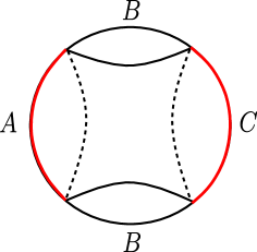
Figure 1: Connected entanglement wedge. How are two subsystems $A$ and $C$ entangled?

Then, how should we understand the quantum entanglement in $\rho_{AC}$? Luckily (or unluckily), there are a plethora of entanglement measures for mixed states with different operational meanings. Several examples are listed below:

1. Entanglement of purification, $E_{P}$ [5]: Considering all the possible purifications $|\psi_{AA^{\prime}CC^{\prime}}\rangle$ of $\rho_{AC}$, it is the minimal entanglement entropy between $AA^{\prime}$ and $CC^{\prime}$:

   $$E_{P}(A:C)=\min_{\Tr_{A^{\prime}C^{\prime}}|(\psi\rangle\langle\psi|)=\rho_{AC}}S_{AA^{\prime}}.$$ (3)

2. Entanglement of formation, $E_{F}$ [6]: Considering all the possible convex decompositions of $\rho_{AC}$ by pure states, $\rho_{AC}=\sum_{i}p_{i}|\psi_{i}\rangle\langle\psi_{i}|$, it is the minimal entanglement entropy of $A$:

   $$E_{F}(A:C)=\inf_{\rho_{AC}=\sum_{i}p_{i}|\psi_{i}\rangle\langle\psi_{i}|}\sum_{i}p_{i}S({\rho_{A}}^{i}),\qquad{\rho_{A}}^{i}=\Tr_{B}(|\psi_{i}\rangle\langle\psi_{i}|).$$ (4)

3. Entanglement cost, $E_{C}$ [7]: This corresponds to entanglement of formation $E_{F}$ in the asymptotic setting:

   $$E_{C}(A:C)=\lim_{m\rightarrow\infty}\frac{E_{F}({\rho_{AC}}^{\otimes m})}{m}.$$ (5)

   Equivalently, it can be also defined as the number of EPR pairs per copy required to create $\rho_{AC}$ with an error vanishing at the asymptotic limit $m\rightarrow\infty$.

4. Squashed entanglement, $E_{sq}$ [8]: Considering all the possible extensions $\rho_{ACE}$ of $\rho_{AC}$, it is the minimum of the conditional mutual information:

   $$E_{sq}(A:C)=\frac{1}{2}\inf_{\Tr_{E}(\rho_{ACE})=\rho_{AC}}I(A:C|E).$$ (6)

5. Distillable entanglement, $E_{D}$ [6, 9]: This is the number of EPR pairs that can be prepared from $\rho_{AC}$ via Local Operations and Classical Communications (LOCCs). It is typically defined in the asymptotic setting:

   $$E_{D}(A:C)=\sup_{r}\left\{r\Big{|}\lim_{m\rightarrow\infty}\Big{[}\inf_{\Lambda\in\text{LOCC}}D\big{(}\Lambda(\rho_{AC}^{\otimes m}),\Phi_{\text{EPR},2^{rm}}\big{)}\Big{]}=0\right\},$$ (7)

   where $D$ represents the trace distance and $\Phi_{\text{EPR},2^{n}}$ represents $n$ EPR pairs, $\quantity(\frac{\ket{00}+\ket{11}}{\sqrt{2}})^{\otimes n}$.

In quantum information theory, these measures are known to obey the following chain of inequalities:

$$\boxed{\ \text{hash}(A:C)\leq E_{D}\leq E_{sq}\leq E_{C}\leq E_{F}\leq E_{P}\leq\min(S_{A},S_{C})\ }$$ (8)

where the hashing lower bound [10, 11, 6], $\text{hash}(A:C)\leq E_{D}(A:C)$, is given by

$$\text{hash}(A:C)\equiv\max(S_{A}-S_{AC},S_{C}-S_{AC},0).$$ (9)

Here, $I_{coh}(A|C)\equiv-S(A|C)=S_{A}-S_{AC}$ is often called the coherent information.

1.1 Previous works

Computing these entanglement measures is challenging in general as involving optimizations over quantum states. Fortunately, in the AdS/CFT correspondence, there is a promising proposal for quantities that involve optimization over all possible purifications (and extensions). These include $E_{P}$ and $E_{sq}$ in the above list [12, 13, 14, 15]. The following hypothesis for purification was shown to hold under physically reasonable assumptions [16].

Hypothesis 1 (Geometric optimization for purification).

In holography, when evaluating entanglement measures involving optimization over all possible purifications, the optimal purification has a semiclassical dual which obeys the RT formula at the leading order in $1/G_{N}$.

To give an insight, let us briefly recall the calculation of $E_{P}$. Given a holographic mixed state $\rho_{AC}$, let $|\Psi_{ACE}\rangle$ be any purification with a semiclassical dual. Since $|\Psi_{ACE}\rangle$ reduces to $\rho_{AC}$, the dual geometry must contain the entanglement wedge of $AC$. Hence, $|\Psi_{ACE}\rangle$ can be constructed by gluing some other geometry at the minimal surface of $AC$, as schematically depicted below for the pure AdS₃:

$$|\Psi_{ACE}\rangle={\begin{array}[]{c}\vbox{\vskip 6.0pt\hbox{\hskip 4.0pt\includegraphics[scale={2.0}]{fig_ACE}}}\end{array}}$$ (11)

where the purifying system $E$ does not necessarily live on asymptotic AdS boundaries. Here one may rely on the state-surface correspondence [17] or invoke the tensor network picture.

Anyhow, it is then immediate to see that $E_{P}$ is given by the entanglement wedge cross section, denoted by $E^{W}$ [14]:

$$\boxed{\ E_{P}(A:C)\approx E^{W}(A:C)\ }$$ (12)

at the leading order in $1/G_{N}$. This can be seen as follows. When $A,C$ have connected wedge, $E^{W}$ is defined by

$$E^{W}(A:C)\equiv\min_{\Sigma_{A:C}}\frac{\text{Area}(\Sigma_{A:C})}{4G_{N}}=\frac{1}{4G_{N}}\ {\begin{array}[]{c}\vbox{\vskip 6.0pt\hbox{\hskip 4.0pt\includegraphics[scale={2.0}]{fig_cross_section}}}\end{array}}$$ (14)

where the minimization is over all possible cross sections $\Sigma_{A:C}$ that splits the connected entanglement wedge of $AC$. Here, we depicted the minimal cross section schematically for the pure AdS₃. When $A,C$ have a disconnected wedge, we have $E^{W}(A:C)=0$ as the entanglement wedge of $AC$ is already separated, suggesting that $A$ and $C$ can be individually purified.

One then notices that the optimal purification is given by choosing $E$ as the minimal surface of $AC$ and splitting $E$ into $A^{\prime}$ and $C^{\prime}$ with respect to the minimal cross section $\Sigma_{A:C}$, as schematically depicted below:

$$|\Psi_{ACE}\rangle={\begin{array}[]{c}\vbox{\vskip 6.0pt\hbox{\hskip 4.0pt\includegraphics[scale={2.0}]{fig_ent_purification}}}\end{array}},\qquad E=A^{\prime}C^{\prime}.$$ (16)

It is straightforward to generalize the above argument to arbitrary dimensions with arbitrary choices of boundary subsystems $A,C$. Since $E^{W}(A:C)$ plays essential roles throughout this paper, we list additional examples of minimal cross sections $\Sigma_{A:C}$ in Fig. 2 for the AdS₃/CFT₂.

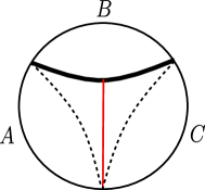
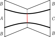
a)          b)    
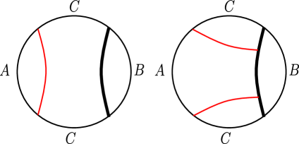
c)          d)    

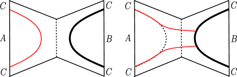
Figure 2: Examples of the minimal cross section $\Sigma_{A:C}$ (shown in red lines). Thick lines represent the boundaries of the entanglement wedge $\mathcal{E}_{AC}$. a,b) Pure AdS₃. c,d) Two-sided BTZ black hole. Note that b) and d) have two candidate cross sections.

Along a similar line of argument, it was shown $E_{sq}\approx\frac{1}{2}I(A:C)$ at the leading order, see [16, 12, 15]. Summarizing these, we have

$$\boxed{\ \text{hash}(A:C)\leq E_{D}\leq\frac{1}{2}I(A:C)\leq E_{C}\leq E_{F}\leq E^{W}(A:C)\ }$$ (17)

under the geometric optimization hypothesis for purification. This greatly bound entanglement measures, but still leaves large margins for $E_{D},E_{C},E_{F}$ in some cases.

1.2 Main claims: Entanglement distillation

In this paper, we are primarily interested in distillable entanglement $E_{D}(A:C)$, the number of EPR pairs that can be prepared via LOCCs. Entanglement distillation is conventionally studied in the asymptotic setting where $m$ copies of $\rho_{AC}$ are given with LOCCs applied jointly on ${\rho_{AC}}^{\otimes m}$ and the distillation rate per copy is considered at the $m\rightarrow\infty$ limit. Here, we will instead focus on one-shot distillable entanglement $E_{D}^{(1)}(A:C)$ which corresponds to the number of (approximate) EPR pairs that can be prepared from a single copy of $\rho_{AC}$ via LOCCs.

Formally, this needs to be defined with some small tolerance $\epsilon$ as follows

$$E_{D}^{(1)}(A:C)\equiv\sup_{r}\left\{r\Big{|}\inf_{\Lambda\in\text{LOCC}}D\big{(}\Sigma(\rho_{AC}),\Phi_{\text{EPR},2^{r}}\big{)}\leq\epsilon\right\}.$$ (18)

In this paper, we will require that

$$\epsilon\rightarrow 0\qquad\mbox{for}\quad 1/G_{N}\rightarrow\infty$$ (19)

or more specifically, $\epsilon\lesssim\text{Poly}(G_{N})$. This condition might look stronger than it should be, but this allows us to obtain some rigorous results.

It will be useful to further highlight the difference between $E_{D}^{(1)}$ and $E_{D}$. Recall that, in the asymptotic setting, we conventionally demand that $\epsilon\rightarrow 0$ as the number of copies $m$ goes to infinity. Instead, here we only have a single copy of $\rho_{AC}$ and thus demand that $\epsilon\rightarrow 0$ as $1/G_{N}\rightarrow\infty$ by tuning a parameter in a theory. Note that the effective number of DOFs in holographic CFTs grows as $1/G_{N}\rightarrow\infty$. In this sense, we are taking an “asymptotic” limit within a single copy system by making the total effective Hilbert space larger. We think that this characterization of distillable entanglement $E_{D}^{(1)}(A:C)$ with the $G_{N}\rightarrow 0$ (or $n\rightarrow\infty$) limit is a more suitable entanglement measure for studying quantum gravity and other related strongly interacting many-body quantum systems.

Another crucial consideration is the use of CC (classical communication). Although CC is conventionally assumed to be freely available in quantum information theory, the use of CC for spacelike separated subsystems in holography is not immediately justified. Hence, we will also consider LO-distillable entanglement where LO (local operation) refers to quantum channels that act locally on $A$ and $C$ without sharing CCs. Note that a quantum channel can be also thought of as a unitary operator acting on the system and ancilla qubits with trace operations.

To summarize, main objects of our study are one-shot LOCC-distillable entanglement and one-shot LO-distillable entanglement, denoted by

$$\begin{split}&E_{D}^{[\text{LOCC}]}(A:C):\text{one-shot distillable EPR pairs from $\rho_{AC}$ via LOCCs}\\ &E_{D}^{[\text{LO}]}(A:C):\text{one-shot distillable EPR pairs from $\rho_{AC}$ via LOs}\end{split}$$ (20)

where the superscript ⁽¹⁾ for one-shot setting is omitted in order to avoid the cluttering of notations. Unless otherwise noted, we will henceforth use $E_{D}^{[\text{LOCC}]}$ and $E_{D}^{[\text{LO}]}$ in a one-shot sense. We will also consider $E_{D}^{[\text{LU}]}(A:C)$ where LO is restricted to local unitary (LU).

The central goal of the present paper is to study $E_{D}^{[\text{LOCC}]}(A:C)$ and $E_{D}^{[\text{LO}]}(A:C)$ for a mixed hologrphic state $\rho_{AC}$ with a connected entanglement wedge. Previously, $E_{D}^{[\text{LOCC}]}(A:C)$ has been studied in the literature when $|\psi_{AC}\rangle$ is a pure state (i.e. $B=\emptyset$) [18]. It is well known that, in an asymptotic (many-copy) setting, $E_{D}^{[\text{LOCC}]}(A:C)$ for pure $|\psi_{AC}\rangle$ is given by

$$E_{D}^{[\text{LOCC(asympt)}]}(A:C)=S_{A}.$$ (21)

For a holographic pure state $|\psi_{AC}\rangle$ in a one-shot setting, it has been found that

$$E_{D}^{[\text{LOCC($1$)}]}(A:C)=S_{A}+O\quantity(\frac{1}{\sqrt{G_{N}}})$$ (22)

where it matches with entanglement entropy $S_{A}$ at the leading order in $1/G_{N}$. Note that Eq. (22) is a relation that holds specifically for holographic states due to their particular spectral properties, and is not true for generic pure states.

LO-distillable entanglement

Let us begin with (one-shot) LO-distillable entanglement $E_{D}^{[\text{LO}]}$. We claim

$$\boxed{\ E_{D}^{[\text{LO}]}(A:C)\approx 0\ \ \ \text{if minimal surfaces $\gamma_{A},\gamma_{C}$ of $A,C$ are separated in the bulk}\ }$$ (23)

at the leading order in $1/G_{N}$. By “separated in the bulk”, we mean that the minimal separation between $\gamma_{A}$ and $\gamma_{C}$, measured in the proper length, is much larger than the Planck length (Fig. 3). We will support this claim by presenting an analytical argument and a holographic argument.

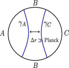
Figure 3: EPR pairs cannot be LO-distilled when minimal surfaces are well separated in the bulk.

Our claim applies to the cases where $A$ and $C$ have connected wedge (i.e. $I(A:C)=O(1/G_{N})$). For instance, in the setup of Fig. 1, no EPR pair can be LO-distilled at the leading order unless $B$ is small enough so that $\gamma_{A}$ and $\gamma_{C}$ approach Planck-scale close to each other. This conclusion is in contrast to the previous claim, often called the mostly bipartite conjecture [19, 20], which proposed that the leading order entanglement in $\rho_{AC}$ would result from $\approx\frac{1}{2}I(A:C)$ copies of unitarily rotated EPR pairs. Note that it has been already argued that correlations in $\rho_{AC}$ must contain genuinely multipartite entanglement [4], refuting the aforementioned conjecture. Here, we essentially claim that entanglement in $\rho_{AC}$ is mostly non-bipartite.

We do, however, believe that EPR pairs can be LO-distilled if the separation between minimal surfaces $\gamma_{A},\gamma_{C}$ becomes order of the Planck scale. Namely, we propose

$$\boxed{\ E_{D}^{[\text{LO}]}(A:C)\approx\frac{1}{4G_{N}}\text{Area}(\gamma_{A}\cap\gamma_{C})\ \ \ \text{if $\gamma_{A},\gamma_{C}$ have overlap}\ }$$ (24)

Here, $\gamma_{A}\cap\gamma_{C}$ refers to the portion of $\gamma_{A}$ and $\gamma_{C}$ that are Planck-scale close to each other. We will support this claim by showing that the Petz recovery map distills EPR pairs along the overlapping portion $\gamma_{A}\cap\gamma_{C}$ in random tensor networks. However, we hasten to emphasize that this relation (Eq. (24)) should be thought of as a heuristic proposal, not a quantitative formula, due to the ambiguity in defining $\gamma_{A}\cap\gamma_{C}$.

The simplest setup with overlapping minimal surfaces is the case where $B$ is empty (i.e. $\rho_{AC}$ is pure) and thus $E_{D}^{[\text{LO}]}(A:C)\approx S_{A}=S_{C}$. A more non-trivial setup is the case where $A$ and $B$ have a disconnected wedge, and thus $\gamma_{A}\subset\gamma_{C}$ as shown in Fig. 4(a). In this case, $A$ is decoupled from $B$ and is instead exclusively entangled with $C$, suggesting $E_{D}^{[\text{LO}]}(A:C)\approx S_{A}$. Another interesting situation is the two-sided AdS black hole where $A$ and $C$ are boundary subsystems on opposite sides (Fig. 4(b)). Namely, when the sizes of $A,C$ are sufficiently large, minimal surfaces $\gamma_{A},\gamma_{C}$ are separated only at (or less than) the Planck scale. Note that when the sizes of $A,C$ are barely large enough to have a connected wedge, $\gamma_{A},\gamma_{C}$ are separated at the AdS scale. For almost overlapping minimal surfaces, we need to take even larger $A,C$. See [21].

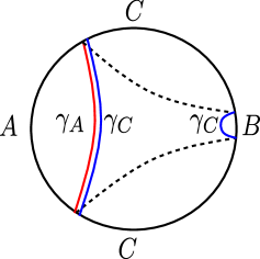
a)          b)    

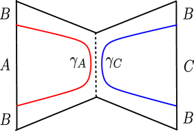
Figure 4: Examples of overlapping minimal surfaces. a) When $A,B$ have disconnected wedge, $\gamma_{A}$ is fully included in $\gamma_{C}$. b) When $A,C$ are large, $\gamma_{A},\gamma_{C}$ may approach Planck-scale close to the horizon.

LOCC-distillable entanglement

Next, we discuss LOCC-distillable entanglement $E_{D}^{[\text{LOCC}]}$. We will focus on a particular subset of LOCCs which we shall call gravitational-LOCCs (denoted as G-LOCCs). The essential difference between LO and LOCC is that the latter may perform measurements. Let us begin by elucidating the class of projective measurements we will employ in G-LOCCs. Recall that degrees of freedom (DOFs) inside an entanglement wedge $\mathcal{E}_{A}$ can be reconstructed on a boundary subsystem $A$, a statement well known as entanglement wedge reconstruction. This implies that, in principle, one can place physical objects similar to an End-of-the-World (EoW) brane inside $\mathcal{E}_{A}$ by some quantum operation acting locally on $A$. Here, EoW brane-like objects terminate the geometry in the bulk. Namely, they do not make further geometric contributions to entanglement entropy, and the RT surface may terminate on EoW brane-like objects [22, 23].

This prompts us to consider the following class of projective measurements which we shall call holographic measurements.

Hypothesis 2 (EoW brane and holographic measurement).

Given a boundary subsystem $A$ and its entanglement wedge $\mathcal{E}_{A}$, let $\Sigma$ be an arbitrary convex surface homologous to $A$. There exists a projective measurement basis on $A$ whose post-measurement states almost surely have a semiclassical dual with an EoW brane-like object placed on a portion of $\Sigma$.

A useful intuition can be obtained in the tensor network picture [27, 28, 29, 30, 24] (Fig. 5). By coarse-graining the state in the radial direction, one can perform projective measurements on DOFs associated with a convex surface $\Sigma$ inside $\mathcal{E}_{A}$. Measuring them in the product basis creates post-measurement states that obey the RT formula with EoW brane(-like objects) placed along the measured portion of $\Sigma$. Furthermore, post-measurement states are expected to have the same geometry regardless of measurement outcomes, with a probability approaching to unity with a vanishing error at the $G_{N}\rightarrow 0$ limit. Namely, the probability amplitude for measuring drastically different geometry (non-saddle states) will be exponentially suppressed with respect to $1/G_{N}$.

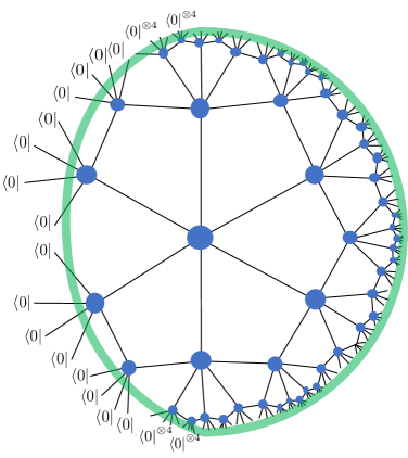
Figure 5: Tensor network picture for placing EoW brane-like object by projective measurement in disentangled basis states.

G-LOCCs are a subset of LOCCs where POVMs are restricted to holographic measurements and CCs are restricted to one round. A more precise definition of G-LOCCs will be presented in Section 4. Focusing on G-LOCCs, we claim

$$\boxed{\ E_{D}^{[\text{G-LOCC}]}(A:C)\approx J^{W}(A:C)\equiv\max\big{(}J^{W}(A|C),J^{W}(C|A)\big{)}.\ }$$ (25)

Here, $J^{W}(A|C)$ is defined by

$$J^{W}(A|C)\equiv S_{A}-E^{W}(A:B)\geq 0$$ (26)

which can be shown to be non-negative. It is useful to schematically depict $J^{W}(A|C)$ for the pure AdS₃:

$$J^{W}(A|C)=\frac{1}{4G_{N}}\max\quantity({\begin{array}[]{c}\vbox{\vskip 4.5pt\hbox{\hskip 3.0pt\includegraphics[scale={1.5}]{fig_SA}}}\end{array}}-{\begin{array}[]{c}\vbox{\vskip 4.5pt\hbox{\hskip 3.0pt\includegraphics[scale={1.5}]{fig_EWAB}}}\end{array}}\,,\quad 0)$$ (29)

It is worth emphasizing that $J^{W}(A:C)\equiv\max(J^{W}(A|C),J^{W}(C|A))$ can be larger than ${\text{hash}(A:C)}\equiv\max(S_{A}-S_{AC},S_{C}-S_{AC},0)$ in some cases.

As a consistency check, recall that $E^{W}(A:B)=0$ if $A$ and $B$ have disconnected wedges. Our proposal predicts that $J^{W}(A|C)=S_{A}$ EPR pairs can be distilled. This is indeed the case since $A$ is decoupled from $B$ due to the disconnected wedges, and is exclusively entangled with $C$.

We will support this claim by presenting an explicit LOCC protocol that distills $J^{W}(A|C)$ EPR pairs. In a nutshell, our protocol performs holographic measurements on $C$ such that the post-measurement state has a semiclassical dual with EoW brane-like objects placed on a portion of minimal surface $\gamma_{C}$. Namely, $\gamma_{A}$ can change its profile due to projective measurements such that $\gamma_{A}$ overlaps with $\gamma_{C}$, enabling entanglement distillation from the post-measurement $\rho_{AC}$.

The remaining task is to show the optimality of this protocol at the leading order. We argue this by relating $J^{W}(A|C)$ to another entanglement measure, often called locally accessible information [31, 32, 33].

1. Locally accessible information, $J(A|C)$: Considering all the possible measurements described by positive operator-valued measures (POVMs) $\{\Pi^{i}_{C}\}$ acting on $C$ and resulting marginal states $\{p_{j},\rho_{A}^{j}\}$, it is the maximal possible entropy drop $\Delta S_{A}$, on average, by POVMs on $C$

   $$J(A|C) \equiv S_{A}-\min_{\{\Pi^{i}_{C}\}_{i}}\sum_{j}p_{j}S_{A}(\rho_{A}^{j}),\qquad p_{j}=\Tr(\Pi^{j}_{C}\rho_{C})$$ (30)

   $$=\max_{\{\Pi^{i}_{C}\}_{i}}\sum_{j}p_{j}S(\rho_{A}^{j}||\rho_{A}),$$ (31)

   where $S(\rho||\sigma)=\Tr(\rho\log\rho-\rho\log\sigma)$ is a quantum relative entropy.

Computing $J(A|C)$ is challenging in general as involving optimizations over decompositions of $\rho_{AC}$ in POVM basis states. Here, by focusing on holographic measurements that place EoW brane-like objects, one can consider gravitational locally accessible information.

1. Gravitational locally accessible information, $J^{G}(A|C)$: Considering all the possible holographic measurements $\{\Pi^{i}_{C}\}$ which place EoW brane-like objects and resulting marginal states $\{p_{j},\rho_{A}^{j}\}$, it is the maximal possible entropy drop $\Delta S_{A}$, on average, by holographic measurements on $C$

   $$J^{G}(A|C) \equiv S_{A}-\min_{\{\Pi^{i}_{C}\}_{i}\in\text{holographic}}\sum_{j}p_{j}S_{A}(\rho_{A}^{j}),\qquad p_{j}=\Tr(\Pi^{j}_{C}\rho_{C})$$ (32)

   $$=\max_{\{\Pi^{i}_{C}\}_{i}\in\text{holographic}}\sum_{j}p_{j}S(\rho_{A}^{j}||\rho_{A}).$$ (33)

With this restriction, it is then immediate to see

$$\boxed{\ J^{G}(A|C)\approx J^{W}(A|C)\equiv S_{A}-E^{W}(A:B)\ }$$ (34)

at the leading order in $1/G_{N}$. Indeed, placing EoW brane-like objects on $\gamma_{C}$ achieves the entropy drop of $\Delta S_{A}=J^{W}(A|C)$, as schematically shown below for the pure AdS₃

$$S_{A}^{\text{before}}=\frac{1}{4G_{N}}{\begin{array}[]{c}\vbox{\vskip 4.5pt\hbox{\hskip 3.0pt\includegraphics[scale={1.5}]{fig_SA}}}\end{array}}\,,\qquad S_{A}^{\text{after}}=\frac{1}{4G_{N}}{\begin{array}[]{c}\vbox{\vskip 4.5pt\hbox{\hskip 3.0pt\includegraphics[scale={1.5}]{fig_EWAB}}}\end{array}}$$ (37)

where $S_{A}^{\text{after}}$ is evaluated in the presence of EoW brane-like objects. Note that post-measurement states almost surely have the same geometry regardless of measurement outcomes.

Subleading effects

Our claims so far can be summarized as follows

$$E_{D}^{[\text{LO}]}(A:C)\approx 0,\qquad E_{D}^{[\text{G-LOCC}]}(A:C)\approx J^{W}(A:C)$$ (38)

at the leading order in $1/G_{N}$ when $\gamma_{A},\gamma_{C}$ are well separated in the bulk. We however believe that subleading corrections to the above claims do exist. Namely, we identify three possible physical mechanisms for subleading effects.

1. Traversable wormhole: An LOCC version of traversable wormhole protocol distills EPR pairs from $\rho_{AC}$ when $A,C$ are sufficiently large subsystems on two boundaries. This may potentially distill subleading EPR pairs even in a regime with $J^{W}(A:C)=0$.

2. Holographic scattering: That the bulk scattering process necessitates the connected entanglement wedge may suggest the possibility of LOCC-distillability from $\rho_{AC}$ at the subleading order even in a regime with $J^{W}(A:C)=0$.

3. Planck-scale effect: $E_{D}^{[\text{LO}]}(A:C)$ will receive significant corrections when $\gamma_{A},\gamma_{C}$ are Planck-scale close to each other.

Entanglement of formation

We have argued that $J^{G}(A|C)\approx J^{W}(A|C)$ when POVMs are restricted to holographic measurements that place EoW brane-like objects. A naturally arising question concerns whether generic POVMs may achieve further entropy drop on average. We will present some physical arguments suggesting that holographic measurements are nearly optimal at the leading order, namely

$$\boxed{\ J(A|C)\stackrel{{\scriptstyle?}}{{\approx}}J^{G}(A|C)\approx J^{W}(A|C),\ }$$ (39)

based on the generalized RT formula and the bulk causality.

This proposal ($J(A|C)\approx J^{W}(A|C)$) has a parallel statement for entanglement of formation $E_{F}(A:B)$ for a tripartite quantum state $|\psi_{ABC}\rangle$. Recall that, considering all the possible decompositions of $\rho_{AB}$ by pure states, $\rho_{AB}=\sum_{i}p_{i}|\psi_{i}\rangle\langle\psi_{i}|_{AB}$, entanglement of formation $E_{F}(A:B)$ is given by the minimum of $\sum_{i}p_{i}S({\rho_{A}}^{i})$. Here, it is known that $E_{F}(A:B)$ is related to locally accessible information $J(A|C)$ by the Koashi-Winter relation [34]:

$$\boxed{\ J(A|C)=S_{A}-E_{F}(A:B).\ }$$ (40)

Recalling the proposal of $J(A|C)\approx J^{W}(A|C)\equiv S_{A}-E_{W}(A:B)$, this suggests

$$\boxed{\ E_{F}(A:B)\approx E^{W}(A:B)\ }$$ (41)

at the leading order in $1/G_{N}$.

1.3 Connected wedge vs. Locally accessible information

One important implication of our claims is that the connected entanglement wedge does not necessarily imply distillable entanglement under G-LOCCs. Let us focus on the pure AdS₃ and think of increasing the sizes of $A,C$ while keeping the arrangement of $A,C$ symmetric (see Fig. 6).

1. When $A$ and $C$ occupy less than quarters of the whole system, the entanglement wedge of $AC$ is disconnected with $I(A:C)\approx 0$, and we have $E_{D}^{[\text{LO}]},E_{D}^{[\text{G-LOCC}]}\approx 0$ at the leading order.

2. When $A$ and $C$ occupy slightly more than quarters, the entanglement wedge of $AC$ will be connected with $I(A:C)\sim O(1/G_{N})$, but $J^{W}(A|C),J^{W}(C|A)\approx 0$, and thus $E_{D}^{[\text{LO}]},E_{D}^{[\text{G-LOCC}]}\approx 0$ at the leading order.

3. When $A$ and $C$ occupy much more than quarters, $J^{W}(A:C)\sim O(1/G_{N})$, and one can distill $E_{D}^{[\text{G-LOCC}]}(A:C)\approx J^{W}(A|C)$ EPR pairs at the leading order. However, $E_{D}^{[\text{G-LOCC}]}(A:C)$ remains smaller than $\frac{1}{2}I(A:C)$.

4. When $B$ becomes empty and $\gamma_{A},\gamma_{C}$ overlap, we have $E_{D}^{[\text{LO}]},E_{D}^{[\text{G-LOCC}]},\frac{1}{2}I(A:C)\approx S_{A}$ at the leading order.

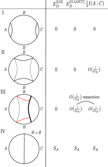
a)   b)  

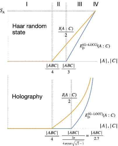
Figure 6: a) Summary of our claims on $E_{D}^{[\text{LO}]},E_{D}^{[\text{G-LOCC}]},\frac{1}{2}I(A:C)$. b) $E_{D}^{[\text{G-LOCC}]}(A:C)$ vs. $\frac{1}{2}I(A:C)$. In holography, we define $|X|$ as the length of a boundary subsystem $X$ divided by the entire length of the circle.

These observations are schematically depicted in Fig. 6(b), highlighting the dichotomy between $E_{D}^{[\text{G-LOCC}]}(A:C)$ and $\frac{1}{2}I(A:C)$. In quantum information theory, entangled states that are not distillable are often called bound entangled states [35]. Our results suggest that holographic states with connected entanglement wedge, but with $J^{W}(A:C)=0$, are examples of bound entangled states in the following sense:

$$E_{D}^{[\text{LO}]}(A:C),E_{D}^{[\text{G-LOCC}]}(A:C)\approx 0<\frac{1}{2}I(A:C)\lesssim E_{F}(A:C)$$ (42)

in one-shot settings.

Leading vs. subleading contribution

Throughout the paper, we will discuss leading vs. subleading order contributions to distillable entanglement and other related entanglement measures. In the context of Haar random states, the leading order contributions will be expressed by $O(n)$, indicating that the corresponding quantity grows linearly in $n$ at the limit of large $n$. In the context of holography, the leading order contributions will be expressed by $O(1/G_{N})$ at the limit of $G_{N}\rightarrow 0$. Subleading contributions are those which grow slower than linear in $n$ or $1/G_{N}$, and will be expressed by $o(n)$ or $o(1/G_{N})$. Furthermore, we will use the notation “$f\approx g$” to indicate that $f$ equals $g$ at the leading order, namely $|f-g|\sim o(n),o(1/G_{N})$.

In full holography, subleading contributions often scale polynomially as $\sim O(1/G_{N}^{1-a})$ with some constant $0<a<1$. For Haar random states and random tensor networks, subleading contributions are often even smaller with exponential suppression with respect to $n$, which will be expressed as $o(1)$. It is important to note that subleading contributions can be divergent or finite, depending on the systems of interest, setups, and entanglement measures.

One potential source of subleading contributions is entanglement in bulk matter fields. Throughout the paper (except some part of Section 3), we will assume that bulk matter fields carry subleading $\sim o(1/G_{N})$ entropy and thus make only subleading contributions to distillable entanglement. This assumption is imposed mostly in order to avoid backreaction to the geometry from matter fields. Namely, we will take a perspective that, when a $O(1/G_{N})$ bulk entropic contribution exists, a semiclassical picture becomes invalid.

In fact, we expect that the bulk contribution to distillable entanglement $E_{D}(A:C)$ will remain negligibly small. Namely, we think that this expectation may be justified even without assuming bulk entropy to be subleading. This is due to that we are particularly interested in regimes where minimal surfaces $\gamma_{A}$ and $\gamma_{C}$ are spatially separated, at the order of the AdS scale. Observe that distributing an EPR pair between two entanglement wedges $\mathcal{E}_{A}$ and $\mathcal{E}_{C}$ will add EPR-like entanglement to $\rho_{AC}$ on the boundary. In the bulk low energy effective field theory, however, we generally expect that two spatially disconnected subregions have quantum correlations that delay exponentially with respect to the spatial separation (except for highly fine-tuned configurations). This suggests that bulk entanglement between two entanglement wedges $\mathcal{E}_{A}$ and $\mathcal{E}_{C}$ will be negligibly small, and as such, bulk matter fields will not make significant contributions to distillable entanglement in $\rho_{AC}$.

Throughout the paper, we will take a perspective that $\text{Area}(\gamma)$ of some surface $\gamma$ is given exactly by the value of the classical area. Thus, our interpretation is that entropic quantities and entanglement measures receive subleading corrections whereas the leading order contributions are given by classical areas. Instead, one may take a perspective that $\text{Area}(\gamma)$ is a quantum operator and thus its expectation value contains subleading contributions by design.

Finally, we briefly comment on UV divergence. While entanglement entropy $S_{A}$ for a subsystem is UV divergent, the mutual information $I(A:C)$ for spatially disjoint subsystems $A,C$ is UV finite as it computes the area difference where UV divergences cancel with each other. Since $E_{D}(A:C)$ is upper bounded by $\frac{1}{2}I(A:C)$, $E_{D}(A:C)$ will also be UV finite. A similar observation holds for (gravitational) locally accessible information $J^{G}(A|C)$ which will be UV finite, thanks to its rewritten form as relative entropy (Eq. (33)). One limitation of our work is that we always assume, either explicitly or implicitly, the existence of some local basis with nicely factorized DOFs (i.e. qubits). Despite this caveat, the above considerations on UV divergences (and rewriting of $J^{W}(A|C)$ as relative entropy) suggest that our arguments may apply to continuum theories (e.g. those described by type-III von Neumann algebra) as well.

Plan of the paper

This paper is organized as follows.

• In Section 2, we discuss entanglement distillation for Haar random states and illustrate holographic interpretations.

  We will begin by presenting simple counting arguments showing $E_{D}^{[\text{LO}]}(A:C)\approx 0$ for $n_{A},n_{B},n_{C}<\frac{n}{2}$. We also present a rigorous bound by using the fact that the Petz recovery map is a “pretty good” decoder. Although this argument is more rigorous than the counting argument, this only shows $E_{D}^{[\text{LO}]}(A:C)\lesssim\min(\max(n_{A}-n_{B},0),\max(n_{C}-n_{B},0))$. Finally, we present an explicit LOCC protocol that distills $\approx\text{hash}(A:C)$ EPR pairs.

• In Section 3, we discuss LO-distillation for holography by mostly focusing on random tensor networks.

  We will offer a physical argument behind our proposal, $E_{D}^{[\text{LO}]}(A:C)\approx 0$, by interpreting entanglement wedge reconstruction as LO entanglement distillation. Namely, we argue that our proposal follows from the assumption that DOFs behind the entanglement wedge $\mathcal{E}_{R}$ of some subsystem $R$ cannot be reconstructed on $R$. Also, by studying the performance of the Petz recovery map, we obtain a rigorous bound $E_{D}^{[\text{LO}]}(A:C)\lesssim\min(J^{W}(A|C),J^{W}(C|A))$ for random tensor networks. This proves the existence of a regime where $E_{D}^{[\text{LO}]}(A:C)\approx 0$ but $E_{D}^{[\text{LOCC}]}(A:C)\sim O(1/G_{N})$.

• In Section 4, we discuss G-LOCC distillation for holography.

  We will begin by presenting a G-LOCC protocol that distills $\approx J^{W}(A:C)$ EPR pairs. We then show that (gravitational) locally accessible information is given by $J^{G}(A|C)\approx J^{W}(A|C)$. Finally, we show that this protocol is optimal under G-LOCC protocols, and thus $E_{D}^{[\text{G-LOCC}]}(A:C)\approx J^{W}(A:C)$.

• In Section 5, we discuss possible physical mechanisms for subleading corrections to our proposals of $E_{D}^{[\text{LO}]}(A:C)\approx 0$ and $E_{D}^{[\text{G-LOCC}]}(A:C)\approx J^{W}(A:C)$.

• In Section 6, we discuss whether LOCCs may outperform G-LOCCs in entanglement distillation or not. Specifically, we will provide some physical arguments, based on the bulk causality and the generalized RT formula, suggesting $J^{G}(A|C)\approx J(A|C)$, and as a result, $E_{D}^{[\text{1WAY LOCC}]}(A:C)\approx J^{W}(A:C)$.

• In Section 7, we relate our findings to entanglement of formation $E_{F}$ by using the Koashi-Winter relation and propose that $E_{F}(A:C)\approx E^{W}(A:C)$. We also comment on a previous no-go argument by Umemoto and how our proposal avoids it.

• In Section 8, we argue that holographic states serve as examples of bound entangled states in one-shot settings in a sense that $\frac{1}{2}I(A:C)\sim O(1/G_{N})$, but $E_{D}^{[\text{G-LOCC}]}(A:C)\approx 0$. We will also remark on a certain previous proposal concerning holographic bound states and point out a potential loophole in the argument.

• In Section 9, we conclude with discussions and future problems.

• In Appendix A, we present an explicit calculation of $J^{W}(A:C)$ in the pure AdS₃. Namely, we will identify the critical angle $\theta_{\ast}$ above which $J^{W}(A:C)\sim O(1/G_{N})$ in the cases when $A$ and $C$ are symmetrically placed.

• In Appendix B, we present an explicit calculation of $J^{W}(A:C)$ in a two-sided BTZ black hole where $A$ and $C$ are symmetrically placed on two opposite sides.

• In Appendix C, we study entanglement properties of $\rho_{AA^{\prime}}$ in the double-copy state constructed from a Haar random state.

• In Appendix D, we study entanglement properties of $\rho_{AA^{\prime}}$ in the double-copy state constructed from a random tensor network.

2 Entanglement distillation in Haar random state

A Haar random state serves as a minimal toy model of holography as its entanglement entropies satisfy the RT-like formula at the leading order with respect to the number of qubits. In this section, we discuss entanglement distillation problems in Haar random states.

Our central claim is that $E_{D}^{[\text{LO}]}(A:C)\approx 0$ at the leading order in $n$ when each subsystem $A,B,C$ occupies less than half of the whole system. Specifically, we will consider the large $n$ limit where $\frac{n_{A}}{n},\frac{n_{B}}{n},\frac{n_{C}}{n}<\frac{1}{2}$ are held constant. We will offer holographic interpretations of this claim, demonstrating that a connected wedge does not necessarily imply distillable entanglement under local operations. We then present a simple physical argument for $E_{D}^{[\text{LU}]}(A:C)\approx 0$ based on the probability distributions of states in the Hilbert space (where LU stands for local unitaries instead of local operations). We also provide a slightly indirect, yet rigorous, argument which proves $E_{D}^{[\text{LO}]}(A:C)\lesssim\max(0,S_{A}-S_{AC}),\max(0,S_{C}-S_{AC})$ by relying on the decoding performance of the Petz recovery map.

As for LOCC-distillable entanglement, we will begin by presenting an explicit LOCC protocol that distills $\approx\text{hash}(A:C)$ EPR pairs and present a holographic interpretation of the protocol. Namely, we will demonstrate that projective measurements on a subsystem in a random basis can be viewed as placing EoW brane-like objects, and thus can be viewed as an analogue of holographic measurements. Focusing on this particular subset of LOCCs, which we shall later call gravitational LOCC (G-LOCC), one can show that $E_{D}^{[\text{G-LOCC}]}(A:C)\approx\text{hash}(A:C)$ at the leading order in $n$ when each subsystem $A,B,C$ occupies less than a half of the whole system.

2.1 LO-distillable entanglement

We begin by illustrating our claim on $E_{D}^{[\text{LO}]}$ for Haar random states along with its holographic interpretation. Consider an $n$-qubit Haar random state $|\psi_{AB}\rangle$ in a bipartition into $A$ and $B$ with $n_{A}$ and $n_{B}=n-n_{A}$ qubits respectively. We have

$$S_{A}\approx\min(n_{A},n-n_{A})$$ (43)

at the leading order in $n$, due to the result often called Page’s theorem [36, 37, 38]. This well-celebrated result can be interpreted as the RT-like formula with the area (equals the total number of qubits across the cut) minimization by employing tensor diagrams:

$$S_{A}\approx\min\big{(}{\begin{array}[]{c}\vbox{\vskip 6.0pt\hbox{\hskip 4.0pt\includegraphics[scale={2.0}]{fig_Haar_A}}}\end{array}},{\begin{array}[]{c}\vbox{\vskip 6.0pt\hbox{\hskip 4.0pt\includegraphics[scale={2.0}]{fig_Haar_B}}}\end{array}}\big{)}.$$ (46)

Furthermore, assuming $n_{A}<n_{B}$, we see that $A$ is nearly maximally entangled with a $2^{n_{A}}$-dimensional subspace in $B$. This suggests that one can LO-distill $n_{A}$ EPR pairs from $A$ and $B$ by applying some unitary operator $U_{B}$, meaning that $E_{D}^{[\text{LO}]}(A:B)\approx n_{A}$. More precisely, one can distill $\approx n_{A}$ approximate EPR pairs with a vanishing error $\epsilon\rightarrow 0$ at the limit of large $n$. The Petz recovery map achieves this as we will further discuss later. In the holographic interpretation, this LO-distillability can be understood by overlapping minimal surfaces, namely $\gamma_{A}=\gamma_{B}$.

Next, consider a tripartite $n$-qubit Haar random state $|\psi_{ABC}\rangle$ on $A$, $B$, and $C$. Let us first assume that $C$ contains more than half of the system with $n_{C}>\frac{n}{2}$. We then have

$$S_{C}=S_{AB}\approx{\begin{array}[]{c}\vbox{\vskip 6.0pt\hbox{\hskip 4.0pt\includegraphics[scale={2.0}]{fig_Haar_C}}}\end{array}}=n_{A}+n_{B}$$ (48)

which suggests that $A$ and $B$ are nearly fully decoupled from each other, and thus $A$ is nearly maximally entangled with $C$. In this case, there exists a unitary $U_{C}$ that LO-distills EPR pairs between $A$ and $C$ with $E_{D}^{[\text{LO}]}(A:C)\approx n_{A}$. Again, this can be understood as a consequence of overlapping minimal surfaces, as shown in Fig. 7(a). The same argument applies for $n_{A}>\frac{n}{2}$ by exchanging $A$ and $C$.

When $n_{B}>\frac{n}{2}$, $A$ and $C$ are nearly fully decoupled from each other as $I(A:C)\approx 0$. Since the distillable entanglement is bounded by the mutual information from above, we have $E_{D}^{[\text{LO}]}(A:C)\approx 0$.

Finally, when $n_{A},n_{B},n_{C}<\frac{n}{2}$, we have

$$S_{R}\approx n_{R},\qquad R=A,B,C$$ (49)

where the minimal surface $\gamma_{R}$ of any subsystem $R=A,B,C$ does not contain the tensor at the center. This mimics the situation with the connected wedge as in Fig. 1. Namely, by splitting $B$ into two subsystems, we can schematically draw the minimal surface of $AC$ as follows

$$S_{AC}\approx\ {\begin{array}[]{c}\vbox{\vskip 6.0pt\hbox{\hskip 4.0pt\includegraphics[scale={2.0}]{fig_Haar_wedge}}}\end{array}}=n_{B}\qquad I(A:C)\approx n_{A}+n_{C}-n_{B}\sim O(n).$$ (51)

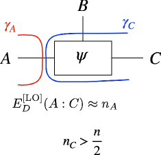
a)          b)    

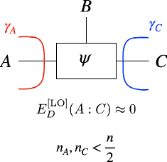
Figure 7: LO-distillable entanglement $E_{D}^{[\text{LO}]}(A:C)$ and minimal surfaces. a) Overlapping minimal surfaces. b) Separated minimal surfaces.

The central question is whether one can LO-distill EPR pairs from $\rho_{AC}$. Observing that minimal surfaces $\gamma_{A},\gamma_{C}$ are separated by the tensor at the center, we claim

$$E_{D}^{[\text{LO}]}(A:C)\approx 0$$ (52)

at the leading order in $n$. See Fig. 7(b) for illustration.

2.2 Atypicality of bipartite entanglement

Here, we present a heuristic argument based on a simple physical observation concerning the probability distribution of states in the Hilbert space. For simplicity of discussion, we shall focus on entanglement distillation by local unitary (LU) operations, instead of generic LOs. The essential difference between LU and LO is whether one allows the use of local ancilla qubits or not. While we do not expect qualitatively different results for LO and LU-distillable entanglement, the argument below does not apply to LO cases. This subsection shows $E_{D}^{[\text{LU}]}(A:C)\approx 0$ when $\frac{n_{A}}{n},\frac{n_{B}}{n},\frac{n_{C}}{n}<\frac{1}{2}$ at large $n$ by simple counting argument.

We begin by presenting a useful insight concerning Haar random states by following [41]. In an $n$-qubit system, there are $2^{n}$ mutually orthogonal states which may be labeled by $|j\rangle$ with $j=1,\cdots,2^{n}$. But if we relax the orthogonality condition, one can show that there are doubly-exponentially ($e^{e^{O(n)}}$) many states that are nearly orthogonal to each other. This can be readily understood by considering the following family of $n$-qubit quantum states

$$|\psi(c)\rangle=\frac{1}{2^{n/2}}(c_{1}|1\rangle+c_{2}|2\rangle+\cdots+c_{2^{n}}|2^{n}\rangle),\quad c_{j}=\pm 1,$$ (53)

where $c=(c_{1},\cdots,c_{2^{n}})$. By choosing $c$ and $c^{\prime}$ randomly, we find

$$|\langle\psi(c)|\psi(c^{\prime})\rangle|=\Big{|}\frac{1}{2^{n}}\sum_{j=1}^{2^{n}}c_{j}c_{j}^{\prime}\Big{|}\approx\frac{1}{2^{n/2}}\underset{n\rightarrow\infty}{\longrightarrow}0.$$ (54)

This suggests that there are at least doubly-exponential, nearly orthogonal quantum states in the Hilbert space.

The upshot of this observation is that choosing a Haar random state is fundamentally akin to picking a state from a set of doubly-exponentially many quantum states that are nearly orthogonal to each other. Although the above observation is not meant to be a rigorous statement, this heuristic characterization of Haar random states can be made rigorous by introducing a tolerance $\epsilon$ in terms of fidelity overlaps, i.e. an $\epsilon$-net. See [42, 43] for instance.

Given a quantum state $|\psi_{ABC}\rangle$ with $n_{A},n_{B},n_{C}<\frac{n}{2}$, suppose that it is possible to distill $n_{AB},n_{BC},n_{CA}$ EPR pairs between two subsystems by applying local unitaries $U_{A}\otimes U_{B}\otimes U_{C}$. This leaves $n^{\prime}=n-2(n_{AB}+n_{BC}+n_{CA})$ qubits decoupled from EPR pairs as shown in Fig. 8. Here, the decoupled $n^{\prime}$-qubit state can be arbitrary.

We now argue that such quantum states with LU-distillable EPR pairs are extremely rare in the Hilbert space. For this purpose, let us denote the total number of nearly orthogonal states with $\sim\epsilon$ mutual overlaps by $\Phi_{\text{state}}(n)$. Precise form of $\Phi_{\text{state}}(n)$ is not significant in the argument below, and we will only need that $\Phi_{\text{state}}(n)$ scales doubly-exponentially. Similarly, there are doubly-exponentially many unitary operators acting on the $n$-qubit Hilbert space, and let us denote the total number by $\Phi_{\text{unitary}}(n)$. Recalling that an $n$-qubit unitary can be viewed as a $2n$-qubit state via the Choi isomorphism, we have

$$\Phi_{\text{unitary}}(n)<\Phi_{\text{state}}(2n).$$ (55)

Figure 8: Tripartite state $|\psi_{ABC}\rangle$ with LU-distillable EPR pairs.

Let us estimate the total number of states with LU-distillable EPR pairs. First, one can unitarily rotate $A,B,C$ by $U_{A}\otimes U_{B}\otimes U_{C}$. The number of such unitary operators is given by

$$\Phi_{\text{unitary}}(n_{A})\Phi_{\text{unitary}}(n_{B})\Phi_{\text{unitary}}(n_{C})<\Phi_{\text{unitary}}(n_{R}+c),\qquad n_{R}=\max\big{(}n_{A},n_{B},n_{C}\big{)}$$ (56)

where $c>0$ is an $O(1)$ constant. The upper bound comes from the fact $\Phi_{\text{unitary}}$ being doubly exponential. Also, the number of decoupled $n^{\prime}$-qubit states is given by $\Phi_{\text{state}}(n^{\prime})$. Hence, the total number of states with LU-distillable EPR pairs is upper bounded by

$$\Phi_{\text{state}}(2n_{R}+c)\Phi_{\text{state}}(n^{\prime})$$ (57)

which is much less than $\Phi_{\text{state}}(n)$ as long as $0\lesssim n_{R}\lesssim\frac{n}{2}$. Hence, by randomly choosing a state from a set of $\Phi_{\text{state}}(n)$ nearly orthogonal states, it is extremely unlikely to obtain a state with LU-distillable entanglement, suggesting $E_{D}^{[\text{LU}]}(A:C)\approx 0$ at the leading order in $n$.

It is worth noting that this argument breaks down when $n^{\prime}\approx n$ (i.e. no EPR pairs) or $2n_{R}\approx n$ (i.e. one subsystem contains more than half of the system). In the latter case, we can indeed perform LU-distillation of EPR pairs as one of the subsystems contains more than half of the whole system.

Although we considered the LU-distillability of perfect EPR pairs in the above analysis, relaxing this condition to admit approximate EPR pairs does not significantly change the analysis. Note that we have defined $E_{D}^{[\text{LO}]}$ in terms of entanglement fidelity as in Eq. (18).

While this counting argument does not generalize to LO cases as adding ancilla qubits spoils the counting argument, we expect that

$$E_{D}^{[\text{LO}]}(A:C)\approx E_{D}^{[\text{LU}]}(A:C)$$ (58)

for Haar random states. Here, we present a brief sketch of the argument supporting Eq. (58). Suppose that a local quantum channel $\mathcal{Q}_{A}\otimes\mathcal{Q}_{C}$ prepares $n_{D}$ (approximate) EPR pairs by acting on $\rho_{AC}$. We may label the output Hilbert spaces as $\mathcal{Q}_{A}:A\rightarrow D$ and $\mathcal{Q}_{C}:C\rightarrow D^{\prime}$ so that $\mathcal{Q}_{A}\otimes\mathcal{Q}_{C}(\rho_{AC})\approx|\text{EPR}\rangle\langle\text{EPR}|_{DD^{\prime}}$. Let us consider the following state

$$\sigma_{AD^{\prime}}\equiv(I_{A}\otimes\mathcal{Q}_{C})(\rho_{AC}).$$ (59)

Since $D^{\prime}$ must be nearly maximally entangled with $A$, we expect that $\sigma_{AD^{\prime}}$ can be viewed as an approximate isometry $\Lambda:D^{\prime}\rightarrow A$ via the Choi isomorphism. We can then construct an inverse $\Lambda^{-1}:A\rightarrow D$ and apply it on $A$ to prepare EPR pairs on $DD^{\prime}$. This will replace $\mathcal{Q}_{A}$ with some unitary $U_{A}$ without the need of adding ancilla qubits. One can repeat the same argument for $\mathcal{Q}_{C}$ to show that LUs are sufficient to prepare $|\text{EPR}\rangle_{DD^{\prime}}$.

2.3 Bound from the Petz map

Next, we provide another argument that utilizes a certain powerful result by Barnum and Knill, concerning entanglement fidelity in quantum error corrections [44]. See [45] for an introduction of this result in the context of holography. Our argument relies on the fact that the Petz recovery map is a pretty good decoder, and thus it suffices to study the decoding performance of the Petz recovery map in discussing LO-distillable entanglement. Unlike the above counting argument, the argument below applies to LO cases as well. However, this provides a weaker upper bound on $E_{D}^{[\text{LO}]}(A:C)$, namely $E_{D}^{[\text{LO}]}(A:C)\lesssim\min(\max(0,S_{A}-S_{AC}),\max(0,S_{C}-S_{AC}))$.

We begin by interpreting LO-distillable entanglement as the decodability in a quantum error correcting code. Recall that, given a Haar random state $|\psi_{ABC}\rangle$, one can view it as a quantum error-correcting code with an approximate encoding isometry $\Lambda:A\rightarrow BC$ via the Choi-Jamiołkowski isomorphism (the state-channel duality) as $\rho_{A}$ can be approximated by the maximally mixed state in trace distance. (See [46] for the introduction of the Choi-Jamiołkowski isomorphism in the context of many-body physics and holography.) Namely, we can write

$$|\psi_{ABC}\rangle\approx\Lambda\otimes I_{A^{\prime}}|\text{EPR}\rangle_{A^{\prime}A}={\begin{array}[]{c}\vbox{\vskip 6.0pt\hbox{\hskip 4.0pt\includegraphics[scale={2.0}]{fig_choi_distill}}}\end{array}}$$ (61)

where $\Lambda$ can be treated as a Haar random isometry and the initial state on $A^{\prime}A$ is chosen to be a canonical purification of $\rho_{A}\approx\frac{I_{A}}{d_{A}}$, namely $|\text{EPR}\rangle_{A^{\prime}A}$. Henceforth, we denote the dimension of a subsystem $X$ containing $n_{X}$ qubits by $d_{X}=2^{n_{X}}$. Below, we will mostly focus on LU-distillable entanglement since generalization to LO-distillable entanglement is straightforward as we will explain later.

Suppose that $n_{A_{0}}$ EPR pairs can be LU-distilled from $\rho_{AC}$ by applying some local unitary operator $U_{A}\otimes U_{C}$. Using the Choi-Jamiołkowski isomorphism, this can be viewed as a decoding problem in a quantum error code as shown in Fig. 9 where EPR pairs are to be prepared on $A_{0}$ and $A_{0}^{\prime}$. Specifically, we have the following processes:

1. Encoding: An isometry $\Theta:A_{0}^{\prime}\rightarrow A_{1}BC$ encodes an $n_{A_{0}}$-qubit input state into an $(n_{A_{1}}+n_{B}+n_{C})$-qubit output state.

2. Noise: The system undergoes an erasure noise channel $\mathcal{T}(\cdot)=\Tr_{A_{1}B}(\cdot)$.

3. Decoding: A decoding channel $\mathcal{D}:C\rightarrow A_{0}^{\prime}$ is applied on $C$ to generate EPR pairs on $A_{0}^{\prime}A_{0}$.

In this interpretation, the average decoding success can be quantified by the entanglement fidelity which is defined by

$$F_{\mathcal{D}}\equiv\langle\text{EPR}_{A_{0}A_{0}^{\prime}}|\mathcal{I}_{A_{0}}\otimes\mathcal{D}_{C\rightarrow A_{0}^{\prime}}(\rho_{A_{0}C})|\text{EPR}_{A_{0}A^{\prime}_{0}}\rangle.$$ (62)

If (approximate) EPR pairs can be prepared on $A_{0}A_{0}^{\prime}$, we would have $F_{\mathcal{D}}\geq 1-\epsilon$ with some $\epsilon\rightarrow 0$ as $n\rightarrow\infty$. (Recall Eq. (19).) Below, we will prove that such $\epsilon$ cannot exist for $n_{A_{0}}\gtrsim\max(0,n_{A}-n_{B})$, suggesting $E_{D}^{[\text{LU}]}(A:C)\lesssim\max(0,n_{A}-n_{B})$.

In [44], Barnum and Knill showed that the following inequality holds for any decoder $\mathcal{D}$:

$$\boxed{\ F_{\mathcal{D}_{\text{Petz}}}\geq F_{\mathcal{D}}^{2}\ }$$ (63)

where $\mathcal{D}_{\text{Petz}}$ denotes the Petz recovery map

$$\mathcal{D}_{\text{Petz}}(\cdot)\equiv\rho^{1/2}\mathcal{N}^{\dagger}\big{[}\mathcal{N}(\rho)^{-1/2}(\cdot)\mathcal{N}(\rho)^{-1/2}\big{]}\rho^{1/2}.$$ (64)

Here $\mathcal{N}$ is a quantum channel representing both encoding and noise ($\mathcal{N}=\mathcal{T}\circ\Theta$ in our setup). Also, $\rho$ denotes the reference state which is $\rho_{A_{0}}\approx\frac{I_{A_{0}}}{d_{A_{0}}}$ in our setting. The upshot of this result is that, if there exists a good decoder $\mathcal{D}$ which distills EPR pairs with high fidelity, then the Petz map will also distill EPR pairs with reasonably high fidelity. Namely, if $F_{\mathcal{D}}=1-\epsilon$ with small $\epsilon$ for some $\mathcal{D}$, we can show $F_{\mathcal{D}_{\text{Petz}}}\geq 1-2\epsilon+O(\epsilon^{2})$. In other words, the Petz map is a pretty good (if not the best) decoder. Hence, as long as one knows that entanglement distillation is possible by some protocol, one can also use the Petz recovery map to distill entanglement. Considering a contraposition of this statement, one can then prove that EPR pairs cannot be LU-distilled by verifying that the Petz recovery map fails to distill EPR pairs.

Figure 9: Entanglement distillation as decoding problem in a quantum error correcting code. The unitary $U_{A}$ is a basis transformation corresponding to a decomposition $A^{\prime}\rightarrow A_{0}^{\prime}A_{1}^{\prime}$ and $\mathcal{D}$ is a decoder acting on $C$.

For a Haar random state $|\psi_{ABC}\rangle$, the action of the Petz map significantly simplifies as marginal density matrices are nearly maximally mixed (i.e. $\mathcal{N}(\rho)^{-1/2}$ can be approximated as an identity matrix up to a multiplicative factor). We then find that the Petz map generates the following state

$$\rho_{A_{0}A_{0}^{\prime}}=\Tr_{A_{1}A^{\prime}_{1}}(\rho_{AA^{\prime}})$$ (65)

where $\rho_{AA^{\prime}}$ is a reduced density matrix of the double-copy state:

$$\rho_{AA^{\prime}}=\Tr_{BB^{\prime}}\big{(}\big{|}\Phi^{(\text{double})}_{ABA^{\prime}B^{\prime}}\big{\rangle}\big{\langle}\Phi^{(\text{double})}_{ABA^{\prime}B^{\prime}}\big{|}\big{)},\qquad\big{|}\Phi^{(\text{double})}_{ABA^{\prime}B^{\prime}}\big{\rangle}\approx\sqrt{d_{C}}\cdot{\begin{array}[]{c}\vbox{\vskip 6.0pt\hbox{\hskip 4.0pt\includegraphics[scale={2.0}]{fig_Haar_double}}}\end{array}}$$ (67)

where two copies $|\psi_{ABC}\rangle\otimes|\psi_{A^{\prime}B^{\prime}C^{\prime}}^{*}\rangle$ are prepared and $CC^{\prime}$ are projected onto $|\text{EPR}\rangle_{CC^{\prime}}$. It is worth noting that the Grover recovery algorithm from [47] unitarily prepares an approximation of the double-copy state. See [48, 49] for relevant observations, and see also [50, 51] for generalization of such algorithms using quantum singular value transformation.

Let us first study if $\rho_{AA^{\prime}}$ contains distillable entanglement or not by evaluating the mutual information $I(A:A^{\prime})$. It is easy to see that $S_{A}=S_{A^{\prime}}\approx n_{A}$ due to Page’s theorem. As for $S_{AA^{\prime}}$, previous works [52, 53, 54] performed careful and detailed studies of entanglement properties of the double-copy state $\big{|}\Phi^{(\text{double})}_{ABA^{\prime}B^{\prime}}\big{\rangle}$ constructed from a Haar random state. (Note that $S_{AA^{\prime}}$ is often called the reflected entropy [55].) Their main finding is that

$$S_{AA^{\prime}}\approx 2\min(n_{A},n_{B})=\min\quantity({\begin{array}[]{c}\vbox{\vskip 0.59999pt\hbox{\hskip 0.4pt\includegraphics[scale={0.2}]{fig_SASAdouble-Haar}}}\end{array}}\,,{\begin{array}[]{c}\vbox{\vskip 0.59999pt\hbox{\hskip 0.4pt\includegraphics[scale={0.2}]{fig_SAAdouble-Haar}}}\end{array}})$$ (70)

where entanglement entropy is given by the RT-like formula in the double-copy geometry. That $S_{AA^{\prime}}$ obeys the RT-like formula is a non-trivial statement as $\big{|}\Phi^{(\text{double})}_{ABA^{\prime}B^{\prime}}\big{\rangle}$ involves two identical random states. In Appendix C, we will sketch the derivation of this result.

Relying on this result, we find

$$\frac{1}{2}I(A:A^{\prime})\approx\max(0,n_{A}-n_{B}).$$ (71)

Recalling that the mutual information is monotonic under trace $\Tr_{A_{1}}$, we obtain

$$\frac{1}{2}I(A_{0}:A_{0}^{\prime})\lesssim\max(0,n_{A}-n_{B}).$$ (72)

Let us then suppose that, for $n_{A_{0}}\gtrsim\max(0,n_{A}-n_{B})$, there exists a decoder $\mathcal{D}$ which achieves $F_{\mathcal{D}}\geq 1-\epsilon^{\prime}$ for some $\epsilon^{\prime}\rightarrow 0$ as $n\rightarrow\infty$. This suggests that the Petz map will also achieve a good fidelity, namely

$$\langle\text{EPR}_{A_{0}A_{0}^{\prime}}|\rho_{A_{0}A_{0}^{\prime}}|\text{EPR}_{A_{0}A_{0}^{\prime}}\rangle\geq 1-\epsilon$$ (73)

for some $\epsilon\approx 2\epsilon^{\prime}\rightarrow 0$ as $n\rightarrow\infty$. From this, one can lower bound $I(A_{0}:A_{0}^{\prime})$ in terms of $\epsilon$. Note that $S_{A_{0}},S_{A_{0}^{\prime}}\approx n_{A_{0}}$ due to that $\rho_{A},\rho_{A^{\prime}}$ are close to the maximally mixed states. We thus need to evaluate $S_{A_{0}A_{0}^{\prime}}$.

Let us consider the following two-fold Haar twirl

$$\Phi_{\text{Haar}}^{(2)}(\cdot)\equiv\int dU(U_{A_{0}}\otimes U_{A_{0}^{\prime}}^{*})(\cdot)(U_{A_{0}}\otimes U_{A_{0}^{\prime}}^{*})^{\dagger}.$$ (74)

Note that this quantum channel acts on $A_{0}A_{0}^{\prime}$ and fully depolarizes any states orthogonal to $|\text{EPR}_{A_{0}A_{0}^{\prime}}\rangle$. Observing that $U_{A_{0}}\otimes U_{A_{0}^{\prime}}^{*}|\text{EPR}_{A_{0}A_{0}^{\prime}}\rangle=|\text{EPR}_{A_{0}A_{0}^{\prime}}\rangle$ for any $U_{A_{0}}$, one finds

$$\langle\text{EPR}_{A_{0}A_{0}^{\prime}}|\Phi_{\text{Haar}}^{(2)}(\rho_{A_{0}A_{0}^{\prime}})|\text{EPR}_{A_{0}A_{0}^{\prime}}\rangle=\langle\text{EPR}_{A_{0}A_{0}^{\prime}}|\rho_{A_{0}A_{0}^{\prime}}|\text{EPR}_{A_{0}A_{0}^{\prime}}\rangle\geq 1-\epsilon.$$ (75)

Hence, we have

$$\begin{split}S_{A_{0}A_{0}^{\prime}}(\rho_{A_{0}A_{0}^{\prime}})&\leq S_{A_{0}A_{0}^{\prime}}(\Phi_{\text{Haar}}^{(2)}(\rho_{A_{0}A_{0}^{\prime}}))\\ &\lesssim-\epsilon\log\frac{\epsilon}{d_{A_{0}}^{2}-1}-(1-\epsilon)\log(1-\epsilon)\\ &\approx 2\epsilon n_{A_{0}}.\end{split}$$ (76)

We thus find

$$\frac{1}{2}I(A_{0}:A_{0}^{\prime})\gtrsim(1-\epsilon)n_{A_{0}}$$ (77)

for $\epsilon\rightarrow 0$ as $n\rightarrow\infty$. This however contradicts with $\frac{1}{2}I(A_{0}:A_{0}^{\prime})\lesssim\max(0,n_{A}-n_{B})$ as we took $n_{A_{0}}\gtrsim\max(0,n_{A}-n_{B})$. Hence, we can conclude that

$$E_{D}^{[\text{LU}]}(A:C)\lesssim\max(0,n_{A}-n_{B}).$$ (78)

This argument easily generalizes to LO-distillable entanglement by replacing $U_{A}$ with a quantum channel $Q_{A}$. Invoking the monotonicity of the mutual information under a local quantum channel, we can conclude $E_{D}^{[\text{LO}]}(A:C)\lesssim\max(0,S_{A}-S_{AC})$. Repeating the same analysis by exchanging $A$ and $C$, we arrive at

$$\boxed{\ E_{D}^{[\text{LO}]}(A:C)\lesssim\min(\max(0,S_{A}-S_{AC}),\max(0,S_{C}-S_{AC})).\ }$$ (79)

It is worth noting that, while our main focus is on one-shot entanglement distillation, the above bound via the Petz recovery map remains valid in the asymptotic setting as well. One side comment is that we can obtain the bound $E_{D}^{[\text{LO}]}(A:C)\lesssim\max(0,n_{C}-n_{B})$ by computing the logarithmic negativity. In Section 8, we show $E_{N}\approx\max(0,n_{C}-n_{B})$ for $\rho_{AA^{\prime}}$.

Note that RHS of the inequality differs from $\text{hash}(A:C)$ which is the maximum of $\max(0,S_{A}-S_{AC})$ and $\max(0,S_{C}-S_{AC})$. In the next subsection, we will show that the hashing lower bound holds for one-shot settings as well, namely

$$E_{D}^{[\text{LOCC}]}(A:C)\gtrsim\max(0,S_{A}-S_{AC},S_{C}-S_{AC}).$$ (80)

This proves that there exists a regime in a Haar random state where

$$\boxed{\ E_{D}^{[\text{LO}]}(A:C)\not\approx E_{D}^{[\text{LOCC}]}(A:C).\ }$$ (81)

Although Eq. (79) gives a weaker upper bound on $E_{D}^{[\text{LO}]}$ than we expect (namely $E_{D}^{[\text{LO}]}\approx 0$), this argument provides a rigorous bound on $E_{D}^{[\text{LO}]}$ by relying on a rigorous result due to Barnum and Knill. Namely, one merit is that we can prove the existence of a regime where $E_{D}^{[\text{LO}]}(A:C)\approx 0$, but $I(A:C)=O(n)$, suggesting that a Haar random state is a version of bound entangled states in a sense of $E_{D}^{[\text{LO}]}$. See Section 8 for further discussions for $E_{D}^{[\text{G-LOCC}]}$ in one-shot settings.

One can also understand this bound intuitively by explicitly finding the expression of $\rho_{AA^{\prime}}$. Let us focus on the regime with $n_{A}<n_{B}$ (and $n_{A},n_{B},n_{C}<\frac{n}{2}$). In Appendix C, we will show that $\rho_{AA^{\prime}}$ (almost surely) takes the following form:

$$\rho_{AA^{\prime}}\approx 2^{-\Delta}|\text{EPR}\rangle\langle\text{EPR}|_{AA^{\prime}}+(1-2^{-\Delta})\mu_{\text{max}},\qquad\Delta=n_{A}+n_{B}-n_{C}>0,$$ (82)

where $\mu_{\text{max}}$ is the maximally mixed state on $AA^{\prime}$. The quantum state on the RHS of Eq. (82) is called an isotropic state since it is invariant under $U_{A}\otimes U_{A^{\prime}}^{*}$ for arbitrary $U$. Entanglement properties of isotropic states have been studied in details in the literature, see [56] for instance. Here it is useful to expand $\rho_{AA^{\prime}}$ explicitly as

$$\rho_{AA^{\prime}}\approx 2^{-\Delta}|\text{EPR}\rangle\langle\text{EPR}|_{AA^{\prime}}+2^{-2n_{A}}\sum_{j=1}^{2^{n_{A}}-1}|\psi_{j}\rangle\langle\psi_{j}|$$ (83)

where $|\psi_{j}\rangle$’s are states orthogonal to $|\text{EPR}\rangle$. Since $2^{-\Delta}\gg 2^{-2n_{A}}$, the spectrum of $\rho_{AA^{\prime}}$ consists of a single peak of $|\text{EPR}\rangle$ and a flat background with much smaller amplitudes as depicted in Fig. 10. See [52, 53, 54] for previous works on this spectral property. While $|\text{EPR}\rangle$ might appear as the most probable state in $\rho_{AA^{\prime}}$, its probability amplitude is suppressed by $2^{-\Delta}$, suggesting that the Petz map fails to distill EPR pairs. This shows that, whenever $n_{B}>n_{A}$, we have $E_{D}^{[\text{LO}]}(A:C)\approx 0$.

While we have focused on the cases where $\frac{n_{A}}{n},\frac{n_{B}}{n},\frac{n_{C}}{n}<\frac{1}{2}$, it is useful to study $\rho_{AA^{\prime}}$ when $n_{C}$ approaches $n_{C}\approx\frac{n}{2}$. In this limit, we have $\Delta\approx 0$, and thus $\rho_{AA^{\prime}}$ will be dominated by $|\text{EPR}\rangle\langle\text{EPR}|_{AA^{\prime}}$. This is consistent with the fact that, for $n_{C}>\frac{n}{2}$, the Petz map distills EPR pairs between $A$ and $A^{\prime}$ as $A$ is (nearly) maximally entangled with $C$.

Figure 10: The spectrum of $\rho_{AA^{\prime}}$ with a single peak of $|\text{EPR}\rangle$ and background flat spectrum in the double-copy state.

2.4 LOCC-distillable entanglement

Finally, we illustrate our claim on $E_{D}^{[\text{G-LOCC}]}$ for Haar random state. Let us begin by recalling the following inequality

$$\text{hash}(A:C)\leq E_{D}^{(\text{asympt})}(A:C)\leq\frac{1}{2}I(A:C),$$ (84)

where $E_{D}^{(\text{asympt})}$ is defined in the asymptotic ($m\rightarrow\infty$ copies) setting. For Haar random state, the above inequality holds for one-shot settings as well due to the flatness of the spectrum of the reduced density matrices:

$$\text{hash}(A:C)\lesssim E_{D}^{(1)}(A:C)\leq\frac{1}{2}I(A:C).$$ (85)

See [57] for generalization of the hashing bound to one-shot settings.

It is worth noting that logarithmic entanglement negativity $E_{N}$ also gives an upper bound on $E_{D}$. Previous works [58] evaluated $E_{N}$ and found $E_{N}\approx\frac{I(A:C)}{2}$ for a Haar random state.

We now present a one-shot LOCC protocol which distills $\approx n_{C}-n_{B}$ copies of EPR pairs (assuming $n_{C}>n_{B}$) by performing projective measurements on $A$ (Fig. 11(a)). This protocol works for $n_{A}>n_{B}$ as well by exchanging $A$ and $C$. Observing $\text{hash}(A:C)\equiv\max(S_{A}-S_{AC},S_{C}-S_{AC},0)$, this protocol distilles $\approx\text{hash}(A:C)$ EPR pairs. The distillation protocol proceeds as follows.

1. Perform random projective measurements on $|A_{0}|\approx n_{A}+n_{B}-n_{C}$ qubits on $A_{0}\subset A$ and leave the remaining $|A_{1}|\approx n_{C}-n_{B}$ qubits on $A_{1}$ untouched.

2. Send the measurement outcome from $A$ to $C$.

3. Running the Petz recovery map on $C$ to distill $|A_{1}|\approx n_{C}-n_{B}$ EPR pairs.

The third step works since, in the post-measurement state, we have $|A_{1}|+|B|\approx|C|$, suggesting that $A_{1}$ is nearly maximally entangled with $C$.

a)          b)    

Figure 11: a) One-shot entanglement distillation protocol for a Haar random state. b) The Petz-Grover recovery protocol for subspace $A_{1}$. The triangle represents an isometry from $A_{1}$ to $A$ that depends on the measurement outcome.

This protocol effectively reduces the Hilbert space size of $A$ by projective measurements and enhances the entanglement between $A_{1}$ and $C$ so that quantum information, encoded in the subspace $A_{1}$, can then be reconstructed from $C$. Classical communication of the measurement outcome is crucial since, without receiving the measurement outcome, the other party $C$ would not be able to find out which subspace of $A$ is entangled with $C$. It will be useful to note that classical communication is sent only from $A$ to $C$ in this protocol. Hence, this is a 1WAY protocol, as opposed to a 2WAY protocol which utilizes mutual exchanges of classical communications. See [57] for bounds on 1WAY distillable entanglement.

One can easily see that 2WAY protocols with random measurement cannot outperform the aforementioned 1WAY protocols. Suppose that we measure $A_{0},C_{0}$ in a random basis while leaving $A_{1},C_{1}$ untouched. For EPR pairs to be LO distillable from the post-measurement state, we will need $|A_{1}|\gtrsim|B|+|C_{1}|$ or $|C_{1}|\gtrsim|B|+|A_{1}|$. In the former case, one can distill $|C_{1}|\approx\max(|A_{1}|-|B|,0)$ EPR pairs, which is smaller than $\max(|A|-|B|,0)$. We can repeat the same argument for the latter case, showing that 2WAY protocols cannot distill more than $\text{hash}(A:C)$ EPR pairs.

A holographic interpretation of the aforementioned LOCC-distillation protocol can be obtained by viewing projective measurements as placing an EoW brane-like object. Recall that minimal surfaces $\gamma_{A},\gamma_{C}$ are separated by the tensor at the center as depicted in Fig. 12(a). By placing an EoW brane on $A_{0}$, $\gamma_{C}$ changes its profile and contains the tensor at the center. As a result, $\gamma_{A}$ and $\gamma_{C}$ overlap with each other, and LO-distillation becomes possible as shown in Fig. 12(b).

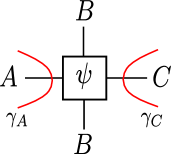
a)          b)    

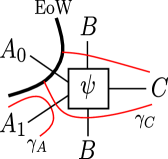
Figure 12: Minimal surfaces. a) Before a projective measurement. b) After a projective measurement denoted by EoW, when $n_{C}>n_{B}$.

Leveraging this interpretation of projective measurements as EoW brane-like objects, entanglement cross section can be identified as

$$E^{W}(A:B)=\min\left({\begin{array}[]{c}\vbox{\vskip 6.0pt\hbox{\hskip 4.0pt\includegraphics[scale={2.0}]{fig_Haar_cross_A}}}\end{array}}\ {\begin{array}[]{c}\vbox{\vskip 6.0pt\hbox{\hskip 4.0pt\includegraphics[scale={2.0}]{fig_Haar_cross_B}}}\end{array}}\right)\ \approx\min(n_{A},n_{B})$$ (88)

and $J^{W}(A|C)$ is given by

$$J^{W}(A|C)\approx S_{A}-E^{W}(A:B)=\max(0,n_{A}-n_{B}).$$ (89)

Our central proposal concerning LOCC entanglement distillation is $E_{D}^{[\text{G-LOCC}]}(A:C)=\max(J^{W}(A|C),J^{W}(C|A))$. Hence, for Haar random states, our proposal reads

$$\boxed{\ E_{D}^{[\text{G-LOCC}]}(A:C)\approx\text{hash}(A:C)\ }$$ (90)

at the leading order where $\text{hash}(A:C)$ coincides with maximum of $J^{W}(A|C)$ and $J^{W}(C|A)$. Indeed, if we consider “G-LOCCs” for Haar random states as LOCCs involving projective measurements in a random basis on $A$ and $C$ with only one round of CCs, the above distillation protocol is optimal since post-measurement states can be treated as Haar random states.

To the best of our knowledge, whether this result applies to generic LOCCs or not remains open. The main difficulty behind this generalization is that there may exist some special (fine-tuned) measurement basis whose post-measurement states have entanglement properties very distinct from those of Haar random states. For 1WAY LOCC protocols, a previous work [43] proved that the values of entanglement entropies in a post-measurement state match with those in a Haar random state. Relying on this result and focusing on one-shot settings, one can show

$$\boxed{\ E_{D}^{[\text{1WAY LOCC}]}(A:C)\approx\text{hash}(A:C)\ }$$ (91)

for Haar random states as further discussed in Section 6.

3 LO entanglement distillation in holography

In this section, we discuss LO-distillable entanglement $E_{D}^{[\text{LO}]}$ in holography. Our central proposal is that, if minimal surfaces $\gamma_{A}$ and $\gamma_{C}$ are separated in the bulk, $E_{D}^{[\text{LO}]}(A:C)\approx 0$ at the leading order in $1/G_{N}$. We have already argued that Haar random states satisfy this property. Here, we will further support this proposal by interpreting entanglement wedge reconstruction as an LO entanglement distillation problem. We will also present an argument for a random tensor network model of holography based on the performance of the Petz map.

3.1 Reconstruction and distillation

The conventional entanglement wedge reconstruction asserts that a bulk operator $\phi$ can be reconstructed on a boundary subsystem $A$ if $\phi$ is inside entanglement wedge $\mathcal{E}_{A}$ [60]. It will be useful to rephrase it as the entanglement distillation problem as suggested in [45]. Assume that bulk DOFs $Q$ are encoded into the boundary via an isometry $\Lambda:\mathcal{H}_{\text{bulk}}\rightarrow\mathcal{H}_{\text{bdy}}$ as $\Lambda(|j\rangle_{\text{bulk}})=|\psi_{j}\rangle_{\text{bdy}}$. We consider the case where bulk DOFs $Q$ are nearly maximally mixed, $\rho_{Q}\propto I_{Q}$. By using the Choi isomorphism, one can then construct a global pure state:

$$|\Psi\rangle\propto\sum_{j}|j\rangle_{\text{bulk}}\otimes|\psi_{j}\rangle_{\text{bdy}}$$ (92)

that includes both bulk and boundary DOFs. Note that the Choi state interpretation emerges naturally in tensor network toy models where the bulk open tensor legs and boundary tensor legs constitute the Choi state $|\Psi\rangle$ [27, 28].

That bulk DOFs $Q$ are encoded into boundary DOFs can be seen in that $Q$ are maximally entangled with boundary DOFs. Similarly, bulk DOFs $Q$ will be maximally entangled with boundary DOFs in $A$ when $Q$ can be reconstructed from the boundary subsystem $A$. Namely, by applying the Petzs map on the boundary subsystem $A$, one can LO-distill $S_{Q}$ (approximate) EPR pairs between $Q$ and $A$. Hence, entanglement wedge reconstruction can be interpreted as one-shot LO entanglement distillation, quantified by $E_{D}^{[\text{LO}]}(Q:A)$. It is worth emphasizing again that LO entanglement distillation can be performed by employing the standard (untwirled) Petz map instead of the improved (twirled) Petz map, due to the result by Barnum and Knill as discussed in the previous section. This is essentially due to that entanglement distillation characterizes the average reconstruction fidelity while the operator reconstruction can be affected by the worst case errors.

So far, we have argued that EPR pairs can be LO-distilled if $Q$ is contained inside $\mathcal{E}_{A}$. Our central hypothesis is that this statement can be promoted to an if and only if statement.

Hypothesis 3.

If bulk DOFs $Q$ are inside entanglement wedge $\mathcal{E}_{A}$ of a boundary subsystem $A$, one can distill $S_{Q}$ EPR pairs between $Q$ and $A$ by applying the Petz recovery map on $A$. If bulk DOFs $Q$ are outside $\mathcal{E}_{A}$, EPR pairs cannot be locally distilled between $Q$ and $A$ at the leading order in $1/G_{N}$.

Here, by $Q$ being outside $\mathcal{E}_{A}$, we mean that no part of $Q$ is inside $\mathcal{E}_{A}$ or Planck-scale close to the minimal surface $\gamma_{A}$.

At first sight, this claim (the only if part) might not appear very non-trivial. Indeed, when bulk DOFs carry subleading entropies only, this claim can be easily derived. Recall that, at the leading order, entanglement wedge $\mathcal{E}_{A}$ is given by the bulk subregion enclosed by the boundary subsystem $A$ and its minimal area surface $\gamma_{A}$. This implies that minimal surfaces of $A$ and $A^{c}$ must match, $\gamma_{A}=\gamma_{A^{c}}$, and thus, entanglement wedges $\mathcal{E}_{A}$ and $\mathcal{E}_{A^{c}}$ cover the whole bulk (except minimal surfaces $\gamma_{A}=\gamma_{A^{c}}$). This suggests that the bulk DOFs $Q$ are contained in $\mathcal{E}_{A}$ or $\mathcal{E}_{A^{c}}$, unless $Q$ sits exactly on $\gamma_{A}$. Recalling the monogamy of entanglement relation, $Q$ cannot be simultaneously entangled with $A$ and $A^{c}$. This suggests that, if $Q$ is outside $\mathcal{E}_{A}$, no EPR pairs can be distilled between $Q$ and $A$.

3.2 Shadow of entanglement wedge

We now turn to the cases where bulk DOFs, to be reconstructed on the boundary, carry leading order entropy. We begin by ignoring the effect of backreaction on the geometry. Recall that, for static cases, the entanglement wedge is computed by minimizing the generalized entropy

$$S_{A}=\min_{\gamma_{A}}\frac{\text{Area}(\gamma_{A})}{4G_{N}}+S_{\text{bulk}}$$ (93)

where $S_{\text{bulk}}$ is a bulk entropy on a subregion surrounded by $\gamma_{A}$. The crucial difference is that the minimal entropy surface $\gamma_{A}$ is not necessarily given by the minimal area surface $\gamma_{A}^{\text{area}}$ at the leading order due to that $S_{\text{bulk}}=O(1/G_{N})$. This creates an interesting situation where minimal entropy surfaces of $A$ and its complement $A^{c}$ may not match, $\gamma_{A}\not=\gamma_{A^{c}}$, and there can be a bulk subregion which is not contained in either $\mathcal{E}_{A}$ or $\mathcal{E}_{A^{c}}$. We shall call such a bulk subregion shadow of entanglement wedges with respect to the bipartition $A,A^{c}$. See Fig. 13(a)for an example of shadow of entanglement wedges.

Note that shadow of entanglement wedge is different from entanglement shadow which corresponds to a bulk subregion where no minimal surface $\gamma_{A}^{\text{area}}$, for any choice of $A$, can go through [63]. Here we consider a bulk subregion that cannot be covered by $\mathcal{E}_{A},\mathcal{E}_{A^{c}}$ for a fixed bipartition $A,A^{c}$.

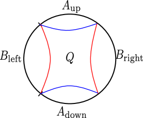
a)     b)     c)    

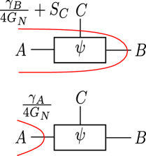
Figure 13: a) This setup was originally considered in [61]. The boundary is divided into four segments of roughly equal sizes and organized into $A$ and $B$. When $S_{Q}=O(1/G_{N})$, $Q$ is outside $\mathcal{E}_{A}$ and $\mathcal{E}_{B}$. One may replace $Q$ with a small (sub-AdS size) black hole or a conical singularity in order to explicitly account for backreaction. b) A Haar random state as a bulk-to-boundary map. c) Two candidate entropies for computing $S_{A}$. The first candidate is given by the minimal area $\gamma_{A}$ while the second candidate entropy is given by the minimal area $\gamma_{B}$ plus the bulk contribution $S_{C}$.

The crux of the aforementioned hypothesis can be then rephrased as follows.

Hypothesis 4.

If bulk DOFs $Q$ are in shadow of entanglement wedge (i.e. outside $\mathcal{E}_{A}$ and $\mathcal{E}_{A^{c}}$), we have

$$E_{D}^{[\text{LO}]}(Q:A),E_{D}^{[\text{LO}]}(Q:A^{c})\approx 0$$ (94)

at the leading order.

In the next subsection, we will prove this hypothesis for random tensor networks in some particular regimes.

When $Q$ is in the shadow of $\mathcal{E}_{A}$ and $\mathcal{E}_{A^{c}}$, we often have large mutual information with $I(A:Q),I(A^{c}:Q)=O(1/G_{N})$. Entanglement wedge reconstruction and our hypothesis, as stated above, suggest that, despite $O(1/G_{N})$ mutual information, no EPR pairs can be LO-distilled at the leading order.

It is worth recalling that we have already seen a similar phenomenon in Haar random states. Namely, as in Fig. 13(b), by interpreting $C$ as bulk DOFs, we find that $C$ is in the shadow of entanglement wedge as it is outside $\mathcal{E}_{A}$ and $\mathcal{E}_{B}$.

In the discussions above, we have ignored the effect of backreaction resulting from $O(1/G_{N})$ bulk DOFs. To properly account for backreaction, one may consider distillation problems in a backreacted geometry. For instance, in the setup of Fig. 13(a), we may collapse bulk DOFs $Q$ into a massive object which may be treated as a conical singularity at the center. We may also consider a small (sub AdS scale) black hole and associate bulk DOFs to the black hole entropy. As long as bulk DOFs $Q$ are located near the center of the bulk and away from minimal surfaces of $A$ and $B$, the core of our argument will remain valid.

Finally, let us discuss the implication of the aforementioned hypothesis concerning entanglement distillation and entanglement wedge reconstruction. Let us focus on the setup in AdS₃ as shown in Fig. 14. By coarse-graining boundary subsystem $C$ in the radial direction, one can associate DOFs in $C$ to those on the minimal surface $\gamma_{C}$ with an approximate isometry $\gamma_{C}\rightarrow C$. Such a map can be explicitly constructed in tensor network models of holography. Furthermore, coarse-grained DOFs on $\gamma_{C}$ are nearly maximally entangled with $AB$. Hence, we can interpret $\gamma_{C}$ as bulk DOFs which are to be reconstructed on boundary DOFs $AB$. We then observe that $\gamma_{C}$ is outside $\mathcal{E}_{A}$ as the minimal surface $\gamma_{A}$ is separated from $\gamma_{C}$ in the bulk. This suggests that $E_{D}^{[\text{LO}]}(A:C)\approx 0$ at the leading order.

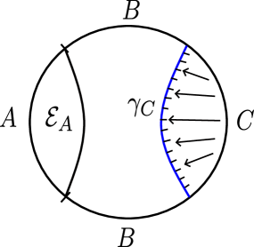
Figure 14: An example in the pure AdS₃ with $E_{D}^{[\text{LO}]}(A:C)\approx 0$ at the leading order. Here, $\gamma_{C}$ is interpreted as bulk DOFs which are to be reconstructed from $AB$. LO entanglement distillation is not possible as $\gamma_{C}$ is not inside $\mathcal{E}_{A}$.

3.3 Bound from the Petz map

Finally, we present an upper bound on $E_{D}^{[\text{LO}]}(A:C)$ by studying the decoding performance of the Petz map for random tensor network states. The argument parallels the one from Section 2. Applying the Petz map generates the double-copy state of the following form:

$${\begin{array}[]{c}\vbox{\vskip 6.0pt\hbox{\hskip 4.0pt\includegraphics[scale={2.0}]{fig_TN_glue}}}\end{array}}$$ (96)

where two copies $|\psi_{ABC}\rangle$ and $|\psi_{ABC}^{*}\rangle$ are glued at the minimal surface $\gamma_{C}$.

Let us evaluate the mutual information $I(A:A^{\prime})$. We find

$$S_{A}\approx{\begin{array}[]{c}\vbox{\vskip 6.0pt\hbox{\hskip 4.0pt\includegraphics[scale={2.0}]{fig_TN_glue_RT_A_geo_left}}}\end{array}},\qquad S_{A^{\prime}}\approx{\begin{array}[]{c}\vbox{\vskip 6.0pt\hbox{\hskip 4.0pt\includegraphics[scale={2.0}]{fig_TN_glue_RT_A_geo_right}}}\end{array}}$$ (99)

whereas

$$S_{AA^{\prime}}\approx\min\quantity[{\begin{array}[]{c}\vbox{\vskip 5.40001pt\hbox{\hskip 3.6pt\includegraphics[scale={1.8}]{fig_TN_glue_RT_A_geo}}}\end{array}},\ {\begin{array}[]{c}\vbox{\vskip 5.40001pt\hbox{\hskip 3.6pt\includegraphics[scale={1.8}]{fig_TN_glue_RT_B_geo}}}\end{array}}]$$ (102)

as shown in Appendix D. Recalling the definition of entanglement wedge cross section $E^{W}(A:B)$, we have

$$S_{AA^{\prime}}\approx 2E^{W}(A:B)$$ (103)

and thus

$$\boxed{\frac{1}{2}I(A:A^{\prime})\approx J^{W}(A|C)\equiv S_{A}-E^{W}(A:B).\ }$$ (104)

Hence, $E_{D}^{[\text{LO}]}(A:C)\lesssim J^{W}(A|C)$. Repeating the same argument by exchanging $A$ and $C$, we find

$$\boxed{\ E_{D}^{[\text{LO}]}(A:C)\lesssim\min(J^{W}(A|C),J^{W}(C|A)).\ }$$ (105)

While this bound is weaker than what we expect (namely $E_{D}^{[\text{LO}]}(A:C)\approx 0$), this proves the existence of holographic $\rho_{AC}$ satisfying

$$E_{D}^{[\text{LO}]}(A:C)\approx 0,\qquad I(A:C)\sim O(1/G_{N}),$$ (106)

where $1/G_{N}$ should be interpreted as the entropy unit carried in each tensor leg. In the next section, we will show

$$E_{D}^{[\text{LOCC}]}(A:C)\gtrsim\max(J^{W}(A|C),J^{W}(C|A))$$ (107)

by presenting an explicit distillation protocol. Hence, there exists a regime in holography where

$$E_{D}^{[\text{LO}]}(A:C)<E_{D}^{[\text{LOCC}]}(A:C)$$ (108)

with an $O(1/G_{N})$ gap between LO and LOCC distillable entanglement at the leading order.

Finally, it is worth noting that this bound on $E_{D}^{[\text{LO}]}$, based on the performance of the Petz map, applies to the entanglement wedge reconstruction problem. In particular, let us revisit the setup as in Fig. 13(a) where the boundary is divided into $A$ and $B$, and bulk DOFs $Q$ are sitting at the center of the AdS₃ and are located far from $\gamma_{A},\gamma_{B}$. When the sizes of $A$ and $B$ are comparable, we expect $J^{W}(A|Q),J^{W}(B|Q)\approx 0$. Hence, we have $E_{D}^{[\text{LO}]}(Q:A),E_{D}^{[\text{LO}]}(Q:B)\approx 0$, and thus Hypothesis 4, concerning a shadow of entanglement wedge, can be rigorously proven in such regimes.

4 LOCC entanglement distillation in holography

In this section, we present an LOCC protocol that distills $J^{W}(A|C)\equiv S_{A}-E^{W}(A:B)$ EPR pairs. We then show that this protocol is optimal under G-LOCCs.

4.1 Distillation protocol

For simplicity of presentation, we focus on the pure AdS₃ setup from Fig. 1. Furthermore, we work on a regime with

$$J^{W}(C|A)\equiv S_{C}-E^{W}(B:C)>0.$$ (109)

This condition can be schematically depicted as

$${\begin{array}[]{c}\vbox{\vskip 6.0pt\hbox{\hskip 4.0pt\includegraphics[scale={2.0}]{fig_SC}}}\end{array}}\ >\ {\begin{array}[]{c}\vbox{\vskip 6.0pt\hbox{\hskip 4.0pt\includegraphics[scale={2.0}]{fig_EWBC}}}\end{array}}.$$ (112)

The protocol performs projective measurements on DOFs associated with a portion of the minimal surface $\gamma_{A}$. Let us split $\gamma_{A}$ into two parts $\gamma_{A}=\gamma_{A_{0}}\cup\gamma_{A_{1}}$ as depicted in Fig. 15.

1. Perform projective measurements on $\gamma_{A_{0}}$ in disentangled basis and leave the remaining part $\gamma_{A_{1}}$ untouched.

2. Send the measurement outcome from $A$ to $C$.

3. Run the Petz recovery map on $C$ to distill $\frac{1}{4G_{N}}\text{Area}(\gamma_{A_{1}})$ copies of EPR pairs.

Here we take $\gamma_{A_{0}}$ large enough so that the entanglement wedge cross section $\Sigma_{B:C}$ anchors on $\gamma_{A_{0}}$ as shown in Fig. 15. Note that the post-measurement state has a semiclassical dual geometry with EoW brane-like objects [24]. Namely, regardless of the measurement outcomes, we have the same geometry due to that measurements were performed in a random basis. We also choose the area (length) of $\gamma_{A_{1}}$ so that the remaining portion $\gamma_{A_{1}}$ carries $\frac{1}{4G_{N}}\text{Area}(\gamma_{A_{1}})\approx J^{W}(C|A)$ entropy. This is possible since, otherwise, $\gamma_{C}$ would not be the minimal surface of $C$.

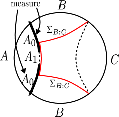
Figure 15: An LOCC entanglement distillation protocol in holography. The protocol places EoW brane-like objects on a portion of $\gamma_{A}$.

The third step distills EPR pairs since, in the post-measurement state, the minimal surface $\gamma_{C}$ changes its profile and overlaps with $\gamma_{A_{1}}$ due to placing the EoW brane-like objects via projective measurements. Namely, two candidate surfaces for $C$ satisfy

$${\begin{array}[]{c}\vbox{\vskip 6.0pt\hbox{\hskip 4.0pt\includegraphics[scale={2.0}]{fig_remaining}}}\end{array}}\ \approx\ {\begin{array}[]{c}\vbox{\vskip 6.0pt\hbox{\hskip 4.0pt\includegraphics[scale={2.0}]{fig_SC}}}\end{array}}$$ (115)

since we choose $\frac{1}{4G_{N}}\text{Area}(\gamma_{A_{1}})\approx J^{W}(C|A)$. Note that there is no contribution from a portion of the curve overlapping with the thick black curves, denoting the EoW brane-like objects. By exchanging $A$ and $C$, one obtains a protocol distilling $J^{W}(A|C)$ EPR pairs.

It is worth noting that this protocol beats the hashing bound. Namely, by the definition of $E^{W}$, we have

$$S_{AC}={\begin{array}[]{c}\vbox{\vskip 6.0pt\hbox{\hskip 4.0pt\includegraphics[scale={2.0}]{fig_SAC}}}\end{array}}\ \geq E^{W}(B:C)={\begin{array}[]{c}\vbox{\vskip 6.0pt\hbox{\hskip 4.0pt\includegraphics[scale={2.0}]{fig_EWBC}}}\end{array}}$$ (118)

which implies $S_{C}-S_{AC}\leq S_{C}-E^{W}(B:C)$. Hence we have

$$\boxed{\ \text{hash}(A:C)\leq J^{W}(A:C)\ }$$ (119)

beating the hashing bound.

4.2 Locally accessible information

Recall that gravitational locally accessible information $J^{G}(A|C)$ (Eq. (33)) corresponds to the maximal possible entropy drop $\Delta S_{A}=S_{A}^{\text{before}}-S_{A}^{\text{after}}$, on average, due to holographic measurements on $C$. It is then immediate to see

$$\boxed{\ J^{G}(A|C)\approx J^{W}(A|C)\ }$$ (120)

at the leading order, as the EoW brane placed on $\gamma_{C}$ achieves $\Delta S_{A}\approx J^{W}(A|C)$:

$$S_{A}^{\text{before}}=\frac{1}{4G_{N}}{\begin{array}[]{c}\vbox{\vskip 6.0pt\hbox{\hskip 4.0pt\includegraphics[scale={2.0}]{fig_SA}}}\end{array}}\,,\qquad S_{A}^{\text{after}}=\frac{1}{4G_{N}}{\begin{array}[]{c}\vbox{\vskip 6.0pt\hbox{\hskip 4.0pt\includegraphics[scale={2.0}]{fig_EWAB}}}\end{array}}.$$ (123)

Here, performing projective measurements along $\gamma_{C}$ in a local random basis always creates the same geometry and thus the same $S_{A}^{\text{after}}$ at the leading order. Finally, we can observe that placing EoW brane-like objects on other locations would make $S_{A}^{\text{after}}$ larger. An explicit calculation of $J^{W}(A|C)$ in the pure AdS₃ is presented in Appendix A.

4.3 1WAY Optimality of the protocol

Let us begin by presenting a definition of G-LOCCs. Given a holographic density matrix $\rho_{AC}$ with semiclassical dual, a G-LOCC performs the following three-step operations (Fig. 16).

1. Perform holographic measurements on $A$ and $C$ in a local random basis, which place EoW brane-like objects on some portions in $\mathcal{E}_{A}$ and $\mathcal{E}_{C}$.

2. Send measurement outcomes to other parties.

3. Perform local operations, acting individually on $A$ and $C$, to distill EPR pairs between $A$ and $C$.

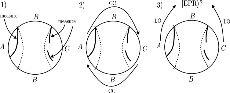
Figure 16: G-LOCC. It performs 1) holographic measurements, 2) one round of CCs, and 3) LOs.

One important limitation of G-LOCCs should be emphasized. In conventional LOCCs, one party may optimize the measurement basis after learning the measurement outcome of the other party. On the contrary, in G-LOCCs, holographic measurements on $A$ and $C$ are performed in a random basis regardless of measurement outcomes in other parties by allowing each party to send measurement outcomes only after completing all the measurements. This restriction, disallowing multiple rounds of exchanges of classical communications, appears naturally in various phenomena in holography. Namely, traversable wormholes and holographic scattering, which will be further discussed in the next section, allow only one round of classical communication. See Fig. 17 for a comparison among 1WAY, 2WAY with one round of CC (including G-LOCCs), and 2WAY entanglement distillation protocols.

Figure 17: 1WAY v.s. 2WAY with one round of CC v.s. 2WAY. In a 1WAY protocol, only one side can perform a measurement and send the outcome to the other. The receiver can only perform an LO depending on the received outcomes. In a 2WAY protocol with one round of CC, each side can independently perform a measurement and send measurement outcomes to each other. After that, they can only perform an LO depending on the received outcomes. G-LOCC protocols belong to this class of protocols. In 2WAY protocols, both sides can feedforward the measurement outcomes and they can adjust the next measurement operator $\mathcal{M}$ depending on the outcomes.

Conventionally, an LOCC between $A$ and $C$ allows sending CCs from both parties, and thus can use 2WAY CCs. In contrast, our LOCC protocol is 1WAY as it sends CCs only from $A$ to $C$. We claim that the aforementioned protocol is optimal under 1WAY G-LOCCs, namely

$$\boxed{\ E_{D}^{[\text{1WAY G-LOCC}](A\rightarrow C)}(A:C)\approx J^{W}(C|A).\ }$$ (124)

To prove this statement, let us suppose that there exists a 1WAY G-LOCC protocol that distills more than $J^{W}(C|A)$ EPR pairs by measuring $A_{0}\subset A$. Let $\sigma_{AC}^{j_{A}}$ be a post-measurement state with $j_{A}$ denoting the measurement outcome. In the previous section, we derived an upper bound (Eq. (105)) on $E_{D}^{[\text{LO}]}(A:C)$ by using the performance of the Petz map. Noting that $\sigma_{AC}^{j_{A}}$ is also a holographic state with semiclassical dual, we can apply this bound to $\sigma_{AC}^{j_{A}}$ and obtain

$$E_{D}^{[\text{LO}]}(A:C)(\sigma_{AC}^{j_{A}})\lesssim J^{W}(C|A)(\sigma_{AC}^{j_{A}}).$$ (125)

Here, we claim the following inequality, which will be proven shortly:

$$\boxed{\ J^{W}(C|A)(\sigma_{AC}^{j_{A}})\lesssim J^{W}(C|A)(\rho_{AC})\ }$$ (126)

which essentially says that holographic measurements on $A$ will never make $J^{W}(C|A)$ larger. This inequality then suggests $E_{D}^{[\text{LO}]}(A:C)(\sigma_{AC}^{j_{A}})\lesssim J^{W}(C|A)(\rho_{AC})$, which leads to a contradiction. As such, Eq. (124) follows from Eq. (126).

The remaining task is to prove the inequality in Eq. (126). Recall that

$$\begin{split}J^{G}(C|A)(\rho_{AC})\approx J^{W}(C|A)(\rho_{AC})&\equiv S_{C}(\rho_{C})-E^{W}(B:C)(\rho_{BC})\\ J^{G}(C|A)(\sigma_{AC}^{j_{A}})\approx J^{W}(A|C)(\rho_{AC})&\equiv S_{C}(\sigma_{C}^{j_{A}})-E^{W}(B:C)(\sigma_{BC}^{j_{A}}).\end{split}$$ (127)

One can show

$$S_{C}(\sigma_{C}^{j_{A}})\leq S_{C}(\rho_{C})$$ (128)

by writing the average entropy drop due to measurements on $A_{0}$ as

$$\Delta S_{C}=S_{C}(\rho_{C})-\sum_{j_{A}}p_{j_{A}}S_{C}(\sigma_{C}^{j_{A}})=\sum_{j}p_{j_{A}}S(\sigma_{C}^{j_{A}}\|\rho_{C})\geq 0,$$ (129)

using the positivity of the relative entropy, and observing that $S_{C}(\sigma_{C}^{j_{A}})$ does not depend on $j_{A}$ at the leading order (since $\sigma_{C}^{j_{A}}$ almost surely have the same geometry). One can also show

$$E^{W}(B:C)(\sigma_{BC}^{j_{A}})\geq E^{W}(B:C)(\rho_{BC})$$ (130)

by observing that the minimal surface $\gamma_{A}$ for $\sigma_{ABC}^{j_{A}}$ does not extend beyond the minimal surface $\gamma_{A}$ for $\rho_{ABC}$ since holographic measurements on $A_{0}$ can place EoW brane-like objects only inside $\mathcal{E}_{A}$ for $\rho_{ABC}$. Hence, we obtain Eq. (126).

Finally, exchanging $A$ and $C$ and repeating the same argument, we arrive at

$$\boxed{\ E_{D}^{[\text{1WAY G-LOCC}]}(A:C)\approx J^{W}(A:C).\ }$$ (131)

4.4 2WAY Optimality of the protocol

We have shown that the aforementioned protocol is optimal under 1WAY G-LOCC. We now show that it is optimal under (2WAY) G-LOCC.

Assume that holographic measurements are performed on $A_{0}$ and $C_{0}$. Let $\sigma_{AC}^{j_{C}}$ be the post-measurement state after measuring $C_{0}$ with an outcome $j_{C}$, but before measuring $A_{0}$. Schematically, we have

$$\rho_{AC}\underset{\text{measure $C$}}{\longrightarrow}\sigma_{AC}^{j_{C}}\underset{\text{measure $A$}}{\longrightarrow}\sigma_{AC}^{i_{A}j_{C}}.$$ (132)

Note that $\sigma_{AC}^{j_{C}}$ are holographic states with a semiclassical dual. Namely, they have the same geometry regardless of the measurement outcome $j_{C}$. Observing that the 2WAY G-LOCC protocol can be interpreted as 1WAY G-LOCC protocol applied for $\sigma_{AC}^{j_{C}}$, the distillable entanglement for $\rho_{AC}$ under G-LOCCs is upper bounded by

$$\lesssim\max\big{(}J^{W}(A|C)(\sigma_{AC}^{j_{C}}),J^{W}(C|A)(\sigma_{AC}^{j_{C}})\big{)}.$$ (133)

In fact, this is potentially a loose upper bound. Recall that only one round of CCs is allowed in G-LOCCs. This implies that holographic measurements on $A$ can place EoW brane-like objects only inside $\mathcal{E}_{A}$ of the original pre-measurement state $\rho_{AC}$ since $A$ needs to decide on the measurement basis before receiving measurement outcomes from $C$. Hence, the distillable entanglement can be upper bounded by

$$\lesssim\max\big{(}J^{W}(A|C)(\sigma_{AC}^{j_{C}}),\widetilde{J^{W}}(C|A)(\sigma_{AC}^{j_{C}})\big{)}$$ (134)

where $\widetilde{J^{W}}(C|A)(\sigma_{AC}^{j_{C}})$ represents gravitational locally accessible information when holographic measurements on $A$ are restricted to be inside $\mathcal{E}_{A}$ of the original state $\rho_{AC}$. Note that we have $\widetilde{J^{W}}(C|A)(\sigma_{AC}^{j_{C}})\leq J^{W}(C|A)(\sigma_{AC}^{j_{C}})$ by definition.

Our goal is to show that the above upper bound can be further upper bounded by

$$\lesssim J^{W}(A:C)(\rho_{AC})\equiv\max\big{(}J^{W}(A|C)(\rho_{AC}),J^{W}(C|A)(\rho_{AC})\big{)}.$$ (135)

This will prove that the aforementioned G-LOCC protocol is optimal under (2WAY) G-LOCCs at the leading order. From Eq. (126), we already know that

$$J^{W}(A|C)(\sigma_{AC}^{j_{C}})\lesssim J^{W}(A|C)(\rho_{AC}).$$ (136)

(Here, we exchanged $A$ and $C$ in Eq. (126)). Hence, it suffices to show the following inequality:

$$\boxed{\ \widetilde{J^{W}}(C|A)(\sigma_{AC}^{j_{C}})\lesssim J^{W}(C|A)(\rho_{AC}).\ }$$ (137)

Notice that this is different from Eq. (126). Namely, this concerns $\sigma_{AC}^{j_{C}}$ after measurements on $C$ whereas Eq. (126) concerns $\sigma_{AC}^{j_{A}}$ after measurements on $A$. Here, we emphasize again that, in evaluating $\widetilde{J^{W}}(C|A)(\sigma_{AC}^{j_{C}})$, holographic measurements inside $\mathcal{E}_{A}$ of $\rho_{AC}$ are considered.

Below, we show Eq. (137) by focusing on the setup depicted in Fig. 1 in the pure AdS₃. We expect that our arguments apply to generic setups in holography. Here, we begin with the cases where measured DOFs $A_{0}$ and $C_{0}$ are portions of $\gamma_{A}$ and $\gamma_{C}$ respectively (i.e. projective measurements are performed on boundaries of $\mathcal{E}_{A}$ and $\mathcal{E}_{C}$). There will be three types of minimal surfaces for $C$ which play important roles in our argument:

$$\begin{split}&\gamma_{C}^{\text{before}}\ \ \ \ \text{: defined for the original state $\rho_{AC}$}\\ &\gamma_{C}^{\text{after-$C$}}\ \ \ \text{: defined for the state $\rho_{AC}^{j_{C}}$ after measuring $C$}\\ &\gamma_{C}^{\text{after-$AC$}}\ \text{: defined for the state $\rho_{AC}^{i_{A}j_{C}}$ after measuring $A$ and $C$}\end{split}$$ (138)

and we also denote

$$\gamma_{A}^{\text{before}}\ \ \ \ \text{: defined for the original state $\rho_{AC}$.}\qquad\qquad\qquad\qquad$$ (139)

Since holographic measurements on $C$ are performed on the minimal surface $\gamma_{C}^{\text{before}}$, $\gamma_{C}^{\text{before}}$ and $\gamma_{C}^{\text{after-$C$}}$ will have the same profile. Note that, however, the entropy corresponding to $\gamma_{C}^{\text{after-$C$}}$ is smaller than $S_{C}(\rho_{AC})$, the entropy corresponding to $\gamma_{C}^{\text{before}}$ since the area of the surfaces along the EoW brane-like objects does not contribute to the RT formula.

Let us schematically depict $\gamma_{C}^{\text{after-$C$}}$ as follows

$$S_{C}(\rho_{AC}^{j_{C}})=\frac{1}{4G_{N}}{\begin{array}[]{c}\vbox{\vskip 6.0pt\hbox{\hskip 4.0pt\includegraphics[scale={2.0}]{fig_2WAY_C}}}\end{array}}$$ (141)

where black thick lines represent measured portions on $C$. We now evaluate the entropy drop due to holographic measurements on $A$. Without loss of generality, we may assume that a non-zero entropy drop can be achieved. In order to have nonzero entropy drop, $\gamma_{C}^{\text{after-$AC$}}$ must differ from $\gamma_{C}^{\text{after-$C$}}$. Since the entropy drop occurs due to placing EoW brane-like objects on $\gamma_{A}^{\text{before}}$, $\gamma_{C}^{\text{after-$AC$}}$ must touch $\gamma_{A}^{\text{before}}$ at least once. (If this is not the case, $\gamma_{C}^{\text{after-$AC$}}$ would have been chosen as a minimal surface of $C$ for $\sigma_{AC}^{j_{C}}$). Hence, $\gamma_{C}^{\text{after-$AC$}}$ must exit $\gamma_{C}^{\text{before}}$, touch $\gamma_{A}^{\text{before}}$, and then eventually return to $\gamma_{C}^{\text{before}}$. This is schematically depicted below

$$S_{C}(\rho_{AC}^{i_{A}j_{C}})=\frac{1}{4G_{N}}{\begin{array}[]{c}\vbox{\vskip 6.0pt\hbox{\hskip 4.0pt\includegraphics[scale={2.0}]{fig_2WAY_AC}}}\end{array}}\ .$$ (143)

In principle, $\gamma_{C}^{\text{after-$AC$}}$ may go back and forth multiple times between $\gamma_{C}^{\text{before}}$ and $\gamma_{A}^{\text{before}}$. In the above figure, for simplicity of discussion and drawing, we considered the case where $\gamma_{C}^{\text{after-$AC$}}$ go back and forth only one time. We would like to note that our argument below easily generalizes to the cases where $\gamma_{C}^{\text{after-$AC$}}$ consist of multiple round trips.

The entropy drop due to this holographic measurement on $A$ is given by

$$\Delta S_{C}=\frac{1}{4G_{N}}\quantity({\begin{array}[]{c}\vbox{\vskip 6.0pt\hbox{\hskip 4.0pt\includegraphics[scale={2.0}]{fig_2WAY_C}}}\end{array}}\ -\ {\begin{array}[]{c}\vbox{\vskip 6.0pt\hbox{\hskip 4.0pt\includegraphics[scale={2.0}]{fig_2WAY_AC}}}\end{array}})$$ (146)

where EoW brane-like objects are placed on $\gamma_{A}^{\text{before}}$. Focusing on the portions where $\gamma_{C}^{\text{after-$C$}}$ and $\gamma_{C}^{\text{after-$AC$}}$ do not match, we have

$$\begin{split}\Delta S_{C}&=\frac{1}{4G_{N}}\quantity({\begin{array}[]{c}\vbox{\vskip 6.0pt\hbox{\hskip 4.0pt\includegraphics[scale={2.0}]{fig_2WAY_C_portion}}}\end{array}}\ -\ {\begin{array}[]{c}\vbox{\vskip 6.0pt\hbox{\hskip 4.0pt\includegraphics[scale={2.0}]{fig_2WAY_AC_portion}}}\end{array}}\ )\\ &\lesssim\frac{1}{4G_{N}}\quantity({\begin{array}[]{c}\vbox{\vskip 6.0pt\hbox{\hskip 4.0pt\includegraphics[scale={2.0}]{fig_2WAY_C_portion2}}}\end{array}}\ -\ {\begin{array}[]{c}\vbox{\vskip 6.0pt\hbox{\hskip 4.0pt\includegraphics[scale={2.0}]{fig_2WAY_AC_portion2}}}\end{array}}\ )\end{split}$$ (147)

where the inequality results from removing the portion of the curve sitting on $\gamma_{A}^{\text{before}}$ in the second diagram. By restoring the portion where $\gamma_{C}^{\text{after-$A$}}$ and $\gamma_{C}^{\text{after-$AC$}}$ overlap, and removing EoW brane-like objects in the overlapping portion, the above quantity can be further upper bounded by

$$\begin{split}&=\frac{1}{4G_{N}}\quantity({\begin{array}[]{c}\vbox{\vskip 6.0pt\hbox{\hskip 4.0pt\includegraphics[scale={2.0}]{fig_2WAY_C_portion3}}}\end{array}}\ -\ {\begin{array}[]{c}\vbox{\vskip 6.0pt\hbox{\hskip 4.0pt\includegraphics[scale={2.0}]{fig_2WAY_AC_portion3}}}\end{array}}\ )\\ &\lesssim\frac{1}{4G_{N}}\quantity({\begin{array}[]{c}\vbox{\vskip 6.0pt\hbox{\hskip 4.0pt\includegraphics[scale={2.0}]{fig_2WAY_C_portion3}}}\end{array}}\ -\ {\begin{array}[]{c}\vbox{\vskip 6.0pt\hbox{\hskip 4.0pt\includegraphics[scale={2.0}]{fig_2WAY_AC_portion4}}}\end{array}}\ )\\ &\lesssim J^{W}(C|A)(\rho_{AC})\end{split}$$ (148)

where the inequality in the second line follows from the minimality of the cross section $\Sigma_{B:C}$. Hence, we arrive at Eq. (137).

Next, we consider the cases where $C_{0}$ does not necessarily sit on $\gamma_{C}^{\text{before}}$ while $A_{0}$ sits on $\gamma_{A}^{\text{before}}$. Let us schematically depict $\gamma_{C}^{\text{after-$C$}}$ and $\gamma_{C}^{\text{after-$AC$}}$ as follows

$$S_{C}(\rho_{AC}^{j_{C}})=\frac{1}{4G_{N}}{\begin{array}[]{c}\vbox{\vskip 6.0pt\hbox{\hskip 4.0pt\includegraphics[scale={2.0}]{fig_2WAY_C_portion_in}}}\end{array}},\qquad S_{C}(\rho_{AC}^{i_{A}j_{C}})=\frac{1}{4G_{N}}{\begin{array}[]{c}\vbox{\vskip 6.0pt\hbox{\hskip 4.0pt\includegraphics[scale={2.0}]{fig_2WAY_AC_portion_in}}}\end{array}}$$ (151)

where $\gamma_{C}^{\text{after-$AC$}}$ must exists $\gamma_{C}^{\text{after-$C$}}$ and touch $\gamma_{A}^{\text{before}}$ in order to have nonzero entropy drop. Repeating a similar argument, we obtain

$$\Delta S_{C}\lesssim\frac{1}{4G_{N}}\quantity({\begin{array}[]{c}\vbox{\vskip 6.0pt\hbox{\hskip 4.0pt\includegraphics[scale={2.0}]{fig_2WAY_C_portion2_in}}}\end{array}}\ -\ {\begin{array}[]{c}\vbox{\vskip 6.0pt\hbox{\hskip 4.0pt\includegraphics[scale={2.0}]{fig_2WAY_AC_portion2_in}}}\end{array}}\ )$$ (154)

Here, we claim

$${\begin{array}[]{c}\vbox{\vskip 6.0pt\hbox{\hskip 4.0pt\includegraphics[scale={2.0}]{fig_2WAY_total_in}}}\end{array}}\ \lesssim\ {\begin{array}[]{c}\vbox{\vskip 6.0pt\hbox{\hskip 4.0pt\includegraphics[scale={2.0}]{fig_2WAY_total}}}\end{array}}\ .$$ (157)

This claim follows from the minimality of $\gamma_{C}^{\text{after-$C$}}$. Let us label the curves as follows:

$${\begin{array}[]{c}\vbox{\vskip 6.0pt\hbox{\hskip 4.0pt\includegraphics[scale={2.0}]{fig_2WAY_length}}}\end{array}}.$$ (159)

Here, we have

$$d\lesssim b+c$$ (160)

since, otherwise $\gamma_{C}^{\text{after-$C$}}$ would have chosen the path going through $b$ and $c$, instead of $d$. With some inspection, we then notice that Eq. (160) implies Eq. (157). (Note LHS $=-a-c+d$ and RHS$=-a+b$.) Applying Eq. (157) to Eq. (154), we obtain

$$\Delta S_{C}\lesssim\frac{1}{4G_{N}}{\begin{array}[]{c}\vbox{\vskip 6.0pt\hbox{\hskip 4.0pt\includegraphics[scale={2.0}]{fig_2WAY_total}}}\end{array}}\lesssim J^{W}(C|A)(\rho_{AC})$$ (162)

where the last inequality follows from an argument similar to Eq. (148). Finally, we note that this argument easily generalizes to the cases where $A_{0}$ may not sit on $\gamma_{A}^{\text{before}}$. Hence, we have Eq. (137).

As such, we arrive at

$$\boxed{\ E_{D}^{[\text{G-LOCC}]}(A:C)\approx J^{W}(A:C).\ }$$ (163)

5 Subleading effects

In this section, we discuss possible subleading contributions to $E_{D}^{[\text{LO}]}$ and $E_{D}^{[\text{G-LOCC}]}$ by considering three potential physical mechanisms, namely a traversable wormhole, holographic scattering, and a Planck-scale effect.

Before starting, let us briefly discuss potential subleading contributions from bulk matter fields. We have assumed that bulk matter fields have subleading entropy to avoid backreaction to the geometry. Furthermore, as discussed in the introduction, we expect that the bulk matter field contribution to $E_{D}(A:C)$ will be negligibly small since correlations in matter fields between two entanglement wedges $\mathcal{E}_{A}$ and $\mathcal{E}_{C}$ decay exponentially with respect to their spatial separation. For this reason, our main focus in this section will be to explore subleading contributions to $E_{D}(A:C)$ which do not directly result from matter field entanglement.

5.1 Traversable wormhole

Traversable wormholes are phenomena where quantum information, thrown from one side of a two-sided AdS black hole of inverse temperature $\beta$ and Beckenstein-Hawking entropy $S_{\mathrm{BH}}$ at $t=0$, can reach the other side by introducing some special interaction that couples two sides:

$$U_{int}=\exp\quantity(-i\theta\sum_{j}O_{j}\otimes O_{j}^{*})$$ (164)

where $O_{j}$ are simple operators such as few-body Pauli or Majorana operators [64, 65, 66, 67, 68, 69]. This interaction, with specifically tuned phase $\theta(\tau)$, needs to be applied at $t_{L}\approx-t_{R}=\tau$ with $\tau>0$ satisfying $t_{th}\lesssim\tau\lesssim t_{scr}$ where $t_{th}$ and $t_{scr}$ represent thermal time $\sim\beta$ and scrambling time $\sim\beta\log S_{\mathrm{BH}}$ respectively.

At first glance, sending information through a wormhole might not strike surprising when two sides are directly coupled. What is truly surprising is that it utilizes pre-shared quantum entanglement between two sides in order to transmit information. This can be understood by reproducing the same phenomena with a protocol similar to quantum teleportation where the unitary coupling of Eq. (164) is replaced with LOCCs. Concretely, let us assume that $O_{j}$’s are mutually commuting single-body Pauli operators. One can send a signal through the wormhole by projectively measuring $O_{j}$ on the left and then applying the following on the right:

$$U_{R}=\exp\quantity(-i\theta\sum_{j}m_{j}O_{j}^{*})$$ (165)

where $m_{j}=\pm 1$ represents the measurement outcome of $O_{j}$. The quantum circuit diagram for this process is shown in Fig. 18(a). This process is described by LOCC as it involves measurements on one party and sends the outcomes through classical communications to the other party. That quantum information can be sent by an LOCC implies that the traversable wormhole utilizes pre-shared quantum entanglement between two parties.

To establish a connection with the entanglement distillation problem, we need a few more ingredients. We begin by pointing out that the traversable wormhole phenomena can occur even when we have access only to subsystems of boundary Hilbert spaces. Let us characterize the motion of an infalling signal by the growth of an entanglement wedge on the static slice as depicted in Fig. 18(b) while ignoring its backreaction. See also [21] for more details of the situation. The signal “jumps” from the left to the right symmetrically across the horizon when the coupling (or measurement and feedback) is applied. Here, we choose boundary subsystems $A(t)$ on the left such that its entanglement wedge $\mathcal{E}(A(t))$ are just large enough to contain the infalling signal. Let us set $A=A(\tau)$ on the left and also set $C=C(\tau)$ in an analogous manner on the right. We then realize that, since the infalling/outgoing signals are recoverable from $A$ and $C$ via the entanglement wedge reconstruction, the traversable wormhole phenomena can be induced for a mixed state $\rho_{AC}$ for sufficiently large $\tau$ without touching the complementary subsystems.

Next, let us point out that EPR pairs can be distilled from $\rho_{AC}$ by utilizing the LOCC traversable wormhole protocol. Namely, instead of sending a signal from the left to the right, we prepare an EPR pair on the left. We then keep one half of the EPR pair on the left and send the other half to the right through the wormhole via the LOCC. This prepares an EPR pair shared between two sides, distilling an EPR pair. Note that the number of distillable EPR pairs in this protocol is limited. An obvious upper bound is given by the entropy $S_{BH}$ of the black hole, but we expect that entanglement distillation is restricted at the subleading order as signals are sent in the form of matter fields. Indeed, if one sends a signal with $O(1/G_{N})$ entropy, backreaction from the signal becomes significant and we expect that entanglement distillation will not be successful.

a)          b)  

Figure 18: a) The quantum circuit diagram for LOCC traversable wormhole. Starting with the thermofield double at $t=0$, the system evolves to $t_{L}=\tau$ and $t_{R}=-\tau$ by applying $U\otimes U^{*}$ where the measurement on the left and the feedback on the right are performed. The system evolves back to $t_{R}=0$ by applying $I\otimes U^{T}$, transmitting the input $|\psi_{in}\rangle$ to the right. b) The motion of the input particle drawn on the static slice. The entanglement wedge $\mathcal{E}(A(t))$ is drawn to contain the infalling particle at its front edge. The corresponding boundary subsystem $A(t)$ grows at the speed of light for AdS₃ near the horizon.

Finally, we discuss the possibility of subleading corrections to our proposal of $E_{D}^{[\text{G-LOCC}]}\approx J^{W}(A:C)$. We have already observed that the traversable wormhole phenomena for a mixed state $\rho_{AC}$ can be also used to LOCC distill EPR pairs. The key question here is whether entanglement distillation based on the traversable wormhole works in a regime where $I(A:C)=O(1/G_{N})$, but $J^{W}(A:C)\approx 0$ at the leading order. Here, it is convenient to identify two time scales $\tau_{1}$ and $\tau_{2}$ as shown in Fig. 19. Namely, at $\tau>t_{1}>0$, $A$ and $C$ have a connected wedge with $I(A:C)>0$, and at $\tau>t_{2}>t_{1}$, we have $J^{W}(A:C)>0$ at the leading order.

Hence, we are primarily interested in whether the traversable wormhole phenomena can occur in the regime with $t_{2}>\tau>t_{1}$ as it will imply LOCC entanglement distillation at subleading order while $J^{W}(A:C)=0$. In Appendix B, we explicitly compute $t_{1},t_{2}$ in the AdS₃ and verify that $t_{1},t_{2}\sim t_{th}$. Analyses from [69] showed that the traversable wormhole phenomena become indeed possible when $\tau\gtrsim t_{th}$, suggesting a possibility of traversable wormhole in this time regime. It should, however, be noted that it is currently unclear from analyses in [69] exactly how large $\tau$ should be for a traversable wormhole to be possible. It will be interesting to ask if a connected wedge ($\tau\geq t_{1}$) is necessary and/or sufficient for traversable wormhole or not. To answer this question, we will need more detailed analyses which we leave for future work.

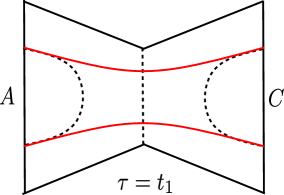
a)          b)    

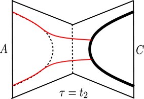
Figure 19: a) The connected entanglement wedge at $\tau=t_{1}$ where the minimal surface of $AC$ (shown in red) becomes comparable to those of $A$ and $C$. b) Locally accessible information satisfies $J^{W}(A:C)>0$ for $\tau>t_{2}>t_{1}$ where the minimal surface $\gamma_{A}$ of $A$ becomes comparable to the cross section $\Sigma_{A:B}$ of $A,B$.

5.2 Holographic scattering

Imagine that two signals travel to the center of the pure AdS₃, interact with each other, and scatter off to the boundary (Fig. 20(a)). Concretely, we arrange the input points $c_{1},c_{2}$ at $(\theta,t)=(-\pi/2,0),(\pi/2,0)$ and the output points $r_{1},r_{2}$ at $(\theta,t)=(0,\pi),(\pi,\pi)$, respectively as shown in Fig. 20(b). In this setup, while there is enough time for bulk scattering, there is not enough time for direct boundary scattering. Then, how does the interaction between two particles emerge on the boundary?

This apparent puzzle can be resolved by finding boundary spacetime regions which $c_{1}$ and $c_{2}$ can utilize [70]. Specifically, let us define

$$R_{1}\equiv J_{+}(c_{1})\cap J_{-}(r_{1})\cap J_{-}(r_{2}),\qquad R_{2}\equiv J_{+}(c_{2})\cap J_{-}(r_{1})\cap J_{-}(r_{2})$$ (166)

where $J_{+}$ and $J_{-}$ represent the future and past light cones respectively. These are the regions to which either one of the input signals has access and can signal to both of the output points. The crucial observation is that $R_{1}$ and $R_{2}$ have a connected entanglement wedge. This suggests a possibility that interactions between two particles occur indirectly by somehow utilizing the pre-shared entanglement due to the connected wedge. The proposal has been further strengthened; the bulk scattering in fact implies the connected entanglement wedge for $R_{1}$ and $R_{2}$, a result known as the connected wedge theorem [71, 72].

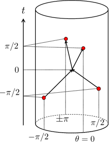
a)          b)    

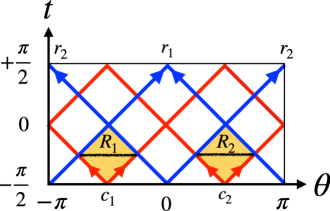
Figure 20: a) A bulk scattering process that cannot be realized as direct scattering on the boundary. b) The boundary causal structure. Interactions are induced by utilizing quantum entanglement shared between $R_{1}$ and $R_{2}$ due to the connected wedge.

In a series of works, May and collaborators have proposed several quantum information theoretic protocols that induce particular classes of interactions by using the pre-shared entanglement [70, 71, 72]. These protocols differ in details and purposes, but all of them utilize protocols similar to quantum teleportation, assuming access to clean EPR pairs that could hypothetically be distilled from $R_{1}$ and $R_{2}$ soon after their entanglement wedge becomes connected. (Note however that, in this regime, we have $J^{W}(R_{1}:R_{2})=0$ and thus, $E_{D}^{[\text{G-LOCC}]}\approx 0$ at the leading order.) Furthermore, we may note that these proposed protocols do not appear to work without (sufficiently) clean EPR pairs, at least in their original forms. Currently, it remains unclear whether the distillability of clean EPR pair is indeed a necessary condition for emerging interactions between particles in holography. If this turns out to be the case, the holographic scattering process suggests some mechanism, which is yet to be discovered, that gives rise to some corrections to our proposal of $E_{D}^{[\text{G-LOCC}]}\approx J^{W}(A:C)$. This may also be of interest as a purely quantum information theoretic question.

We however expect that such a process would make at most subleading contributions since the scattering process with $O(1/G_{N})$ entropy will induce significant backreaction to the geometry. For instance, the connected wedge theorem and related aspects have been studied for the conical defect and BTZ black hole geometries in [73]. One of their main findings is that loosely speaking, the bulk scattering process becomes harder to occur in these geometries.

5.3 Planck-scale effect

Finally, let us return to the original setup in Fig. 1, where $A$ and $C$ are separated by $B$ in the pure AdS₃. For large $B$, minimal surfaces $\gamma_{A},\gamma_{C}$ of $A,C$ are macroscopically separated in the AdS scale even if $A$ and $C$ have a connected wedge. In this case, we proposed $E_{D}^{[\text{LO}]}(A:C)\approx 0$ at the leading order. When $B$ becomes smaller and eventually empty, however, we will have $E_{D}^{[\text{LO}]}(A:C)\approx S_{A}$. This suggests that, as two minimal surfaces $\gamma_{A}$ and $\gamma_{C}$ approach, subleading corrections to $E_{D}^{[\text{LO}]}$ emerge and eventually become dominant.

We expect that this subleading effect becomes significant when $\gamma_{A}$ and $\gamma_{C}$ approaches at the Planck-scale. Namely, we find that $\rho_{AA^{\prime}}$ of the double-copy state, constructed from random tensor networks, can be approximated as a maximally mixed state that is prepared on the minimal surface of $AA^{\prime}$ or $BB^{\prime}$, while subleading corrections to $\rho_{AA^{\prime}}$ are exponentially suppressed with respect to $1/G_{N}$. When $\gamma_{A}$ and $\gamma_{C}$ are Planck-scale close to each other, these subleading terms become dominant and give rise to distillable entanglement between $A$ and $C$. A more detailed explanation is presented in Appendix D.

6 Beyond holographic measurement

In this section, we discuss whether LOCCs may outperform G-LOCCs in entanglement distillation or not.

6.1 Locally accessible information

We begin by studying locally accessible information $J^{G}(A|C)$ and $J(A|C)$. Namely, we propose that $J^{G}(A|C)$ and $J(A|C)$ match at the leading order

$$\boxed{\ J^{G}(A|C)\stackrel{{\scriptstyle?}}{{\approx}}J(A|C)\ }$$ (167)

suggesting that a maximal entropy drop $\Delta S_{A}$ can be achieved by holographic measurements on the minimal surface $\gamma_{C}$.

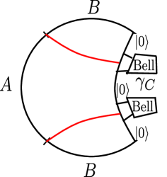
Figure 21: Bell measurements across the minimal cross section $\Sigma_{A:B}$. Measurements in entangled basis lead to larger $S_{A}^{\text{after}}$.

Generalized RT formula: The motivation behind this proposal comes from an observation that projections onto entangled states tend to increase $S_{A}^{\text{after}}$. Imagine that, instead of local product basis measurements, we perform Bell basis measurements that bridge the minimal cross section $\Sigma_{A:B}$, as depicted in Fig. 21. Then, $S_{A}^{\text{after}}$ will be larger due to extra Bell pairs shared between $A$ and $B$ in the post-measurement state. This can be understood naturally from the generalized RT formula. Let us interpret the minimal surface $\gamma_{C}$ as bulk DOFs encoded into boundary DOFs $A$ and $B$ via an isometric bulk-to-boundary map. If $|\psi_{C}\rangle$ is the post-measurement state on $\gamma_{C}$, the generalized RT formula predicts

$$S^{\text{after}}_{A}\approx E^{W}(A:B)+S_{C_{A}}(|\psi_{C}\rangle)$$ (168)

where $C_{A}$ is a subsystem located on $\gamma_{C}$ and lying inside the new entanglement wedge of $A$. The second term $S_{C_{A}}(|\psi_{C}\rangle)$ plays the role of the bulk entropy. This suggests that in maximizing the entropy drop $\Delta S_{A}$, projective measurements in a local basis on $\gamma_{C}$ will be optimal. One caveat in this argument is that the generalized RT formula is valid only when the bulk entropy is sub-leading. Indeed, there are known violations of the generalized RT formula when the bulk contribution becomes $O(1/G_{N})$ [61, 62]. It is however worth noting that in these examples, the bulk quantum states were chosen to be statistical mixtures (mixed states) of two states with distinct semiclassical duals. Here, we consider a projection onto a pure state. Also, note that placing a mixed state in the bulk increases the entropy whereas we seek the maximal entropy drop. For these reasons, we expect that our arguments are immune to adversarial constructions similar to the examples from  [61, 62].

Bulk causality: Another motivation behind this hypothesis is the emergent bulk causality. Since bulk DOFs in $\mathcal{E}_{AB}$ commute with those in $\mathcal{E}_{C}$ due to spacelike bulk separation, measurements on $C$ should not make any noticeable changes to bulk DOFs, including the metric components, in $\mathcal{E}_{AB}$. Suppose that $S_{A}$ drops to $S_{A}^{\text{after}}<E^{W}(A:B)$ due to some POVMs, and the minimal surface of $A$ becomes shorter than $E^{W}(A:B)$ at the leading order. This is likely to suggest that the geometry behind $\mathcal{E}_{C}$ (those inside $\mathcal{E}_{AB}$) has changed significantly due to backreaction by POVMs on $C$. This backreaction, however, is easily noticeable to bulk observers situated inside $\mathcal{E}_{AB}$, violating the bulk causality. As such, we expect that $S_{A}$ can drop at most to $S_{A}^{\text{after}}\approx E^{W}(A:B)$ at the leading order.

It is important to note that there may exist a projector $\Pi_{C}$ that leads to a post-measurement state with drastically modified geometry on $\mathcal{E}_{AB}$. For instance, in the thermofield double state, let us take $AB$ to be one side and $C$ to be the other side of the black hole. Projections onto a lower energy state on $C$ will result in a lower energy state on $AB$ as well, inducing significant change in the geometry. The probability amplitude of such projections, however, will be exponentially suppressed with respect to $1/G_{N}$. To be concrete, consider a POVM that projects $R$ onto either 1) a subspace spanned by the regularized boundary states $\{e^{-\alpha H/4}\ket{B_{a}}\}_{a}$, labeled as an outcome $0$, or 2) its orthogonal complement, labeled as an outcome $1$. If we apply this POVM on $R$ of a TFD state $\ket{\text{TFD}_{\beta}}\approx\sum_{n}\exp(-\beta E_{n}/2)\ket{n}_{L}\otimes\ket{n}_{R}$, the post-measurement state, corresponding to an outcome $0$, is given by $e^{-(\alpha+2\beta)H/4}\ket{B_{a}}_{L}$. This is dual to a one-sided black hole with the inverse temperature $2\beta+\alpha$ despite the entanglement wedge before the measurement was given by the right side of the two-sided black hole with the inverse temperature $\beta$. This measurement changes the geometry in the complementary entanglement wedge. However, the probability amplitude of obtaining such a state is exponentially suppressed, as explicitly verified in [74].

6.2 1WAY LOCC distillable entanglement

Finally, let us discuss 1WAY LOCC distillable entanglement. We claim that the proposed relation, $J^{G}(A|C)\approx J(A|C)$, implies

$$\boxed{\ E_{D}^{[\text{1WAY LOCC}]}(A:C)\approx J^{W}(A:C).\ }$$ (169)

This follows from a simple observation that one-shot 1WAY distillable entanglement is upper bounded by locally accessible information, namely

$$\boxed{\ E_{D}^{[\text{1WAY LOCC}](A\rightarrow C)}\leq J(C|A)\ }$$ (170)

on one-shot settings.

This can be proven as follows. Suppose $E_{D}^{[\text{1WAY LOCC}](A\rightarrow C)}>J(C|A)$. This suggests that some POVM acting on $A$, followed by LOs on $A$ and $C$, will distill $E_{D}^{[\text{1WAY LOCC}](A\rightarrow C)}$ EPR pairs. Here, we think of implementing LOs by using local unitary operations with additions of ancilla qubits, but without performing the trace operations. Note that omitting the trace operations does not affect the distillability of EPR pairs since EPR pairs will be prepared on qubits that are decoupled from DOFs that are to be traced out. This also ensures that LOs are unitary operations with additions of ancilla qubits, and thus do not change the entanglement entropy of $S_{C}$. As such, after performing this 1WAY LOCC entanglement distillation, the value of $S_{C}$ will stay the same or become smaller due to the POVM, on average. However, measuring distilled EPR pairs on $A$ can further decrease $S_{C}$ at least by $E_{D}^{[\text{1WAY LOCC}](A\rightarrow C)}$. This contradicts the fact that $J(C|A)$ is the maximal drop of $S_{C}$ due to POVMs on $A$. Hence, we must have $E_{D}^{[\text{1WAY LOCC}](A\rightarrow C)}\leq J(C|A)$.

6.3 Haar random state

Finally, let us recall some key results on $J(A|C)$ for Haar random states. A previous work [43] found that, when $n_{A},n_{B},n_{C}<\frac{n}{2}$, a Haar random state almost surely satisfies

$$J(A|C)\approx\max(n_{A}-n_{B},0).$$ (171)

Recall that, for a Haar random state, we have

$$E^{W}(A:B)\equiv\min\left({\begin{array}[]{c}\vbox{\vskip 6.0pt\hbox{\hskip 4.0pt\includegraphics[scale={2.0}]{fig_Haar_cross_A}}}\end{array}}\ {\begin{array}[]{c}\vbox{\vskip 6.0pt\hbox{\hskip 4.0pt\includegraphics[scale={2.0}]{fig_Haar_cross_B}}}\end{array}}\right)\ \approx\min(n_{A},n_{B})$$ (174)

and

$$J^{G}(A|C)\approx J^{W}(A|C)\equiv S_{A}-E^{W}(A:B)=\max(n_{A}-n_{B},0)$$ (175)

where $J^{G}(A|C)$ considers a random basis measurement on $C$. Hence, we find

$$\boxed{\ J^{G}(A|C)\approx J(A|C)\qquad\mbox{for Haar random states}.\ }$$ (176)

This suggests that the maximal average entropy drop can be achieved by a random measurement at the leading order. Furthermore, the observation from the previous subsection enables us to obtain the following result in one-shot settings:

$$\boxed{\ E_{D}^{[\text{1WAY LOCC}]}(A:C)\approx J(A:C)\qquad\mbox{for Haar random states}.\ }$$ (177)

These results provide further evidences supporting our proposals concerning $J(A|C)$ and $E_{D}^{[\text{1WAY LOCC}]}$ in holography.

7 Entanglement of formation

Our proposal, $J(A|C)\approx J^{W}(A|C)$, has a parallel statement for entanglement of formation $E_{F}(A:B)$ of a tripartite quantum state $|\psi_{ABC}\rangle$. Considering all the possible decompositions, $\rho_{AB}=\sum_{i}p_{i}|\psi_{i}\rangle\langle\psi_{i}|_{AB}$, $E_{F}(A:B)$ is given by the minimum of $\sum_{i}p_{i}S(\rho_{A}^{i})$. Moreover, the Koashi-Winter relation [34] relates $E_{F}(A:B)$ to locally accessible information $J(A|C)$:

$$J(A|C)=S_{A}-E_{F}(A:B).$$ (178)

Note that this is a quantum information theoretic identity, and is not specific to holography. Recalling $J^{W}(A|C)\equiv S_{A}-E_{W}(A:B)$, this suggests

$$\boxed{\ E_{F}(A:B)\approx E^{W}(A:B)\ }$$ (179)

at the leading order. An explicit form of $E^{W}(A:B)$ in the pure AdS₃ is given in Appendix A.

Our proposal of $J(A|C)\approx J^{W}(A|C)$ then implies that the optimal decomposition of $\rho_{AB}$ is given by the product-state basis along $\gamma_{C}$ as schematically shown below

$$|\psi_{AB}^{|0\rangle\dots|0\rangle}\rangle={\begin{array}[]{c}\vbox{\vskip 6.0pt\hbox{\hskip 4.0pt\includegraphics[scale={2.0}]{fig_decomposition}}}\end{array}}$$ (181)

Furthermore, assuming $J(A|C)\geq J(C|A)$ without loss of generality, we obtain a holographic monogamy relation

$$\boxed{\ E_{D}^{[\text{G-LOCC}]}(A:C)+E_{F}(A:B)\approx S_{A}.\ }$$ (182)

Furthermore, one can replace $E_{D}^{[\text{G-LOCC}]}(A:C)$ with $E_{D}^{[\text{1WAY LOCC}]}(A:C)$, conditioned on the proposal of $J(A|C)\approx J^{W}(A|C)$.

Finally, we note that Eq. (179) holds for a Haar random state since $J(A|C)\approx J^{W}(A|C)$ holds at the leading order as we explained in Section 6.3, based on the result from [43]. It then immediately follows from this result that

$$\boxed{\ E_{D}^{[\text{1WAY LOCC}]}(A:C)+E_{F}(A:B)\approx S_{A}\mbox{\quad for Haar random states.\quad}\ }$$ (183)

On Umemoto’s argument: In [15], Umemoto presented a no-go argument, suggesting $E_{F}\not=E^{W}$ in general. Here we discuss how our proposal circumvents it. Below, we begin by reproducing the argument as we understand it. Recall that entanglement of formation is upper bounded by $E_{F}(A:B)\leq\min(S_{A},S_{B})$. Also, recall the Araki-Lieb inequality

$$S_{A}+S_{AB}-S_{B}\geq 0.$$ (184)

These two bounds are related by the iff condition

$$E_{F}(A:B)=S_{A}\ \Leftrightarrow\ S_{A}+S_{AB}-S_{B}=0.$$ (185)

Suppose that $E_{F}(A:B)=E^{W}(A:B)$ to derive a contradiction. Umemoto pointed out that there are situations where

$$S_{A}+S_{AB}-S_{B}=O(1/G_{N})\quad\text{but}\quad E^{W}(A:B)=S_{A}.$$ (186)

This contradicts Eq. (185), suggesting $E_{F}(A:B)\not=E^{W}(A:B)$ in general.

This argument, however, can be circumvented if “$E_{F}=E^{W}$” is an equation at the leading order

$$S_{A}+S_{AB}-S_{B}=O(1/G_{N}),\qquad E_{F}(A:B)\approx E^{W}(A:B)=S_{A}.$$ (187)

We hasten to note that the possibility of subleading discrepancies was suggested in Umemoto’s work [15]. Here we would like to offer further insights into the origin of subleading contributions in light of our proposals. Concretely, when $ABC$ supports a pure state, the Araki-Lieb inequality is nothing but the non-negativity of the mutual information since $S_{A}+S_{AB}-S_{B}=I(A:C)$. Then the first of Eq. (187) suggests that $A,C$ have a connected wedge, and the second of Eq. (187) suggests $J(A|C)\approx 0$ at the leading order. This corresponds to the situation where $E_{D}^{[\text{G-LOCC}]}(A:C)\approx 0$ at the leading order while $I(A:C)=O(1/G_{N})$ (the regime II in Fig. 6). We have already alluded to potential physical mechanisms for subleading effects to $E_{D}^{[\text{G-LOCC}]}(A:C)$. While these observations on subleading effects primarily concern entanglement distillation, the same observation applies to $E_{F}(A:B)$ through the Koashi-Winter relation.

Violations for Rényi versions: Finally, we remark that the proposed duality in Eq. (179) does not hold for Rényi entropies. Namely, in Appendix C, D, we find that there exist regimes where

$$E_{F}^{(m)}(A:C)<E^{W}(A:C)\qquad m\geq 2$$ (188)

at the leading order, where the Rényi entanglement of formation $E_{F}^{(m)}$ is defined as the entanglement of formation with the entropy in the sum replaced by the Rényi-$m$ entropy. The decomposition basis to demonstrate this can be found by applying the Petz map to create the double-copy state and performing projective measurements on the second copy. The underlying mechanism for this deviation can be understood easily. As demonstrated in the next section, adding an exponentially small perturbation to separable state $\rho_{A}\otimes\rho_{A^{\prime}}$ can create large deviations between von Neumann quantities and Rényi quantities, and the double-copy state has this feature.

8 Bound entanglement in holography

One surprising aspect of our proposal is that there potentially exists a regime in holography where the mutual information $I(A:C)$ is large, but the G-LOCC distillable entanglement $E_{D}^{[\text{G-LOCC}]}$ may remain small. Such a regime typically arises right after the entanglement wedge becomes connected, but (gravitational) locally accessible information remains subleading.

Entangled states that are not distillable are often called bound entangled states in the quantum information literature and have been extensively studied [35]. Our proposal suggests a possibility that holographic states with a connected entanglement wedge may be examples of bound entangled states as

$$\boxed{\ E_{D}^{[\text{G-LOCC}]}(A:C)\approx 0<\frac{1}{2}I(A:C)<E_{F}(A:C)\approx E^{W}(A:C)\ }$$ (189)

under the hypothesis of $J(A:C)\approx J^{W}(A:C)$. (Here, $\frac{1}{2}I(A:C)$ in the middle comes from $E_{sq}$, see Eq. (17).) We, however, would like to emphasize that bound entanglement is conventionally discussed in asymptotic settings while our characterization concerns one-shot settings as inspired by quantum gravity considerations.

Holographic bound entanglement has been previously discussed in the literature. In particular, previous studies [75, 76] have found that, at finite temperature, there are states satisfying

$$E_{N}(A:B)\sim O(n),\qquad I(A:B)\sim o(n)$$ (190)

where $I(A:B)$ is sub-extensive in terms of the total number of qubits $n$. Here, $E_{N}$ denotes the logarithmic negativity, whose definition will be shortly given in Eq. (196). Note that distillable entanglement is upper bounded by $E_{N}$, namely $E_{D}\leq E_{N}$.

The authors of [75, 76] then proposed that extensive $E_{N}$ implies quantum entanglement in a sense of entanglement cost $E_{C}$. Recall that $E_{C}(A:B)$ corresponds to the number of EPR pairs per copy required to create $\rho_{AB}$ with an error vanishing at the asymptotic limit of a large number of copies. (It can be also defined as an asymptotic version of entanglement of formation $E_{F}$, and thus $E_{C}\leq E_{F}$.) While $E_{C}$ is difficult to estimate in general, a particular generalization of $E_{C}$ can be often analytically computed. Namely, the exact, positive partial transpose (PPT) entanglement cost $E_{C}^{[\mathrm{ppt,exact}]}$ is bounded below by $E_{N}$, $E_{C}^{[\mathrm{ppt,exact}]}\geq E_{N}$, as pointed out in [77]. Here, $E_{C}^{[\mathrm{ppt,exact}]}$ is defined as the number of EPR pairs per copy required to create the state in the asymptotic limit using the PPT-preserving operations with an exactly vanishing error before taking the asymptotic limit. Based on this observation, it has been proposed that a finite temperature state in a certain regime is an example of a bound entangled state since

$$E_{C}^{[\mathrm{ppt,exact}]}(A:B)\geq E_{N}(A:B)\sim O(n),\qquad E_{D}(A:B)\leq\frac{1}{2}I(A:B)\sim o(n).$$ (191)

At first slight, this proposal from [75, 76] might appear at odds with our proposal. Indeed, our claim was that bound entangled states may emerge in a regime with $I(A:C)\sim O(1/G_{N})$. On the contrary, the proposal from [75, 76] asserts that bound entangled states may emerge even when $I(A:C)\sim o(1/G_{N})$.

There are two potential scenarios to reconcile the tension between our proposal and theirs. First, our proposal is influenced by intuitions from Haar random states and tensors (as well as fixed-area states) where the entanglement spectrum is mostly flat. On the other hand, full holography exhibits a non-flat spectrum with Rényi entropy $S_{A}^{(m)}$ depending on $m$. This leaves a possibility that the non-flatness of the spectrum may be responsible for bound entanglement in the proposal from [75, 76]. Another potential resolution may be that $E_{C}$ and $E_{C}^{[\mathrm{ppt,exact}]}$ can be significantly different since $E_{C}^{[\mathrm{ppt,exact}]}$ requires an exact preparation of the state before taking the asymptotic limit. Indeed, this tends to be the case when there is an extensive deviation between the von Neumann entropy $S_{A}$ and Rényi entropy $S_{A}^{(m)}$. Below, we will illustrate this point concerning the subtle, yet crucial difference between $E_{C}$ and $E_{C}^{[\mathrm{ppt,exact}]}$ by studying the entanglement properties of an isotropic state.

8.1 Entanglement in isotropic state

An isotropic state is given by

$$\rho_{AA^{\prime}}=\frac{1-F}{{d_{A}}^{2}-1}(I-|\text{EPR}\rangle\langle\text{EPR}|)+F|\text{EPR}\rangle\langle\text{EPR}|,\quad 0\leq F\leq 1.$$ (192)

Recall that applying the Petz map to a Haar random state in a tripartition ($A,B,C$) and tracing out $B,B^{\prime}$ generate an approximation of this state when $n_{A}<n_{B}$. Namely, the EPR fidelity was given by

$$F\approx 2^{-\Delta}=\frac{d_{C}}{d_{A}d_{B}}\ll 1.$$ (193)

Note that we are interested in regimes where $\frac{n_{A}}{n},\frac{n_{B}}{n},\frac{n_{C}}{n}<\frac{1}{2}$ are held constant at the limit of large $n$.

Mutual information: We have $S_{A}=S_{A^{\prime}}=\log d_{A}$. As for $S_{AA^{\prime}}$, the following lower bound holds

$$\begin{split}S_{AA^{\prime}}&=-(d_{A}^{2}-1)\frac{1-F}{{d_{A}}^{2}-1}\log\frac{1-F}{{d_{A}}^{2}-1}-F\log F\\ &\geq(1-F)\log(d_{A}^{2}-1)=(1-F)\Big{(}2\log d_{A}+\log\big(1-\frac{1}{d_{A}^{2}}\big{missing})\Big{)}\\ &\geq(1-F)\Big{(}2\log d_{A}-\frac{1}{d_{A}^{2}-1}\Big{)}.\end{split}$$ (194)

Hence, we have $S_{AA^{\prime}}\approx 2\log d_{A}-2n_{A}F$ for small $F$, and

$$\boxed{\ I(A:A^{\prime})\approx 2n_{A}F\approx o(1)\ }$$ (195)

which is exponentially suppressed with respect to $n$.

Logarithmic negativity: The logarithmic negativity is defined as

$$E_{N}(A:A^{\prime})\equiv\log\quantity(\sum_{j}|\lambda_{j}|)$$ (196)

where $\lambda_{j}$ are eigenvalues of the partial transposed density matrix $\rho_{AA^{\prime}}^{T_{A^{\prime}}}$. For an isotropic state with small $F$, we find

$$\rho_{AA^{\prime}}^{T_{A^{\prime}}}\approx\frac{1}{{d_{A}}^{2}}I+F\frac{1}{d_{A}}\text{SWAP}$$ (197)

where the $\frac{1}{d_{A}}$ factor for SWAP comes from the normalization of $|\text{EPR}\rangle\langle\text{EPR}|$. The SWAP operator has $+1$ and $-1$ eigenvalues for symmetric states $|i,j\rangle+|j,i\rangle$) and anti-symmetric states ($|i,j\rangle-|j,i\rangle$). Hence $\rho_{AA^{\prime}}^{T_{A^{\prime}}}$ has the following eigenvalues:

$$\text{symmetric:}\ \frac{1}{d_{A}^{2}}\quantity(1+\frac{d_{C}}{d_{B}})\qquad\text{anti-symmetric:}\ \frac{1}{d_{A}^{2}}\quantity(1-\frac{d_{C}}{d_{B}}).$$ (198)

Let us focus on the regimes with $d_{C}\gg d_{B}$ (or equivalently $n_{C}>n_{B}$) where eigenvalues can be approximated as $\pm\frac{1}{d_{A}^{2}}\frac{d_{C}}{d_{B}}$. (Note that, for $d_{B}>d_{C}$, we have $E_{N}=0$.) We then have $\sum_{j}|\lambda_{j}|\approx\frac{d_{C}}{d_{B}}$. Hence we find

$$\boxed{\ E_{N}(A:A^{\prime})\approx\max(n_{C}-n_{B},0).\ }$$ (199)

Rényi entropy: The Rényi entropy $S_{AA^{\prime}}^{(m)}$ deviates significantly from the von Neumann entropy $S_{AA^{\prime}}^{(1)}$ as shown in Appendix C. Namely, we have

$$S_{AA^{\prime}}^{(m)}=\frac{1}{1-m}\Tr(\rho_{AA^{\prime}}^{m})\approx\frac{1}{m-1}\min(m\Delta,(m-1)2n_{A}).$$ (200)

where $\Delta=n_{A}+n_{B}-n_{C}$. For $m=2$, we have

$$S_{AA^{\prime}}^{(2)}=2(n_{A}+n_{B}-n_{C})\qquad\text{for $n_{C}>n_{B}$}$$ (201)

and thus, the (naïve un-sandwitched) Rényi-$2$ mutual information is

$$\frac{1}{2}I^{(2)}(A:A^{\prime})\approx n_{C}-n_{B}.$$ (202)

That this result matches with the value of $E_{N}(A:A^{\prime})$ is not a coincidence. As pointed out in [3, 78], the calculation of $E_{N}$ in holography is mostly controlled by the second, and more generally even-$m$ Rényi entropies.

Entanglement of formation: Analytical expressions of $E_{F}(A:A^{\prime})$ was obtained in [56, 79]:

$$E_{F}(A:A^{\prime})=\begin{cases}0,&F\in[0,1/d_{A}],\\ -(1-F)\frac{d_{A}}{d_{A}-2}\log(d_{A}-1)+\log d_{A},&F\in\left[\frac{4(d_{A}-1)}{d_{A}^{2}},1\right],\end{cases}$$

where $F=\frac{d_{C}}{d_{A}d_{B}}$. For small $F$, we find

$$\boxed{\ E_{F}(A:A^{\prime})\lesssim Fn_{A}\sim o(1)\ }$$ (203)

which is exponentially suppressed with respect to $n$.

8.2 Exact vs. approximate entanglement cost

When $n_{C}>n_{B}>n_{A}>0$ in the initial Haar random state, an isotropic state satisfies

$$I(A:A^{\prime})\sim o(1),\qquad E_{N}(A:A^{\prime})\approx n_{C}-n_{B},\qquad E_{C},E_{F}(A:A^{\prime})\sim o(1).$$ (204)

Here we used the fact that $E_{C}\leq E_{F}$ since $E_{C}$ can be defined as an asymptotic version of $E_{F}$. Recalling that $E_{C}^{[\text{exact}]}\geq E_{C}^{[\text{PPT exact}]}\geq E_{N}$ as LOCCs are a subset of PPT operations, we find

$$\boxed{\ E_{C}^{[\text{exact}]}\sim O(n),\qquad E_{C}\sim o(1)\ }$$ (205)

where $E_{C}$ is exponentially suppressed with respect to $n$. Hence, an isotropic state is not a bound entangled state in a sense of entanglement cost $E_{C}$ at the leading order in $n$.

In fact, one can verify that

$$E_{C}^{[\text{exact}]}\approx n_{C}-n_{B}.$$ (206)

To show this, note that $E_{C}^{[\text{exact}]}\geq E_{N}\gtrsim n_{C}-n_{B}$ from Eq. (204). Thus, we only need to show that $n_{C}-n_{B}$ EPR pairs are sufficient to create $\rho_{AA^{\prime}}$ with zero error. Let us prepare the following initial state on $AA^{\prime}$:

$$|0\rangle^{\otimes n_{A}+n_{B}-n_{C}}\otimes|\text{EPR}\rangle^{\otimes n_{C}-n_{B}}\otimes|0\rangle^{\otimes n_{A}+n_{B}-n_{C}}$$ (207)

where $n_{C}-n_{B}$ pairs of $|\text{EPR}\rangle$ is distributed between $A$ and $A^{\prime}$. Applying the two-fold Haar twirl from Eq. (74) generates $\rho_{AA^{\prime}}$ as it depolarizes all the states orthogonal to $|\text{EPR}\rangle_{AA^{\prime}}$. This verifies Eq. (206).

On the contrary, $E_{C}$ can be much smaller as it only requires approximate preparation with an asymptotically vanishing error. Namely, observing that $\rho_{AA^{\prime}}$ contains $|\text{EPR}\rangle_{AA^{\prime}}$ with $2^{-\Delta}$ probability, it suffices to prepare $\approx m2^{-\Delta}$ copies of $|\text{EPR}\rangle_{AA^{\prime}}$, and randomly distributing them over $m$ copies. (Note that this is essentially the same as how Shannon’s source coding works.) Namely, this method of randomly distributing EPR pairs over $m$ copies creates $\rho_{AA^{\prime}}^{\otimes m}$ with an error that vanishes at the limit of large $m$ due to the law of large numbers. But, this method does not create an exact $\rho_{AA^{\prime}}^{\otimes m}$ for any finite $m$. This needs only $\approx n_{A}2^{-\Delta}$ EPR pairs per copy. As such, we find

$$E_{C}\lesssim n_{A}2^{-\Delta}.$$ (208)

Here, to highlight the difference between exact and approximate preparations of states, we derived Eq. (206) and Eq. (208) by constructing explicit methods of creating $\rho_{AA^{\prime}}^{\otimes m}$ exactly and approximately. Note however that Eq. (208) follows straightforwardly from Eq. (203) as $E_{C}\leq E_{F}$ by definition.

Let us summarize the argument. For a finite temperature state with non-flat entanglement spectrum, the mutual information $\frac{1}{2}I(A:C)$ and the logarithmic negativity $E_{N}(A:C)$, which is dominated by Rényi-$2$ calculations, may have different transition points as pointed out in [75, 76]. The upshot of the above observation is that the deviation between mutual information $I(A:B)$ and logarithmic negativity $E_{N}(A:B)$ do not necessarily imply bound entanglement in a sense of $E_{C}$. Namely, adding a small (even exponentially small) perturbation to a separable state $\rho_{A}\otimes\rho_{C}$ suffices to create a large separation between $\frac{1}{2}I(A:C)$ and $E_{N}(A:C)$ as well as between $E_{C}$ and $E_{C}^{[\text{exact}]}$. To resolve this issue, careful analysis of $E_{F}$ or $E_{C}$ in full holography is needed, which we hope to provide in the future.

8.3 On NPT bound entanglement

Finally, let us comment on the problem concerning negative partial transpose (NPT) bound entanglement. A mixed state $\rho_{AC}$ is said to be an NPT state if the partial transpose $\rho_{AC}^{T_{C}}$ has a negative eigenvalue. Otherwise, the state is said to be a positive partial transpose (PPT) state. Here, it is useful to recall the Peres-Horodecki criterion for the separability of a mixed state:

$$\text{$\rho_{AC}$ is separable}\quad\Rightarrow\quad\text{$\rho_{AC}$ is a PPT state}.$$ (209)

Note that the converse statement is not true. Namely, there exist PPT states that are not separable. Such PPT states are examples of PPT bound entanglement states since $E_{D}(A:C)\leq E_{N}(A:C)=0$ for PPT states. A naturally arising question then concerns whether NPT bound entanglement states exist or not. To the best of our knowledge, this problem remains open. See [80] and [81] for the original discussion.

Our work provides an interesting perspective that holographic states may be examples of (a version of) NPT bound states. The logarithmic negativity $E_{N}(A:C)$ in random tensor networks is given by [3]

$$E_{N}(A:C)\approx\frac{1}{2}I(A:C).$$ (210)

This suggests that holographic states with a connected wedge are NPT states at the leading order since $E_{N}>0$ requires negative eigenvalues. We have shown that holographic states are not distillable under G-LOCCs at the leading order when $J^{W}(A:C)=0$. This suggests that there exist regimes where

$$E_{N}(A:C)\sim O(1/G_{N}),\qquad E_{D}^{[\text{G-LOCC}]}(A:C)\approx 0.$$ (211)

Whether a holographic state is an example of NPT bound states under generic LOCCs or not is an interesting open problem.

Meanwhile, as observed in Section 6.3, a Haar random state satisfies

$$E_{N}(A:C)\sim O(n),\qquad E_{D}^{[\text{1WAY LOCC}]}(A:C)\approx 0$$ (212)

in some regimes. Consequently, a Haar random state serves as an example of NPT bound entanglement at leading order in a sense of one-shot 1WAY LOCCs.

9 Outlook

Summary of proposals: Our main proposals can be summarized as follows.

• At the leading order, $E_{D}^{[\text{LO}]}(A:C)\approx 0$ when minimal surfaces $\gamma_{A},\gamma_{C}$ are spatially separated in the bulk.

• At the leading order, $E_{D}^{[\text{G-LOCC}]}(A:C)\approx J^{W}(A:C)\equiv S_{A}-E^{W}(A:B)$. Our 1WAY protocol is optimal under G-LOCCs. For Haar random states, this can be further strengthen to optimality under generic 1WAY LOCCs, showing the saturation of the hashing bound.

• Subleading contributions to these proposals may exist and play crucial roles in some dynamical phenomena.

In addition, based on physical arguments, we presented the following conjecture.

• Locally accessible information is given by $J(A:C)\approx J^{W}(A:C)$ at the leading order. Holographic measurements, placing EoW brane-like objects, achieve the maximal entropy drop.

Under this hypothesis, some of our claims may be strengthened as follows.

• At the leading order, $E_{D}^{[\text{1WAY LOCC}]}(A:C)\approx J^{W}(A:C)$ for holographic states.

• At the leading order, $E_{F}(A:C)\approx E^{W}(A:C)$ via the Koashi-Winter relation, but subleading corrections may (must) exist.

Some of the key implications of our proposals are summarized below.

• For holographic states with semiclassical duals, a connected entanglement wedges does not necessarily imply distillable entanglement.

• A leading-order NPT bound entanglement (in G-LOCC or 1WAY LOCC one-shot settings) exists in regimes where $I(A:C)\sim O(1/G_{N})$, but $J^{W}(A:C)\approx 0$. This typically occurs right after the entanglement wedge transition for the pure AdS₃.

Finally, let us highlight some of the technical novelties and their implications.

• We have demonstrated a method of bounding $E_{D}^{[\text{LO}]}$ by using the performance of the Petz recovery map. This provides an operational interpretation of entanglement wedge cross section $E^{W}$ and reflected entropy $S_{AA^{\prime}}$.

• We found that applying the Petz map to a Haar random state generates an isotropic state $\rho_{AA^{\prime}}$ when $n_{C}>n_{B}>n_{A}$.

Limitations and assumptions: It will be useful to summarize the limitations and assumptions associated with our claims. As for LO entanglement distillation, our technical results and assumptions are summarized as follows.

• For Haar random states, we argued $E_{D}^{[\text{LU}]}(A:C),E_{D}^{[\text{LO}]}(A:C)\approx 0$ based on a simple counting argument. We hope to present a rigorous version of this argument elsewhere. From the Petz map performance, we were only able to show $E_{D}^{[\text{LO}]}(A:C)\lesssim\min(\max(0,S_{A}-S_{AC}),\max(0,S_{C}-S_{AC}))$.

• For random tensor networks, we were only able to show $E_{D}^{[\text{LO}]}(A:C)\lesssim\min(J^{W}(A|C),J^{W}(C|A))$ from the Petz map performance.

• As an alternative evidence, we provided an interpretation of entanglement wedge reconstruction as LO entanglement distillation and showed that it implies $E_{D}^{[\text{LO}]}(A:C)\approx 0$ for spatially separated minimal surfaces. Namely, we assumed that entanglement wedge reconstruction applies to cases where bulk DOFs carry $O(1/G_{N})$ entropy. This assumption was proven in some particular regimes for random tensor networks.

• Random tensor networks suffer from a certain subtlety concerning the sub-AdS locality [18]. We implicitly discretized the static geometry down to a scale smaller than the AdS scale but larger than the Planck scale.

• To draw a conclusion concerning full holography, we implicitly assumed that the Petz map generates the double-copy geometry and that $S_{AA^{\prime}}$ is given by the RT surface at the leading order.

  These appear to be consistent with previous analyses as well as lessons on saddle points for higher Rényi calculations in random tensor networks [52, 53]. Also, see [82, 83] for potentially relevant studies.

As for G-LOCC entanglement distillation, our results rely on the following assumptions and are subject to some restrictions.

• We assumed that there exists a projective measurement basis in a subsystem $A$ that places EoW brane-like objects in $\mathcal{E}_{A}$. While this can be easily justified for random tensor network states, its validity in full holography remains to be verified.

• We were only able to show the optimality of our protocol under G-LOCCs. Combining with the proposal of $J(A|C)\approx J^{G}(A|C)$, we find that the protocol is optimal under 1WAY LOCCs. Based on the work [43], we verified that this is indeed the case for Haar random states.

Finally, for the subleading contributions, the following caveats should be emphasized.

• In the holographic task paradigm, previous works have provided lower bounds on mutual information only [70, 71, 72]. Whether the B₈₄ task and its variants also provide lower bounds on distillable entanglement remains open. Also, it remains open if bound (non-distillable) entanglement can assist some nonlocal quantum computational tasks.

• For traversable wormholes, it is unclear exactly at which $\tau$ entanglement distillation becomes possible. While previous works suggest that $\tau\sim t_{th}$ is sufficient, whether this occurs in regimes with $J^{W}(A:C)\approx 0$ or not remains to be verified.

Future problems: In addition to the aforementioned limitations and open problems, there are several important future problems.

• Much of our studies in the present paper focus on random tensor networks/fixed-area states. The most pressing future work is to verify our proposals in full holography, both from bulk quantum gravity and boundary CFT viewpoints.

• Do our proposals remain valid in the asymptotic settings? Some of our arguments, such as the upper bound on $E_{D}^{[\text{LO}]}(A:C)$ via the Petz recovery map, may apply to asymptotic settings as well.

• In defining $E_{D}$, we required that EPR pairs are prepared with an error $\epsilon$ which vanishes at the $G_{N}\rightarrow 0$ limit. This condition might look stronger than it should be, but this allowed us to obtain rigorous upper bounds on $E_{D}^{[\text{LO}]}$. Can this condition be relaxed?

  It should be also noted that entanglement distillation protocols with almost perfect fidelity exist in holography. Namely, the traversable wormhole teleportation fidelity (which can be interpreted as entanglement distillation fidelity) can approach unity in a certain limit [66]. While we expect that this only generates subleading contributions to $E_{D}^{[\text{LOCC}]}$, this work suggests that the condition of $\epsilon\rightarrow 0$ as $G_{N}\rightarrow 0$ may not be as demanding as it looks in holography.

• It is known that $E_{F}$ can violate the additivity relation by $O(1)$ amount [84]. But whether extensive violation is possible or not remains open. Can holography provide useful insights into the maximal possible additivity violation? See [85] also for some discussion in this direction, as well as a follow-up work [86].

• For holographic states (as well as Haar random states), there exists a regime with $E_{N}\sim O(1/G_{N})$ but $E_{D}^{[\text{G-LOCC}]}\approx 0$ at the leading order, suggesting that these are examples of approximately NPT bound entangled in one-shot, G-LOCC settings. Does this characterization extend to one-shot/asymptotic, LOCC settings?

• One natural generalization of our work is to consider restrictions on distillable entanglement in terms of quantum circuit complexity.

• Some of the techniques developed in this paper, such as the use of the Petz map to bound $E_{D}^{[\text{LO}]}$, may be useful in studying multipartite entanglement properties in various physical systems beyond the context of holography. One possible avenue is the Chern-Simons theory with boundaries. Another example is CFT (which is not necessarily holographic).

• Another potential avenue where our analyses may be applicable concerns random unitary quantum circuits and other related toy models of scrambling dynamics. On a related subject, our proposals about entanglement distillation may provide useful insights into how entanglement structure emerges in monitored (hybrid) quantum circuits where local projective measurements are added to dynamical many-body systems. Namely, projective measurements in such circuits exhibit a certain decoupling dynamics that is fundamentally akin to the information recovery in the Hayden-Preskill thought experiment [87]. Also, the effect of projective measurements on black holes was discussed in [88].

• We expect that our proposal concerning the shadow of entanglement wedge is likely to provide useful insights into DOFs behind the horizons, including the black hole interior and the spacetime outside the cosmological horizon [89, 90].

• Despite that a connected wedge does not necessarily guarantee distillable EPR pairs according to our proposal, it does not suggest any discontinuity of the spacetime within the entanglement wedge. We expect that a connected wedge is responsible for creating a smooth spacetime within an entanglement wedge where matter fields may move and interact with each other. Indeed, we proposed that traversable wormholes and holographic scattering may be examples of such phenomena enabled by a connected wedge. It will be interesting to verify these speculations by quantitative studies.

• It would be interesting to see if our proposal has something to say about the entanglement distillation process in the firewall thought experiment. Also, it would be interesting to explore the relation to the black hole interior and the role of observers [91, 92].

• Our proposals crucially rely on the assumption concerning the existence of disentangled basis states that may be associated with minimal surfaces. In order to put our arguments on firmer grounds, it is thus necessary to understand such disentangled basis states in terms of microstates in quantum gravity.

  Explicitly constructing such bulk disentangled states in concrete models of holography on the boundary, such as the Sachdev-Ye-Kitaev model, will be a useful first step to tackling this problem. It will be also interesting to address the entanglement distillation problems and related issues concerning disentangled states such as the distinguishability of black hole microstates through the lens of soft hairs.

Acknowledgment

We thank Hideo Furugori, Alex May, Yoshifumi Nakata, Tadashi Takayanagi, and Kotaro Tamaoka for helpful discussions. Research at Perimeter Institute is supported in part by the Government of Canada through the Department of Innovation, Science and Economic Development and by the Province of Ontario through the Ministry of Colleges and Universities. This work was supported by JSPS KAKENHI Grant Number 23KJ1154, 24K17047.

Appendix A $E_{D}^{\text{[G-LOCC]}}$ and $E_{F}$ for AdS₃/CFT₂

In the main body of the paper, we have claimed

$$E_{D}^{[\text{G-LOCC}]}(A:C)\approx\max(J^{W}(A|C),J^{W}(C|A)),$$ (213)

where

$$J^{W}(A|C)\equiv S_{A}-E^{W}(A:B),$$ (214)

and

$$E_{F}(A:C)\approx E^{W}(A:C).$$ (215)

In this appendix, we present calculations of $E^{W}(A:C)$ and $E^{W}(A:B)$ in the pure AdS₃. For simplicity, we set the AdS radius to be unity and focus on the case where $A$ and $C$ are two disjoint intervals, placed symmetrically on $S^{1}$. Namely, we take $A:[\frac{\pi}{2}-\frac{\theta}{2},\frac{\pi}{2}+\frac{\theta}{2}]$, $C:[-\frac{\pi}{2}+\frac{\theta}{2},-\frac{\pi}{2}-\frac{\theta}{2}]$ and $B$ to be their complement, where $\theta$ gives the angle of each subsystem. We will call two symmetric complementary subsystems as $B_{1}$ and $B_{2}$ as shown in Fig. 22.

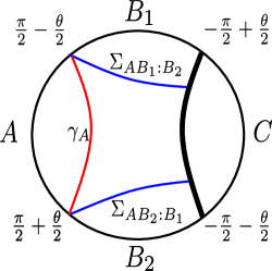
Figure 22: Two candidate configurations for $E^{W}(A:B)$ for two symmetric intervals $A$ and $C$ of angle $\theta$.

Let us begin with $E^{W}(A:C)$. Assume that the entanglement wedge is connected with $\theta>\frac{\pi}{2}$. (A disconnected wedge gives $E^{W}(A:C)=0$.) To compute the entanglement wedge cross section (Eq. (14)), we will need to evaluate the minimal cross-section $\Sigma_{A:C}$. It has been found that the cross section can be expressed as a function of the cross ratio $z$ [14]:

$$\text{Area}(\Sigma_{A:C})=\text{Cross}(z_{A:C})$$ (216)

where

$$\text{Cross}(z)\equiv\log(1+2z+2\sqrt{z(z+1)})\stackrel{{\scriptstyle z\gg 1}}{{\approx}}\frac{1}{4G_{N}}\log(4z).$$ (217)

Here, the cross ratio is given by

$$z_{A:C}=\frac{\displaystyle\sin\frac{\absolutevalue{A}}{2}\sin\frac{\absolutevalue{C}}{2}}{\displaystyle\sin\frac{\absolutevalue{B_{1}}}{2}\sin\frac{\absolutevalue{B_{2}}}{2}}=\tan^{2}\frac{\theta}{2}.$$ (218)

Hence, we have

$$\boxed{\ \begin{split}E^{W}(A:C)=\begin{cases}\displaystyle\frac{1}{4G_{N}}\log\quantity(1+2\tan^{2}\frac{\theta}{2}+2\frac{\tan\frac{\theta}{2}}{\cos\frac{\theta}{2}})\qquad\qquad&\frac{\pi}{2}\leq\theta\\ 0\qquad\qquad&\theta\leq\frac{\pi}{2}.\end{cases}\end{split}\ }$$ (219)

Next, let us compute $E^{W}(A:B)$. There are two possible candidate cross section surfaces for $E^{W}(A:B)$ as depicted in Fig. 22. The first candidate surface is given by the minimal surface $\gamma_{A}$:

$$\text{Area}(\gamma_{A})=2\log\frac{2\sin\frac{\theta}{2}}{\epsilon}$$ (220)

where we have introduced a UV cutoff $\epsilon$. The second candidate surface has two contributions which can be expressed as follows

$$\text{Area}(\Sigma_{AB_{2}:B_{1}})+\text{Area}(\Sigma_{AB_{1}:B_{2}}).$$ (221)

While $\text{Area}(\Sigma_{AB_{2}:B_{1}})$ is divergent, one can introduce a small UV cutoff angle $\epsilon$ between $AB_{2}$, and $B_{1}$. We then obtain

$$\text{Area}(\Sigma_{AB_{2}:B_{1}})=\text{Cross}(z_{AB_{2}:B_{1}})$$ (222)

where

$$z_{AB_{2}:B_{1}}=\frac{\displaystyle\sin\frac{\absolutevalue{AB_{1}}}{2}\sin\frac{\absolutevalue{B_{2}}}{2}}{\displaystyle\sin\frac{\absolutevalue{C}}{2}\sin{\epsilon}}\approx\frac{\cot\theta}{\epsilon}\gg 1.$$ (223)

Here we choose the same UV cutoff parameter $\epsilon$ as the one used for $\text{Area}(\gamma_{A})$ so that the following area difference remains finite

$$\text{Area}(\gamma_{A})-(\text{Area}(\Sigma_{AB_{2}:B_{1}})+\text{Area}(\Sigma_{AB_{1}:B_{2}})).$$ (224)

Hence, in a regime where the second candidate surface is dominant, we have

$$E^{W}(A:B)=\frac{2}{4G_{N}}\log(\frac{4\cot\theta}{\epsilon}).$$ (225)

and thus

$$\boxed{\ \begin{split}J^{W}(A:C)\equiv S_{A}-E^{W}(A:B)=\begin{cases}\displaystyle\frac{1}{2G_{N}}\log\frac{\sin\frac{\theta}{2}\tan\frac{\theta}{2}}{2},\qquad&\theta\geq\theta_{\ast}\\ 0\qquad&\theta\leq\theta_{\ast}\end{cases}\end{split}\ }$$ (226)

which is UV finite. Finally, the critical value $\theta=\theta_{\ast}$ when the G-LOCC distillable entanglement becomes nonzero at the leading order is found by

$$\text{Area}(\gamma_{A})=\text{Area}(\Sigma_{A:B})\Rightarrow\theta_{\ast}=4\mathrm{arctan}\sqrt{\sqrt{2}-1}\approx 2.287.$$ (227)

This completes the calculation of $\theta_{\ast}$ quoted in Fig. 6(b).

Appendix B Entanglement wedge transitions in a planar BTZ black hole

In this appendix, we present calculations of the transition times $t_{1}$ and $t_{2}$ for $I(A:C)$ and $J^{W}(A|C)$ in the BTZ black hole (see Fig. 19). This was mentioned in the context of traversable wormholes in Section 5.1.

Consider a thermofield double (TFD) state with the inverse temperature $\beta$ in $(1+1)$-dimensional holographic CFTs. The subsystems $A$ on the left boundary and $C$ on the right boundary are of equal size and grow linearly with the (one-sided) time, $\absolutevalue{A}=\absolutevalue{C}=2\tau$ after time $\tau$. In the case of the AdS₃/CFT₂, the gravity dual of the TFD state is described by the BTZ black hole. When the boundary topology is $\mathbb{R}^{1,1}$, the dual bulk metric is given by the planar BTZ black hole,

$$ds^{2}=\frac{1}{z^{2}}\quantity(-f(z)dt^{2}+dx^{2}+\frac{dz^{2}}{f(z)}),\quad f(z)=1-\frac{z^{2}}{z_{H}^{2}},$$ (228)

where the AdS radius is taken to be unity and the horizon radius is related to the inverse temperature by $z_{H}=\frac{\beta}{2\pi}$.

To calculate the transition time $t_{1},t_{2}$, it is convenient to introduce the embedding coordinates

$$\begin{split}X_{0}&=\frac{z_{H}}{z}\cosh\frac{x}{z_{H}},\\ X_{3}&=\sqrt{\quantity(\frac{z_{H}}{z})^{2}-1}\sinh\frac{t}{z_{H}},\\ X_{1}&=\frac{z_{H}}{z}\sinh\frac{x}{z_{H}},\\ X_{2}&=\sqrt{\quantity(\frac{z_{H}}{z})^{2}-1}\cosh\frac{t}{z_{H}}.\end{split}$$ (229)

One can reproduce the metric in Eq. (228) by plugging them in

$$ds^{2}=-dX_{0}^{2}-dX_{3}^{2}+dX_{1}^{2}+dX_{2}^{2}.$$ (230)

Using the embedding coordinates, the geodesic length between two bulk points $X_{A}$ and $X_{B}$ is given by

$$\mathrm{arccosh}\quantity(-X_{A}\cdot X_{B}),$$ (231)

where the inner product is defined as $X\cdot Y=-X_{0}Y_{0}-X_{3}Y_{3}+X_{1}Y_{1}+X_{2}Y_{2}$.

Using this formula, we can compute the geodesic lengths contributing to $I(A:C)$ and $J^{W}(A|C)$. Since we focus on a constant time slice, the RT formula suffices to compute entanglement entropy. Let us begin with $J^{W}(A|C)$. Recalling $J^{W}(A|C)\equiv S_{A}-E^{W}(A:B)$, we need to evaluate $E^{W}(A:B)$. There are two candidate surfaces. The first candidate $\frac{\text{Area}(\gamma_{A})}{4G_{N}}$ corresponds to the minimal surface of $A$. The second candidate $\frac{\text{Area}(\gamma_{A:B})}{4G_{N}}$ corresponds to the cross section with respect to $A,B$ where $B=(AC)^{c}$. When the subsystem size is $2\tau$, the lengths of two candidate geodesics are

$$\text{Area}(\gamma_{A}(\tau)) =2\log\frac{z_{H}}{\epsilon}+\log\quantity(2\cosh\frac{2\tau}{z_{H}}-2),$$ (232)

$$\text{Area}(\gamma_{A:B}(\tau)) =\min_{x_{H},x_{W}}\quantity[2\log\quantity(\frac{2z_{H}}{\epsilon}\cosh\frac{\tau-x_{H}}{z_{H}})+2\mathrm{arccosh}\quantity(\frac{\cosh\frac{\tau}{z_{H}}}{\sqrt{\cosh^{2}\frac{\tau}{z_{H}}-\cosh^{2}\frac{x_{W}}{z_{H}}}}\cosh\frac{x_{H}-x_{W}}{z_{H}})],$$ (233)

where $\epsilon(\ll 1)$ is the UV cutoff on the boundary. The second expression involves a minimization over $x_{H}$ and $x_{W}$, which are the $x$ coordinates at the intersection of the geodesic with the horizon or the edge of the complement entanglement wedge, respectively. See Fig. 23 for the illustration. Hence, $J^{W}(A|C)$ is given by

$$\begin{split}J^{W}(A|C)&=\frac{1}{4G_{N}}\big{[}\text{Area}(\gamma_{A}(\tau))-\min[\text{Area}(\gamma_{A}(\tau)),\text{Area}(\gamma_{A:B}(\tau))]\big{]}\\ &=\frac{1}{4G_{N}}\max\quantity[0,\text{Area}(\gamma_{A}(\tau))-\text{Area}(\gamma_{A:B}(\tau))].\end{split}$$ (234)

In the early time, $\text{Area}(\gamma_{A}(\tau))<\text{Area}(\gamma_{A:B}(\tau))$ and in the late time $\text{Area}(\gamma_{A}(\tau))>\text{Area}(\gamma_{A:B}(\tau))$. The transition happens when $\tau=t_{2}$ such that $\text{Area}(\gamma_{A}(t_{2}))=\text{Area}(\gamma_{A:B}(t_{2}))$. Since $\tau$ only appears with $z_{H}$, the transition time is $\tau\sim z_{H}$ (multiplied by the AdS radius). Numerically, we find

$$t_{2}\approx 0.21\beta.$$ (235)

Figure 23: The cross-section $\gamma_{A:B}$ before minimization. $x_{H},x_{W}$ are the $x$ coordinates on the horizon $z=z_{H}$ or the edge of the entanglement wedge of $C$, respectively.

As for $I(A:C)$, the length of the geodesics connecting $A$ and $C$ is

$$\text{Area}(\gamma_{AC}(\tau))=4\int_{\epsilon}^{z_{H}}\frac{1}{z}\quantity(1-\frac{z^{2}}{z_{H}^{2}})^{-1/2}=4\log\quantity(\frac{2z_{H}}{\epsilon}).$$ (236)

Note that this does not depend on $\tau$. The entanglement wedge between $A$ and $C$ has a transition at time $\tau=t_{1}$ such that $2\text{Area}(\gamma_{A}(t_{1}))=\text{Area}(\gamma_{AC})$. This again happens of order $\beta$ because

$$\cosh\frac{2t_{1}}{z_{H}}=\frac{3}{2}\Leftrightarrow t_{1}=\frac{z_{H}}{2}\mathrm{arccosh}\frac{3}{2}\approx 0.08\beta.$$ (237)

Appendix C Haar random double-copy state

This appendix is devoted to studies of entanglement properties of the double-copy state constructed from a Haar random state. Consider an $n$-qubit Haar random state $|\psi\rangle$ in a tripartition $ABC$. The number of qubits in each subsystem $R=A,B,C$ is denoted by $n_{R}$. We assume $n_{A},n_{B},n_{C}<\frac{n}{2}$, or equivalently $n_{A}<n_{B}+n_{C}$ and its permutations of subsystems. In this case, we have $I(A:C)\approx n_{A}+n_{C}-n_{B}\sim O(n)$, but $A,C$ are not maximally entangled, mimicking situations of our interest in holography. Applying the Petz recovery map on $C$ then creates the following double-copy state $|\Phi^{(\text{double})}_{ABA^{\prime}B^{\prime}}\rangle$:

$$|\Phi^{(\text{double})}_{ABA^{\prime}B^{\prime}}\rangle=\sqrt{d_{C}}\cdot{\begin{array}[]{c}\vbox{\vskip 6.0pt\hbox{\hskip 4.0pt\includegraphics[scale={2.0}]{fig_Haar_double}}}\end{array}}$$ (239)

with a normalization factor of $\sqrt{d_{C}}$. Here, the double-copy state can be constructed by preparing the second complex conjugate copy $|\psi^{*}\rangle_{A^{\prime}B^{\prime}C^{\prime}}$, and then $CC^{\prime}$ are projected onto EPR pairs. A surprising property of the Grover recovery protocol is that it creates a good approximation of $|\Phi^{(\text{double})}_{ABA^{\prime}B^{\prime}}\rangle$ unitarily without making use of any post-selection [47]. Note that approximation errors are suppressed exponentially with respect to $n$.

When $n_{C}>\frac{n}{2}$, the Petz recovery map distills nearly perfect EPR pairs on $AA^{\prime}$ and $BB^{\prime}$. Here we ask what kinds of quantum states we will obtain when $n_{C}<\frac{n}{2}$. The rest of this section is devoted to studying the double-copy state $|\Phi^{(\text{double})}_{ABA^{\prime}B^{\prime}}\rangle$, namely its reduced density matrix $\rho_{AA^{\prime}}$. The main claim of this section is

$$S_{AA^{\prime}}\approx\min\quantity({\begin{array}[]{c}\vbox{\vskip 0.59999pt\hbox{\hskip 0.4pt\includegraphics[scale={0.2}]{fig_SASAdouble-Haar}}}\end{array}}\,,{\begin{array}[]{c}\vbox{\vskip 0.59999pt\hbox{\hskip 0.4pt\includegraphics[scale={0.2}]{fig_SAAdouble-Haar}}}\end{array}})=2\min(n_{A},n_{B})$$ (242)

and thus

$$\frac{1}{2}I(A:A^{\prime})\approx\max(0,n_{A}-n_{B}).$$ (243)

Also, we find that $\rho_{AA^{\prime}}$ can be approximated as

$$\boxed{\ \rho_{AA^{\prime}}\approx 2^{-\Delta}|\text{EPR}\rangle\langle\text{EPR}|_{AA^{\prime}}+(1-2^{-\Delta})\mu_{\text{max}},\qquad\Delta=n_{A}+n_{B}-n_{C}>0\ }$$ (244)

where $\mu_{\text{max}}$ is a maximally mixed state on $AA^{\prime}$ for $n_{A}<n_{B}$, and is a maximally mixed state on some $d_{B}^{2}$-dimensional subspace of $AA^{\prime}$ for $n_{B}<n_{A}$. It is useful to expand $\rho_{AA^{\prime}}$ explicitly as

$$\rho_{AA^{\prime}}\approx 2^{-\Delta}|\text{EPR}\rangle\langle\text{EPR}|_{AA^{\prime}}+2^{-2n_{\min}}\sum_{j=1}^{2n_{\min}-1}|\psi_{j}\rangle\langle\psi_{j}|$$ (245)

where $n_{\min}\equiv\min(n_{A},n_{B})$, and $|\psi_{j}\rangle$’s are states orthogonal to $|\text{EPR}\rangle$. Since $2^{-\Delta}\gg 2^{-2n_{\min}}$ from $n_{A},n_{B}<n/2$, the spectrum of $\rho_{AA^{\prime}}$ consists of a single peak of $|\text{EPR}\rangle$ and a flat background with much smaller amplitudes as depicted in Fig. 10. While $|\text{EPR}\rangle_{AA^{\prime}}$ appears as the most probable state in $\rho_{AA^{\prime}}$, its probability amplitude is suppressed by $2^{-\Delta}$, suggesting that the Grover recovery protocol failed to distill EPR pairs.

When $\mu_{\text{max}}$ is a maximally mixed state on $AA^{\prime}$ (as in the $n_{A}<n_{B}$ cases), the quantum state in Eq. (244) is called isotropic states. It may be perplexing to find that $|\text{EPR}\rangle_{AA^{\prime}}$ can appear as the peak state even when $n_{C}<n_{A},n_{B}$. A key observation is that, when $n_{C}<n_{A},n_{B}$, the probability amplitude for $|\text{EPR}\rangle_{AA^{\prime}}$ becomes smaller. Indeed, isotropic states with $2^{-\Delta}<2^{-n_{A}}$ are known to be separable [56], which is the case when $n_{C}<n_{B}$. Hence, the appearance of $|\text{EPR}\rangle_{AA^{\prime}}$ as the peak state does not lead to entanglement between $AA^{\prime}$ in this regime. When $n_{B}<n_{A}$, $|\psi_{j}\rangle$’s in $\mu_{\text{max}}$ are some entangled states between $A$ and $A^{\prime}$, and thus $\mu_{\text{max}}$ may contain entanglement. Entanglement properties of $\mu_{\text{max}}$ in this regime remain unclear to us except that the mutual information is given by Eq. (243).

Before proceeding, we briefly remark on previous works. The spectral statistics of $\rho_{AA^{\prime}}$ (single peak with flat background) for a Haar random double-copy state has been identified in a series of works in the context of reflected entropies in holography [52, 53] and the Hayden-Preskill recovery problem [54]. That the peak state is given by $|\text{EPR}\rangle$ has not explicitly appeared in the literature to the best of our knowledge. Nevertheless, we emphasize that the analyses in this appendix should be viewed as a heuristic and simplified version of more complete and careful analyses from the previous works. Namely, to establish Eq. (244), one would need to analyze statistical variations of $\rho_{AA^{\prime}}$ which have been done in [52, 53].

C.1 Entanglement in double-copy state

Let us derive Eq. (244) by evaluating $\Tr[(\rho_{AA^{\prime}})^{m}\big{]}$ using the standard Haar calculus. See [28] for reviews. One can represent $\Tr[(\rho_{AA^{\prime}})^{m}\big{]}$ as

$$\Tr[(\rho_{AA^{\prime}})^{m}\big{]}\approx\ \frac{1}{{d_{C}}^{m}}{\begin{array}[]{c}\vbox{\vskip 0.93pt\hbox{\hskip 0.62pt\includegraphics[scale={0.31}]{fig_big_diagram}}}\end{array}}$$ (247)

Since $|\Phi^{(\text{double})}_{ABA^{\prime}B^{\prime}}\rangle$ contains $|\psi\rangle$ and $|\psi^{*}\rangle$, the calculation involves $2m$ copies of $|\psi\rangle$, and thus the $S_{2m}$ permutation group. Boundary conditions on $AA^{\prime},BB^{\prime},CC^{\prime}$ are given by

$$\Tr[(\rho_{AA^{\prime}})^{m}\big{]}:\ {\begin{array}[]{c}\vbox{\vskip 6.0pt\hbox{\hskip 4.0pt\includegraphics[scale={2.0}]{fig_Haar_boundary}}}\end{array}}$$ (249)

where $W_{o}$ is a cyclic permutation for $(1,3,\cdots,2m-1)$, $W_{e}$ is a reverse cyclic permutation for $(2,4,\cdots,2m)^{-1}$, and $W_{p}$ represents pairings (swaps), namely $W_{p}=(1,2)(3,4)\cdots(2m-1,2m)$.

The leading contribution will be given by a choice of $V\in S_{2m}$ that achieves the minimal cycle numbers (or the minimal energy associated with the $S_{2m}$ spin ferromagnet Hamiltonian). While all possible choices of $V$ make contributions to $\Tr[(\rho_{AA^{\prime}})^{m}\big{]}$, there are three important ones that result from $V=W_{o}W_{e},I,W_{p}$:

$$F_{\text{RT-$A$}}^{(m)}=2(m-1)n_{A},\phantom{-n_{C},}\qquad{\begin{array}[]{c}\vbox{\vskip 6.0pt\hbox{\hskip 4.0pt\includegraphics[scale={2.0}]{fig_Haar_RT_A}}}\end{array}}$$ (251)

$$F_{\text{RT-$B$}}^{(m)}=2(m-1)n_{B},\phantom{-n_{C},}\qquad{\begin{array}[]{c}\vbox{\vskip 6.0pt\hbox{\hskip 4.0pt\includegraphics[scale={2.0}]{fig_Haar_RT_B}}}\end{array}}$$ (253)

$$F_{\text{tri}}^{(m)}=m(n_{A}+n_{B}-n_{C}),\qquad{\begin{array}[]{c}\vbox{\vskip 6.0pt\hbox{\hskip 4.0pt\includegraphics[scale={2.0}]{fig_Haar_tri}}}\end{array}}$$ (255)

where we subtracted $mn_{c}$ which results from the normalization of $|\Phi^{(\text{double})}_{ABA^{\prime}B^{\prime}}\rangle$. The red cuts represent contributions with the specified boundary conditions and the blue cuts represent the normalization of $\rho_{AA^{\prime}}$ which is to be subtracted from the result. Hence we have

$$\Tr[(\rho_{AA^{\prime}})^{m}\big{]}=\frac{1}{2^{2(m-1)n_{A}}}+\frac{1}{2^{2(m-1)n_{B}}}+\frac{1}{2^{m(n_{A}+n_{B}-n_{C})}}+\cdots.$$ (256)

The first and second terms represent contributions analogous to the RT formula, evaluating minimal surfaces homologous to $AA^{\prime}$. In the regime of $n_{A},n_{B},n_{C}<\frac{n}{2}$, however, the third term, which we shall call the tripartite contribution, always becomes dominant for large $m$:

$$-\log\Tr[(\rho_{AA^{\prime}})^{m}\big{]}\approx m(n_{A}+n_{B}-n_{C})\qquad\mbox{for large $m$}.$$ (257)

Hence, we have

$$S_{AA^{\prime}}^{(m)}\approx n_{A}+n_{B}-n_{C}\qquad\mbox{for large $m$},$$ (258)

displaying a leading order deviation from the RT formula for Rényi entropy for large $m$.

As for the von Neumann entropy $S_{AA^{\prime}}$, recalling the formula for Rényi-$m$ entropy,

$$S_{AA^{\prime}}^{(m)}=-\frac{1}{m-1}\log\Tr[(\rho_{AA^{\prime}})^{m}\big{]}$$ (259)

we will need to evaluate the following contributions at the $m\rightarrow 1$ limit:

$$\lim_{m\rightarrow 1}\frac{F_{\text{RT-$A$}}^{(m)}}{m-1},\frac{F_{\text{RT-$B$}}^{(m)}}{m-1},\frac{F_{\text{tri}}^{(m)}}{m-1}.$$ (260)

We find that the tripartite contribution diverges due to the $1/(m-1)$ factor as $m\rightarrow 1$. Thus, the minimal contribution is always given by the RT contributions. Hence, we find

$$S_{AA^{\prime}}\approx\min\quantity({\begin{array}[]{c}\vbox{\vskip 0.59999pt\hbox{\hskip 0.4pt\includegraphics[scale={0.2}]{fig_SASAdouble-Haar}}}\end{array}}\,,{\begin{array}[]{c}\vbox{\vskip 0.59999pt\hbox{\hskip 0.4pt\includegraphics[scale={0.2}]{fig_SAAdouble-Haar}}}\end{array}})=2\min(n_{A},n_{B}).$$ (263)

From these results, one can estimate the probability spectrum of $\rho_{AA^{\prime}}$. Formally, this can be done by finding the moment generating function from $\log\Tr[(\rho_{AA^{\prime}})^{m}\big{]}$ and applying the inverse Laplace transformation. A useful rule of thumb is that $\log\Tr[(\rho_{AA^{\prime}})^{m}\big{]}$ being proportional to $m$ suggests the presence of a delta function in the probability distribution. One can then make the following ansatz

$$\rho_{AA^{\prime}}\approx 2^{-\Delta}|\Psi_{\text{max}}\rangle\langle\Psi_{\text{max}}|+(1-2^{-\Delta})\sigma,\qquad\Delta=n_{A}+n_{B}-n_{C}$$ (264)

where $|\Psi_{\text{max}}\rangle$ is some pure state and $\sigma$ is some mixed state.

One can further deduce the form of $\sigma$ by looking at the next leading contribution. Observe that $\Tr[(\rho_{AA^{\prime}})^{m}\big{]}$ has terms of the form $\frac{1}{2^{2(m-1)n_{A}}}$ and $\frac{1}{2^{2(m-1)n_{B}}}$ with a factor of $m-1$ in their exponents. Such contributions appear due to flat spectrum in some probability distribution. When $n_{A}<n_{B}$, we have $-\log\Tr[(\rho_{AA^{\prime}})^{m}\big{]}\approx m(n_{A}+n_{B}-n_{C})+2(m-1)n_{A}$ by including the next leading contribution. This suggests that $\sigma$ is simply a maximally mixed state on $AA^{\prime}$ On the other hand, when $n_{B}<n_{A}$, we have $-\log\Tr[(\rho_{AA^{\prime}})^{m}\big{]}\approx m(n_{A}+n_{B}-n_{C})+2(m-1)n_{B}$. This suggests that $\sigma$ is a maximally mixed state on some random $2^{2n_{B}}$-dimensional subspace of $AA^{\prime}$.

The remaining task is to find the expression of $|\Psi_{\text{max}}\rangle$. Our claim of $|\Psi_{\text{max}}\rangle\approx|\text{EPR}\rangle_{AA^{\prime}}$ can be supported by evaluating $\Tr[(\rho_{AA^{\prime}})^{m}|\text{EPR}\rangle\langle\text{EPR}|\big{]}\approx 2^{-m\Delta}$. The boundary conditions to evaluate it are given by

$$\Tr[\rho_{AA^{\prime}}^{m}|\text{EPR}\rangle\langle\text{EPR}|\big{]}:{\begin{array}[]{c}\vbox{\vskip 6.0pt\hbox{\hskip 4.0pt\includegraphics[scale={2.0}]{fig_Haar_boundary_EPR}}}\end{array}}$$ (266)

with an extra contribution of $-mn_{C}-n_{A}$ from normalizations. (Note that $-n_{A}$ results from $|\text{EPR}\rangle\langle\text{EPR}|$.) Here, $W_{\lambda}$ at $A$ is given the cyclic permutation in the diagram below:

$$\Tr[(\rho_{AA^{\prime}})^{m}\outerproduct{\text{EPR}}{\text{EPR}}\big{]}\approx\ \frac{1}{{d_{C}}^{m}d_{A}}{\begin{array}[]{c}\vbox{\vskip 6.0pt\hbox{\hskip 4.0pt\includegraphics[scale={2.0}]{fig_big_diagram_EPR}}}\end{array}}$$ (268)

There are several important contributions to consider, as listed below:

$$2(m-1)n_{A}:{\begin{array}[]{c}\vbox{\vskip 6.0pt\hbox{\hskip 4.0pt\includegraphics[scale={2.0}]{fig_Haar_boundary_EPR_A}}}\end{array}}$$ (270)

$$-n_{A}+(2m-1)n_{B}-n_{C}:{\begin{array}[]{c}\vbox{\vskip 6.0pt\hbox{\hskip 4.0pt\includegraphics[scale={2.0}]{fig_Haar_boundary_EPR_B}}}\end{array}}$$ (272)

$$2(m-1)n_{B}:{\begin{array}[]{c}\vbox{\vskip 6.0pt\hbox{\hskip 4.0pt\includegraphics[scale={2.0}]{fig_Haar_boundary_EPR_B2}}}\end{array}}$$ (274)

$$m(n_{A}+n_{B}-n_{C}):{\begin{array}[]{c}\vbox{\vskip 6.0pt\hbox{\hskip 4.0pt\includegraphics[scale={2.0}]{fig_Haar_boundary_EPR_tri}}}\end{array}}$$ (276)

The contribution from $V=W_{p}$ becomes dominant for large $m$. Hence we have

$$\Tr[\rho_{AA^{\prime}}^{m}|\text{EPR}\rangle\langle\text{EPR}|\big{]}\approx 2^{-m\Delta}.$$ (277)

We have numerically verified our claim, concerning the peak state being $|\text{EPR}\rangle$, as shown in Fig. 24. Specifically, we sampled a random tripartite state $V_{C^{\prime}\rightarrow AB}\ket{\text{EPR}}_{C^{\prime}C}$ where $V_{C^{\prime}\rightarrow AB}$ is a random isometry which maps the $d_{C}$-dimensional Hilbert space to the larger Hilbert space of dimension $d_{A}d_{B}$. Here, to reduce the computational cost, we used a random isometry $V$ instead of a Haar random state $|\psi_{ABC}\rangle$. (Note that the eigenvalues smaller than $10^{-15}$ are removed from the plot as these are likely to stem from precision errors.) The plots show the eigenvalue spectra of $\rho_{AA^{\prime}}$ and the entanglement fidelity of the eigenvector with the highest eigenvalue.

Fig. 24(a) shows the spectrum for a $12$-qubit random state where $(n_{A},n_{B},n_{C})=(3,4,5)$. In this regime with $n_{A}<n_{B}$, we expect that the resulting state $\rho_{AA^{\prime}}$ is close to an isotropic state, at least when we take the large system size limit while fixing the relative ratios among $(n_{A},n_{B},n_{C})$. Furthermore, since $n_{B}<n_{C}$, the state will be non-separable with $2^{-\Delta}>\frac{1}{d_{A}}$. We indeed found that the spectrum has a single peak and otherwise the spectrum is almost flat. Furthermore, the peak amplitude ($\approx 0.27$) is significantly larger than the background amplitudes ($\lesssim 0.03$), hinting that this is a non-separable state. Finally, the entanglement fidelity of the peak is indeed close to unity ($\approx 0.9896$), confirming our claim.

Fig. 24(b) shows the spectrum for a $11$-qubit random state where $(n_{A},n_{B},n_{C})=(2,5,4)$. In this regime, we expect that the resulting state $\rho_{AA^{\prime}}$ is still close to an isotropic state as $n_{A}<n_{B}$. But it will be separable with $n_{C}<n_{B}$ due to a smaller peak amplitude. We indeed found that the spectrum has a peak with the entanglement fidelity $0.9663$ and otherwise the spectrum is close to flat. However, as expected, we have a smaller amplitude of the EPR peak.

Finally, Fig. 24(c) shows the spectrum for a $9$ qubit random state where $(n_{A},n_{B},n_{C})=(3,4,2)$. In this regime, we expect to obtain an isotropic state with an even smaller peak as $n_{C}<n_{A},n_{B}$. The numerical result indeed shows a small peak. There are however a few features that appear to deviate from an isotropic state. First, we found that the rest of the spectrum is decaying slowly, rather than being flat. Additionally, the entanglement fidelity of the peak state is $\approx 0.5717$. These however may be due to finite size effects. For instance, the leading order estimate of the peak amplitude is $2^{-\Delta}=2^{-5}$ with $\Delta=n_{A}+n_{B}-n_{C}=5$ while the estimate of the background amplitude is $2^{-2n_{A}}=2^{-6}$.

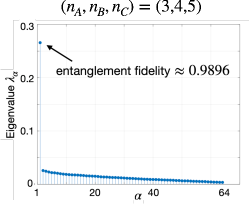
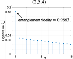
a)   b)   c)

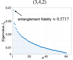
Figure 24: Spectra of the reduced density matrix $\rho_{AA^{\prime}}$ of the double-copy state and entanglement fidelities of the eigenstate with the highest eigenvalue.

C.2 Entanglement in post-measurement state

Next, we evaluate the entropy drop $\Delta S_{A}$ as a result of measuring $A^{\prime}$ in the double-copy state. Namely, we will demonstrate that our proposal of $E_{F}(A:C)\approx E^{W}(A:C)$ can be “violated” for Rényi-$m$ entropy for $m\geq 2$.

Letting $\rho_{A}^{\text{after}}$ be the post-measurement state on $A$, we begin by evaluating $\Tr\ [(\rho_{A}^{\text{after}})^{m}]$. Recall that the $m$-fold random projector can be written as a uniform sum of permutation operators:

$$\int d\psi\ |\psi\rangle\langle\psi|^{\otimes m}\propto\sum_{V\in S_{m}}V.$$ (278)

This suggests that, in the Haar calculus, random projections impose open boundary conditions. As such, the boundary conditions for computing $\Tr\ [(\rho_{A}^{\text{after}})^{m}]$ are given by

$$\Tr\ [(\rho_{A}^{\text{after}})^{m}]\ :\ {\begin{array}[]{c}\vbox{\vskip 6.0pt\hbox{\hskip 4.0pt\includegraphics[scale={2.0}]{fig_Haar_boundary_measure}}}\end{array}}$$ (280)

where an open boundary condition $O_{e}$ is imposed at $A^{\prime}$ (corresponding to even copies), in which an arbitrary permutation element can be chosen so that the domain wall energy becomes the lowest.

The important contributions are given by

$$F_{\text{RT-$A$}}^{(m)}=(m-1)n_{A},\phantom{-2n_{C},}\qquad{\begin{array}[]{c}\vbox{\vskip 6.0pt\hbox{\hskip 4.0pt\includegraphics[scale={2.0}]{fig_Haar_RT_A_measure}}}\end{array}}$$ (282)

$$F_{\text{RT-$B$}}^{(m)}=2(m-1)n_{B},\phantom{-n_{C},}\qquad{\begin{array}[]{c}\vbox{\vskip 6.0pt\hbox{\hskip 4.0pt\includegraphics[scale={2.0}]{fig_Haar_RT_B_measure}}}\end{array}}$$ (284)

$$F_{\text{tri}}^{(m)}=m(n_{A}+n_{B}-n_{C}),\qquad{\begin{array}[]{c}\vbox{\vskip 6.0pt\hbox{\hskip 4.0pt\includegraphics[scale={2.0}]{fig_Haar_tri_measure}}}\end{array}}$$ (286)

The first and second contributions represent the RT-like contributions. When $n_{C}>n_{B}$, the third term from the tripartite contribution becomes dominant at large $m$. Namely, we find

$$\boxed{\ \begin{split}S_{A}^{\text{after}(m)}\approx n_{A}+n_{B}-n_{C}\mbox{\quad when\quad}m>\frac{n_{A}}{n_{C}-n_{B}}>0\end{split}\ }$$ (287)

Since $n_{A}+n_{B}-n_{C}>0$ with $n_{C}>n_{B}$ implies $\frac{n_{A}}{n_{C}-n_{B}}>1$, the tripartite contribution dominates over the RT-like contributions for some $m$ larger than $1$. As $m\rightarrow 1$, however, the first and second terms always become more dominant. Hence, we have

$$\boxed{\ S_{A}^{\text{after}}\approx\min(n_{A},2n_{B}).\ }$$ (288)

Recalling Rényi versions of the Koashi-Winter relation [93], we obtain

$$\boxed{\ E_{F}^{(m)}(A:B)\lesssim S_{A}^{\text{after}(m)}.\ }$$ (289)

Hence, for $m\geq 2$, we have

$$\boxed{\ E_{F}^{(m)}(A:B)\lesssim\frac{m}{m-1}(n_{A}+n_{B}-n_{C})\leq 2(n_{A}+n_{B}-n_{C})\ }$$ (290)

$$\phantom{E_{F}^{(m)}(A:B)}\underset{m=\infty}{\longrightarrow}n_{A}+n_{B}-n_{C}.\phantom{\leq 2(n_{A}+n_{B}-n_{C})\qquad}$$

The upper bound can be smaller than $E^{W}(A:B)=\min(n_{A},2n_{B})$ at the leading order in some regimes.

Let us conclude by providing some numerical evidence. Given that the original state $\rho_{AA^{\prime}}$ is close to an isotropic state (for $n_{A}<n_{B}$), we expect that the spectrum of the post-measurement state has a similar form with a peak and a flat background. Fig. 25 shows a numerical calculation of the eigenvalue spectra of a typical post-measurement state. Here, a post-measurement state was obtained by $\Tr_{A^{\prime}}(\rho_{AA^{\prime}}\outerproduct{\psi}{\psi}_{A^{\prime}})$ up to normalization, where $\ket{\psi}$ is a random state drawn from Haar measure. Fig. 25(a) shows the case with $(n_{A},n_{B},n_{C})=(3,4,5)$ which exhibits a peak and otherwise a flat spectrum. Fig. 25(b) shows the same behavior but with a smaller amplitude of the peak. Finally, Fig. 25(c) shows a decaying spectrum where the peak behavior cannot be seen. These behaviors can be also understood by finding the explicit form of a post-measurement state by applying a projection on an isotropic state.

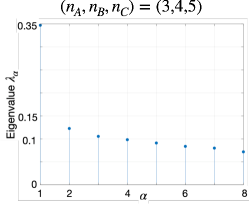
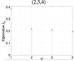
a)   b)   c)

Figure 25: Spectra of the reduced density matrix $\rho_{A}^{\text{after}}$ of the double-copy state after a random measurement on $A^{\prime}$. Note that each state corresponds to the respective state in Fig. 24 with the same label.

Appendix D Holographic double-copy state

In this section, we study the double-copy state for random tensor networks. We will focus on the following setup where two copies of the tensor network, the original $|\psi_{ABC}\rangle$ and the complex conjugated $|\psi_{ABC}^{*}\rangle$, are glued (contracted) at the minimal surface $\gamma_{C}$ of $C$:

$$|\psi_{ABC}\rangle={\begin{array}[]{c}\vbox{\vskip 6.0pt\hbox{\hskip 4.0pt\includegraphics[scale={2.0}]{fig_TN_original}}}\end{array}},\qquad|\Phi_{ABA^{\prime}B^{\prime}}^{(\text{double})}\rangle={\begin{array}[]{c}\vbox{\vskip 6.0pt\hbox{\hskip 4.0pt\includegraphics[scale={2.0}]{fig_TN_glue}}}\end{array}}\ .$$ (293)

Note that applying the Petz map on the boundary subsystem $C$ automatically coarse-grains the boundary DOFs into $\gamma_{C}$ as an approximate isometry is realized from $\gamma_{C}$ to $C$.

D.1 Entanglement in double-copy state

We begin by evaluating $\Tr[(\rho_{AA^{\prime}})^{m}\big{]}$. The boundary conditions are the same as in the case of Haar random states. For random tensor networks, each tensor in the bulk takes a spin value $V\in S_{2m}$ [28]. Here, we assume a tiling of Haar random tensors down to length scales shorter than the AdS scale, but larger than the Planck scale.

As before, we employ the folded geometry with $2m$ copies of $|\psi\rangle$ ($m$ copies of $|\psi\rangle$ and $|\psi^{*}\rangle$). Important contributions are listed below:

$$F_{\text{RT-$A$}}^{(m)}={\begin{array}[]{c}\vbox{\vskip 6.0pt\hbox{\hskip 4.0pt\includegraphics[scale={2.0}]{fig_TN_RT_A}}}\end{array}},\ F_{\text{RT-$B$}}^{(m)}={\begin{array}[]{c}\vbox{\vskip 6.0pt\hbox{\hskip 4.0pt\includegraphics[scale={2.0}]{fig_TN_RT_B}}}\end{array}},\ F_{\text{tri}}^{(m)}={\begin{array}[]{c}\vbox{\vskip 6.0pt\hbox{\hskip 4.0pt\includegraphics[scale={2.0}]{fig_TN_tri}}}\end{array}}$$ (297)

where we used $C$ to denote $\gamma_{C}$ for simplicity of notation. Note that $-m$ contribution on $C$ results from normalization. These diagrams result from placing spins $V=W_{o}W_{e},I,W_{p}$ in the bulk where their domain walls make energetic contributions to the effective ferromagnet Hamiltonian. The above diagrams make the following contributions:

$$\Tr[(\rho_{AA^{\prime}})^{m}\big{]}=2^{-F_{\text{RT-$A$}}^{(m)}}+2^{-F_{\text{RT-$B$}}^{(m)}}+2^{-F_{\text{tri}}^{(m)}}\cdots.$$ (298)

Note that while in principle all the possible spin configurations can make contributions to the computation of $\Tr[(\rho_{AA^{\prime}})^{m}\big{]}$, (one of) these three diagrams are expected to give rise to the leading order contributions to $\Tr[(\rho_{AA^{\prime}})^{m}\big{]}$.

The first and second contributions represent those analogous to the RT formula, evaluating the minimal surfaces of $AA^{\prime}$ in the glued geometry. For large $m$, the RT contribution asymptotes to geodesic lengths:

$$\frac{F_{\text{RT-$A$}}^{(m)}}{m-1}\underset{m=\infty}{\longrightarrow}\ {\begin{array}[]{c}\vbox{\vskip 6.0pt\hbox{\hskip 4.0pt\includegraphics[scale={2.0}]{fig_TN_RT_A_geo}}}\end{array}}={\begin{array}[]{c}\vbox{\vskip 6.0pt\hbox{\hskip 4.0pt\includegraphics[scale={2.0}]{fig_TN_glue_RT_A_geo}}}\end{array}}$$ (301)

$$\frac{F_{\text{RT-$B$}}^{(m)}}{m-1}\underset{m=\infty}{\longrightarrow}\ {\begin{array}[]{c}\vbox{\vskip 6.0pt\hbox{\hskip 4.0pt\includegraphics[scale={2.0}]{fig_TN_RT_B_geo}}}\end{array}}={\begin{array}[]{c}\vbox{\vskip 6.0pt\hbox{\hskip 4.0pt\includegraphics[scale={2.0}]{fig_TN_glue_RT_B_geo}}}\end{array}}$$ (304)

where we depicted the geodesics in both folded and unfolded glued geometries. The second diagram becomes dominant over the first one for $J^{W}(A|C)>0$ which is the regime when G-LOCC entanglement distillation becomes possible by measuring $C$. Namely, the smaller of Eq. (301) and Eq. (304) equals to $E^{W}(A:B)$.

The third contribution, which we shall call the tripartite contribution $F_{\text{tri}}^{(m)}$, can be found by choosing two interior vertices and constructing a tripartite diagram. (Note that two interior vertices may be placed on minimal surfaces $\gamma_{A},\gamma_{B},\gamma_{C}$, as well as on the asymptotic boundary. It is also possible to bring two vertices together. The diagram for $F_{\text{tri}}^{(m)}$ in Eq. (297) is one particular example of tripartite contributions. Also, note that the second RT diagram can be viewed as a particular case of the third diagram where inner vertices are placed on $\gamma_{C}$.) For large $m$, it asymptotes to

$$\frac{F_{\text{tri}}^{(m)}}{m-1}\ \underset{m=\infty}{\longrightarrow}\ {\begin{array}[]{c}\vbox{\vskip 6.0pt\hbox{\hskip 4.0pt\includegraphics[scale={2.0}]{fig_TN_RT_tri_geo}}}\end{array}}\ .$$ (306)

In the above diagram, we have not yet optimized the locations of two interior vertices to find the minimal configuration. We find that the minimal configuration for large $m$ can be constructed by further moving the interior vertices to the boundary, as schematically shown below

$${\begin{array}[]{c}\vbox{\vskip 6.0pt\hbox{\hskip 4.0pt\includegraphics[scale={2.0}]{fig_TN_RT_tri_geo}}}\end{array}}\ \geq\ {\begin{array}[]{c}\vbox{\vskip 6.0pt\hbox{\hskip 4.0pt\includegraphics[scale={2.0}]{fig_TN_RT_tri_geo_min}}}\end{array}},$$ (309)

which follows from the extremality of geodesics. As such, at $m\rightarrow\infty$, the tripartite contribution asymptotes to

$$\frac{F_{\text{tri}}^{(m)}}{m-1}\underset{m=\infty}{\longrightarrow}\ {\begin{array}[]{c}\vbox{\vskip 6.0pt\hbox{\hskip 4.0pt\includegraphics[scale={2.0}]{fig_TN_RT_tri_geo_min}}}\end{array}}\ .$$ (311)

We now show that the tripartite contribution is always dominant at large $m$ whenever $A$ and $C$ have connected wedges. Let us begin with the regime where the first RT contribution is dominant over the second RT contribution. We have

$${\begin{array}[]{c}\vbox{\vskip 6.0pt\hbox{\hskip 4.0pt\includegraphics[scale={2.0}]{fig_TN_RT_A_geo}}}\end{array}}\ -\ {\begin{array}[]{c}\vbox{\vskip 6.0pt\hbox{\hskip 4.0pt\includegraphics[scale={2.0}]{fig_TN_RT_tri_geo_min}}}\end{array}}\ ={\begin{array}[]{c}\vbox{\vskip 6.0pt\hbox{\hskip 4.0pt\includegraphics[scale={2.0}]{fig_TN_RT_AC_mutual}}}\end{array}}\ =I(A:C)>0$$ (315)

where the last inequality follows from the connected wedge with $I(A:C)=O(1/G_{N})$. Next, let us discuss the regime where the second RT contribution is dominant over the first RT contribution. We have

$$\begin{split}{\begin{array}[]{c}\vbox{\vskip 6.0pt\hbox{\hskip 4.0pt\includegraphics[scale={2.0}]{fig_TN_RT_B_geo}}}\end{array}}\ -\ {\begin{array}[]{c}\vbox{\vskip 6.0pt\hbox{\hskip 4.0pt\includegraphics[scale={2.0}]{fig_TN_RT_tri_geo_min}}}\end{array}}\ &=I(A:C)-2J^{W}(A|C)\geq 0.\end{split}$$ (316)

This inequality can be derived from two different arguments. First, it can be derived geometrically since Eq. (316) is equivalent to $E^{W}(A:B)\geq\frac{1}{2}I(A:B)$ [14]. Second, it can be also derived from an operational ground using our proposal. Namely, since one can LOCC distill at least $J^{W}(A|C)$ EPR pairs from $\rho_{AC}$, we must have $\frac{1}{2}I(A:C)\geq J^{W}(A|C)$.

To summarize, when $A,C$ have connected wedge with $I(A:C)\sim O(1/G_{N})$, we find

$$\boxed{\ S_{AA^{\prime}}^{(m)}\underset{m=\infty}{\longrightarrow}{\begin{array}[]{c}\vbox{\vskip 6.0pt\hbox{\hskip 4.0pt\includegraphics[scale={2.0}]{fig_TN_RT_tri_geo_min}}}\end{array}},\qquad\text{when $I(A:C)\sim O(1/G_{N})$ }\ .}$$ (318)

This demonstrates a leading order deviation from the RT formula for large $m$.

A similar violation of the RT formula occurs for Rényi-$2$ entropy as well. Here we will focus on the regime where the first RT contribution is dominant over the second one, namely $J^{W}(A|C)=0$. We will demonstrate that a leading order violation for $m=2$ occurs when $J^{W}(A|C)=0$, but $J^{W}(C|A)>0$. For $m=2$, the tripartite contribution is given by

$${\begin{array}[]{c}\vbox{\vskip 6.0pt\hbox{\hskip 4.0pt\includegraphics[scale={2.0}]{fig_TN_RT_tri_geo_m2}}}\end{array}}$$ (320)

where we have not yet optimized the locations of interior vertices for minimization in the above diagram. While we were not able to identify the global minimal configuration, we found the following candidate configuration:

$${\begin{array}[]{c}\vbox{\vskip 6.0pt\hbox{\hskip 4.0pt\includegraphics[scale={2.0}]{fig_TN_RT_tri_geo_m2_min}}}\end{array}}\geq\min F_{\text{tri}}^{(2)}$$ (322)

where two interior vertices are placed on $\gamma_{A}$. Below we demonstrate that there exists a regime where the above diagram is dominant over the first RT contribution. Observe

$${\begin{array}[]{c}\vbox{\vskip 6.0pt\hbox{\hskip 4.0pt\includegraphics[scale={2.0}]{fig_TN_RT_A_geo}}}\end{array}}-{\begin{array}[]{c}\vbox{\vskip 6.0pt\hbox{\hskip 4.0pt\includegraphics[scale={2.0}]{fig_TN_RT_tri_geo_m2_min}}}\end{array}}=2(S_{C}-E^{W}(B:C))=2J^{W}(C|A)$$ (325)

suggesting that, as long as $J^{W}(C|A)>0$, the tripartite contribution becomes dominant over the RT contributions. This provides us with an upper bound on the Rényi-$2$ entropy, and hence we have

$$\boxed{\ S_{AA^{\prime}}^{(2)}\approx\min F_{\text{tri}}^{(2)}\lesssim 2S_{A}-2J^{W}(C|A),\qquad\frac{1}{2}I^{(2)}(A:A^{\prime})\gtrsim J^{W}(C|A)\ }$$ (326)

where $I^{(2)}(A:A^{\prime})\equiv S_{A}^{(2)}+S_{A^{\prime}}^{(2)}-S_{AA^{\prime}}^{(2)}$ is a naïve Rényi-$2$ mutual information. Here, $S_{AA^{\prime}}^{(2)}$ deviates from the RT formula by at least $2J^{W}(C|A)$.

One interesting observation is that the (a)symmetry between $A$ and $C$ is closely related to the Rényi-$2$ entropy $S_{AA^{\prime}}^{(2)}$. Recall that we are considering a regime where $J^{W}(A|C)=0$ in the above discussion on $S_{AA^{\prime}}^{(2)}$. Here, Eq. (326) suggests that, when $S_{AA^{\prime}}^{(2)}\approx 2S_{A}$, we must have $J^{W}(C|A)=0$ as well. This suggests that G-LOCC distillable entanglement must be zero at the leading order as $J^{W}(A:C)\equiv\max(J^{W}(A|C),J^{W}(C|A))=0$.

As for the von Neumann entropy $S_{AA^{\prime}}$, recalling the formula for Rényi-$m$ entropy,

$$S_{AA^{\prime}}^{(m)}=-\frac{1}{m-1}\log\Tr[(\rho_{AA^{\prime}})^{m}\big{]}$$ (327)

we will need to evaluate the following contributions at the $m\rightarrow 1$ limit:

$$\lim_{m\rightarrow 1}\frac{F_{\text{RT}}^{(m)}}{m-1},\frac{F_{\text{tri}}^{(m)}}{m-1}.$$ (328)

We find that the tripartite diagram generates larger contributions due to the $1/(m-1)$ factor as $m\rightarrow 1$ unless the interior vertices exactly lie on $\gamma_{C}$, in which case the minimization gives the second RT contribution. Thus, the minimal configuration is always given by the RT contributions. Hence, we find

$$S_{AA^{\prime}}\approx\min\quantity({\begin{array}[]{c}\vbox{\vskip 6.0pt\hbox{\hskip 4.0pt\includegraphics[scale={2.0}]{fig_TN_RT_A_geo}}}\end{array}},\ {\begin{array}[]{c}\vbox{\vskip 6.0pt\hbox{\hskip 4.0pt\includegraphics[scale={2.0}]{fig_TN_RT_B_geo}}}\end{array}}).$$ (331)

Finally, let us briefly discuss potential subleading contributions to $\rho_{AA^{\prime}}$. For the double-copy state constructed from a Haar random state, we found that $\rho_{AA^{\prime}}$ consists of a single peak of $|\text{EPR}\rangle_{AA^{\prime}}$ and flat background distribution. In particular, this means that the state $\rho_{AA^{\prime}}$ can be approximated as a maximally mixed state on $AA^{\prime}$ (when $n_{A}<n_{B}$) with an exponentially small $2^{-\Delta}$ correction from $|\text{EPR}\rangle\langle\text{EPR}|_{AA^{\prime}}$. For random tensor networks, the above analyses suggest that $\rho_{AA^{\prime}}$ can be approximated as a maximally mixed state prepared on the minimal surface of $AA^{\prime}$ or $BB^{\prime}$ with some exponentially small corrections that consist of multiple different entangled states. Unfortunately, solving for full spectral properties appears challenging. Indeed, a tensor network state with just two tensors already exhibits surprising complexity in their entanglement properties [53]. Yet, one can still deduce (a part of) the spectrum and the contributing states by looking at the tripartite diagrams.

Here we will focus on contributions that result from the following diagram:

$${\begin{array}[]{c}\vbox{\vskip 6.0pt\hbox{\hskip 4.0pt\includegraphics[scale={2.0}]{fig_TN_tri_surface}}}\end{array}}$$ (333)

where two inner vertices are placed on $\gamma_{A}$. Looking at the scaling with respect to $m$, one can deduce that the following state contributes to $\rho_{AA^{\prime}}$:

$$2^{-\Delta}\cdot{\begin{array}[]{c}\vbox{\vskip 6.90001pt\hbox{\hskip 4.6pt\includegraphics[scale={2.3}]{fig_TN_tri_contribution}}}\end{array}}\qquad\Delta=\frac{1}{4G_{N}}{\begin{array}[]{c}\vbox{\vskip 6.0pt\hbox{\hskip 4.0pt\includegraphics[scale={2.0}]{fig_TN_tri_difference}}}\end{array}}$$ (336)

where $\Delta$ corresponds to the length difference between the red and blue curves, and the probability amplitude is exponentially suppressed with respect to $1/G_{N}$. Here $1/G_{N}$ should be understood as corresponding to local bond dimensions in tensor networks.

When $\gamma_{A},\gamma_{C}$ approach at the Planck scale, the length difference $\Delta$ will also be order of the Planck length. In such a regime, the correction terms become dominant.

D.2 Entanglement in post-measurement state

Next, let us study $J(A|C)$ and $E_{F}(A:B)$ by evaluating the entropy drop due to measuring $A^{\prime}$.

In the main text, we have seen that holographic (random projective) measurements lead to an entropy drop of $\Delta S_{A}\approx J^{W}(A:C)$. Here, we ask if further entropy drop may be possible or not by measuring $A^{\prime}$ in the double-copy state. A naïve intuition here would be that the Petz map (the Grover recovery) distills DOFs on $C$ which are strongly correlated with $A$. Then, by measuring $A^{\prime}$, the output of the Petz map, one might hope to decrease $S_{A}^{\text{after}}$ further. It turns out that this is not the case for von Neumann entropy $S_{A}^{\text{after}}$. But we will see that further entropy drop, larger than $J^{W}(A:C)$, is possible for Rényi-$m$ entropy $S_{A}^{(m)\text{after}}$. Namely, we demonstrate that our proposal of $E_{F}(A:B)\approx E^{W}(A:B)$ can be “violated” for Rényi-$m$ entropy, namely $E_{F}^{(m)}(A:B)\not\approx E^{W}(A:B)$ for large $m$ in general.

Let us discuss the effect of measuring the minimal surface of $A^{\prime}$ in the double-copy state $|\Phi\rangle$. Measuring $\gamma_{A}^{\prime}$ in a random basis places open boundary conditions along $\gamma_{A}^{\prime}$ (even copies of $A$). Important contributions are given by

$$F_{\text{RT-$A$}}^{\text{after}(m)}={\begin{array}[]{c}\vbox{\vskip 6.0pt\hbox{\hskip 4.0pt\includegraphics[scale={2.0}]{fig_TN_RT_A_after}}}\end{array}},\ F_{\text{RT-$B$}}^{\text{after}(m)}={\begin{array}[]{c}\vbox{\vskip 6.0pt\hbox{\hskip 4.0pt\includegraphics[scale={2.0}]{fig_TN_RT_B_after}}}\end{array}},\ F_{\text{tri}}^{\text{after}(m)}={\begin{array}[]{c}\vbox{\vskip 6.0pt\hbox{\hskip 4.0pt\includegraphics[scale={2.0}]{fig_TN_tri_after}}}\end{array}}$$ (340)

where open boundary conditions are shown in dotted green lines. We emphasize that the boundary spins $O_{e}$ along these lines cannot be placed beyond $\mathcal{E}_{A^{\prime}}$ since we perform measurements on $A^{\prime}$. For large $m$, these contributions asymptote to

$$\frac{F_{\text{RT-$A$}}^{\text{after}(m)}}{m-1}\rightarrow{\begin{array}[]{c}\vbox{\vskip 6.0pt\hbox{\hskip 4.0pt\includegraphics[scale={2.0}]{fig_TN_RT_A_geo_after}}}\end{array}}\!,\ \frac{F_{\text{RT-$B$}}^{\text{after}(m)}}{m-1}\rightarrow{\begin{array}[]{c}\vbox{\vskip 6.0pt\hbox{\hskip 4.0pt\includegraphics[scale={2.0}]{fig_TN_RT_B_geo_after}}}\end{array}}\!,\ \frac{F_{\text{tri}}^{\text{after}(m)}}{m-1}\rightarrow{\begin{array}[]{c}\vbox{\vskip 6.0pt\hbox{\hskip 4.0pt\includegraphics[scale={2.0}]{fig_TN_tri_geo_after}}}\end{array}}\!.$$ (344)

Let us focus on a regime where the first diagram is dominant over the second. In this regime, we find that the tripartite contribution becomes dominant over others at large $m$ when

$$J^{W}(C|A)>0.$$ (345)

To see this, observe

$${\begin{array}[]{c}\vbox{\vskip 6.0pt\hbox{\hskip 4.0pt\includegraphics[scale={2.0}]{fig_TN_RT_A_geo_after}}}\end{array}}-{\begin{array}[]{c}\vbox{\vskip 6.0pt\hbox{\hskip 4.0pt\includegraphics[scale={2.0}]{fig_TN_tri_geo_after}}}\end{array}}=J^{W}(C|A).$$ (348)

This suggests

$$E_{F}^{(m)}(A:B)<S_{A}-J^{W}(C|A)\mbox{\quad for large $m$.\quad}$$ (349)

Recalling that $E^{W}(A:B)=S_{A}-J^{W}(A|C)$, we find that

$$E_{F}^{(m)}(A:B)<E^{W}(A:B)\mbox{\quad for large $m$\quad}\quad\mbox{if $J^{W}(C|A)>J^{W}(A|C)$}.$$ (350)

Hence, we find that there exist regimes where $E_{F}^{(m)}(A:B)\not\approx E^{W}(A:B)$ for large $m$.

Finally, we discuss the effect of measuring both $A^{\prime}$ and $B^{\prime}$ in the double-copy state. In this case, one can in principle measure DOFs behind the minimal surface $\gamma_{A^{\prime}}$. Here, we focus on the following measurement pattern and the resulting tripartite contribution:

$$F_{\text{tri}}^{\text{after}(m)}\ =\ {\begin{array}[]{c}\vbox{\vskip 6.0pt\hbox{\hskip 4.0pt\includegraphics[scale={2.0}]{fig_TN_tri_after2}}}\end{array}}$$ (352)

where the measurement surface is shown in a dotted green line. Here the measurement surface can be placed beyond $\gamma_{A^{\prime}}$ as one has access to both $A^{\prime}B^{\prime}$. For large $m$, this asymptotes to

$$\frac{F_{\text{tri}}^{\text{after}(m)}}{m-1}\rightarrow{\begin{array}[]{c}\vbox{\vskip 6.0pt\hbox{\hskip 4.0pt\includegraphics[scale={2.0}]{fig_TN_tri_after2_geo}}}\end{array}}$$ (354)

This leaves a possibility of optimizing the locations of interior vertices and potentially further reducing $S_{A}^{\text{after}(m)}$ at large $m$. It is worth noting that this diagram is similar to the one studied in [82] (where $B$ was chosen to be a single interval as opposed to our case where $B$ consists of two intervals).

We conclude with one remark. Whether such tripartite contributions play significant roles in characterizing entanglement in $\rho_{AC}$ remains unclear at this moment. For one thing, tripartite contributions do not seem to survive at the $m\rightarrow 1$ limit for the same logic presented in the previous subsection, suggesting that these would make negligible (exponentially suppressed in $1/G_{N}$) perturbations only. In the main text, we highlighted a similar observation by studying the entanglement properties of the isotropic state. It should be, however, noted that there is a special way of taking the $m\rightarrow 1$ limit for a certain family of tripartite diagrams for which a smooth limit appears to exist [82]. Whether this particular procedure of taking the $m\rightarrow 1$ limit can be observed in robust entanglement measures or not remains to be seen.

References

- [1] L. Susskind, ER=EPR, GHZ, and the consistency of quantum measurements, Fortsch. Phys. 64 (2016) 72, [arXiv:1412.8483].
- [2] S. Nezami and M. Walter, Multipartite Entanglement in Stabilizer Tensor Networks, Phys. Rev. Lett. 125 (2020) 241602, [arXiv:1608.02595].
- [3] X. Dong, X.-L. Qi, and M. Walter, Holographic entanglement negativity and replica symmetry breaking, JHEP 06 (2021) 024, [arXiv:2101.11029].
- [4] C. Akers and P. Rath, Entanglement Wedge Cross Sections Require Tripartite Entanglement, JHEP 04 (2020) 208, [arXiv:1911.07852].
- [5] B. M. Terhal, M. Horodecki, D. W. Leung, and D. P. DiVincenzo, The entanglement of purification, J. Math. Phys. 43 (2002) 4286, [quant-ph/0202044].
- [6] C. H. Bennett, D. P. DiVincenzo, J. A. Smolin, and W. K. Wootters, Mixed state entanglement and quantum error correction, Phys. Rev. A 54 (1996) 3824, [quant-ph/9604024].
- [7] P. M. Hayden, M. Horodecki, and B. M. Terhal, The asymptotic entanglement cost of preparing a quantum state, J. Phys. A: Math. Gen. 34 (2001) 6891, [quant-ph/0008134].
- [8] M. Christandl and A. Winter, “squashed entanglement”: An additive entanglement measure, J. Math. Phys. 45 (2004) 829, [quant-ph/0308088].
- [9] E. M. Rains, A Rigorous treatment of distillable entanglement, Phys. Rev. A 60 (1999) 173, [quant-ph/9809078].
- [10] I. Devetak and A. Winter, Distillation of secret key and entanglement from quantum states, Proc. R. Soc. Lond. A 461 (2005) 207, [quant-ph/0306078].
- [11] M. Horodecki, P. Horodecki, and R. Horodecki, Unified approach to quantum capacities: Towards quantum noisy coding theorem, Phys. Rev. Lett. 85 (2000) 433.
- [12] P. Hayden, M. Headrick, and A. Maloney, Holographic Mutual Information is Monogamous, Phys. Rev. D 87 (2013) 046003, [arXiv:1107.2940].
- [13] P. Nguyen, T. Devakul, M. G. Halbasch, M. P. Zaletel, and B. Swingle, Entanglement of purification: from spin chains to holography, JHEP 01 (2018) 098, [arXiv:1709.07424].
- [14] T. Takayanagi and K. Umemoto, Entanglement of purification through holographic duality, Nature Phys. 14 (2018) 573, [arXiv:1708.09393].
- [15] K. Umemoto, Quantum and Classical Correlations Inside the Entanglement Wedge, Phys. Rev. D 100 (2019) 126021, [arXiv:1907.12555].
- [16] N. Cheng, Optimized Correlation Measures in Holography, Phys. Rev. D 101 (2020) 066009, [arXiv:1909.09334].
- [17] M. Miyaji and T. Takayanagi, Surface/State Correspondence as a Generalized Holography, PTEP 2015 (2015) 073B03, [arXiv:1503.03542].
- [18] N. Bao, G. Penington, J. Sorce, and A. C. Wall, Beyond Toy Models: Distilling Tensor Networks in Full AdS/CFT, JHEP 11 (2019) 069, [arXiv:1812.01171].
- [19] S. X. Cui, P. Hayden, T. He, M. Headrick, B. Stoica, and M. Walter, Bit Threads and Holographic Monogamy, Commun. Math. Phys. 376 (2019) 609, [arXiv:1808.05234].
- [20] M. Freedman and M. Headrick, Bit threads and holographic entanglement, Commun. Math. Phys. 352 (2017) 407, [arXiv:1604.00354].
- [21] M. Mezei and D. Stanford, On entanglement spreading in chaotic systems, JHEP 05 (2017) 065, [arXiv:1608.05101].
- [22] T. Takayanagi, Holographic Dual of BCFT, Phys. Rev. Lett. 107 (2011) 101602, [arXiv:1105.5165].
- [23] M. Fujita, T. Takayanagi, and E. Tonni, Aspects of AdS/BCFT, JHEP 11 (2011) 043, [arXiv:1108.5152].
- [24] T. Mori and B. Yoshida, Exploring causality in braneworld/cutoff holography via holographic scattering, JHEP 10 (2023) 104, [arXiv:2308.00739].
- [25] G. J. Galloway, K. Schleich, D. Witt, and E. Woolgar, The AdS / CFT correspondence conjecture and topological censorship, Phys. Lett. B 505 (2001) 255–262, [hep-th/9912119].
- [26] R. M. Wald, General Relativity. Chicago Univ. Pr., Chicago, USA, 1984.
- [27] F. Pastawski, B. Yoshida, D. Harlow, and J. Preskill, Holographic quantum error-correcting codes: Toy models for the bulk/boundary correspondence, JHEP 06 (2015) 149, [arXiv:1503.06237].
- [28] P. Hayden, S. Nezami, X.-L. Qi, N. Thomas, M. Walter, and Z. Yang, Holographic duality from random tensor networks, JHEP 11 (2016) 009, [arXiv:1601.01694].
- [29] A. Almheiri, Holographic Quantum Error Correction and the Projected Black Hole Interior, arXiv:1810.02055.
- [30] S. Antonini, G. Bentsen, C. Cao, J. Harper, S.-K. Jian, and B. Swingle, Holographic measurement and bulk teleportation, JHEP 12 (2022) 124, [arXiv:2209.12903].
- [31] W. H. Zurek, Quantum discord and maxwell’s demons, Phys. Rev. A 67 (2003) [quant-ph/0301127].
- [32] L. Henderson and V. Vedral, Classical, quantum and total correlations, J. Phys. A 34 (2001) 6899, [quant-ph/0105028].
- [33] P. Badziaa̧g, M. Horodecki, A. Sen(De), and U. Sen, Locally accessible information: How much can the parties gain by cooperating?, Phys. Rev. Lett. 91 (2003), no. 11 [quant-ph/0304040].
- [34] M. Koashi and A. Winter, Monogamy of quantum entanglement and other correlations, Phys. Rev. A 69 (2004) 022309, [quant-ph/0310037].
- [35] M. Horodecki, P. Horodecki, and R. Horodecki, Mixed state entanglement and distillation: Is there a ‘bound’ entanglement in nature?, Phys. Rev. Lett. 80 (1998) 5239, [quant-ph/9801069].
- [36] E. Lubkin, Entropy of an n-system from its correlation with a k-reservoir, J. Math. Phys. 19 (1978) 1028.
- [37] S. Lloyd and H. Pagels, Complexity as thermodynamic depth, Annals Phys. 188 (1988) 186.
- [38] D. N. Page, Average entropy of a subsystem, Phys. Rev. Lett. 71 (1993) 1291, [gr-qc/9305007].
- [39] D. Harlow, Jerusalem Lectures on Black Holes and Quantum Information, Rev. Mod. Phys. 88 (2016) 015002, [arXiv:1409.1231].
- [40] G. Aubrun, S. J. Szarek, and D. Ye, Entanglement thresholds for random induced states, Comm. Pure Appl. Math. 67 (2014) 129.
- [41] D. A. Roberts and B. Yoshida, Chaos and complexity by design, JHEP 04 (2017) 121, [arXiv:1610.04903].
- [42] E. Knill, Approximation by Quantum Circuits, quant-ph/9508006.
- [43] P. Hayden, D. W. Leung, and A. Winter, Aspects of generic entanglement, Comm. Math. Phys. 265 (2006) 95, [quant-ph/0407049].
- [44] H. Barnum and E. Knill, Reversing quantum dynamics with near-optimal quantum and classical fidelity, J. Math. Phys. 43 (2002) 2097, [quant-ph/0004088].
- [45] C.-F. Chen, G. Penington, and G. Salton, Entanglement Wedge Reconstruction using the Petz Map, JHEP 01 (2020) 168, [arXiv:1902.02844].
- [46] P. Hosur, X.-L. Qi, D. A. Roberts, and B. Yoshida, Chaos in quantum channels, JHEP 02 (2016) 004, [arXiv:1511.04021].
- [47] B. Yoshida and A. Kitaev, Efficient decoding for the Hayden-Preskill protocol, arXiv:1710.03363.
- [48] Y. Nakayama, A. Miyata, and T. Ugajin, The Petz (lite) recovery map for the scrambling channel, PTEP 2023 (2023) 123B04, [arXiv:2310.18991].
- [49] R. Li and J. Wang, Quantum information recovery from a black hole with a projective measurement, Phys. Rev. D 110 (2024) 026010, [arXiv:2401.14207].
- [50] A. Gilyén, S. Lloyd, I. Marvian, Y. Quek, and M. M. Wilde, Quantum Algorithm for Petz Recovery Channels and Pretty Good Measurements, Phys. Rev. Lett. 128 (2022) 220502, [arXiv:2006.16924].
- [51] T. Utsumi and Y. Nakata, Explicit decoders using quantum singular value transformation, arXiv:2405.06051.
- [52] C. Akers, T. Faulkner, S. Lin, and P. Rath, Reflected entropy in random tensor networks, JHEP 05 (2022) 162, [arXiv:2112.09122].
- [53] C. Akers, T. Faulkner, S. Lin, and P. Rath, Reflected entropy in random tensor networks. Part II. A topological index from canonical purification, JHEP 01 (2023) 067, [arXiv:2210.15006].
- [54] B. Czech, S. Shuai, and H. Tang, Entropies and reflected entropies in the Hayden-Preskill protocol, JHEP 02 (2024) 040, [arXiv:2310.16988].
- [55] S. Dutta and T. Faulkner, A canonical purification for the entanglement wedge cross-section, JHEP 03 (2021) 178, [arXiv:1905.00577].
- [56] B. M. Terhal and K. G. H. Vollbrecht, Entanglement of formation for isotropic states, Phys. Rev. Lett. 85 (2000) 2625, [quant-ph/0005062].
- [57] K. Fang, X. Wang, M. Tomamichel, and R. Duan, Non-asymptotic entanglement distillation, IEEE Transactions on Information Theory 65 (2019), no. 10 6454.
- [58] T.-C. Lu and T. Grover, Entanglement transitions as a probe of quasiparticles and quantum thermalization, Phys. Rev. B 102 (2020) 235110, [arXiv:2008.11727].
- [59] C. H. Bennett, D. P. DiVincenzo, J. A. Smolin, and W. K. Wootters, Mixed-state entanglement and quantum error correction, Phys. Rev. A 54 (1996) 3824.
- [60] A. Almheiri, X. Dong, and D. Harlow, Bulk Locality and Quantum Error Correction in AdS/CFT, JHEP 04 (2015) 163, [arXiv:1411.7041].
- [61] C. Akers and G. Penington, Leading order corrections to the quantum extremal surface prescription, JHEP 04 (2021) 062, [arXiv:2008.03319].
- [62] C. Akers, S. Leichenauer, and A. Levine, Large Breakdowns of Entanglement Wedge Reconstruction, Phys. Rev. D 100 (2019) 126006, [arXiv:1908.03975].
- [63] V. Balasubramanian, B. D. Chowdhury, B. Czech, and J. de Boer, Entwinement and the emergence of spacetime, JHEP 01 (2015) 048, [arXiv:1406.5859].
- [64] P. Gao, D. L. Jafferis, and A. C. Wall, Traversable Wormholes via a Double Trace Deformation, JHEP 12 (2017) 151, [arXiv:1608.05687].
- [65] J. Maldacena, D. Stanford, and Z. Yang, Diving into traversable wormholes, Fortsch. Phys. 65 (2017) 1700034, [arXiv:1704.05333].
- [66] P. Gao and D. L. Jafferis, A traversable wormhole teleportation protocol in the SYK model, JHEP 07 (2021) 097, [arXiv:1911.07416].
- [67] A. R. Brown, H. Gharibyan, S. Leichenauer, H. W. Lin, S. Nezami, G. Salton, L. Susskind, B. Swingle, and M. Walter, Quantum Gravity in the Lab. I. Teleportation by Size and Traversable Wormholes, PRX Quantum 4 (2023) 010320, [arXiv:1911.06314].
- [68] S. Nezami, H. W. Lin, A. R. Brown, H. Gharibyan, S. Leichenauer, G. Salton, L. Susskind, B. Swingle, and M. Walter, Quantum Gravity in the Lab. II. Teleportation by Size and Traversable Wormholes, PRX Quantum 4 (2023) 010321, [arXiv:2102.01064].
- [69] T. Schuster, B. Kobrin, P. Gao, I. Cong, E. T. Khabiboulline, N. M. Linke, M. D. Lukin, C. Monroe, B. Yoshida, and N. Y. Yao, Many-Body Quantum Teleportation via Operator Spreading in the Traversable Wormhole Protocol, Phys. Rev. X 12 (2022) 031013, [arXiv:2102.00010].
- [70] A. May, Quantum tasks in holography, JHEP 10 (2019) 233, [arXiv:1902.06845]. [Erratum: JHEP 01, 080 (2020)].
- [71] A. May, G. Penington, and J. Sorce, Holographic scattering requires a connected entanglement wedge, JHEP 08 (2020) 132, [arXiv:1912.05649].
- [72] A. May, J. Sorce, and B. Yoshida, The connected wedge theorem and its consequences, JHEP 11 (2022) 153, [arXiv:2210.00018].
- [73] J. Caminiti, B. Friedman-Shaw, A. May, R. C. Myers, and O. Papadoulaki, Holographic scattering and non-minimal RT surfaces, arXiv:2404.15400.
- [74] M. Miyaji, T. Takayanagi, and T. Ugajin, Spectrum of End of the World Branes in Holographic BCFTs, JHEP 06 (2021) 023, [arXiv:2103.06893].
- [75] S. Vardhan, J. Kudler-Flam, H. Shapourian, and H. Liu, Mixed-state entanglement and information recovery in thermalized states and evaporating black holes, JHEP 01 (2023) 064, [arXiv:2112.00020].
- [76] S. Vardhan, J. Kudler-Flam, H. Shapourian, and H. Liu, Bound Entanglement in Thermalized States and Black Hole Radiation, Phys. Rev. Lett. 129 (2022) 061602, [arXiv:2110.02959].
- [77] K. Audenaert, M. B. Plenio, and J. Eisert, Entanglement cost under positive-partial-transpose-preserving operations, Phys. Rev. Lett. 90 (2003) [quant-ph/0207146].
- [78] X. Dong, J. Kudler-Flam, and P. Rath, Entanglement Negativity and Replica Symmetry Breaking in General Holographic States, arXiv:2409.13009.
- [79] Y.-X. Wang, L.-Z. Mu, V. Vedral, and H. Fan, Entanglement Rényi entropy, Phys. Rev. A 93 (2016) 022324.
- [80] D. P. DiVincenzo, P. W. Shor, J. A. Smolin, B. M. Terhal, and A. V. Thapliyal, Evidence for bound entangled states with negative partial transpose, Phys. Rev. A 61 (2000) [quant-ph/9910026].
- [81] W. Dür, J. I. Cirac, M. Lewenstein, and D. Bruß, Distillability and partial transposition in bipartite systems, Phys. Rev. A 61 (2000) [quant-ph/9910022].
- [82] G. Penington, M. Walter, and F. Witteveen, Fun with replicas: tripartitions in tensor networks and gravity, JHEP 05 (2023) 008, [arXiv:2211.16045].
- [83] J. Harper, T. Takayanagi, and T. Tsuda, Multi-entropy at low Renyi index in 2d CFTs, SciPost Phys. 16 (2024) 125, [arXiv:2401.04236].
- [84] M. B. Hastings, Superadditivity of communication capacity using entangled inputs, Nature Phys. 5 (2009) 255.
- [85] P. Hayden and G. Penington, Black hole microstates vs. the additivity conjectures, arXiv:2012.07861.
- [86] Z. Wei and Y. Yoneta, Counting atypical black hole microstates from entanglement wedges, JHEP 05 (2024) 251, [arXiv:2211.11787].
- [87] B. Yoshida, Decoding the Entanglement Structure of Monitored Quantum Circuits, arXiv:2109.08691.
- [88] B. Yoshida, Projective measurement of black holes, arXiv:2203.04968.
- [89] V. Franken and T. Mori, Horizon causality from holographic scattering in asymptotically dS3, arXiv:2410.09050.
- [90] E. Shaghoulian and L. Susskind, Entanglement in De Sitter space, JHEP 08 (2022) 198, [arXiv:2201.03603].
- [91] B. Yoshida, Firewalls vs. Scrambling, JHEP 10 (2019) 132, [arXiv:1902.09763].
- [92] B. Yoshida, Observer-dependent black hole interior from operator collision, Phys. Rev. D 103 (2021) 046004, [arXiv:1910.11346].
- [93] T. Debarba, Koashi-Winter relation for -Renyi entropies, arXiv:1706.01924.