A robust first order meshfree method for
time-dependent nonlinear conservation laws

Abstract.

We introduce a robust first order accurate meshfree method to numerically solve time-dependent nonlinear conservation laws. The main contribution of this work is the meshfree construction of first order consistent summation by parts differentiations. We describe how to efficiently construct such operators on a point cloud. We then study the performance of such differentiations, and then combine these operators with a numerical flux-based formulation to approximate the solution of nonlinear conservation laws, with focus on the advection equation and the compressible Euler equations. We observe numerically that, while the resulting mesh-free differentiation operators are only $O(h^{\frac{1}{2}})$ accurate in the $L^{2}$ norm, they achieve $O(h)$ rates of convergence when applied to the numerical solution of PDEs.

1   Introduction

Numerical methods for solving partial differential equations (PDEs) form the backbone of computational modeling and simulation efforts in science and engineering. The majority of numerical methods for PDEs rely on a representation of the domain as a mesh. However, solution quality and mesh quality are strongly related, such that poor quality meshes with irregularly shaped elements result in poorly approximated solutions [1, 27, 16]. This is especially problematic in 3D, where it is difficult to automatically and efficiently generate unstructured meshes with guaranteed element quality [4].

Meshfree methods encompass a broad class of numerical schemes intended to circumvent the mesh generation step. These methods range from particle-based methods to high order collocation type schemes [10]. However, a common issue faced by meshfree discretizations is balancing accuracy with stability and robustness. While there are a variety of methods for constructing accurate structure preserving mesh-based discretiztations [9, 21, 7], it is more difficult to ensure that meshfree methods are conservative and stable [28, 11].

In this paper, we present a method for constructing meshfree discretizations based on the enforcement of a summation-by-parts (SBP) property. This work is closely related to the formulation of [5], but exploits the fact that enforcing only first order accuracy constraints results in a simpler construction of meshfree operators [32]. These operators are then used to formulate a meshfree semi-discretization in terms of finite volume fluxes, as is done in [5]. If these fluxes are local Lax-Friedrichs fluxes with appropriate wave-speed estimates, the resulting discretization can be shown to be invariant-domain preserving under forward Euler time-stepping and a CFL condition.

The paper proceeds as follows. In Section 2, we introduce the concept of summation by parts (SBP) operators. In Section 3, we introduce a methodology for constructing SBP and norm matrices given a point cloud, an adjacency matrix, and surface information (e.g., outward unit normals and boundary quadrature weights). In Section 4, we explore different ways of constructing the adjacency matrix and its effect on the behavior of the differentiation matrix. In Section 5, we discuss how to construct a numerical method for nonlinear conservation laws based on the meshfree operators, and in Section 6, we present some numerical results where we apply the method to the 2D linear advection and compressible Euler equations.

2   Summation by parts operators

The goal of this paper is to create a first order accurate meshless numerical method to solve non-linear conservation laws. The main tool in building such a numerical method will be summation by parts differentiation operators. Such methods are useful for constructing numerical discretizations which are both conservative and satisfy an energetic or entropic statement of stability [5].

Borrowing from the notation in [13], we first introduce summation by parts operators. Consider $u(x)\in L^{2}(\Omega)$ where $\Omega$ is our domain. We start with an arbitrary set of $N$ nodes $S=\{(x_{i},y_{i})\}^{N}_{i=1}$ where $N=N_{int}+N_{b}$ ($N_{int}$ refers to the number of interior points and $N_{b}$ refers to the number of points in $\partial\Omega$). Hence $u$ on $S$ is denoted by:

$$\bm{\mathsf{u}}=[u(x_{1},y_{1}),...,u(x_{N},y_{N})]^{T}$$ (2.1)

and

$$\bm{\mathsf{u}}_{x}\equiv\left[\frac{\partial u}{\partial x}(x_{1},y_{1}),...,\frac{\partial u}{\partial x}(x_{N},y_{N})\right]^{T}.$$ (2.2)

We begin by introducing some matrices which are used to approximate integrals. We first assume that we are given a matrix $\bm{\mathsf{H}}$ which is diagonal and positive definite “norm” matrix such that

$$\bm{\mathsf{u}}^{T}\bm{\mathsf{H}}\bm{\mathsf{v}}\approx\int_{\Omega}uv.$$ (2.3)

We will define the specific form of the matrix $\bm{\mathsf{H}}$ in Section 3. The choice of a diagonal (e.g., “lumped”) norm matrix is made to simplify the construction of a robust numerical meshfree scheme [12].

Furthermore, we assume that we are given a matrix $\bm{\mathsf{E}}_{x}$ which satisfies:

$$\bm{\mathsf{u}}^{T}\bm{\mathsf{E}}_{x}\bm{\mathsf{v}}\approx\int_{\partial\Omega}uvn_{x}.$$ (2.4)

A matrix $\bm{\mathsf{D}}_{x}=\bm{\mathsf{H}}^{-1}\bm{\mathsf{Q}}_{x}$ is a first order accurate summation by parts (SBP) differentiation if it satisfies the following properties:

$$\bm{\mathsf{Q}}_{x}\bm{\mathsf{1}}=\bm{\mathsf{0}}$$ (2.5)

$$\bm{\mathsf{Q}}_{x}=\bm{\mathsf{S}}_{x}+\frac{1}{2}\bm{\mathsf{E}}_{x}\;\;\text{where $\bm{\mathsf{S}}_{x}$ is skew-symmetric and $\bm{\mathsf{E}}_{x}$ is symmetric}$$ (2.6)

$$\bm{\mathsf{1}}^{T}\bm{\mathsf{E}}_{x}\bm{\mathsf{1}}=\int_{\partial\Omega}n_{x}.$$ (2.7)

Here, (2.5) is a consistency condition, which implies that $\bm{\mathsf{D}}_{x}$ exactly differentiates constants. The second property (2.6) is the summation-by-parts or SBP property.

The SBP operator $\bm{\mathsf{D}}_{x}$ approximates the first derivative $\bm{\mathsf{D}}_{x}\bm{\mathsf{u}}\approx\bm{\mathsf{u}}_{x}$ while imitating integration by parts through the SBP property (2.6) and the integral approximations (2.3) and (2.4). Consider two differentiable functions $u,v$. Integration by parts gives

$$\int_{\Omega}v\frac{\partial u}{\partial x}+\int_{\Omega}u\frac{\partial v}{\partial x}=\int_{\partial\Omega}vun_{x}.$$ (2.8)

(2.6) tells us that

$$\bm{\mathsf{Q}}_{x}+\bm{\mathsf{Q}}_{x}^{T}=\bm{\mathsf{E}}_{x}.$$ (2.9)

Combining (2.9) with $\bm{\mathsf{D}}_{x}=\bm{\mathsf{H}}^{-1}\bm{\mathsf{Q}}_{x}$ tells us that

$$\bm{\mathsf{v}}^{T}\bm{\mathsf{HD}}_{x}\bm{\mathsf{u}}+\bm{\mathsf{u}}^{T}\bm{\mathsf{HD}}_{x}\bm{\mathsf{v}}=\bm{\mathsf{v}}^{T}\bm{\mathsf{E}}_{x}\bm{\mathsf{u}}.$$ (2.10)

Here, the matrix $\bm{\mathsf{Q}}_{x}$ encodes approximations of the following integral:

$$\bm{\mathsf{v}}^{T}\bm{\mathsf{Q}}_{x}\bm{\mathsf{u}}\approx\int_{\Omega}v\frac{\partial u}{\partial x}.$$ (2.11)

Similar relations hold for $\bm{\mathsf{Q}}_{y},\bm{\mathsf{E}}_{y}$.

3   Constructing meshfree SBP Operators

In order to construct meshfree SBP operators, we will first construct norm and boundary operators $\bm{\mathsf{H}},\bm{\mathsf{E}}_{x},\bm{\mathsf{E}}_{y}$, which will then be used to construct SBP differentiation operators $\bm{\mathsf{Q}}_{x},\bm{\mathsf{Q}}_{y}$ which satisfy (2.5) - (2.6). Meshfree SBP operators have previously been constructed by solving a nonlinear optimization problem with accuracy-based constraints [5]. In this work, by assuming only a first order consistency constraint, we adapt the method of [33] to construct $\bm{\mathsf{Q}}_{x},\bm{\mathsf{Q}}_{y}$. This approach relies only on the solution of a graph Laplacian matrix equation and simple algebraic operations.

We will outline our approach to constructing $\bm{\mathsf{E}}_{x}$ and $\bm{\mathsf{Q}}_{x}$ in the following sections. The procedure for $\bm{\mathsf{E}}_{y}$ and $\bm{\mathsf{Q}}_{y}$ will be identical.

3.1   Boundary operators

Following [13], $\bm{\mathsf{E}}_{x}$ is defined as a diagonal matrix:

$$(E_{x})_{ii}=\left\{\begin{array}[]{lr}w_{i}n_{x,i}&\text{if $i$ is a boundary node}\\ 0&\text{otherwise}\end{array}\right\},$$ (3.1)

where $w_{i}$ is a quadrature weight associated with the $i$th point on the domain boundary and $n_{x,i}$ denotes the value of the $x$ component of the outward normal at this point. For example, for the domains considered in this paper, the boundary is a collection of circles, so the outward unit normal can be computed analytically. For all numerical experiments, the boundary points are uniformly distributed with $w_{i}=\frac{1}{|\partial\Omega|}$, which corresponds to the periodic trapezoidal rule [34]. Note that (2.7) is satisfied under this construction.

3.2   Algebraic construction of the volume SBP operator

After constructing $\bm{\mathsf{E}}_{x}$, the next step in constructing $\bm{\mathsf{Q}}_{x}$ is to determine a matrix $\bm{\mathsf{S}}_{x}$ such that $\bm{\mathsf{Q}}_{x}=\bm{\mathsf{S}}_{x}+\frac{1}{2}\bm{\mathsf{E}}_{x}$ satisfies (2.6). Since the sparsity pattern of $\bm{\mathsf{S}}_{x}$ is not specified, we will determine a non-zero sparsity pattern for $\bm{\mathsf{S}}_{x}$ by building a connectivity graph between nodes $v_{i}\in S$. This will allow us to define an adjacency matrix $\bm{\mathsf{A}}$ on our set of points $S$. To determine the non-zero entries of $\bm{\mathsf{S}}_{x}$, we will utilize the approach taken to construct sparse low order multi-dimensional SBP operators in [20, 36], which adapts techniques from [33] involving the graph Laplacian of $\bm{\mathsf{A}}$.

Definition 1.

Provided a simple graph with the nodes $v_{1},...,v_{N}$, its corresponding adjacency matrix, $\bm{\mathsf{A}}$, is defined by the following:

$$\bm{\mathsf{A}}_{ij}=\left\{\begin{array}[]{lr}1&\text{if $i\neq j$ and $v_{i}$ is adjacent to $v_{j}$}\\ 0&\text{otherwise}\end{array}\right\}.$$ (3.4)

We now begin the second step, which is to construct an SBP operator that satisfies the consistency and SBP properties (2.5) and (2.6). For the remainder of this section, we drop the $x$ subscript for simplicity of notation.

From (2.6), since $\bm{\mathsf{E}}$ is assumed to be known, we can construct $\bm{\mathsf{Q}}=\bm{\mathsf{S}}+\frac{1}{2}\bm{\mathsf{E}}$ if there exists a skew symmetric matrix $\bm{\mathsf{S}}$ such that (2.5) holds:

$$\bm{\mathsf{Q1}}=\bm{\mathsf{0}}\;$$ (3.5)

$$\Rightarrow\bm{\mathsf{S}}\bm{\mathsf{1}}=-\frac{1}{2}\bm{\mathsf{E1}}=b$$ (3.6)

where have introduced $\bm{\mathsf{b}}=-\frac{1}{2}\bm{\mathsf{E1}}$. Since $\bm{\mathsf{S}}$ is skew-symmetric by definiton, we follow [33] and make the ansatz that, for some $\bm{\mathsf{\Psi}}\in\mathbb{R}^{N}$

$$\bm{\mathsf{S}}_{ij}=\bm{\mathsf{\Psi}}_{i}-\bm{\mathsf{\Psi}}_{j}.$$ (3.8)

Hence:

$$(\bm{\mathsf{S1}})_{i}=\sum_{j}\bm{\mathsf{S}}_{ij}=\sum_{j}\bm{\mathsf{\Psi}}_{i}-\bm{\mathsf{\Psi}}_{j}=\bm{\mathsf{b}}_{i}$$ (3.9)

It was observed in [33] that (3.9) is related to the graph Laplacian matrix $\bm{\mathsf{L}}$.

Definition 2.

Given an adjacency matrix $A$, the corresponding Laplacian matrix $\bm{\mathsf{L}}$, is defined:

$$\bm{\mathsf{L}}_{ij}=\left\{\begin{array}[]{lr}\text{deg($v_{i})=\sum_{j=1}^{N}\bm{\mathsf{A}}_{ij}$}&\text{if $i=j$}\\ -1&\text{if $\bm{\mathsf{A}}_{ij}\neq 0$}\\ 0&\text{otherwise}\end{array}\right\}.$$ (3.13)

Then, (3.9), is equivalent to the following property of the graph Laplacian, which holds for an arbitrary vector $\bm{\mathsf{x}}$:

$$(\bm{\mathsf{Lx}})_{i}=\sum_{v_{j}\in\text{Nbrs}(v_{i})}(x_{i}-x_{j})$$ (3.14)

Notice that (3.9) is in the same form as (3.14), allowing us to establish the following relationship:

$$(\bm{\mathsf{S1}})_{i}=\bm{\mathsf{b}}_{i}=\sum_{j}\bm{\mathsf{\Psi}}_{i}-\bm{\mathsf{\Psi}}_{j}=(L\bm{\mathsf{\Psi}})_{i}$$ (3.15)

$$\bm{\mathsf{S1}}=\bm{\mathsf{b}}\Leftrightarrow\bm{\mathsf{L\bm{\mathsf{\Psi}}}}=\bm{\mathsf{b}}.$$ (3.16)

We will later discuss different methods for constructing the adjacency matrix $\bm{\mathsf{A}}$, but assuming we have defined a notion of connectivity such that the graph formed by the nodes is connected, we still need to ensure that for any $\bm{\mathsf{b}}=-\frac{1}{2}\bm{\mathsf{E1}}$ that $\bm{\mathsf{L\bm{\mathsf{\Psi}}}}=\bm{\mathsf{b}}$ does indeed have a solution since $\bm{\mathsf{L}}$ is singular.

Lemma 1.

For $\bm{\mathsf{b}}=-\frac{1}{2}\bm{\mathsf{E}}_{x}\bm{\mathsf{1}}$, where $\bm{\mathsf{E}}_{x}$ satisfies (2.4), $\bm{\mathsf{L\bm{\mathsf{\Psi}}}}=\bm{\mathsf{b}}$ has a solution.

Proof.

$$\bm{\mathsf{b}}\in R(L)\Leftrightarrow\bm{\mathsf{b}}\perp N(L^{T})\Leftrightarrow\bm{\mathsf{b}}\perp N(L)$$ (3.17)

However, because we assumed that L was a graph Laplacian to a connected graph. $\bm{\mathsf{L}}$ is a positive semi definite matrix with only one zero eigenvalue. Hence its null space has a dimension of 1. In addition, by definition of a graph Laplacian: $\bm{\mathsf{L1}}=\bm{\mathsf{0}}$. Therefore,

$$N(\bm{\mathsf{L}})=\text{span}\{\textbf{1}\}.$$ (3.18)

Hence $\bm{\mathsf{L\bm{\mathsf{\Psi}}}}=\bm{\mathsf{b}}$ has a solution if and only if $\bm{\mathsf{b}}\perp\text{span}\{\textbf{1}\}$. By definition of $\bm{\mathsf{E}}_{x}$ (2.4):

$$\textbf{1}^{T}b=0\Leftrightarrow\textbf{1}^{T}\bm{\mathsf{E}}_{x}\textbf{1}=\int_{\partial\Omega}n_{x}=0,$$ (3.19)

implying that $\bm{\mathsf{b}}\perp\text{span}\{\textbf{1}\}$.∎

In practice, because $\bm{\mathsf{L}}$ has a null space with dimension of 1, there are infinite solutions for $\bm{\mathsf{L\bm{\mathsf{\Psi}}}}=\bm{\mathsf{b}}$. Therefore, an extra linearly independent constraint is added (ie: $\textbf{1}^{T}\bm{\mathsf{\bm{\mathsf{\Psi}}}}=0$) to make the solution of the graph Laplacian problem unique.

From $\bm{\mathsf{\Psi}}$, we can compute $\bm{\mathsf{S}}$ (3.8). Since we assume we are given $\bm{\mathsf{E}}$, we now can construct $\bm{\mathsf{Q}}$ from $\bm{\mathsf{S}},\bm{\mathsf{E}}$. The last step is to construct a suitable diagonal norm matrix $\bm{\mathsf{H}}$.

3.3   Optimization of the norm matrix

In Section 3.1 and Section 3.2, we detail a method for constructing SBP operators $\bm{\mathsf{Q}}$. In order to construct differentiation operators $\bm{\mathsf{D}}=\bm{\mathsf{H}}^{-1}\bm{\mathsf{Q}}$ which will be used to discretize a system of PDEs, what remains is to construct the norm matrix $\bm{\mathsf{H}}$.

From the conditions imposed on $\bm{\mathsf{Q}}_{x}$ and $\bm{\mathsf{Q}}_{y}$, $\bm{\mathsf{D}}_{x}\textbf{1}=\bm{\mathsf{0}}$ and $\bm{\mathsf{D}}_{y}\textbf{1}=\bm{\mathsf{0}}$ by construction. These are first order consistency conditions. However, while $\bm{\mathsf{D}}_{x}$ is supposed to be an approximation to the first derivative, $\bm{\mathsf{D}}_{x}\bm{\mathsf{x}}\neq\bm{\mathsf{1}}$. Thus, we choose to optimize the accuracy of both $\bm{\mathsf{D}}_{x},\bm{\mathsf{D}}_{y}$ by constructing a diagonal norm matrix $\bm{\mathsf{H}}$ to minimize the error in $\bm{\mathsf{D}}_{x}\bm{\mathsf{x}}\approx\bm{\mathsf{1}}$ and $\bm{\mathsf{D}}_{y}\bm{\mathsf{y}}\approx\bm{\mathsf{1}}$.

We construct the norm matrix as follows: let $\bm{\mathsf{w}}$ be the diagonal of $\bm{\mathsf{H}}$. Then, instead of directly minimizing the difference between $\bm{\mathsf{D}}_{x}\bm{\mathsf{x}}-\bm{\mathsf{1}}$, we can multiply through by $\bm{\mathsf{H}}$. Noting that $\bm{\mathsf{H}}\bm{\mathsf{1}}=\bm{\mathsf{w}}$, we can then minimize the difference between $\bm{\mathsf{Q}}_{x}\bm{\mathsf{x}}-\bm{\mathsf{w}}$ and $\bm{\mathsf{Q}}_{y}\bm{\mathsf{y}}-\bm{\mathsf{w}}$ instead. This translates to solving the following non-negative least squares problem:

$$\text{min}_{\bm{\mathsf{w}}>\bm{\mathsf{0}}}\frac{1}{2}\|\bm{\mathsf{Q}}_{x}\bm{\mathsf{x}}-\bm{\mathsf{w}}\|^{2}+\frac{1}{2}\|\bm{\mathsf{Q}}_{y}\bm{\mathsf{y}}-\bm{\mathsf{w}}\|^{2}$$ (3.20)

In practice, instead of enforcing a strict inequality, we enforce $\bm{\mathsf{w}}>1/N^{2}$ where $N$ is the total number of points. Furthermore, because solving (3.20) for large numbers of points can be computationally challenging, we utilize a splitting conic solver [22], which splits the solution of (3.20) into an iterative process involving the solution of linear systems and a projection onto the space of positive weights (e.g., a cutoff).

3.4   Accuracy of the optimized norm matrix

In this section, we numerically compare the accuracy of $\bm{\mathsf{D}}_{x}$ under the optimized norm matrix $\bm{\mathsf{H}}_{\rm opt}$ (determined by solving (3.20)) and under a simple uniformly weighted norm matrix, $\bm{\mathsf{H}}_{\rm unif}$, where $(\bm{\mathsf{H}}_{\rm unif})_{ii}=\frac{\text{Vol}(\Omega)}{|S|}$. Note that $(\bm{\mathsf{H}}_{\rm unif})_{ii}=\frac{\text{Vol}(\Omega)}{|S|}$ satisfies $\bm{\mathsf{1}}^{T}\bm{\mathsf{H}}_{\rm unif}\bm{\mathsf{1}}=\text{Vol}(\Omega)$, implying that (2.11) is exact for $u,v=1$.

To compare $\bm{\mathsf{H}}_{\rm opt}$ and $\bm{\mathsf{H}}_{\rm unif}$, we test the accuracy of the differentiation matrices under each norm matrix by approximating the derivative of two functions $\frac{\partial u_{1}}{\partial x}$, $\frac{\partial u_{2}}{\partial x}$ on $S$, where

1. $u_{1}(x,y)=x$

2. $u_{2}(x,y)=4\sin(y)e^{-(x^{2}+y^{2})}(\cos(x)-2x\sin(x))$

We define $\Omega_{1}:=\{(x,y)\in\mathbb{R}^{2}\;|\;x^{2}+y^{2}\leq R^{2}\}$ and $S$ as $S=S_{i}\cup S_{b}$ where

$$S_{i}:=\{(x,y)\in\Omega_{1}\;|\;(x,y)=R\left(\frac{2}{n_{x}}a-1,\frac{2}{n_{y}}b-1\right),\quad a\in\mathbb{W},\quad b\in\mathbb{W}\}$$

$$S_{b}:=\{(x,y)\in\partial\Omega_{1}\;|\;(x,y)=\left(R\cos\left(\frac{2\pi}{n_{b}}t\right),R\sin\left(\frac{2\pi}{n_{b}}t\right)\right),\quad t\in\mathbb{W},\quad t\leq n_{b}\}$$

where $\mathbb{W}=\{0,1,2,3,\ldots\}$. In other words, the set $S$ is the union of the interior and boundary points. Here, $n_{x}$ and $n_{y}$ respectively refer to the number of evenly spaced points along the $x$ and $y$ coordinates used to define a “background” grid. The circle defined by $\Omega_{1}$, and $n_{b}$ refers to the number of evenly spaced points on the boundary of the circle starting at $(R,0)$ and going counter-clockwise. Figure 1 illustrates this construction of $S$ for $R=3$, which we will also use for following numerical experiments.

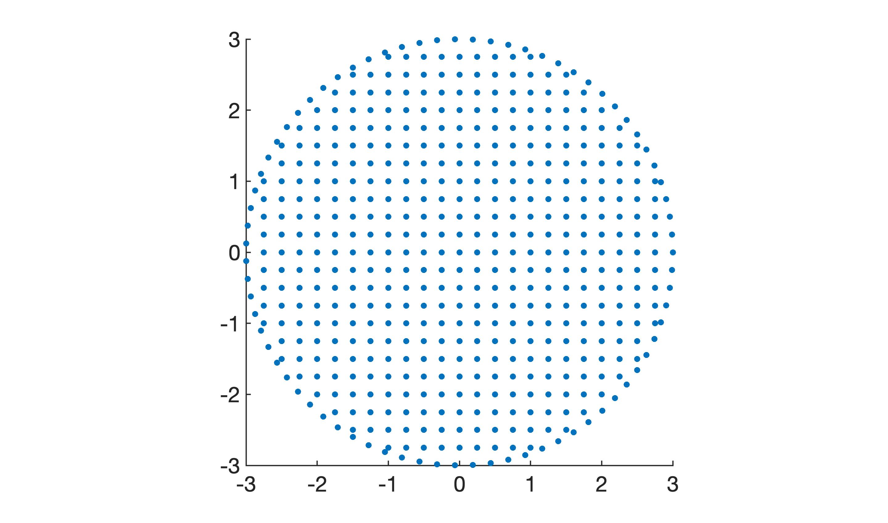
Figure 1. The domain $\Omega_{1}$ for $n_{x}=n_{y}=25,n_{b}=75,R=3$

We approximate the $x$ derivative at nodal points via $\bm{\mathsf{H}}^{-1}\bm{\mathsf{Q}}_{x}\bm{\mathsf{u}}\approx\frac{\partial u}{\partial x}$, where $\bm{\mathsf{H}}$ can be either $\bm{\mathsf{H}}_{\rm opt}$ or $\bm{\mathsf{H}}_{\rm unif}$. We follow an analogous procedure for the $y$ derivative. The $L_{2}$ error of the partial derivative of $u(x,y)$ with respect to $x$ can be approximated by:

$$\sqrt{(\bm{\mathsf{D}}_{x}\bm{\mathsf{u}}-\bm{\mathsf{u}}_{x})^{T}\bm{\mathsf{H}}(\bm{\mathsf{D}}_{x}\bm{\mathsf{u}}-\bm{\mathsf{u}}_{x})},$$ (3.21)

where $\bm{\mathsf{u}}_{x}$ is the vector containing point values of the exact derivative of $u$.

Tables 1 and 2 show the $L_{2}$ errors when computing $\frac{\partial u_{1}(x,y)}{\partial x}$ and $\frac{\partial u_{2}}{\partial x}$ using the SBP operators created under the two different norm matrices $\bm{\mathsf{H}}_{\rm opt},\bm{\mathsf{H}}_{\rm unif}$ on $\Omega_{1}$. The adjacency matrix $\bm{\mathsf{A}}$ (see Definition 1) is computed as follows: a point $(x_{j},y_{j})$ is a neighbor of a point $(x_{i},y_{i})$ if the distance between them is smaller than some distance. In these experiments, we use an arbitrary distance threshold of

$$r=2.5\frac{{\rm Diam}(\Omega_{1})}{\max(n_{x},n_{y})},$$

where ${\rm Diam}(\Omega_{1})$ is the diameter of the circular domain $\Omega_{1}$. We compare this method (which we refer to as the “Euclidean Radius” methods) with other methods of computing the adjacency matrix in Section 4.

Table 1 and 2 also show the computed convergence rates: $\text{log}_{2}\frac{error_{i-1}}{error_{i}}$. The operators are tested for the following grid sizes:

• Grid 1: $n_{x}=n_{y}=75,n_{b}=250$

• Grid 2: $n_{x}=n_{y}=150,n_{b}=500$

• Grid 3: $n_{x}=n_{y}=300,n_{b}=1000$

• Grid 4: $n_{x}=n_{y}=600,n_{b}=2000$

• Grid 5: $n_{x}=n_{y}=1200,n_{b}=4000$

Grid	$\frac{\partial u_{1}}{\partial x}$	Convergence Rate	$\frac{\partial u_{2}}{\partial x}$	Convergence Rate
$1$	$0.2605$		$0.06413$
$2$	$0.2013$	$0.3719$	$0.01626$	$1.980$
$3$	$0.1439$	$0.4842$	$0.004061$	$2.001$
$4$	$0.1072$	$0.4248$	$0.001205$	$1.753$
$5$	$0.07634$	$0.4896$	$0.0002794$	$2.109$

Table 1. $L_{2}$ error for $\frac{\partial u_{1}}{\partial x}|\frac{\partial u_{2}}{\partial x}$ using $\bm{\mathsf{H}}_{\rm opt}$ on $\Omega_{1}$.

Grid	$\frac{\partial u_{1}}{\partial x}$	Convergence Rate	$\frac{\partial u_{2}}{\partial x}$	Convergence Rate
$1$	$0.6704$		$0.02969$
$2$	$0.4763$	$0.4932$	$0.02008$	$0.5642$
$3$	$0.3328$	$0.5712$	$0.01286$	$0.6429$
$4$	$0.2389$	$0.4782$	$0.007390$	$0.7992$
$5$	$0.1690$	$0.4994$	$0.003894$	$0.9243$

Table 2. $L_{2}$ error for $\frac{\partial u_{1}}{\partial x}|\frac{\partial u_{2}}{\partial x}$ using $\bm{\mathsf{H}}_{\rm unif}$ on $\Omega_{1}$.

From Tables 1 and 2, we observe that the errors are consistently larger when using $\bm{\mathsf{H}}_{\rm unif}$. This suggests that using an optimized norm matrix $\bm{\mathsf{H}}_{\rm opt}$ as discussed in Section 3.3 reduces the approximation error.

3.5   On the observed convergence rates

We notice that in Tables 1 and 2 that the convergence rates are significantly lower for $\frac{\partial u_{2}}{\partial x}$ when compared to $\frac{\partial u_{1}}{\partial x}$. In particular, when using $\bm{\mathsf{H}}_{\rm opt}$, the convergence rate for $\frac{\partial u_{1}}{\partial x}$ is around $\frac{1}{2}$ while it is around 2 for $\frac{\partial u_{2}}{\partial x}$. This section will present numerical experiments which suggest that this difference in observed convergence rates is due to accuracy of the interior vs boundary stencils.

As we can see from Figure 2, the approximation error $\left|\bm{\mathsf{D}}_{x}\bm{\mathsf{u}}-\bm{\mathsf{u}}_{x}\right|$ is larger near the boundaries. However, since $\frac{\partial u_{2}}{\partial x}$ is close to $0$ at the boundary $\partial\Omega_{1}$, the errors near the boundaries are smaller for $u_{2}$. This is not the case for $u_{1}$.

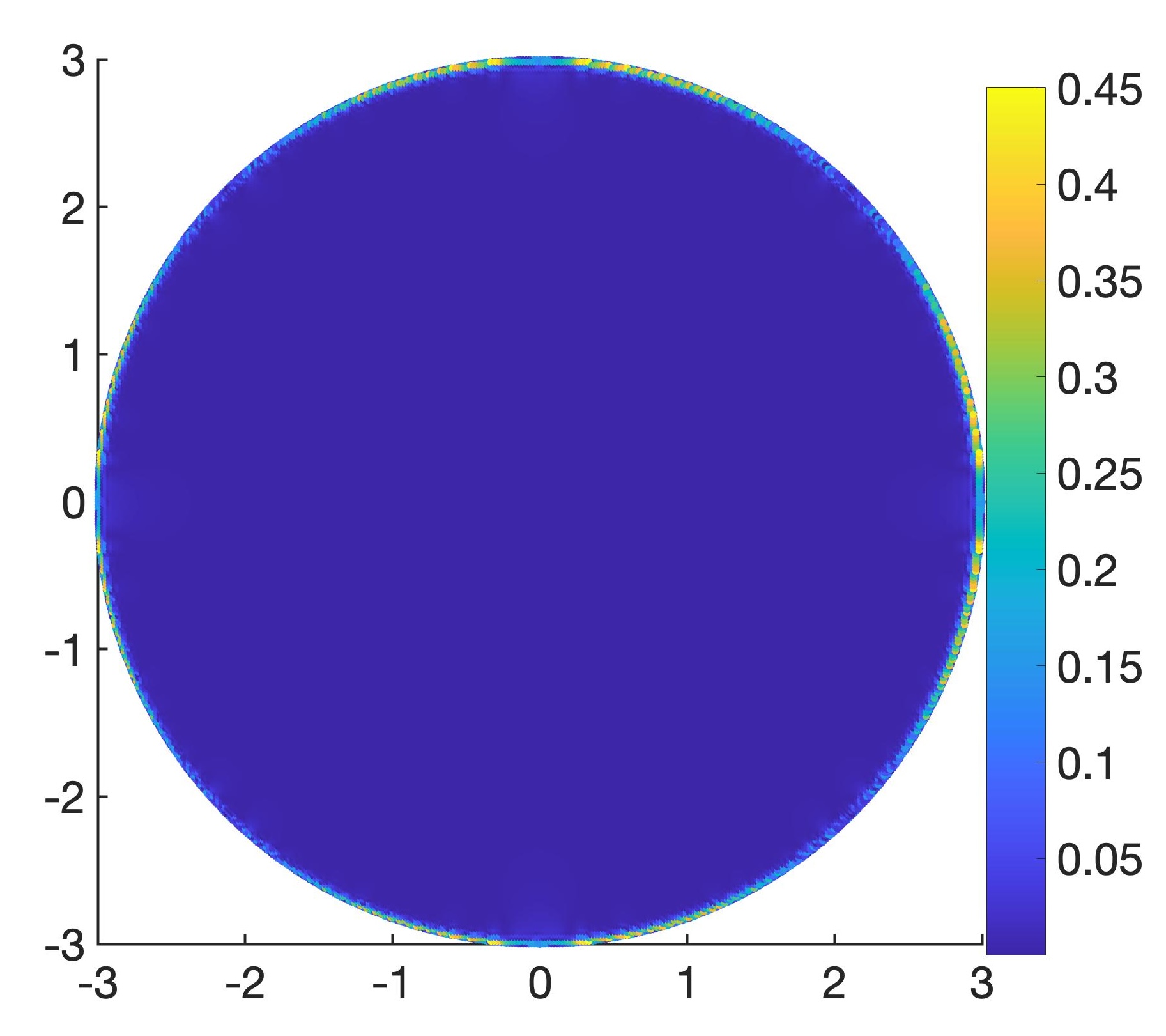
(a) $|\bm{\mathsf{D}}_{x}\bm{\mathsf{u_{1}}}-\bm{\mathsf{u}}_{\bm{\mathsf{1}}x}|$

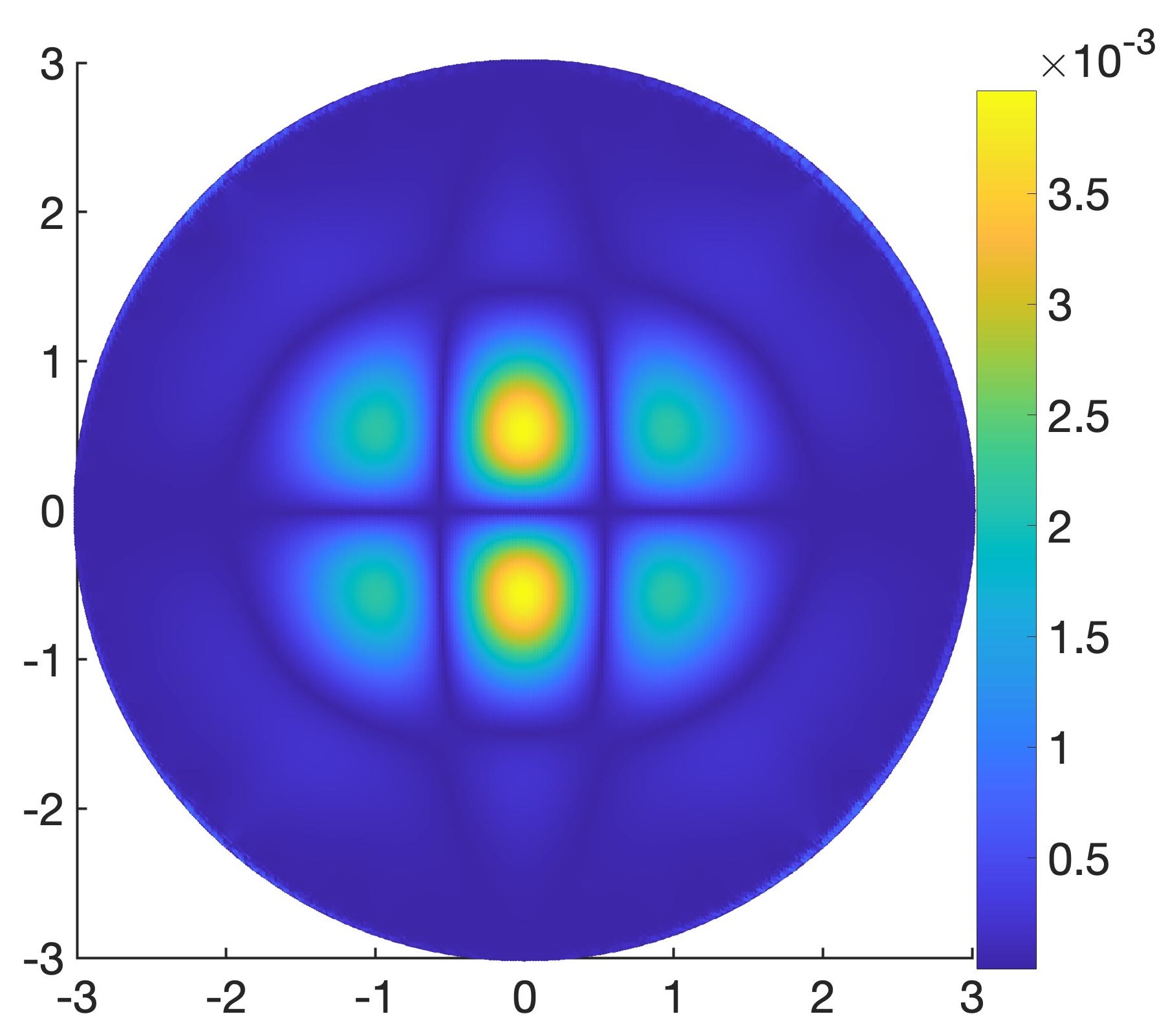
(b) $|\bm{\mathsf{D}}_{x}\bm{\mathsf{u_{2}}}-\bm{\mathsf{u}}_{\bm{\mathsf{2}}x}|$

Figure 2. Absolute values of the computed errors for the differential operators on $u_{1}$ and $u_{2}$ on Grid 3 using the “Euclidean Radius” adjacency method.

To further support the analysis from above, we perform the same numerical experiment of approximating $\frac{\partial u_{1}}{\partial x}$ and $\frac{\partial u_{2}}{\partial x}$, but this time on $\Omega_{2}$, which is a circle with three smaller circles cut out of the interior:

$$C_{i}:=\{(x,y)\in\mathbb{R}^{2}\;|\;(x-h_{i})^{2}+(y-k_{i})^{2}\leq s_{i}\}$$

$$\Omega_{2}:=\{(x,y)\in\mathbb{R}^{2}\;|\;x^{2}+y^{2}\leq R^{2},\;\;(x,y)\notin C_{i},\;\;\forall i\in\{1,2,..,m\}\}.$$

We set $R=3$, $s_{i}=\frac{2}{3}$, $h_{i}=\frac{3}{2}\cos\left(\frac{2\pi}{3}i\right)$, and $k_{i}=\frac{3}{2}\sin\left(\frac{2\pi}{3}i\right)$, for $i\in\{1,2,3\}$. By picking such a $\Omega_{2}$, $\frac{\partial u_{2}}{\partial x}$ is not approximately zero near the inner boundaries (ie: $\partial C_{i}$). Figure 3 shows $\Omega_{2}$ as reference.

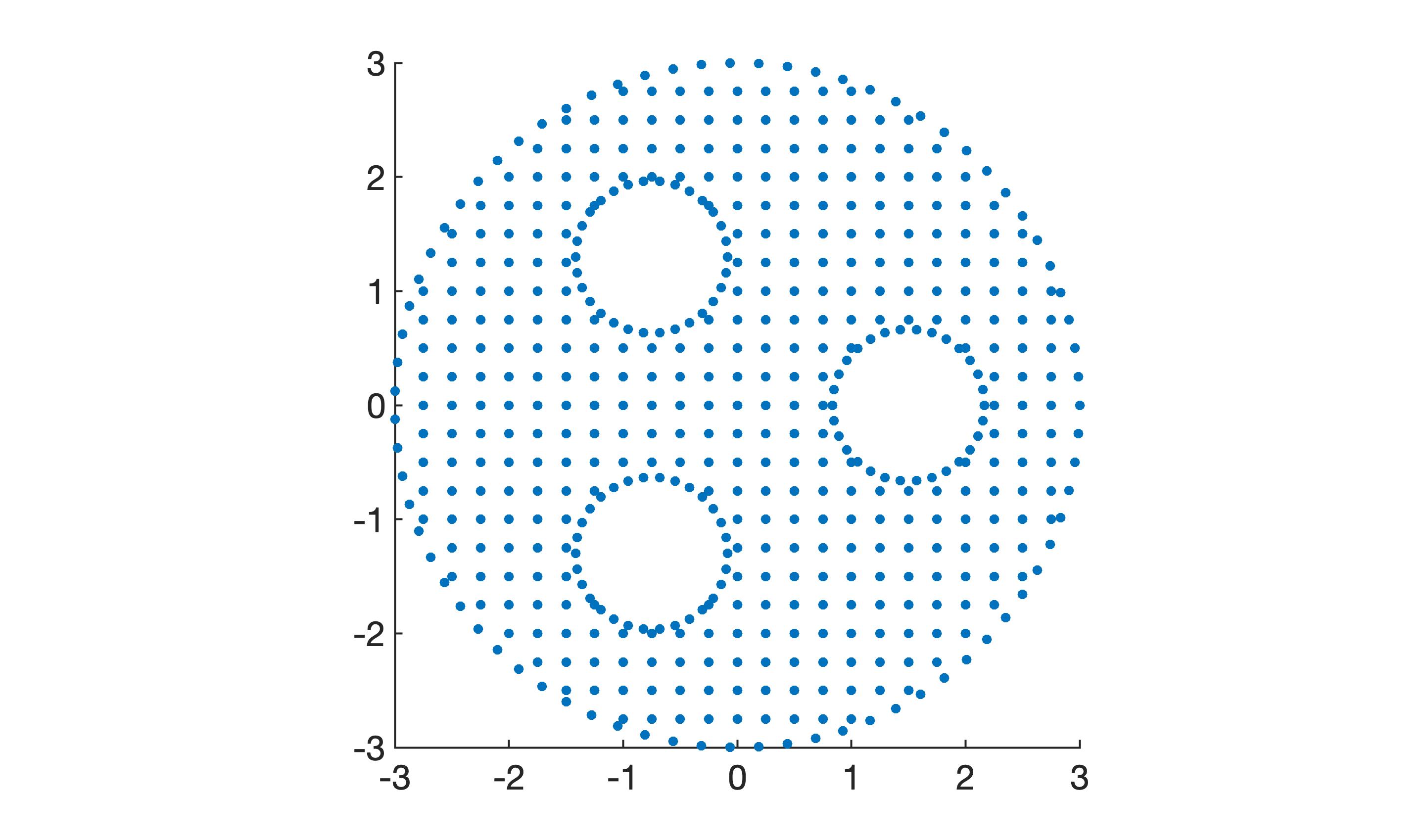
Figure 3. The domain $\Omega_{2}$ for $n_{x}=n_{y}=25,n_{b}=75,n_{i}=30,R=3$. Here, $n_{i}$ denotes the number of nodes on the boundary of each inner circle.

Table 3 displays the $L_{2}$ errors of $\frac{\partial u}{\partial x}$ on $\Omega_{2}$. Because $\frac{\partial u_{2}}{\partial x}$ is not near 0 near the inner boundaries of $\Omega_{2}$, we expect the convergence rates for both $\frac{\partial u_{2}}{\partial x}$ and $\frac{\partial u_{1}(x,y)}{\partial x}$ to both be around $\frac{1}{2}$. The grid sizes for $\Omega_{2}$ are as follows:

• Grid 1: $n_{x}=n_{y}=75,n_{b}=250,n_{i}=60$

• Grid 2: $n_{x}=n_{y}=150,n_{b}=500,n_{i}=120$

• Grid 3: $n_{x}=n_{y}=300,n_{b}=1000,n_{i}=240$

• Grid 4: $n_{x}=n_{y}=600,n_{b}=2000,n_{i}=480$

• Grid 5: $n_{x}=n_{y}=1200,n_{b}=4000,n_{i}=960$

where $n_{i}$ denotes the number of equispaced quadrature points placed on the boundary of $C_{i}$.

Table 3 show that the convergence rates are now similar for both $\frac{\partial u_{1}(x,y)}{\partial x}$ and $\frac{\partial u_{2}}{\partial x}$ at a rate of $\frac{1}{2}$. This is consistent with our expectation that the convergence rates should be similar for functions in which their values and their derivatives are not near 0 at the boundaries. From Figure 4, we see that the error is again greatest near the boundaries.

We further verify the observation made above about the worse behavior near the boundaries. We check the $L_{\infty}$ error of $\frac{\partial u_{1}}{\partial x}$ on $\Omega_{1}$ but this time differentiate between the nodes near the boundary: $\{(x,y)\in S|x^{2}+y^{2}\geq 4\}$ and nodes far from the boundary $\{(x,y)\in S|x^{2}+y^{2}<4\}$. We use the $L_{\infty}$ error instead of the $L_{2}$ error to avoid needing to define appropriate quadratures over subsets of points. Table 4 shows the results and convergence rates.

Grid	$\frac{\partial u_{1}}{\partial x}$	Convergence Rate	$\frac{\partial u_{2}}{\partial x}$	Convergence Rate
$1$	$0.3547$		$0.1622$
$2$	$0.2695$	$0.3963$	$0.1000$	$0.6978$
$3$	$0.1973$	$0.4499$	$0.07470$	$0.4208$
$4$	$0.1440$	$0.4543$	$0.05211$	$0.5195$
$5$	$0.1018$	$0.5003$	$0.03841$	$0.4400$

Table 3. $L_{2}$ errors and computed convergence rates for $\frac{\partial u_{1}}{\partial x}$ and $\frac{\partial u_{2}}{\partial x}$ on $\Omega_{2}$.

Grid	$x^{2}+y^{2}>4$	Convergence Rate	$x^{2}+y^{2}\leq 4$	Convergence Rate
$1$	$0.4213$		$0.005472$
$2$	$0.4819$	$-0.1938$	$0.002672$	$1.0342$
$3$	$0.4505$	$0.09721$	$7.631\times 10^{-4}$	$1.8081$
$4$	$0.4767$	$-0.08155$	$3.250\times 10^{-4}$	$1.2312$
$5$	$0.5122$	$-0.1036$	$9.399\times 10^{-5}$	$1.7901$

Table 4. $L_{\infty}$ error for $\frac{\partial u_{1}}{\partial x}$ at interior vs exterior nodes.

From Table 4, we do indeed see that the error is much more significant (a few order of magnitudes) larger near the boundaries. Furthermore, combined with our observations from Table 1 and 3, it also suggests (though would need to be proven) that for sufficiently close nodes to the boundaries, the convergence rate is 0.5 and the convergence rate for nodes sufficiently far from the boundary nodes achieve between first and second order accuracy. This suggests that the meshfree interior stencils are second order accurate, while the boundary stencils are inconsistent in the sense that the pointwise error does not converge to zero as the mesh size decreases. However, experiments in Section 6 suggest that numerical approximations of solutions of PDEs achieve first order accuracy in the $L^{2}$ norm. It is possible that the meshfree operators constructed here are first order accurate in some sense, but not in a pointwise sense. Analyzing this will be the focus of future work.

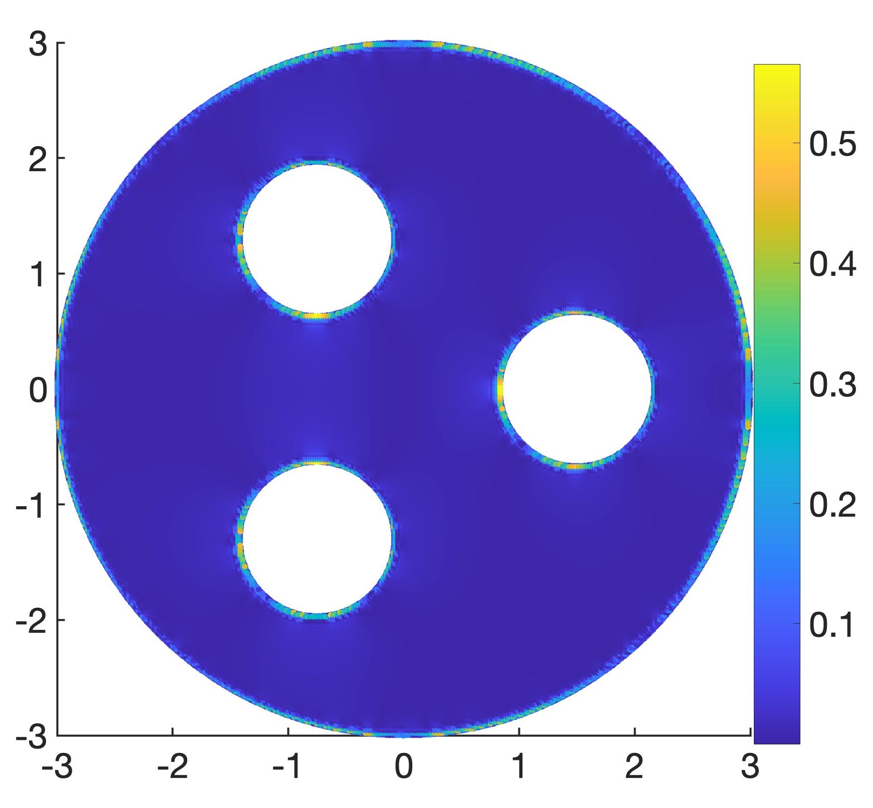
(a) $|\bm{\mathsf{D}}_{x}\bm{\mathsf{u_{1}}}-\bm{\mathsf{u}}_{\bm{\mathsf{1}}x}|$

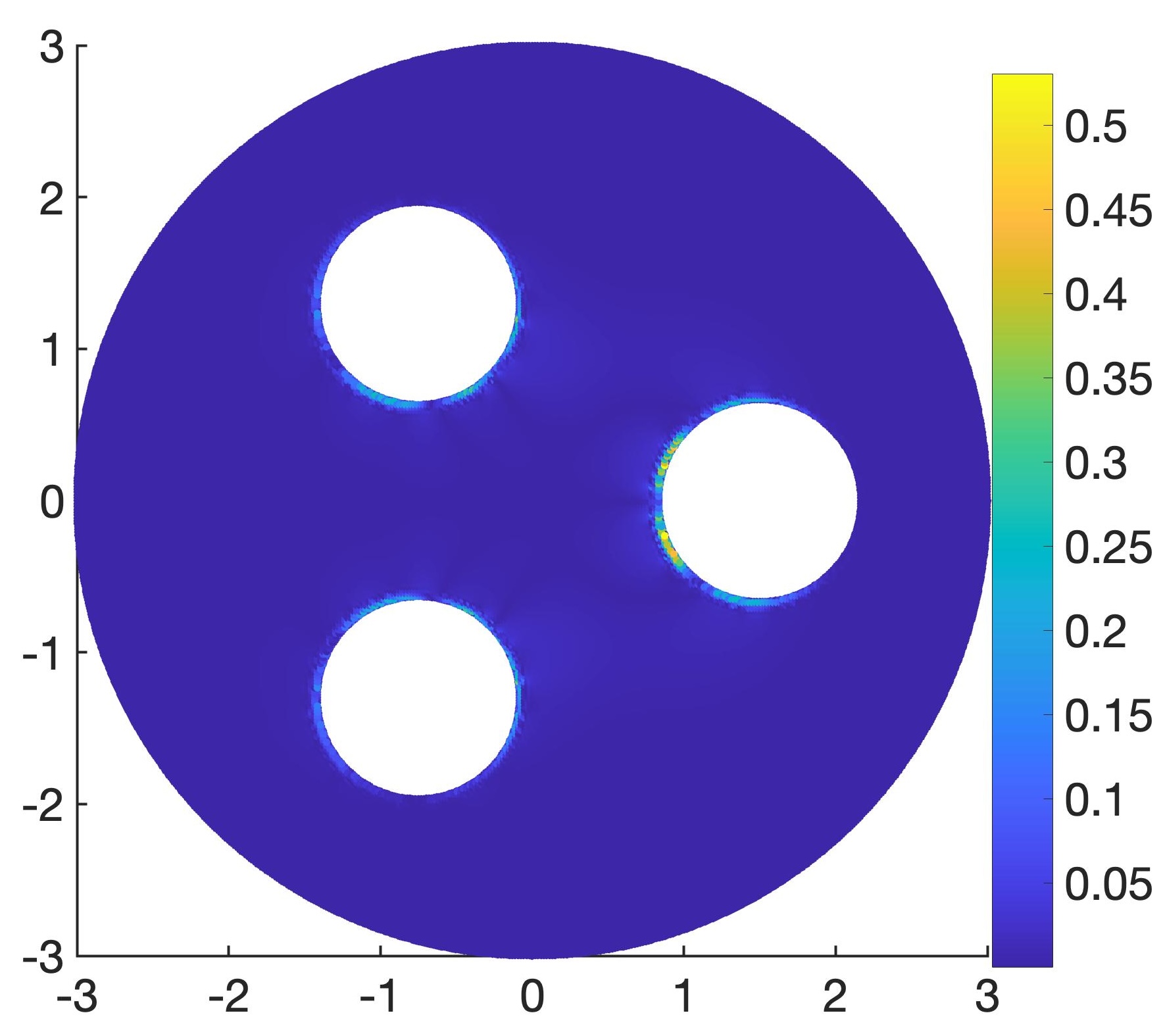
(b) $|\bm{\mathsf{D}}_{x}\bm{\mathsf{u_{2}}}-\bm{\mathsf{u}}_{\bm{\mathsf{2}}x}|$

Figure 4. Absolute value errors for differential operators on $u_{1}$ and $u_{2}$ on $\Omega_{2}$ (Euclidean Radius, Grid 3).

4   Finding Suitable Notion of Adjacency

An important detail of the construction that was skipped over in previous sections is the construction of the adjacency/connectivity matrix $\bm{\mathsf{A}}$. In this section, we will explore several notions of connectivity through numerical experiments and determine which produces meshfree operators which result in lower errors. We will also discuss a few implementation details. While the only requirement on the adjacency matrix $\bm{\mathsf{A}}$ is that it represents a fully connected graph between the nodes, it is important to make sure that the notion of connectivity defined maintains sparsity but does not decrease accuracy.

Let $v_{i}$ be the node corresponding to $(x_{i},y_{i})\in S$ and let $d(v_{i},v_{j})$ correspond to the Euclidean distance between $v_{i}$ and $v_{j}$. We explore the following four notions of connectivity:

1. Euclidean Radius: we say that $v_{i}$ and $v_{j}$ are adjacent if $d(v_{i},v_{j})\leq r$. Section 4.1 gives further details on the efficient implementation.

2. Minimum spanning tree: Using the nodes $v_{1},...,v_{N}$ and $d(v_{i},v_{j})$, we can form the adjacency matrix from a minimum spanning tree (the graph with the minimum number of edges such that there is a path between every pair of nodes).

3. Degree 1 Delaunay: We call $v_{i}$ and $v_{j}$ adjacent if they are neighbors in a Delaunay triangulation on $S$.

4. Degree 2 Delaunay: We call $v_{i}$ and $v_{j}$ adjacent if they are neighbors in a Delaunay triangulation on $S$ or if $v_{i}$ and $v_{j}$ share a common neighbor.

Remark 1.

We note that the Delaunay triangulation connectivity methods are not “meshfree”. However, unlike mesh-based finite element methods, the quality and regularity of the mesh generated by Delaunay triangulation does not significantly impact solution quality [37]. Moreover, we consider Delaunay triangulations only as a comparison against truly meshfree notions of adjacency, such as the Euclidean Radius.

Grid	Euclidean Radius		Delaunay Deg 1		Delaunay Deg 2
	Error	Rate	Error	Rate	Error	Rate
$1$	$0.2605$		$0.2909$		$0.2103$
$2$	$0.2013$	$0.3719$	$0.2246$	$0.3732$	$0.1656$	$0.3447$
$3$	$0.1439$	$0.4248$	$0.1573$	$0.5318$	$0.1134$	$0.5463$
$4$	$0.1072$	$0.4248$	$0.1163$	$0.4357$	$0.0853$	$0.4108$
$5$	$0.07635$	$0.4896$	$0.08369$	$0.4747$	$0.0607$	$0.4908$

Table 5. $L_{2}$ error for $\frac{\partial u_{1}}{\partial x}$ and computed convergence rates on $\Omega_{1}$.

Grid	Euclidean Radius		Delaunay Deg 1		Delaunay Deg 2
	Error	Rate	Error	Rate	Error	Rate
$1$	$0.06413$		$0.03321$		$0.0700$
$2$	$0.01626$	$1.980$	$0.01591$	$1.062$	$0.0197$	$1.829$
$3$	$0.004061$	$2.001$	$0.008208$	$0.9548$	$0.00753$	$1.387$
$4$	$0.001205$	$1.753$	$0.004118$	$0.9951$	$0.003561$	$1.080$
$5$	$0.0002794$	$2.109$	$0.002072$	$0.9909$	$0.001787$	$0.9947$

Table 6. $L_{2}$ error for $\frac{\partial u_{2}}{\partial x}$ and computed convergence rates on $\Omega_{1}$.

We test the accuracy of the differentiation matrices created by the four different notions of adjacency by approximating $\frac{\partial u_{1}}{\partial x}$, $\frac{\partial u_{2}}{\partial x}$. Tables 5 and 6 display the $\frac{\partial u_{1}}{\partial x}$, $\frac{\partial u_{2}}{\partial x}$ $L_{2}$ errors when approximated by the SBP operators with the various adjacency methods on $\Omega_{1}$ ($R=3$).

All Euclidean Radius methods used $r=2.5\frac{6}{n_{x}}$, which we chose heuristically to balance accuracy and sparsity of the resulting differentiation operators. Additionally, while we do not show them, the $L_{2}$ errors for $\frac{\partial u_{1}}{\partial x}$, $\frac{\partial u_{1}}{\partial y}$, $\frac{\partial u_{2}}{\partial x}$, and $\frac{\partial u_{2}}{\partial y}$ are very similar to the errors for $\frac{\partial u_{1}}{\partial x}$ and $\frac{\partial u_{2}}{\partial x}$, which are shown in Tables 7 and 8.

We make a couple of observations. The first observation is that determining the adjacency matrix using a minimum spanning tree fails to produce accurate meshfree operators. We do not display the results in Table 5 and Table 6 because the error blows up as the number of points increases. The second observation is that determining the adjacency matrix using the Delaunay degree 1 method results in a larger error than the determining the adjacency matrix using the Delaunay degree 2 method. Both Delaunay degree 2 and Euclidean radius methods result in similar errors for this test case and show similar convergence behavior.

When computing $\frac{\partial u_{1}}{\partial x}$, the rate of convergence of the error is approximately $0.5$, while the rate of convergence of the error when computing $\frac{\partial u_{2}}{\partial x}$ is around $2$ for the Euclidean Radius method and $1$ for the Delaunay degree 2 method. Note that, since $\frac{\partial u_{2}}{\partial x}\approx 0$ near the boundaries (as discussed in Section 3.5), this effectively tests only accuracy of the interior stencil. These results suggest that interior stencils constructed using the Euclidean Radius approach are second order accurate, while interior stencils constructed using the Delaunay degree 2 approach are only first order accurate.

To differentiate between the Euclidean Radius and Delaunay Degree 2 notion of adjacency, we perform the same numerical experiment but this time on $\Omega_{2}$. Tables 7 and 8 display the $L_{2}$ errors for the Euclidean Radius and Delaunay Degree 2 methods on $\Omega_{2}$.

Grid	Euclidean Radius		Delaunay Deg 2
$1$	$0.3547$		$0.3925,$
$2$	$0.2695$	$0.3963$	$0.2757$	$0.5096$
$3$	$0.1973$	$0.4499$	$0.1968$	$0.4864$
$4$	$0.1440$	$0.4543$	$0.1404$	$0.4872$
$5$	$0.1018$	$0.5003$	$0.1297$	$0.1144$

Table 7. $L_{2}$ error for $\frac{\partial u_{1}}{\partial x}$ on domain $\Omega_{2}$.

Grid	Euclidean Radius		Delaunay Deg 2
$1$	$0.1622$		$0.1818$
$2$	$0.1000$	$0.6978$	$0.1259$	$0.5301$
$3$	$0.07470$	$0.4208$	$0.09318$	$0.4342$
$4$	$0.05211$	$0.5195$	$0.06450$	$0.5307$
$5$	$0.03841$	$0.4400$	$0.07840$	$-0.2816$

Table 8. $L_{2}$ error for $\frac{\partial u_{2}}{\partial x}$ on domain $\Omega_{2}$.

From Tables 7 and 8, we see that the Euclidean Radius and Delaunay degree 2 method both gives similar errors and convergence rates for the first four grid sizes. However, for the densest grid, the Euclidean Radius continues to converge at a rate of $\frac{1}{2}$ while the errors for the Delaunay degree 2 method essentially plateau. Hence, all numerical results presented later in this paper will use the Euclidean Radius notion of adjacency to build meshfree SBP differentiation operators.

4.1   Details on the computational implementation

For large sets of points in $S$, care must be taken to construct the SBP matrices in an efficient manner. For example, from Table 5 and 6, there are $1132984$ points in $S$ for the $n_{x}=n_{y}=1200,n_{b}=4000$ case (Grid 5). Hence $\bm{\mathsf{Q}}_{x},\bm{\mathsf{Q}}_{y},\bm{\mathsf{E}}_{x},\bm{\mathsf{E}}_{y},\bm{\mathsf{S}}_{x},\bm{\mathsf{S}}_{y},\bm{\mathsf{L}}$, and $\bm{\mathsf{D}}_{x},\bm{\mathsf{D}}_{y}$ are all $1132984$ by $1132984$ matrices. We discuss a few implementation details used in our numerical experiments. The full code can be found in the reproducibility repository In addition to using vectorized indexing and efficient native MATLAB matrix operations, we used the following additional steps to reduce the computational cost of computing SBP matrices:

1. All matrices were constructed in MATLAB using various built-in packages and functions. Sparse matrices were utilized to reduce memory and computational costs.

2. In order to effectively calculate $\bm{\mathsf{L}}$, we construct it given the adjacency matrix $\bm{\mathsf{A}}$. However, constructing $\bm{\mathsf{A}}$ using a naive implementation of the Euclidean Radius method (e.g., create a distance matrix using pdist in MATLAB) is infeasible for large point sets. Instead, we construct the adjacency matrix using the Euclidean distance K-d tree implementation KDTreeSearcher in Matlab [14].

3. Because the Delaunay triangulation sometimes connects nodes across boundaries of the interior circles in $\Omega_{2}$, the resulting errors are very large at the boundaries. We ensure this does not happen for the Delaunay Degree 2 triangulation method by manually removing connections between nodes situated across interior circle boundaries.

4. As mentioned in section 3.4, before solving (3.20) is computationally expensive for large point sets. We use a splitting conic solver to reduce the computational cost of solving (3.20) [22].

Table 9 shows the computational runtimes of several steps involved in generating the SBP differentiation operators for the $n_{x}=n_{y}=1200,n_{b}=4000$ case. Notice that the majority of the time was spent constructing $\bm{\mathsf{\Psi}}_{x}$ and $\bm{\mathsf{\Psi}}_{y}$. This was because a large $1132984$ by $1132984$ matrix system is solved in equation 3.16. This can be potentially sped up with a more efficient numerical method (we utilize the default solver implemented in MATLAB’s “backslash”). For example, one can invert L efficiently using an algebraic multigrid solver [33].

Table 9. Time taken for each matrix generation of the SBP matrices (seconds)

$\bm{\mathsf{A}}$	$\bm{\mathsf{L}}$	$\bm{\mathsf{E}}_{x},\bm{\mathsf{E}}_{y}$	$\bm{\mathsf{\bm{\mathsf{\Psi}}}}_{x},\bm{\mathsf{\bm{\mathsf{\Psi}}}}_{y}$	$\bm{\mathsf{S}}_{x},\bm{\mathsf{S}}_{y}$	$\bm{\mathsf{Q}}_{x},\bm{\mathsf{Q}}_{y}$	$\bm{\mathsf{H}}_{\rm opt}$	Total Time
$5.0217$	$0.9286$	$0.0128$	$163.9192$	$8.8232$	$0.3200$	$5.5201$	$189.5627$

5   A robust first order accurate meshfree method

In this section, we apply our meshfree SBP operators to the numerical solution of systems of nonlinear conservation laws:

$$\frac{\partial\bm{u}}{\partial t}+\frac{\partial\bm{f}_{x}(\bm{u})}{\partial x}+\frac{\partial\bm{f}_{y}(\bm{u})}{\partial y}=\bm{0},$$

$$\bm{u}(x,y)=\bm{f}_{bc}(x,y),\quad\forall(x,y)\in M\cap S$$

Here, $\bm{u}\in[L^{2}(\Omega)]^{n}$, $\bm{f}_{x},\bm{f}_{y},\bm{f}_{bc}\in[C^{0}(\mathbb{R}^{n})]^{n}$, and $M$ is an appropriate subset of $\partial\Omega$ on which we enforce boundary conditions.

5.1   Notation

To begin, we introduce some notation. Recall the notation used in (5), where $\bm{u}\in[L^{2}(\Omega)]^{n}$ denotes the solution we are trying to approximate, where $\bm{u}=[u^{1},u^{2},...\,,u^{n}]$. Here, $u^{i}$ denotes individual components of the solution, where $u^{1},...\,,u^{n}\in L^{2}(\Omega)$. We denote the numerical approximation of point values of $\bm{u}$ evaluated on $(x_{i},y_{i})\in S$ as:

$$\accentset{\rightharpoonup}{\bm{\mathsf{u}}}=\begin{pmatrix}[u^{1}(x_{1},y_{1})\,,...\,,u^{n}(x_{1},y_{1})]\\[10.00002pt] [u^{1}(x_{2},y_{2})\,,...\,,u^{n}(x_{2},y_{2})]\\[10.00002pt] \vdots\\[5.0pt] [u^{1}(x_{N},y_{N})\,,...\,,u^{n}(x_{N},y_{N})]\end{pmatrix}$$ (5.1)

We denote $\accentset{\rightharpoonup}{\bm{\mathsf{u}}}_{i}$ as the $i^{th}$ entry of $\accentset{\rightharpoonup}{\bm{\mathsf{u}}}$. Hence $\accentset{\rightharpoonup}{\bm{\mathsf{u}}}_{i}=[u^{1}(x_{i},y_{i})\,,...\,,u^{n}(x_{i},y_{i})]$. Recall again from (5) that $\bm{f}_{x}:\mathbb{R}^{n}\rightarrow\mathbb{R}^{n}$, where $\bm{f}_{x}=[f_{x}^{1},f_{x}^{2}\,,...\,,f_{x}^{n}]$ and $f_{x}^{1}\,,...\,,f_{x}^{n}\in C^{0}(\mathbb{R}^{n})$.

We now define the behavior of $\bm{f}_{x}(\accentset{\rightharpoonup}{\bm{\mathsf{u}}})$ (e.g., $\bm{f}_{x}(\bm{u})$ evaluated over $S$) as:

$$\bm{f_{x}}(\accentset{\rightharpoonup}{\bm{\mathsf{u}}})=\begin{pmatrix}\bm{f}_{x}(\accentset{\rightharpoonup}{\bm{\mathsf{u}}}_{1})\\[10.00002pt] \bm{f}_{x}(\accentset{\rightharpoonup}{\bm{\mathsf{u}}}_{2})\\[10.00002pt] \vdots\\[5.0pt] \bm{f}_{x}(\accentset{\rightharpoonup}{\bm{\mathsf{u}}}_{N})\\ \end{pmatrix}=\begin{pmatrix}[f_{x}^{1}(\accentset{\rightharpoonup}{\bm{\mathsf{u}}}_{1})\,,...\,,f_{x}^{n}(\accentset{\rightharpoonup}{\bm{\mathsf{u}}}_{1})]\\[10.00002pt] [f_{x}^{1}(\accentset{\rightharpoonup}{\bm{\mathsf{u}}}_{2})\,,...\,,f_{x}^{n}(\accentset{\rightharpoonup}{\bm{\mathsf{u}}}_{2})]\\[10.00002pt] \vdots\\[5.0pt] [f_{x}^{1}(\accentset{\rightharpoonup}{\bm{\mathsf{u}}}_{N})\,,...\,,f_{x}^{n}(\accentset{\rightharpoonup}{\bm{\mathsf{u}}}_{N})]\\[10.00002pt] \end{pmatrix}$$ (5.2)

Furthermore, consider the matrix-vector multiplication $\bm{\mathsf{D}}_{x}\bm{f}_{x}(\accentset{\rightharpoonup}{\bm{\mathsf{u}}})$. We define this behavior as follows:

$$\bm{\mathsf{D}}_{x}\bm{f}_{x}(\accentset{\rightharpoonup}{\bm{\mathsf{u}}})=\begin{pmatrix}\sum_{i=1}^{N}(\bm{\mathsf{D}}_{x})_{1i}\bm{f}_{x}(\accentset{\rightharpoonup}{\bm{\mathsf{u}}}_{i})\\[10.00002pt] \sum_{i=1}^{N}(\bm{\mathsf{D}}_{x})_{2i}\bm{f}_{x}(\accentset{\rightharpoonup}{\bm{\mathsf{u}}}_{i})\\[10.00002pt] \vphantom{\bm{\mathsf{D}}_{x}}\vdots\\[5.0pt] \sum_{i=1}^{N}(\bm{\mathsf{D}}_{x})_{Ni}\bm{f}_{x}(\accentset{\rightharpoonup}{\bm{\mathsf{u}}}_{i})\\[10.00002pt] \end{pmatrix}=\begin{pmatrix}\sum_{i=1}^{N}(\bm{\mathsf{D}}_{x})_{1i}[f_{x}^{1}(\accentset{\rightharpoonup}{\bm{\mathsf{u}}}_{i})\,,...\,,f_{x}^{n}(\accentset{\rightharpoonup}{\bm{\mathsf{u}}}_{i})]\\[10.00002pt] \sum_{i=1}^{N}(\bm{\mathsf{D}}_{x})_{2i}[f_{x}^{1}(\accentset{\rightharpoonup}{\bm{\mathsf{u}}}_{i})\,,...\,,f_{x}^{n}(\accentset{\rightharpoonup}{\bm{\mathsf{u}}}_{i})]\\[10.00002pt] \vdots\\[5.0pt] \sum_{i=1}^{N}(\bm{\mathsf{D}}_{x})_{Ni}[f_{x}^{1}(\accentset{\rightharpoonup}{\bm{\mathsf{u}}}_{i})\,,...\,,f_{x}^{n}(\accentset{\rightharpoonup}{\bm{\mathsf{u}}}_{i})]\\[10.00002pt] \end{pmatrix}$$ (5.3)

5.2   Discretization

Inserting our meshfree SBP differentiation operators into (5) yields:

$$\bm{\mathsf{\accentset{\rightharpoonup}{u}}}_{t}+\bm{\mathsf{D}}_{x}\bm{\mathsf{f}}_{x}(\bm{\mathsf{\accentset{\rightharpoonup}{u}}})+\bm{\mathsf{D}}_{y}\bm{\mathsf{f}}_{y}(\bm{\mathsf{\accentset{\rightharpoonup}{u}}})=\bm{0}$$ (5.4)

Multiplying $\bm{\mathsf{H}}$ to both sides yields:

$$\bm{\mathsf{H}}\bm{\mathsf{\accentset{\rightharpoonup}{u}}}_{t}+\bm{\mathsf{Q}}_{x}\bm{\mathsf{f}}_{x}(\bm{\mathsf{\accentset{\rightharpoonup}{u}}})+\bm{\mathsf{Q}}_{y}\bm{\mathsf{f}}_{y}(\bm{\mathsf{\accentset{\rightharpoonup}{u}}})=0$$ (5.5)

Using (2.9), we have that

$$\bm{\mathsf{Q}}_{x}\bm{\mathsf{f}}_{x}(\bm{\mathsf{\accentset{\rightharpoonup}{u}}})=\bm{\mathsf{E}}_{x}\bm{\mathsf{f}}_{x}(\bm{\mathsf{\accentset{\rightharpoonup}{u}}})-\bm{\mathsf{Q}}_{x}^{T}\bm{\mathsf{f}}_{x}(\bm{\mathsf{\accentset{\rightharpoonup}{u}}}).$$ (5.6)

We make the observation that the term $\bm{\mathsf{E}}_{x}\bm{\mathsf{f}}_{x}(\bm{\mathsf{\accentset{\rightharpoonup}{u}}})$ only depends on the points in $S\cap\partial\Omega$. Therefore we make the substitution $\accentset{\rightharpoonup}{\bm{\mathsf{u}}}$ with $\accentset{\rightharpoonup}{\bm{\mathsf{u}}}_{BC}$ where:

$$\forall(x_{i},y_{i})\in S:(\accentset{\rightharpoonup}{\bm{\mathsf{u}}}_{BC})_{i}=\left\{\begin{array}[]{lr}\bm{f}_{bc}(x_{i},y_{i})&\text{if $(x_{i},y_{i})\in M$}\\ \bm{\mathsf{u}}_{i}&\text{otherwise}\end{array}\right.$$ (5.7)

This allows us to weakly enforce the boundary conditions by replacing the right hand side of (5.6) by the following

$$\bm{\mathsf{E}}_{x}\bm{\mathsf{f}}_{x}(\bm{\mathsf{u}}_{BC})-\bm{\mathsf{Q}}_{x}^{T}\bm{\mathsf{f}}_{x}(\bm{\mathsf{u}}).$$ (5.8)

Using the SBP property (2.9) again yields:

$$\bm{\mathsf{E}}_{x}\bm{\mathsf{f}}_{x}(\accentset{\rightharpoonup}{\bm{\mathsf{u}}}_{BC})-\bm{\mathsf{Q}}_{x}^{T}\bm{\mathsf{f}}_{x}(\accentset{\rightharpoonup}{\bm{\mathsf{u}}})=\bm{\mathsf{Q}}_{x}\bm{\mathsf{f}}_{x}(\accentset{\rightharpoonup}{\bm{\mathsf{u}}})+\bm{\mathsf{E}}_{x}({\bm{\mathsf{f}}_{x}(\accentset{\rightharpoonup}{\bm{\mathsf{u}}}_{BC})-\bm{\mathsf{f}}_{x}(\accentset{\rightharpoonup}{\bm{\mathsf{u}}})})$$ (5.9)

Together, this results in an algebraic formulation with weakly imposed boundary conditions:

$$\bm{\mathsf{H}}\accentset{\rightharpoonup}{\bm{\mathsf{u}}}_{t}+\bm{\mathsf{Q}}_{x}\bm{\mathsf{f}}_{x}(\accentset{\rightharpoonup}{\bm{\mathsf{u}}})+\bm{\mathsf{Q}}_{y}\bm{\mathsf{f}}_{y}(\accentset{\rightharpoonup}{\bm{\mathsf{u}}})+\bm{\mathsf{E}}_{x}({\bm{\mathsf{f}}_{x}(\accentset{\rightharpoonup}{\bm{\mathsf{u}}}_{BC})-\bm{\mathsf{f}}_{x}(\accentset{\rightharpoonup}{\bm{\mathsf{u}}})})+\bm{\mathsf{E}}_{y}({\bm{\mathsf{f}}_{y}(\accentset{\rightharpoonup}{\bm{\mathsf{u}}})-\bm{\mathsf{f}}_{y}(\accentset{\rightharpoonup}{\bm{\mathsf{u}}})})=\bm{0}$$ (5.10)

5.3   Stabilization

The formulation (5.10) corresponds to a non-dissipative “central” scheme. However, for solutions of nonlinear conservation laws with sharp gradients, shocks, or other under-resolved solution features, non-dissipative schemes can result in spurious oscillations [19, 18]. To avoid this, we add upwinding-like dissipation using an approach similar to techniques used in [5].

Denote $\bm{r}_{i}$ as the $i^{\text{th}}$ entry of $\bm{\mathsf{Q}}_{x}\bm{\mathsf{f}}_{x}(\accentset{\rightharpoonup}{\bm{\mathsf{u}}})+\bm{\mathsf{Q}}_{y}\bm{\mathsf{f}}_{y}(\accentset{\rightharpoonup}{\bm{\mathsf{u}}})$. Then, we observe the following:

$$\bm{r}_{i} =\sum_{j}(\bm{\mathsf{Q}}_{x})_{ij}\bm{\mathsf{f}}_{x}(\accentset{\rightharpoonup}{\bm{\mathsf{u}}}_{j})+(\bm{\mathsf{Q}}_{y})_{ij}\bm{\mathsf{f}}_{y}(\accentset{\rightharpoonup}{\bm{\mathsf{u}}}_{j})$$ (5.11)

$$=2\sum_{j}(\bm{\mathsf{Q}}_{x})_{ij}\frac{(\bm{\mathsf{f}}_{x}(\accentset{\rightharpoonup}{\bm{\mathsf{u}}}_{j})+\bm{\mathsf{f}}_{x}(\accentset{\rightharpoonup}{\bm{\mathsf{u}}}_{i}))}{2}+(\bm{\mathsf{Q}}_{y})_{ij}\frac{(\bm{\mathsf{f}}_{y}(\accentset{\rightharpoonup}{\bm{\mathsf{u}}}_{j})+\bm{\mathsf{f}}_{y}(\accentset{\rightharpoonup}{\bm{\mathsf{u}}}_{i}))}{2}$$ (5.12)

Note that moving from (5.11) to (5.12) is valid because $\bm{\mathsf{Q_{x}}}\bm{1}=\bm{0}$ by the first order consistency condition, which implies that $\sum_{j}(\bm{\mathsf{Q}}_{x})_{ij}=0$. Because multiplying both sides by $\bm{\mathsf{f}}_{x}(\accentset{\rightharpoonup}{\bm{\mathsf{u}}}_{i})$ still yields $\bm{0}$, $\sum_{j}(\bm{\mathsf{Q}}_{x})_{ij}\bm{\mathsf{f}}_{x}(\accentset{\rightharpoonup}{\bm{\mathsf{u}}}_{i})=\sum_{j}(\bm{\mathsf{Q}}_{y})_{ij}\bm{\mathsf{f}}_{y}(\accentset{\rightharpoonup}{\bm{\mathsf{u}}}_{i})=\bm{0}$, implying that (5.12) is equivalent to (5.11).

We can rewrite (5.12) as

$$\bm{r}_{i}(\accentset{\rightharpoonup}{\bm{\mathsf{u}}})=2\sum_{j}\frac{1}{2}\left(\begin{bmatrix}\bm{\mathsf{f}}_{x}(\accentset{\rightharpoonup}{\bm{\mathsf{u}}}_{i})\\ \bm{\mathsf{f}}_{y}(\accentset{\rightharpoonup}{\bm{\mathsf{u}}}_{i})\end{bmatrix}+\begin{bmatrix}\bm{\mathsf{f}}_{x}(\accentset{\rightharpoonup}{\bm{\mathsf{u}}}_{j})\\ \bm{\mathsf{f}}_{y}(\accentset{\rightharpoonup}{\bm{\mathsf{u}}}_{j})\end{bmatrix}\right)\cdot\begin{bmatrix}(\bm{\mathsf{Q}}_{x})_{ij}\\ (\bm{\mathsf{Q}}_{y})_{ij}\end{bmatrix}$$ (5.13)

We make the observation that (5.13) is similar to a central flux, where $(\bm{\mathsf{Q}}_{x})_{ij},(\bm{\mathsf{Q}}_{y})_{ij}$ are playing the role of the “normal vector”. However, because the central flux is non-dissipative, we replace the central flux with the local Lax Friedrichs flux in our formulation as follows:

$$\bm{r}_{i}(\accentset{\rightharpoonup}{\bm{\mathsf{u}}})=2\sum_{j\in N(i)}\|\bm{n}_{ij}\|\frac{1}{2}\left(\begin{bmatrix}\bm{\mathsf{f}}_{x}(\accentset{\rightharpoonup}{\bm{\mathsf{u}}}_{i})\\ \bm{\mathsf{f}}_{y}(\accentset{\rightharpoonup}{\bm{\mathsf{u}}}_{i})\end{bmatrix}+\begin{bmatrix}\bm{\mathsf{f}}_{x}(\accentset{\rightharpoonup}{\bm{\mathsf{u}}}_{j})\\ \bm{\mathsf{f}}_{y}(\accentset{\rightharpoonup}{\bm{\mathsf{u}}}_{j})\end{bmatrix}\right)\cdot\frac{\bm{n}_{ij}}{\|\bm{n}_{ij}\|}-\frac{\lambda}{2}(\accentset{\rightharpoonup}{\bm{\mathsf{u}}}_{j}-\accentset{\rightharpoonup}{\bm{\mathsf{u}}}_{i}),$$ (5.14)

where we use the following definition for the algebraic “normal” vector $\bm{n}_{ij}$:

$$\bm{n}_{ij}=\begin{bmatrix}(\bm{\mathsf{Q}}_{x})_{ij}\\ (\bm{\mathsf{Q}}_{y})_{ij}\end{bmatrix}.$$ (5.15)

Finally, as noted in [5], one can also substitute a general Riemann solver into this formulation by introducing the numerical flux $\bm{f}(\bm{u}_{L},\bm{u}_{R},\bm{n}_{LR})$

$$\bm{r}_{i}(\accentset{\rightharpoonup}{\bm{\mathsf{u}}})=2\sum_{j\in N(i)}\|\bm{n}_{ij}\|\bm{f}(\accentset{\rightharpoonup}{\bm{\mathsf{u}}}_{i},\accentset{\rightharpoonup}{\bm{\mathsf{u}}}_{j},\bm{n}_{ij})$$ (5.16)

For example, taking the numerical flux to be the local Lax-Friedrichs flux

$$\bm{f}(\bm{u}_{L},\bm{u}_{R},\bm{n}_{LR})=\frac{\bm{f}(\bm{u}_{L})+\bm{f}(\bm{u}_{R})}{2}\bm{n}_{LR}-\frac{\lambda}{2}(\bm{u}_{R}-\bm{u}_{L})$$

recovers formulation (5.14).

Remark 2.

If $\lambda$ is an upper bound on the maximum wave speed of the system, then (5.16) recovers a semi-discrete version of the invariant domain preserving discretization of [12], at least at interior points. This implies that, for a sufficiently small time-step, the numerical solution will preserve e.g., positivity of density and internal energy. We note that invariant domain preservation is only guaranteed if the numerical flux $\bm{f}(\bm{u}_{L},\bm{u}_{R},\bm{n}_{LR})$ is the local Lax-Friedrichs flux, and does not hold for more general positivity-preserving numerical fluxes (e.g., the HLLC flux [2, 30]).

Using (5.14) or (5.16), we can simplify our formulation in (5.10) to

$$\accentset{\rightharpoonup}{\bm{\mathsf{u}}}_{t}=\textbf{rhs}(\accentset{\rightharpoonup}{\bm{\mathsf{u}}})$$ (5.17)

where rhs(u) is computed by Algorithm 1:

Algorithm 1 RHS Function

1:$\text{Inputs: }\accentset{\rightharpoonup}{\bm{\mathsf{u}}},\bm{\mathsf{H}},\bm{\mathsf{Q}}_{x},\bm{\mathsf{Q}}_{y},\bm{f}_{x},\bm{f}_{y},\bm{f}_{bc},\bm{x}_{bc},\bm{y}_{bc},\bm{f},t$

2:$\accentset{\rightharpoonup}{\bm{\mathsf{u}}}_{bc}\leftarrow$ as defined in (5.7)

3:for $(i,j)\text{ s.t.}Q_{ij}\neq 0$ do

4:     $\bm{n}_{ij}\leftarrow\begin{bmatrix}(\bm{\mathsf{Q}}_{x})_{ij}\\ (\bm{\mathsf{Q}}_{y})_{ij}\end{bmatrix}$

5:     $\bm{\mathsf{du}}[i]\leftarrow\bm{\mathsf{du}}[i]+\|\bm{n}_{ij}\|\bm{f}\left(\accentset{\rightharpoonup}{\bm{\mathsf{u}}}_{i},\accentset{\rightharpoonup}{\bm{\mathsf{u}}}_{j},\frac{\bm{n}_{ij}}{\|\bm{n}_{ij}\|}\right)$

6:end for

7:$\bm{\mathsf{du}}\leftarrow\bm{\mathsf{du}}+\bm{\mathsf{E}}_{x}(\bm{\mathsf{f}}_{x}(\accentset{\rightharpoonup}{\bm{\mathsf{u}}}_{bc})-\bm{\mathsf{f}}_{x}(\accentset{\rightharpoonup}{\bm{\mathsf{u}}}))+\bm{\mathsf{E}}_{y}(\bm{\mathsf{f}}_{y}(\accentset{\rightharpoonup}{\bm{\mathsf{u}}}_{bc})-\bm{\mathsf{f}}_{y}(\accentset{\rightharpoonup}{\bm{\mathsf{u}}}))$

8:$\textbf{rhs(u)}\leftarrow-\bm{\mathsf{H}}^{-1}\bm{\mathsf{du}}$

Finally, to numerically integrate (5.17), one can use any suitable time-stepping method. Unless stated otherwise, we utilize the 4-stage 3rd order Strong Stability Preserving (SSP) Runge-Kutta method [17, 6, 24]. All numerical results utilize the DifferentialEquations.jl library [23], the Trixi.jl library [25], [26], and are implemented in the Julia programming language [3].

6   Numerical results

We apply the numerical method described in Section 5 to the advection equation and compressible Euler equations. We begin by analyzing numerical rates of convergence in the discrete $L^{2}$ norm for analytical solutions.

6.1   Advection Equation

Consider the advection equation with the following boundary and initial conditions:

$$\frac{\partial u}{\partial t}+a\frac{\partial u}{\partial x}+b\frac{\partial u}{\partial y}=0,$$ (6.1)

$$u(x,y,t)=u_{bc}(x,y,t)\quad\forall(x,y)\in\Gamma_{\rm in},$$ (6.2)

$$u(x,y,0)=u_{0}(x,y),$$ (6.3)

where we have defined the inflow boundary $\Gamma_{\rm in}=\partial\Omega\;\;s.t.\;[a,b]\cdot[n_{x},n_{y}]<[0,0]$.

We test the numerical method on (6.1)-(6.3) with $a,b=1,\frac{1}{2}$, final time $t_{f}=0.7$, and exact solution

$$u(x,y,t)=\sin\left(\frac{\pi}{6}(x-t)\right)\sin\left(\frac{\pi}{6}(y-\frac{1}{2}t)\right)$$ (6.4)

We impose the inflow boundary by setting $\bm{u}_{bc}$ to the exact solution. Table 10 displays the $L^{2}$ errors on domains $\Omega_{1}$ and $\Omega_{2}$. Grids 1, …, 5 refer to the grids used in Section 4 to compute approximation errors under different methods for computing the adjacency matrix).

Grid	$L^{2}$ errors on $\Omega_{1}$	Rate	$L^{2}$ errors on $\Omega_{2}$	Rate
$1$	$0.06515$		$0.06825$
$2$	$0.03334$	$0.9665$	$0.03524$	$0.9536$
$3$	$0.01660$	$1.006$	$0.01825$	$0.9493$
$4$	$0.008426$	$0.9782$	$0.009448$	$0.9498$
$5$	$0.004177$	$1.012$	$0.004720$	$1.177$

Table 10. $L^{2}$ errors for the advection equation on the domains $\Omega_{1}$ and $\Omega_{2}$.

As seen in both cases, the $L_{2}$ error converges with a rate of $1$ despite having only a convergence rate of $0.5$ in the differentiation experiments in Tables 5 and 6.

6.2   Compressible Euler Equations

We now consider the 2D compressible Euler equations:

$$\frac{\partial}{\partial t}\left(\begin{matrix}\rho\\ \rho v_{1}\\ \rho v_{2}\\ \rho e\end{matrix}\right)+\frac{\partial}{\partial x}\left(\begin{matrix}\rho v_{1}\\ \rho v_{1}^{2}+p\\ \rho v_{1}v_{2}\\ (\rho e+p)v_{1}\end{matrix}\right)+\frac{\partial}{\partial y}\left(\begin{matrix}\rho v_{2}\\ \rho v_{1}v_{2}\\ \rho v_{2}^{2}+p\\ (\rho e+p)v_{2}\end{matrix}\right)=\left(\begin{matrix}0\\ 0\\ 0\\ 0\end{matrix}\right),$$ (6.5)

where $\rho$ is the density, $v_{1},v_{2}$ are the velocities, and $e$ is the specific total energy. The pressure $p$ is given by the ideal gas law

$$p=(\gamma-1)\left(\rho e-\frac{1}{2}\rho(v_{1}^{2}+v_{2}^{2})\right)$$ (6.6)

where $\gamma=1.4$ is the ratio of the specific heats.

We test the numerical method on the density wave solution:

$$v_{1}=0.1,\quad v_{2}=0.2,\quad\rho=1+\frac{1}{2}\sin\left(\frac{1}{3}(x+y-t(v_{1}+v_{2}))\right),\quad p=2.5$$ (6.7)

Table 11 displays $\|u(t_{f})-\hat{u}(t_{f})\|_{L^{2}(\Omega)}$ and $\|u(t_{f})-\hat{u}(t_{f})\|_{L^{2}(\Omega_{2})}$ at final time $t_{f}=0.7$. We impose reflective slip wall boundary conditions on all domains using a similar technique mentioned in [35].

Grid	$L^{2}$ errors on $\Omega_{1}$	Rate	$L^{2}$ errors on $\Omega_{2}$	Rate
$1$	$0.3979$		$0.3102$
$2$	$0.2168$	$0.8754$	$0.1777$	$0.8037$
$3$	$0.1142$	$0.9428$	$0.09691$	$0.8747$
$4$	$0.05889$	$0.9555$	$0.05112$	$0.9227$
$5$	$0.03000$	$0.9731$	$0.02641$	$0.9528$

Table 11. $L^{2}$ errors for the compressible Euler equations under the local Lax-Friedrichs flux.

We first consider using the local Lax-Friedrichs flux with a Davis wavespeed estimate [8]. We observe in Table 11 that the convergence rate approaches one. However, the magnitude of the error is an order of magnitude larger than the errors reported for the advection equation in Table 10. We believe this to be due to the highly dissipative nature of the local Lax-Friedrichs flux.

To confirm this, we investigate the HLLC (Harten-Lax-van Leer contact) flux [31], which is known to be less dissipative than the local Lax-Friedrichs flux. We replace the Lax-Friedrich Flux with the HLLC flux in algorithm 1 and show the results for $\|u(t_{f})-\hat{u}(t_{f})\|_{L^{2}(\Omega)}$ and $\|u(t_{f})-\hat{u}(t_{f})\|_{L^{2}(\Omega_{2})}$ in Table 12. Under the HLLC flux, the convergence rate remains near one, but the magnitude of error is now similar to the magnitude of errors observed for the advection equation in Table 10.

Grid	$L^{2}$ errors on $\Omega_{1}$	Rate	$L^{2}$ errors on $\Omega_{2}$	Rate
$1$	$0.05017$		$0.05071$
$2$	$0.02536$	$0.9842$	$0.02580$	$0.9749$
$3$	$0.01253$	$1.0171$	$0.01277$	$1.0146$
$4$	$0.006210$	$1.0127$	$0.006323$	$1.0141$
$5$	$0.003069$	$1.0168$	$0.003114$	$1.0218$

Table 12. $L^{2}$ errors for the compressible Euler equations under the HLLC flux.

Finally, we notice that there is not a significant difference in the errors achieved on $\Omega_{1}$ and $\Omega_{2}$. This differs from what we observed when computing $L^{2}$ errors for the approximation of derivatives using SBP operators; in those experiments, the errors were larger on domain $\Omega_{2}$.

Next, we test the numerical method on a(6.1)-(6.3) with a $C^{0}$ solution:

$$v_{1},v_{2}=[0.1,0.2]\quad\rho=1+\frac{1}{2}\left|\sin\left(\frac{1}{3}(x+y-t(v_{1}+v_{2}))\right)\right|\quad p=2.5$$ (6.8)

We again utilize parameters $a=1,b=\frac{1}{2}$ and run to final time $t_{f}=0.7$. Table 13 shows the errors and computed convergence rates. We observe that the convergence rate appears to approach a value less than 1.

Grid	$\|u-\hat{u}\|_{L^{2}(\Omega)}$	Convergence Rate
$1$	$0.4851$
$2$	$0.3107$	$0.6428$
$3$	$0.1896$	$0.7126$
$4$	$0.1131$	$0.7454$
$5$	$0.06679$	$0.7598$

Table 13. $L^{2}$ errors for the compressible Euler equations under a $C^{0}$ continuous solution.

We conclude by simulating an “explosion” problem, which is given by the following initial condition adapted from [29]:

$$v_{1},v_{2}=[0,0]\quad\rho=\left\{\begin{array}[]{lr}1&\text{if }x^{2}+y^{2}<0.4^{2}\\ 0.001&\text{otherwise}\end{array}\right\}\quad p=\rho^{\gamma}$$ (6.9)

Figure 5 shows the pressure at various times computed using the HLLC flux in (5.16).

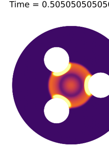
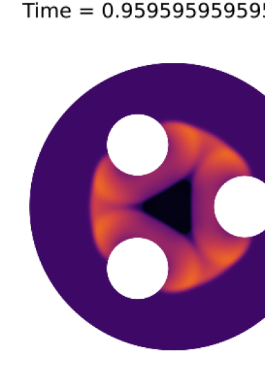
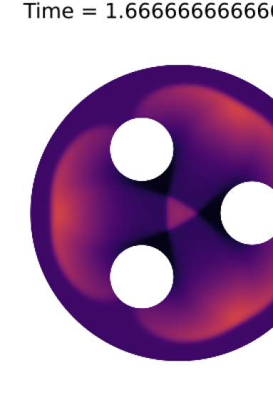
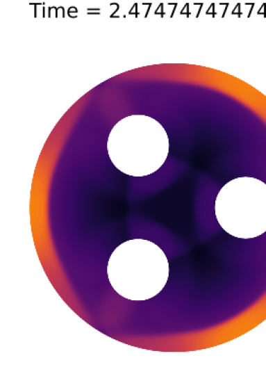
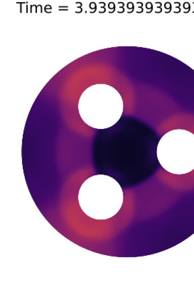
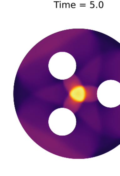
Figure 5. The computed pressure using the HLLC flux at various times. The color limits are taken from 0.008 to 0.25.

We additionally run the simulation until final time $t_{f}=7$ and compare the solutions computed using the local Lax-Friedrichs and HLLC flux Figure 6. We observe that the HLLC flux produces less dissipative solutions compared to the local Lax-Friedrichs flux.

(a) Lax-Friedrichs, $t=0.583$

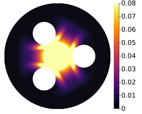
(b) HLLC, $t=0.583$

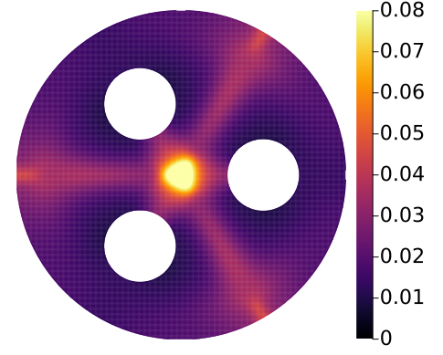
(c) Lax-Friedrichs, $t=4.67$

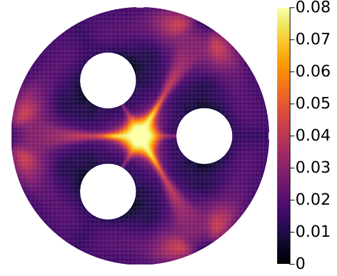
(d) HLLC, $t=4.67$

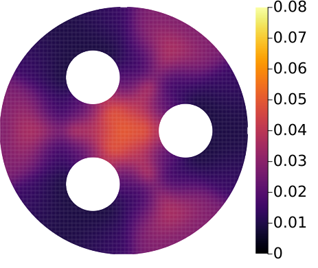
(e) Lax-Friedrichs, $t=5.54167$

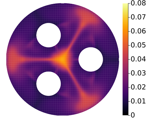
(f) HLLC, $t=5.54167$

Figure 6. Comparison of the density $\rho$ at different times using Lax-Friedrichs and HLLC fluxes.

7   Conclusion

By using the concept of summation by parts, we were able to create first differentiations that did not require a mesh but only a notion of adjacency. Upon picking a suitable notion of adjacency, namely the Euclidean Radius, we were able to efficiently create such operators. Using these SBP operators, we create a mesh-free numerical method using a flux-based formulation to numerically approximate non-linear conservation laws. The method performs reasonably well and is often first order given sufficient smoothness.

For reproducibility purposes, please refer to the GitHub repository in [15] for the codebase used to generate the SBP operators and the numerical results.

8   Acknowledgments

The authors gratefully acknowledge support by the National Science Foundation under award NSF DMS-2231482. Chan was also supported by DMS-1943186.

References

- [1] Ivo Babuška and A Kadir Aziz. On the angle condition in the finite element method. SIAM Journal on Numerical Analysis, 13(2):214–226, 1976.
- [2] Paul Batten, Nicholas Clarke, Claire Lambert, and Derek M Causon. On the choice of wavespeeds for the hllc riemann solver. SIAM Journal on Scientific Computing, 18(6):1553–1570, 1997.
- [3] Jeff Bezanson, Alan Edelman, Stefan Karpinski, and Viral B Shah. Julia: A fresh approach to numerical computing. SIAM review, 59(1):65–98, 2017.
- [4] Paul T Boggs, Alan Althsuler, Alex R Larzelere, Edward J Walsh, Ruuobert L Clay, and Michael F Hardwick. DART system analysis. Technical report, Sandia National Laboratories (SNL), Albuquerque, NM, and Livermore, CA …, 2005.
- [5] Kwan-Yu Edmond Chiu, Qiqi Wang, Rui Hu, and Antony Jameson. A Conservative Mesh-Free Scheme and Generalized Framework for Conservation Laws. SIAM Journal on Scientific Computing, 34(6):A2896–A2916, 2012.
- [6] Sidafa Conde, Imre Fekete, and John N Shadid. Embedded error estimation and adaptive step-size control for optimal explicit strong stability preserving Runge–Kutta methods. arXiv preprint arXiv:1806.08693, 2018.
- [7] Colin J Cotter. Compatible finite element methods for geophysical fluid dynamics. Acta Numerica, 32:291–393, 2023.
- [8] Stephen F Davis. Simplified second-order Godunov-type methods. SIAM Journal on Scientific and Statistical Computing, 9(3):445–473, 1988.
- [9] Ulrik S Fjordholm, Siddhartha Mishra, and Eitan Tadmor. Arbitrarily high-order accurate entropy stable essentially nonoscillatory schemes for systems of conservation laws. SIAM Journal on Numerical Analysis, 50(2):544–573, 2012.
- [10] Bengt Fornberg and Natasha Flyer. Solving PDEs with radial basis functions. Acta Numerica, 24:215–258, 2015.
- [11] Jan Glaubitz and Jonah A Reeger. Towards stability results for global radial basis function based quadrature formulas. BIT Numerical Mathematics, 63(1):6, 2023.
- [12] Jean-Luc Guermond, Bojan Popov, and Ignacio Tomas. Invariant domain preserving discretization-independent schemes and convex limiting for hyperbolic systems. Computer Methods in Applied Mechanics and Engineering, 347:143–175, 2019.
- [13] Jason E. Hicken, David C. Del Rey Fernández, and David W. Zingg. Multidimensional Summation-by-Parts Operators: General Theory and Application to Simplex Elements. SIAM Journal on Scientific Computing, 38(4):A1935–A1958, 2016.
- [14] The MathWorks Inc. Kdtreesearcher, 2010a.
- [15] Samuel Kwan Jesse Chan. Reproducibility Repository for “A robust first order meshfree method for time-dependent nonlinear conservation laws”. https://github.com/jlchan/paper-meshless-idp-2024, Oct 2024.
- [16] Aaron Katz and Venkateswaran Sankaran. Mesh quality effects on the accuracy of CFD solutions on unstructured meshes. Journal of Computational Physics, 230(20):7670–7686, 2011.
- [17] Johannes Franciscus Bernardus Maria Kraaijevanger. Contractivity of Runge-Kutta methods. BIT Numerical Mathematics, 31(3):482–528, 1991.
- [18] Randall J LeVeque. Finite volume methods for hyperbolic problems, volume 31. Cambridge university press, 2002.
- [19] Randall J LeVeque and Randall J Leveque. Numerical methods for conservation laws, volume 214. Springer, 1992.
- [20] Yimin Lin, Jesse Chan, and Ignacio Tomas. A positivity preserving strategy for entropy stable discontinuous Galerkin discretizations of the compressible Euler and Navier-Stokes equations. Journal of Computational Physics, 475:111850, 2023.
- [21] Konstantin Lipnikov, Gianmarco Manzini, and Mikhail Shashkov. Mimetic finite difference method. Journal of Computational Physics, 257:1163–1227, 2014.
- [22] Brendan O’Donoghue, Eric Chu, Neal Parikh, and Stephen Boyd. SCS: Splitting conic solver, version 3.2.6. https://github.com/cvxgrp/scs, November 2023.
- [23] Christopher Rackauckas and Qing Nie. Differentialequations. jl–a performant and feature-rich ecosystem for solving differential equations in julia. Journal of open research software, 5(1):15–15, 2017.
- [24] Hendrik Ranocha, Lisandro Dalcin, Matteo Parsani, and David I Ketcheson. Optimized Runge-Kutta methods with automatic step size control for compressible computational fluid dynamics. Communications on Applied Mathematics and Computation, 4(4):1191–1228, 2022.
- [25] Hendrik Ranocha, Michael Schlottke-Lakemper, Andrew Ross Winters, Erik Faulhaber, Jesse Chan, and Gregor Gassner. Adaptive numerical simulations with Trixi.jl: A case study of Julia for scientific computing. Proceedings of the JuliaCon Conferences, 1(1):77, 2022.
- [26] Michael Schlottke-Lakemper, Andrew R Winters, Hendrik Ranocha, and Gregor J Gassner. A purely hyperbolic discontinuous Galerkin approach for self-gravitating gas dynamics. Journal of Computational Physics, 442:110467, 06 2021.
- [27] Jonathan Shewchuk. What is a good linear finite element? Interpolation, conditioning, anisotropy, and quality measures (preprint). University of California at Berkeley, 2002, 2002.
- [28] Igor Tominec, Elisabeth Larsson, and Alfa Heryudono. A least squares radial basis function finite difference method with improved stability properties. SIAM Journal on Scientific Computing, 43(2):A1441–A1471, 2021.
- [29] Igor Tominec and Murtazo Nazarov. Residual viscosity stabilized RBF-FD methods for solving nonlinear conservation laws. Journal of Scientific Computing, 94(1):14, 2023.
- [30] Eleuterio F Toro. The hllc riemann solver. Shock waves, 29(8):1065–1082, 2019.
- [31] Eleuterio F. Toro, M. Spruce, and William Speares. Restoration of the contact surface in the HLL-Riemann solver. Shock Waves, 4:25–34, 1994.
- [32] Nathaniel Trask, Pavel Bochev, and Mauro Perego. A conservative, consistent, and scalable meshfree mimetic method. Journal of Computational Physics, 409:109187, 2020.
- [33] Nathaniel Trask, Pavel Bochev, and Mauro Perego. A conservative, consistent, and scalable meshfree mimetic method. Journal of Computational Physics, 409:109187, 2020.
- [34] Lloyd N Trefethen and JAC Weideman. The exponentially convergent trapezoidal rule. SIAM review, 56(3):385–458, 2014.
- [35] Jacobus J.W. van der Vegt and H. van der Ven. Slip flow boundary conditions in discontinuous Galerkin discretizations of the Euler equations of gas dynamics. In H.A. Mang and F.G. Rammenstorfer, editors, Proceedings of the 5th World Congress on Computational Mechanics (WCCM V), number NLR-TP in Technical Publications, pages 1–16. National Aerospace Laboratory, NLR, July 2002.
- [36] Xinhui Wu, Nathaniel Trask, and Jesse Chan. Entropy stable discontinuous Galerkin methods for the shallow water equations with subcell positivity preservation. Numerical Methods for Partial Differential Equations, page e23129, 2024.
- [37] Miloš Zlámal. Curved Elements in the Finite Element Method. I. SIAM Journal on Numerical Analysis, 10(1):229–240, 1973.