Classifying Order-Two Spatial Symmetries in Non-Hermitian Hamiltonians: Point-gapped AZ and AZ† Classes
Abstract
Crystalline topological insulators and superconductors have been a prominent topic in the field of condensed matter physics. These systems obey certain crystalline (spatial) symmetries that depend on the geometry of the lattice. The presence of spatial symmetries can lead to shift in the classification of ten-fold Altland–Zirnbauer class, given rise to new symmetry-protected topological phases. If the constraint of Hermiticity is broken, the classification expand into 38-fold. In this paper, following procedures in Hermitian systems, we classify all possible types of order-two spatial symmetries for point-gapped non-Hermitian systems within out of non-Hermitian topological classes. These classes are denoted by AZ and AZ† classes. We show that, similar to the Hermitian case, spatial symmetries will also lead to a shift in the classification of AZ and AZ† classes. There also exist novel symmetry-protected topological phases exclusive to point-gapped non-Hermitian Hamiltonians. Toy models are also given based on our classifications.
I Introduction
Topological insulators (TI) and superconductors (TSC) are some of the most intriguing discovery in condensed matter physics [1, 2, 3, 4]. Ref. [5] proposed a systematic way of classifying TI and TSC based on three internal symmetries: time-reversal symmetry (TRS), particle-hole symmetry (PHS), and chiral symmetry (CS). Together, they composed 10 different classes which are called periodic table of TI and TSC or Altland–Zirnbauer (AZ) symmetry class [6]. AZ classes give a complete classification of gapped phases of non-interacting fermionic systems with respect to internal symmetries. Different AZ classes are distinct from each other by some topological invariants that could exist in the presence or absence of certain internal symmetries. A phase transition between systems that have different topological invariants is achieved through the gap-closing of energy bands. For example, Chern insulator, which breaks TRS, can exist in 2D of class A [5, 7]. It has a invariant called the Chern number. When a system with a non-trivial Chern number is in contact with the vacuum (which has Chern number ), a gap closing of energy bands at the interface (or boundary) must happen. The states that localized at the boundary that closed the energy gap are the chiral edge states of Chern insulators. Similarly, quantum spin hall effect, which requires the existence of spinful TRS, can exist in class AII. It has a invariant called Kane-Mele invariant [8, 9]. When a non-trivial quantum spin hall system is in contact with the vacuum, helical edge states appear at the interface. These edge modes show that topological numbers can predict the phenomena of quantum systems.
The boundary of a system can be more generally understand in the context of topological defects [10, 11, 12]. Topological defects are defined to be lattice dislocation and disinclination that cannot be gapped out by continuous deformation. Under the protection of symmetries, defects may also host gapless topological modes. Therefore, under this view, boundary of a system is just another form of defects.
Meanwhile, Ref. [13, 14] discovered TIs that are based on inversion and crystalline symmetries, which are non-local spatial symmetries that depends on the geometry of the lattice. And, as shown in Ref. [13, 14], non-trivial TIs exist under the protection of spatial symmetries which are outside the classification of AZ symmetry classes. Therefore, a complete classification that includes spatial symmetries is called for. Works that classifies AZ symmetry class in addition to spatial symmetries are Ref. [15, 12, 16, 17, 18, 19, 20].
Another intriguing topics discovered in recent years is non-Hermitian (NH) TIs and TSCs. These systems break the conventional condition that the Hamiltonian describing the system must be Hermitian. A Hermitian Hamiltonian means the energy of the system is conserved. NH Hamiltonians counts in the exchange of energy between the original system and the environment, resulting in an exotic phenomenon called non-Hermitian skin effect (NHSE) [21, 22, 23, 24]. NHSE is protected by a invariant called winding number. When a system with non-trivial winding number is in contact with the vacuum, all states will localize at the boundary. This phenomenon is unique to NH systems which received vast attention in the recent years [25, 26, 27, 28, 29, 30, 31, 32, 33, 34, 35, 36]. Another interesting aspect of non-Hermiticity is that every internal symmetries would split into two (See Sec. III): TRS splits into TRS and TRS†; PHS splits into PHS and PHS†; CS splits into CS and sub-lattice symmetry (SLS). A complete classification of NH Hamiltonian is made in Ref. [24, 37] shortly after the topological invariant of NHSE is discovered. The bifurcation of internal symmetries results in 38 different classes, which greatly enriched the phenomenon of TIs and TSCs. Although much attention has been put into NH systems, little progress has been made to include spatial symmetries in the 38-fold classification. In this paper, following Ref.[12] which classify all order-two spatial symmetries for Hermitian Hamiltonians, we aim to incorporate order-two spatial symmetries into the classification of out of classes of NH Hamiltonians.
This paper is organized as the following: in Sec, II, we review the topological classification of Hermitian Hamiltonian without and with order-two spatial symmetries. In Sec. III, we review the classification of point-gapped NH Hamiltonians without order-two spatial symmetries. In Sec. IV, we introduce the classification scheme for point-gapped Hamiltonians of out of classes with spatial symmetries. Periodic tables for spatial symmetries are introduced in Sec. V. Finally, in Sec. VI, we introduce several examples to illustrate our classification. We conclude the paper with several remarks in Sec. VII. Mathematical details are provided in Appendix.
II Classification of order-two spatial symmetry for Hermitian Hamiltonians
To understand the process of classification of spatial symmetries in NH systems, we first review the classification of stable equivalent Hermitian Hamiltonian and spatial symmetries of Hermitian systems.
II.1 Review of topological defects and group classification of stable equivalent Hermitian Hamiltonians
First, we briefly review the process of including topological defects into the classification. In the absence of defects, we consider Hamiltonians that are defined on -dimensional Brillouin zone (BZ) which is a -Torus . In general, we may consider BZ as a simpler space which is a -sphere. This substitution will not affect the strong topological invariants [12].
Topological defects are defined to be discontinuity or distortion in lattices that cannot be removed. This discontinuity may be a point, a line, or a surface. In real space, we let a -dimensional sphere surrounds the defects. Combining with the -dimensional BZ, the total space of classification is given by . group classification is a common method for classifying topological invariants for topological insulators and superconductors in different dimensions [10, 12, 15, 7]. The classification of stable equivalent Hamiltonian is then equivalent to the classification of maps from base space of a dimensional sphere to the classifying space of Hamiltonian . This belongs to the problem of homotopy classification. As we will see, this classification can be simplified by considering the group , which is the zeroth homotopy group of classifying space. As we will see, the group in fact has an Abelian group structure, which allows us to classify Hamiltonians that are topologically distinct from each other.
We consider Hamiltonians that are gapped in the bulk i.e. far away from defects. This gap is often chosen to be the Fermi level. Two Hamiltonians are considered topologically equivalent if they can be continuously deformed into each other without closing the band gap. This means the two Hamiltonians have the same topological invariants. This allows us to deform a given Hamiltonian into two flat bands without closing the band gap: all the () bands below (above) the Fermi level are deformed into the same energy (). Then, according to the symmetries that the Hamiltonian has, we can find the classifying space of this Hamiltonian. Then by computing of the classifying space, we can derive the topological invariant of the corresponding Hamiltonian in dimension. Topological invariants in higher dimension can be found by using the dimensional hierarchy, which we will introduce later in Eqs. (2) and (3).
Throughout the paper, we consider Hamiltonians that are stable equivalent: Hamiltonian and are stable equivalent if they can be continuously deformed into each other by adding trivial bands. This ensures that the dimension of the Hamiltonian will not affect the classification. In other words, the addition of trivial bands will not affect the topology of the Hamiltonian (Hamiltonians that violate this condition are called Fragile insulators or Hopf insulators which we will not discuss in this paper [38, 39, 40, 41, 42, 43]). This allows us to identify a set of Hamiltonian that includes all Hamiltonians that are stable equivalent to . We define the addition of two sets to be , where is the direct sum. Then the inverse of is given by , where is the set of trivial Hamiltonians. Since we are discussing stable equivalent Hamilonians, the addition of to any Hamiltonians will not change the set it belongs to i.e. . We see that acts as the identity in this operation. The direct sum is associative and commutative. Therefore, different classes of Hamiltonians form an Abelian group, which is called group.
Now we consider symmetries that separate these classes. The internal symmetries that govern Hermitian Hamiltonians are
| (1) |
which are called Time-Reversal Symmetry (TRS), Particle-hole symmetry (PHS), and Chiral Symmetry (CS), respectively. Specifically, and are antiunitary operators, meaning they can be written in the form of a unitary matrix times complex conjugate operator . And is a unitary operator. The combination of these symmetries will result in classes. If no antiunitary symmetries (TRS and PHS) are present, the symmetry classes are called the complex AZ class. Since in the absence of complex conjugate operator , the Clifford generators that generate the classifying space of each class is defined up to a phase. So these generators are in general complex. Hence the name complex AZ class is given to classes without antiunitary symmetries. If one or both antiunitary symmetries are present, the symmetry classes are called real AZ class. In this case, generators of each class can only be real or imaginary. Hence the name real AZ class.
Having discussed group and symmetries that govern each class, we now show the group relationship of each class. The AZ symmetry classes may summarized as [10]
| (2) |
for complex AZ classes (A and AIII), and
| (3) |
for real AZ classes (the rest of the eight classes). The and are classifying space of the Hamiltonians. Their exact expressions can be found in Ref. [5]. The number labels the symmetry classes. Notice that complex AZ class has periodicity i.e. the classifying space obeys . Hence is defined mod 2 in Eq. (2). This periodicity is the origin of two complex AZ classes. Similarly, for real AZ class, the classifying space obeys . Hence is defined mod 8 in Eq. (3). This periodicity gives eight real AZ classes. Periodicity of Eqs. (2) and (3) are called Bott periodicity, which is an essential mathematical property of group in the classification of TIs and TSCs. The resulting table from Eqs. (2) and (3) is the AZ symmetry class, which we do not repeat it here.
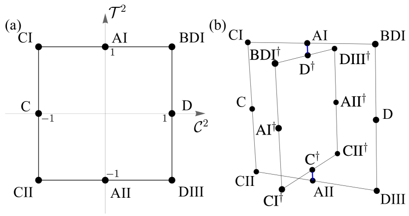
Finally, we remark that Eqs. (2) and (3) are referred to as dimensional hierarchy of AZ symmetry class, which is first proved in Ref. [10]. A neat way to visualize Eq. (3) is by putting real AZ classes on a coordinate where () axis indicates the value of (). We plot this visualization in Fig. 1 (a). In this way, eight real AZ classes would form a ”clock”. In Sec. III, we also provide a similar relation and visualization for point-gapped Hamilonians.
II.2 Classification under order-two spatial symmetry
The spatial symmetries (or crystalline symmetries) are symmetries that are dependent on the geometry of the lattice [15, 12, 17, 18]. In the paper, we consider spatial symmetries that are of order two, meaning apply them twice on the Hamiltonian will keep the Hamiltonian unchanged. These spatial symmetries can be unitary () or antiunitary (). Furthermore, they can commute or anti-commute with the Hamiltonians. For the later, a bar is placed on top of the spatial operator. To sum up, possible order-two spatial symmetries for Hermitian systems are
| (4) |
where () denotes k that are flipped (unchanged) under unitary symmetries. Similar notation also applies to r. Pioneer works that classify order-two spatial symmetries as an addition to internal symmetries are Ref. [12, 15]. These additional spatial symmetries will add a finer structure to the dimensional hierarchy Eqs. (2), (3) that may add or remove certain topological invariants.
In the following sections, we will repeat this process for point-gapped NH Hamiltonians. Before that, we first introduce the 38-fold classification of NH Hamiltonians in the next sections.
| Symmetry class | C.L. | |||||||||||||||
| Complex AZ | A | 1 | ||||||||||||||
| AIII | 0 | |||||||||||||||
| Real AZ | AI | 1 | ||||||||||||||
| BDI | 2 | |||||||||||||||
| D | 3 | |||||||||||||||
| DIII | 4 | |||||||||||||||
| AII | 5 | |||||||||||||||
| CII | 6 | |||||||||||||||
| C | 7 | |||||||||||||||
| CI | 0 | |||||||||||||||
| Real | 7 | |||||||||||||||
| 0 | ||||||||||||||||
| 1 | ||||||||||||||||
| 2 | ||||||||||||||||
| 3 | ||||||||||||||||
| 4 | ||||||||||||||||
| 5 | ||||||||||||||||
| 6 | ||||||||||||||||
III Structure of -fold classification of NH Hamiltonian
We consider internal symmetries of NH Hamiltonians. Due to non-Hermiticity, will bifurcate into and . Following notations in Ref. [24], internal symmetries for NH Hamiltonians bifurcate into
| (5) |
where SLS denotes sub-lattice symmetry. The combination of these symmetries will result in independent classes. In this paper, we consider classes without SLS. As we will see, combinations of other symmetries will results in two sets of classes that are similar to Hermitian AZ symmetry classes.
We now comment on the structure of classes without SLS. The combination of TRS, PHS, and CS will result in symmetry classes that are similar to AZ symmetry class for Hermitian Hamiltonians (See Table 1). These classes are called as AZ class for NH Hamiltonians. From now on, by AZ class, we mean AZ class for NH Hamiltonians from Table 1. Next, consider the combination of TRS† and PHS†. Symmetry classes formed by these symmetries are called AZ† classes. They constitute classes in total. Furthermore, if only PHS† is present (class D† and C† in Table 1), PHS† can be transformed into to TRS (class AI and AII) and vice versa [44]. To see this, consider a Hamiltonian that obeys PHS† (). Then obeys TRS with operator :
| (6) |
The mapping can be understood as a 90 degree rotation of energy spectrum on the complex plane. This operation does not change the topology of Hamiltonian . Therefore, we see that class D† (C†) is unified with AI (AII). As we will see in Appendix. A, this unification will have some consequences on the dimensional hierarchy of AZ and AZ† classes. Therefore, there are independent symmetry classes in AZ†. Similar to Hermitian classification, class A and AIII are complex classes, meaning they can be represented by complex Clifford algebra, while the rest of the classes are real (due to the existence of complex conjugate operator in and ), meaning they can be represented by real Clifford algebra. In Table 1, we label AZ (AZ†) class by ().
The addition of SLS to AZ classes will result in additional symmetry classes. So there are symmetry classes in total. The -fold SLS classes can be further divided into five sub-classes (See Ref. [24] for details). However, since the SLS classes are rarely explored in current literature, we do not consider them in this paper.
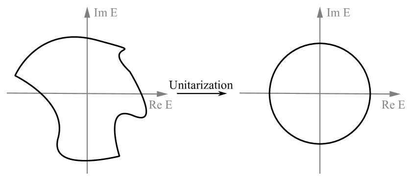
As we are interested in point gap in this paper, we also briefly review the classification schemes for point gapped Hamiltonians. For a given point-gapped Hamiltonian , we can continuously deform it into a unitary matrix without closing the point gap. This process is called unitary flattening [24, 45], which we show in Fig. 2. We may then consider the extended Hermitian Hamiltonian
| (7) |
If original Hamiltonian obeys symmetries in Eq. (5), the extended Hamiltonian then obeys
| (8) |
Furthermore, Eq. (7) also obeys an additional CS
| (9) |
For clearance, Eq. (9) will be called symmetry in the rest of the paper. Notably, symmetry arise since we are using extended Hamiltonian for the classification. In fact, the existence of is the biggest difference between classifying a Hermitian Hamiltonian and a point-gapped NH Hamiltonian. Now, the classification of point-gapped Hamiltonian is mapped to the classification of extended Hermitian Hamiltonian (7) with symmetries (8) and (9). This allows us to use the classification process on for Hermitian Hamiltonians discussed in Sec. II. The group relationships are given by
| (10) |
for complex AZ classes and
| (11) |
for real AZ classes and finally
| (12) |
for AZ† classes; The superscript is put to distinguish group of AZ† class from that of AZ class. The unification of AI and D†, AII and C† also gives
| (13) |
We proof these relationships rigorously in Appendix A.
The dimensional hierarchy of AZ and AZ† class for point-gapped Hamiltonian can be understood as two ”clocks”: one for AZ and the other for AZ†. Two clocks are connected by the mapping Eq. (6). We draw these two clocks in Fig. 1.
In order to include spatial symmetries in the classification, we also need to consider the extension of spatial symmetries. In the following, we focus on order-two spatial symmetries as an additional symmetry to -fold AZ and AZ† classes in Table 1.
IV Order-two spatial symmetries in AZ and AZ†
Similar to the bifurcation of internal symmetries, each type of spatial symmetry Eqs. (4) will also bifurcate into two. We label them according to
| (14) |
where and refer to conventional and generalized spatial symmetries, respectively; () denotes k that are flipped (unchanged) under unitary symmetries. Similar notation also applies to r. Similar to the extension of internal symmetries for point-gapped Hamiltonians in Eq. (8), to include spatial symmetries in the classification, we also consider the extension of Eq. (14). For the conventional spatial symmetries (those with at the front), their extensions are given by
| (15) |
where , or . For generalized spatial symmetries (those with at the front), their extensions are given by
| (16) |
where , or . These extended spatial symmetries would have the same effect on in Eq. (7) as original spatial symmetries on original . Therefore, we again mapped the classification problem of point gapped Hamiltonian to that of extended Hamiltonian (7).
Before continuing, we would like to comment on an important effect of the symmetry [Eq. (9)] that would ”unify” certain spatial symmetries. As an example, consider spatial symmetry and its extension , which operate on extended Hermitian Hamiltonian
| (17) |
Combining with symmetry, which is always present for point gap Hamiltonians, will result in the following symmetry:
| (18) |
Therefore, we see that has the exact same expression as on Hamiltonian. Hence symmetry would map a spatial symmetry that commutes with extended Hamiltonian to its anti-commuting counterpart and vice versa. In this sense, symmetry ”unifies” commuting and anti-commuting symmetries. However, this unification is not physical. We can understand this fact in two ways: First, symmetry is only present for extended Hamiltonians instead of the original Hamiltonians. Therefore, this unification is only a by-product of adopting extended Hamiltonian formalism. Second, if we write explicitly, we would find
| (19) |
which does not follow the form of Eq. (15). Hence, even if commuting symmetries will always have the same classification as anti-commuting symmetries, we should bear in mind that such unification is only a mathematical coincidence, which does not implies that both symmetries exist in the original system. However, since the classification problem is mapped to , symmetry will cause the same classification for and , as they have the same effect on up to a multiplication of . In the following sections, we will discuss the effects of symmetry in more detail.
In the present of internal symmetries Eqs. 5, not all these spatial symmetries are independent. Following the process of Ref. [12], we first find equivalent spatial symmetries under the presenting internal symmetries for a certain symmetry class, then we give a finer classification of the corresponding symmetry classes due to spatial symmetries.
IV.1 Complex classes A and AIII with order-two unitary symmetry
We first consider classes A and AIII in the present of order-two unitary symmetry ( and in Eqs. (14)). Due to the absent of antiunitary symmetries, symmetries and are defined up to a phase that does not affect the classification. Therefore, we may set .
For class A in which no internal symmetries are present, all and are independent of each other.
Now consider class AIII where only CS in Eq. (5) is present. The CS operator might commute or anti-commute with spatial symmetry operators. For example,
| (20) |
where . To indicate this commutation relation between operators, we put a subscript to spatial operator such that . Next, we investigate the combination of CS operator and spatial symmetry operators. Based on the effect of CS in Eq. (5), CS would flip spatial symmetries to and add another minus sign. Therefore, we see that and . We summarize all possible order-two unitary symmetries for A and AIII in Table 2.
Notice that all the conclusions up until now are applicable to all kinds of energy gaps. Following the discussion at the beginning of Sec. IV, by considering the effect of symmetry, we limit our scope to point gap. As an example, consider in class A. Then will have the same effect on extended Hamiltonian as . As another example, consider in class AIII. Notice that anti-commute with extended CS operator . Therefore, will have the same effect on the extended Hamiltonian as . By going over all possible order-two unitary symmetries for A and AIII in similar process, we can find all symmetries that are independent or related to each other through symmetry. We label those symmetries that are independent by and , where is defined mod. For simplicity, we abbreviate them into and in Table 2. We emphasize again that such connection is a purely mathematical coincidence which does not imply both symmetries exist in the system.
In Appendix B, we show the following dimensional hierarchy of complex AZ classes with unitary spatial symmetries
| (21) |
where the superscript indicates this relationship works for unitary spatial symmetries. Recall that is the dimension of the system and is the dimension of the sphere surrounds the defect. Here, () is the dimension of the system(sphere) that is being flipped under the spatial symmetry. Furthermore,
| (22) |
which we show in Appendix D using Clifford Algebra. We record some properties of Clifford Algebra in Appendix C. For both Eqs, and are defined mod. Eqs. 21 and 22 allow us to conclude periodic table for complex AZ class with unitary spatial symmetries, which we will introduce in Sec. V.
| Class | ||
|---|---|---|
| A | ||
| A | ||
| AIII | ||
| AIII |
IV.2 Complex classes A and AIII with order-two antiunitary symmetry
Now we consider the presence of antiunitary spatial symmetries [ and in Eqs. (14)].
For both and types of antiunitary symmetry, we use superscript to denote their squared value i.e. , ; The subscript (if present) denote their commutation relationship between CS operator i.e. . Furthermore, in the present of CS, CS would flip to and add another minus sign. Therefore, the following relationship hold .
Similar to the antiunitary spatial symmetry with Hermitian Hamiltonians (See Ref. [12]), the presence of antiunitary spatial symmetries will map complex classes A and AIII into one of real AZ and AZ† classes. To see this, one may consider antiunitary symmetries as effective TRS(†) or PHS(†) symmetries.
As an example, consider the addition of to class A (First row of Table 3), which add the symmetry
| (23) |
to class A. If we treat as ”momentum” and as ”positions”, we see that Eq. (23) has exactly the same form as TRS with . Now, the dimension of the BZ is given by the combined dimension of and , which is . The dimension of the sphere that surrounds the defect is given by the combined dimension of and , which is . Therefore, with the addition of , class A is mapped to class AI.
As another example, consider the addition of to class AIII (Second row of Table 3). By considering as ”momentum” , the antiunitary symmetry has the same form as PHS with . Next, consider . The CS symmetry takes Hermitian conjugate of the Hamiltonian again and give another minus sign i.e. . Finally, since and commute, we have . This suggest we can define which has the same form as TRS. We see that the addition of will map AIII to BDI.
Following similar process, we enumerate all possible types of order-two antiunitary symmetries in class A and AIII and their mapped classes in Table 3.
Finally, we comment on the effect of symmetry. As an example, we consider again in class AI. Due to the symmetry, the operator has the same effect on extended Hamiltonian as . According to Table 3, symmetry would unify class AI and D† i.e. these two classes would have the same topological invariants and classification. Indeed, in the 38-fold classification, AI and D† have the same classification under point gap. We mark symmetry classes that are equivalent under symmetry by identical symbols at the end of the symmetry operator in Table 3. Notice that our results are consistent with 38-fold classification in Ref. [24] i.e. the mapped classes marked with same symbol in Table 3 have the same topological classification under point gap.
The dimensional hierarchy of complex AZ class with antiunitary spatial symmetry is thus given by
| (24) |
where is given in Eq. (11).
| Class | Symmetry | Map to class |
|---|---|---|
| A | AI | |
| AIII | BDI | |
| A | D | |
| AIII | DIII | |
| A | AII | |
| AIII | CII | |
| A | C | |
| AIII | CI | |
| A | AI† | |
| AIII | BDI† | |
| A | D† | |
| AIII | DIII† | |
| A | AII† | |
| AIII | CII† | |
| A | C† | |
| AIII | CI† |
IV.3 Real AZ classes with order-two symmetry
| AZ class | |||||
|---|---|---|---|---|---|
| 1 | AI | (, ) | (, ) | (, ) | (, ) |
| (, ) | (, ) | (, ) | (, ) | ||
| (, ) | (, ) | (, ) | (, ) | ||
| (, ) | (, ) | (, ) | (, ) | ||
| 2 | BDI | (, , , ) | (, , , ) | (, , , ) | (, , , ) |
| (, , , ) | (, , , ) | (, , , ) | (, , , ) | ||
| (, , , ) | (, , , ) | (, , , ) | (, , , ) | ||
| (, , , ) | (, , , ) | (, , , ) | (, , , ) | ||
| 3 | D | (, ) | (, ) | (, ) | (, ) |
| (, ) | (, ) | (, ) | (, ) | ||
| (, ) | (, ) | (, ) | (, ) | ||
| (, ) | (, ) | (, ) | (, ) | ||
| 4 | DIII | (, , , ) | (, , , ) | (, , , ) | (, , , ) |
| (, , , ) | (, , , ) | (, , , ) | (, , , ) | ||
| (, , , ) | (, , , ) | (, , , ) | (, , , ) | ||
| (, , , ) | (, , , ) | (, , , ) | (, , , ) | ||
| 5 | AII | (, ) | (, ) | (, ) | (, ) |
| (, ) | (, ) | (, ) | (, ) | ||
| (, ) | (, ) | (, ) | (, ) | ||
| (, ) | (, ) | (, ) | (, ) | ||
| 6 | CII | (, , , ) | (, , , ) | (, , , ) | (, , , ) |
| (, , , ) | (, , , ) | (, , , ) | (, , , ) | ||
| (, , , ) | (, , , ) | (, , , ) | (, , , ) | ||
| (, , , ) | (, , , ) | (, , , ) | (, , , ) | ||
| 7 | C | (, ) | (, ) | (, ) | (, ) |
| (, ) | (, ) | (, ) | (, ) | ||
| (, ) | (, ) | (, ) | (, ) | ||
| (, ) | (, ) | (, ) | (, ) | ||
| 0 | CI | (, , , ) | (, , , ) | (, , , ) | (, , , ) |
| (, , , ) | (, , , ) | (, , , ) | (, , , ) | ||
| (, , , ) | (, , , ) | (, , , ) | (, , , ) | ||
| (, , , ) | (, , , ) | (, , , ) | (, , , ) |
In this section, we consider the classification of real AZ classes with order-two spatial symmetries. Throughout this section, all Eqs. are also valid upon exchange ; The superscripts denote the squared value of the spatial operators, and the subscripts denote the commutation relationship between spatial operators and and . Throughout this paper, we take the convention that .
For class A and AII, we have the following equivalence symmetries
AI and AII ():
| (25) |
where the subscript denotes the commutation relationship between the operator and .
For class D and C, we have the following equivalence symmetries
D and C ():
| (26) |
where the subscript denotes the commutation relationship between the operator and .
Finally, for class BDI, DIII, CII, and CI, we have
BDI, DIII, CII, and CI ( and ):
| (27) |
where the first (second) subscript () indicates the commutation relationship between the operator and ().
By going over all possible combinations of , we summarize possible order-two spatial symmetries for real AZ classes in Table 4.
Next, we discuss the effect of symmetry. Similar to the previous case for complex AZ classes, symmetry would ”unify” some spatial symmetries in Table 4. As an example, consider class AI with spatial symmetry . Recall that the operator in Eq. (9) anti-commutes with generalized spatial symmetries Eq. (16). Therefore, has the same classification as . We may repeat this process for all classes in Table 4. For each class, we label symmetries that are independent by , where is defined mod. We abbreviate these symbols into and label them at the end of the circular bracket in Table 4.
In Appendix B, we show that the group for real AZ classes with spatial symmetries obey the following relationship
| (28) |
where the superscript indicates this relationship works for both unitary and anti-unitary spatial symmetries. Furthermore,
| (29) |
which we show in Appendix D using Clifford Algebra. For both Eqs. is defined mod while is defined mod.
IV.4 Real AZ† classes with order-two symmetry
| AZ† class | |||||
|---|---|---|---|---|---|
| 7 | AI† | (, ) | (, ) | (, ) | (, ) |
| (, ) | (, ) | (, ) | (, ) | ||
| (, ) | (, ) | (, ) | (, ) | ||
| (, ) | (, ) | (, ) | (, ) | ||
| 0 | BDI† | (, , , ) | (, , , ) | (, , , ) | (, , , ) |
| (, , , ) | (, , , ) | (, , , ) | (, , , ) | ||
| (, , , ) | (, , , ) | (, , , ) | (, , , ) | ||
| (, , , ) | (, , , ) | (, , , ) | (, , , ) | ||
| 1 | D† | (, ) | (, ) | (, ) | (, ) |
| (, ) | (, ) | (, ) | (, ) | ||
| (, ) | (, ) | (, ) | (, ) | ||
| (, ) | (, ) | (, ) | (, ) | ||
| 2 | DIII† | (, , , ) | (, , , ) | (, , , ) | (, , , ) |
| (, , , ) | (, , , ) | (, , , ) | (, , , ) | ||
| (, , , ) | (, , , ) | (, , , ) | (, , , ) | ||
| (, , , ) | (, , , ) | (, , , ) | (, , , ) | ||
| 3 | AII† | (, ) | (, ) | (, ) | (, ) |
| (, ) | (, ) | (, ) | (, ) | ||
| (, ) | (, ) | (, ) | (, ) | ||
| (, ) | (, ) | (, ) | (, ) | ||
| 4 | CII† | (, , , ) | (, , , ) | (, , , ) | (, , , ) |
| (, , , ) | (, , , ) | (, , , ) | (, , , ) | ||
| (, , , ) | (, , , ) | (, , , ) | (, , , ) | ||
| (, , , ) | (, , , ) | (, , , ) | (, , , ) | ||
| 5 | C† | (, ) | (, ) | (, ) | (, ) |
| (, ) | (, ) | (, ) | (, ) | ||
| (, ) | (, ) | (, ) | (, ) | ||
| (, ) | (, ) | (, ) | (, ) | ||
| 6 | CI† | (, , , ) | (, , , ) | (, , , ) | (, , , ) |
| (, , , ) | (, , , ) | (, , , ) | (, , , ) | ||
| (, , , ) | (, , , ) | (, , , ) | (, , , ) | ||
| (, , , ) | (, , , ) | (, , , ) | (, , , ) |
Following similar steps as previous section, we derive equivalent symmetries for real AZ† classes in this section. All Eqs. in this section are also valid upon exchange . Throughout this paper, we take the convention that TRS† operator and PHS† operator commute: .
For class AI† and AII†, we have the following equivalent symmetries
AI† and AII† ():
| (30) |
where the subscript indicates the commutation relationship between spatial symmetries and TRS† operator .
For class D† and C†, we have
D† and C† ():
| (31) |
where the subscript indicates the commutation relationship of PHS† operator .
Finally, for class BDI†, DIII†, CII†, and CI†, we have
BDI†, DIII†, CII†, and CI†:
| (32) |
where the first (second) subscript indicates the commutation relationship between spatial symmetries and TRS† (PHS†).
By going over all possible combinations of , we summarize the equivalent symmetries in Table 5. Similar to real AZ classes, would unify certain spatial symmetries for AZ† class. The procedure to classify them is the same as AZ class. We label them by at the end of circular bracket in Table 5.
In Appendix B, we show the following group relationship for AZ† classes with spatial symmetries
| (33) |
where the superscript indicates this relationship works for both unitary and antiunitary spatial symmetries. Furthermore,
| (34) |
which we show in Appendix D using Clifford Algebra. For both Eqs, is defined mod while is defined mod
V Periodic table of spatial symmetries for point-gapped Hamiltonian
Having introduced the group of AZ and AZ† class in the presence of spatial symmetries, we are now ready to present their periodic table under spatial symmetries.
Each AZ (AZ†) class is labeled by (). The dimensional hierarchy for these parameters is controlled by the difference between spatial dimensions and the dimension of the -sphere that surrounds the defects: . The periodic table is given by ranging from to for each class (See Table 1). In the previous section, for each class, we give them a finer labeling in the presence of spatial symmetries, where is defined mod 2 for A and AIII or mod 4 for the rest of the classes. As we can see from group relationship we introduce at the end of each sub-section [Eqs. (21), (28), and (33)], the dimensional hierarchy for is controlled by , where () is the number of spatial dimension (dimension of -sphere that surrounds the defect) that is being flipped under spatial symmetry. In the following, we introduce periodic tables by ranging from to . This would give us four distinct tables. We summarize the result in table 6, 7, 8, and 9 for , respectively. In the following sections, we use specific examples to illustrate these topological invariants.
| Symmetry | Class | Classifying space | ||||||||
|---|---|---|---|---|---|---|---|---|---|---|
| A | ||||||||||
| AIII | ||||||||||
| A | ||||||||||
| AIII | ||||||||||
| AI,D† | ||||||||||
| BDI,DIII† | ||||||||||
| D,AII† | ||||||||||
| DIII,CII† | ||||||||||
| AII,C† | ||||||||||
| CII,CI† | ||||||||||
| C,AI† | ||||||||||
| CI,BDI† | ||||||||||
| AI,AI† | ||||||||||
| BDI,BDI† | ||||||||||
| D,D† | ||||||||||
| DIII,DIII† | ||||||||||
| AII,AII† | ||||||||||
| CII,CII† | ||||||||||
| C,C† | ||||||||||
| CI,CI† | ||||||||||
| AI,D,AII,C,AI†,D†,AII†,C† | ||||||||||
| BDI,DIII,CII,CI,BDI†,DIII†,CII†,CI† | ||||||||||
| AI,AII† | ||||||||||
| BDI,CII† | ||||||||||
| D,C† | ||||||||||
| DIII,CI† | ||||||||||
| AII,AI† | ||||||||||
| CII,BDI† | ||||||||||
| C,D† | ||||||||||
| CI,DIII† |
| Symmetry | Class | Classifying space | ||||||||
|---|---|---|---|---|---|---|---|---|---|---|
| A | ||||||||||
| AIII | ||||||||||
| A | ||||||||||
| AIII | ||||||||||
| AZ: AZ†: | AI,D† | |||||||||
| BDI,DIII† | ||||||||||
| D,AII† | ||||||||||
| DIII,CII† | ||||||||||
| AII,C† | ||||||||||
| CII,CI† | ||||||||||
| C,AI† | ||||||||||
| CI,BDI† | ||||||||||
| AZ: AZ†: | AI,D† | |||||||||
| BDI,DIII† | ||||||||||
| D,AII† | ||||||||||
| DIII,CII† | ||||||||||
| AII,C† | ||||||||||
| CII,CI† | ||||||||||
| C,AI† | ||||||||||
| CI,BDI† | ||||||||||
| AZ: AZ†: | AI,D† | |||||||||
| BDI,DIII† | ||||||||||
| D,AII† | ||||||||||
| DIII,CII† | ||||||||||
| AII,C† | ||||||||||
| CII,CI† | ||||||||||
| C,AI† | ||||||||||
| CI,BDI† | ||||||||||
| AZ: AZ†: | AI,D,AII,C,AI†,D†,AII†,C† | |||||||||
| BDI,DIII,CII,CI,BDI†,DIII†,CII†,CI† |
| Symmetry | Class | Classifying space | ||||||||
|---|---|---|---|---|---|---|---|---|---|---|
| AZ: AZ†: | AI,D,AII,C,AI†,D†,AII†,C† | |||||||||
| BDI,DIII,CII,CI,BDI†,DIII†,CII†,CI† | ||||||||||
| AZ: AZ†: | AI,D† | |||||||||
| BDI,DIII† | ||||||||||
| D,AII† | ||||||||||
| DIII,CII† | ||||||||||
| AII,C† | ||||||||||
| CII,CI† | ||||||||||
| C,AI† | ||||||||||
| CI,BDI† | ||||||||||
| AZ: AZ†: | AI,D† | |||||||||
| BDI,DIII† | ||||||||||
| D,AII† | ||||||||||
| DIII,CII† | ||||||||||
| AII,C† | ||||||||||
| CII,CI† | ||||||||||
| C,AI† | ||||||||||
| CI,BDI† | ||||||||||
| AZ: AZ†: | AI,D† | |||||||||
| BDI,DIII† | ||||||||||
| D,AII† | ||||||||||
| DIII,CII† | ||||||||||
| AII,C† | ||||||||||
| CII,CI† | ||||||||||
| C,AI† | ||||||||||
| CI,BDI† |
| Symmetry | Class | Classifying space | ||||||||
|---|---|---|---|---|---|---|---|---|---|---|
| AZ: AZ†: | AI,D† | |||||||||
| BDI,DIII† | ||||||||||
| D,AII† | ||||||||||
| DIII,CII† | ||||||||||
| AII,C† | ||||||||||
| CII,CI† | ||||||||||
| C,AI† | ||||||||||
| CI,BDI† | ||||||||||
| AZ: AZ†: | AI,D,AII,C,AI†,D†,AII†,C† | |||||||||
| BDI,DIII,CII,CI,BDI†,DIII†,CII†,CI† | ||||||||||
| AZ: AZ†: | AI,D† | |||||||||
| BDI,DIII† | ||||||||||
| D,AII† | ||||||||||
| DIII,CII† | ||||||||||
| AII,C† | ||||||||||
| CII,CI† | ||||||||||
| C,AI† | ||||||||||
| CI,BDI† | ||||||||||
| AZ: AZ†: | AI,D† | |||||||||
| BDI,DIII† | ||||||||||
| D,AII† | ||||||||||
| DIII,CII† | ||||||||||
| AII,C† | ||||||||||
| CII,CI† | ||||||||||
| C,AI† | ||||||||||
| CI,BDI† |
VI Examples
In this section, we give several concrete examples of toy models that demonstrate how to use our periodic table introduced in the previous section. Before introducing concrete models, we first discuss several preliminary considerations.
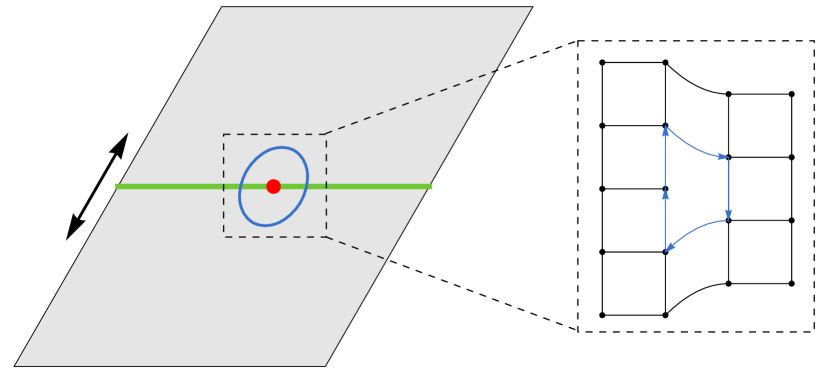
To simplify our discussion and also to be aligned with current interest within the field of non-Hermitian defects, we focus on the case of point defect in 2D [Fig. 3 (a)] protected by reflection symmetry. In this case, and the periodic table is table 6. Without loss of generality, we assume the model obeys reflection symmetry in direction. For a complete enumeration of defects for different , see Ref. [12].
Physically, a point defect on lattice is obtained by removing a site and reintroducing hopping for sites after the defect (Fig. 3 (b)). For a point-gapped non-Hermitian system in 2D, point defect is known to generate skin effects, which is referred to as dislocation non-Hermitian skin effect in previous works [33, 34, 35]. We see that, by this construction of point defects, the circle surrounds the point would give us a Burgers vector . In order to preserve periodic boundary condition (PBC), another defect with burgers vector pointing in the opposite direction must be introduced at the other end hoppings chains that are reintroduced. Since the defect is probing the topological property of sub-manifold , we see that for , the topological property of the defect is given by the sub-manifold .
Finally, to give a sharp contrast between models with and without reflection symmetries, we are investigating the reflection-symmetry-protected phases. By comparing table 6 and 1, we see that class AI† with class symmetry and class C with class symmetry are protected by the extra spatial symmetry with invariant ; Class DIII with class symmetry is also protected by the extra spatial symmetry with a invariant. If we break the relevant spatial symmetry (reflection in this case), the topological invariant will vanish since their original classification in Table 1 is trivial. By doing so, there are two possible ways the system will change: (i) the modes that are originally localized around the defect will be delocalized, or (ii) a line gap will open, in which case the topological property is governed by line gap instead of point gap. In this sense, the defects mode for point-gapped spectrum is protected by the reflection symmetry. On the other hand, for class D† with class symmetry, if the spatial symmetry is broken, we expect the defect mode and point gap remain the same since D† has a invariant for without spatial symmetry. In this case, the reflection symmetry does not protect the point gap or the defect modes.
In the following, we introduce four models in (Table 6) that would realize scenarios that we described above. They belong to class AI†, C, and D† with class reflection symmetry, and class DIII with class symmetry.
VI.1 Point defect in AI† protected by reflection symmetry
We build a two-dimensional AI† model that obeys reflection symmetry of the type . Following the construction of NHSE model [23], we stack an HN model with its AI† pair in direction with symmetry-preserving coupling in direction. The resulting model is
| (35) |
where is the two-band HN model
| (36) |
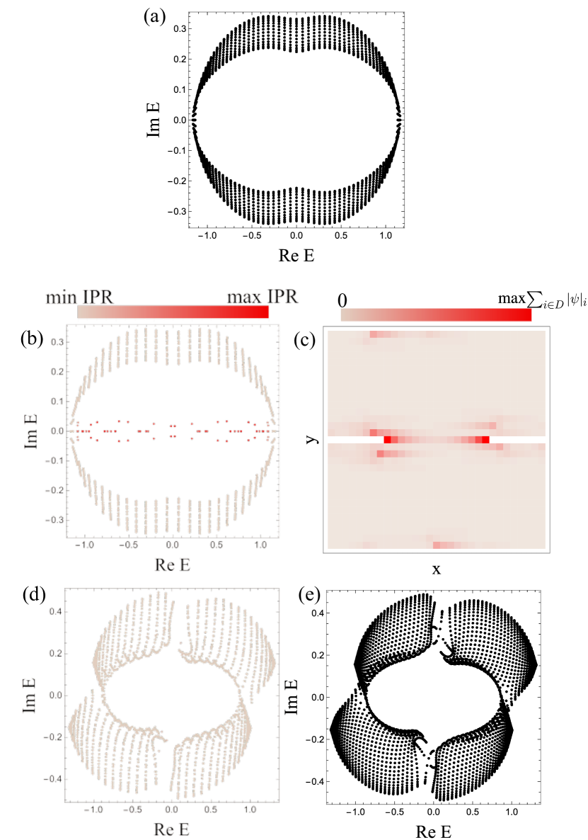
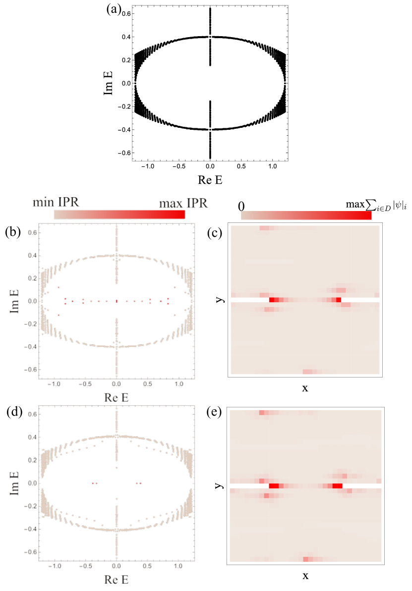
is the symmetry-preserving coupling in direction. are all real parameters. Model (35) obeys TRS† with . It also obeys the reflection such that . According to the classification table 5 and 6, this model belongs to the subclass of AI†. In the case of 2D with a point defect such that , this topological phases has a invariant which we will later show is given by the mirror winding number.
We plot the spectrum of model (35) in Fig. 4 (a) under full PBC. After introducing two defects for a HN chain in direction, in-gap states that are localized at the defect appear [Fig. 4 (b) and (c)]. As mentioned at the beginning of the section, in this construction, the Burgers vector is given by , which is probing the topological property of the sub-manifold . At , , Eq. (35) decoupled into two independent HN models with opposite winding numbers. We can diagonalize the resulting Hamiltonian into sectors that correspond to the eigenvalues of . This was automatically done for model (35). We are now left with
| (37) |
For each sectors of the above Hamiltonian, we can define a winding number
| (38) |
The invariant is given by the mirror winding number [46]
| (39) |
For model (35), we have since . In turn, this nontrivial mirror winding number gives rise to the localization of in-gap state around the defect. Notice that now the total winding number vanishes. Since is only well-defined under reflection symmetry while is always well-defined, we see that the topological phase of model (35) is protected by reflection symmetry. Mirror winding number is first proposed in Ref. [46] for NHSE protected by mirror symmetry (which is a different name of reflection symmetry). The mirror winding number is defined in a similar way as mirror Chern number [12].
The protection of reflection symmetry can also be seen by noticing that in the classification without reflection symmetry (Table 1), class AI† is trivial in the case . Therefore, by breaking reflection symmetry, we expect either the in-gap state to loss localization and become trivial or the system opens a line gap such that the classification changes. To show this explicitly, we introduce a reflection-symmetry-breaking term . As shown in Fig. 4 (d) and (e), the in-gap states vanish after the addition of a symmetry-breaking term for . Notice that for smaller , the in-gap states still exist. However, by increasing the value of the in-gap states would vanish without going through a phase transition. Thus, in-gap states after the addition of reflection-symmetry-breaking term are not topological and can be gapped out by continuous deformation.
VI.2 Point defect in C protected by reflection symmetry
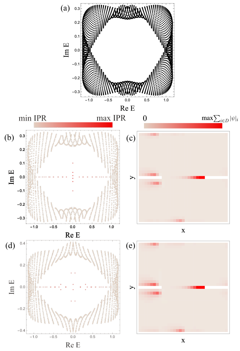
To strengthen our findings, we now turn our attention to class C. Consider the model
| (40) |
where is the two bands HN model defined in Eq. (36). and are the same as the previous section. This model obeys PHS with . It also obeys reflection symmetry in direction with such that . According to the classification Table 4 and 6, this model belongs to class C with symmetries, which possess a invariant.
In the sub-manifold , we have . Then we can define the winding number () for (), which lives in the () sector of reflection symmetry operator . Notice that since is a by matrix, . Then we see that . Hence, similar to model (35), mirror winding number (39) while the total winding number vanish. Thus, we see that the topological phase of model (40) is indeed protected by reflection symmetry.
We plot the spectrum of the model (40) in Fig. 5 (a) under full periodic boundary conditions (PBC). After the introduction of point defect, in-gap states that are localized around the defect begin to show (Fig. 5 (b) and (c)). Since the classification of class C without spatial symmetries is trivial in dimension (See Table 1), model (40) is another example of reflection-symmetry protected topological phases. We now try to break reflection symmetry while preserving PHS by introducing an on-site perturbation to the Hamiltonian. The resulting spectrum and localization of in-gap states are shown in Fig. 5 (d) and (e). Notably, instead of vanishing defect-localized in-gap states like class AI†, an imaginary-line gap is now open. The classification is now given by line gaps instead of point gaps. In this sense, the reflection symmetry is protecting point gaps for model (40).
VI.3 Point defect in D† with reflection symmetry
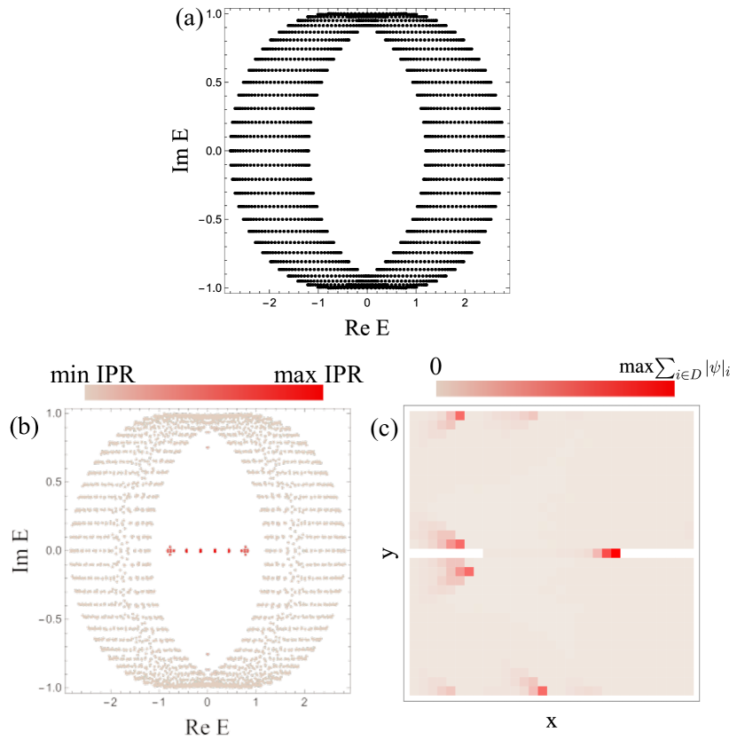
Now we introduce a model that is not protected by reflection symmetry. First notice, for class D† in dimension , it has the same topological invariant in the absence of spatial symmetry (Table 1) and with spatial symmetry in class (Table 6). We then consider the following model
| (41) |
where is two-bands HN model defined in Eq. (36); . This model obeys PHS† with . It also obeys the reflection symmetry in the direction with operator .
Unlike previous models (35) and (40), for model (41), defined on the sub-manifold for and have the same sign. More specifically, . Now, the mirror winding number (39) vanishes while the total winding number is nontrivial for . This shows that the topological phase of model (41) is not protected by reflection symmetry.
We plot its spectrum under full PBC in Fig. 6 (a). Similar to the previous two models, we introduce defects with Burgers vector . After the introduction of defects, as shown in Fig. 6 (b) and (c), we see that in-gap states that are localized around the defect appears. We now consider a reflection-symmetry-breaking term added to Hamiltonian. Since the topological invariant is not protected by reflection symmetry , we see that both point gap and localization of in-gap states are not affected by the introduction of additional term [Fig. 6 (d) and (e)].
VI.4 Point defect in DIII protected by reflection symmetry
Finally, we consider the following model
| (42) |
where , . Model (42) obeys TRS with , PHS with , and reflection symmetry in direction with . Since , , this place model (42) in class DIII with symmetry . According to Table 6, the model (42) has a invariant in the presence of a point defect. Furthermore, in the absence of spatial symmetries, class DIII has trivial classification for (Table 1).
We plot its spectrum under full PBC in Fig. 7 (a). Upon the introduction of point defects, in-gap states localized at the defects begin to appear [Fig. 7 (b) and (c)]. In-gap states are protected by a topological invariant. Notice that in the sub-manifold , reflection symmetry ensures that the coupling term would vanish. To see this, we consider the most general by Hamiltonian
| (43) |
The the reflection symmetry gives
| (44) |
Then we see that , which ensures that they must vanish at . In this sense, the reflection symmetry ensures that and are decoupled at . Return to model (42), we can define the topological invariant for each sector of defined for sub-manifold , where
| (45) |
where we also defined . A similar invariant can also be defined for Since the diagonal Hamiltonian and are decoupled at , even if they both have , the overall Hamiltonian is still topological.
To further confirm our claims that reflection symmetry protects topological invariant, we check the following two things: (i) By breaking reflection symmetries, the model (42) would either loss localization of in-gap states or open a line gap; (ii) To demonstrate the nature of this model, we stack two copies of (42) together with symmetry-preserving couplings. We expect the in-gap states would vanish in latter case. As we will see, these checking are indeed valid.
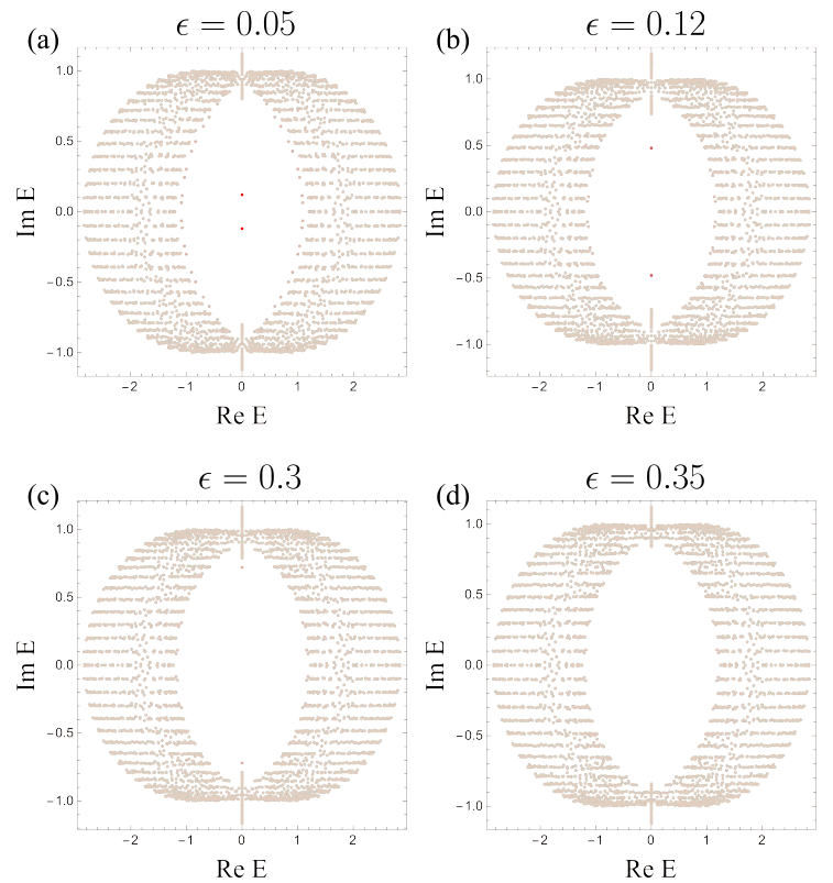
To confirm (i), we consider the introduction of a reflection-symmetry-breaking term . We first tune . As shown in Fig. 8 (a), there still exist two in-gap states. However, these two states are not topological. Indeed, increasing the strength of added term, we see that these two states shift into the bulk without closing the band gap of bulk bands [Fig. 8 (b)-(d)]. This means that these two states can be gaped out through continuous deformation. Hence, we see that the reflection symmetry is protecting the topological in-gap states.
To confirm (ii), we consider the stacked Hamiltonian
| (46) |
where the coupling is controlled by the parameter . The stacked Hamiltonian has all the symmetries that obeys. Although in-gap states exist for small value of , these states would merge into the bulk if we increase the value of without going through a phase transition (Fig. 9). Therefore, these states are not topological. Hence, we see that model (42) indeed has a invariant.
VII Discussions and Conclusions
In this paper, we give topological classification for all order-two spatial symmetries within AZ and AZ† class. The classification of crystalline symmetry for non-Hermitian system is a field that has been rarely studied. The classification table 6, 7, 8, 9 that we derived in the paper give a systematic way of understanding dislocation non-Hermitian skin effect proposed in [33, 34, 35]. In this paper, we generalized the classification results from Ref. [12] to non-Hermitian systems. Our classification is also more generalized than Ref. [47], which only considered reflection symmetry for non-Hermitian Hamiltonian without defects, and Ref. [48], which only considered defects with no spatial symmetries. Ref. [49] considered more generalized crystalline symmetries in non-Hermitian systems. However, Ref. [49] did not include internal symmetries in their classifications. In the grand scheme, our result paved the way for discovering novel symmetry-protected topological phases of non-Hermitian systems. As we have demonstrated in this paper, the existence of novel symmetry-protected topological phases also reveals that it is crucial to reexamine the effect of crystalline symmetries on non-Hermitian systems.
In this paper, we also demonstrate our findings through several toy models. Furthermore, we generalized the ”clock” shaped dimensional hierarchy of Hermitian Hamiltonian proposed in Ref. [10] to NH Hamiltonian within AZ and AZ† class. However, since AZ and AZ† constitute only out of -fold classification of NH matrices, it still remains a problem to find the classification for the rest of the classes. Since the -fold SLS classes are rarely studied in current literature, their classifications are left for future works.
Appendix A Dimensional Hierarchy of AZ and AZ† without spatial symmetries
| AZ class | Mapping | Type of | Mapped AZ class | TRS | PHS | CS |
| A | AIII | |||||
| AIII | A | |||||
| AI/AII | k | BDI/CII | ||||
| r | CI/DIII | |||||
| BDI/CII | k | D/C | ||||
| r | AI/AII | |||||
| D/C | k | DIII/CI | ||||
| r | BDI/CII | |||||
| DIII/CI | k | AII/AI | ||||
| r | D/C | |||||
| AZ† class | Mapped AZ† class | TRS† | PHS† | |||
| AI†/AII† | k | BDI†/CII† | ||||
| r | CI†/DIII† | |||||
| BDI†/CII† | k | D†/C† | ||||
| r | AI†/AII† | |||||
| D†/C† | k | DIII†/CI† | ||||
| r | BDI†/CII† | |||||
| DIII†/CI† | k | AII†/AI† | ||||
| r | D†/C† |
| AZ class | Symmetry | Type of | Mapped to | TRS | PHS | CS | Mapped symmetry | Mapped | |
|---|---|---|---|---|---|---|---|---|---|
| A | 0 | AIII | 0 | ||||||
| 1 | 1 | ||||||||
| 0 | 1 | ||||||||
| 1 | 0 | ||||||||
| AIII | 0 | A | 0 | ||||||
| 1 | 1 | ||||||||
| 0 | 1 | ||||||||
| 1 | 0 |
| AZ class | Symmetry | Type of | Mapped to | TRS | PHS | CS | Mapped symmetry | Mapped | |
|---|---|---|---|---|---|---|---|---|---|
| AI/AII | 0 | BDI/CII | 0 | ||||||
| 1 | 1 | ||||||||
| 2 | 2 | ||||||||
| 3 | 3 | ||||||||
| AI/AII | 0 | BDI/CII | 1 | ||||||
| 1 | 2 | ||||||||
| 2 | 3 | ||||||||
| 3 | 0 | ||||||||
| AI/AII | 0 | CI/DIII | 0 | ||||||
| 1 | 1 | ||||||||
| 2 | 2 | ||||||||
| 3 | 3 | ||||||||
| AI/AII | 0 | CI/DIII | 3 | ||||||
| 1 | 0 | ||||||||
| 2 | 1 | ||||||||
| 3 | 2 | ||||||||
| D/C | 0 | DIII/CI | 0 | ||||||
| 1 | 1 | ||||||||
| 2 | 2 | ||||||||
| 3 | 3 | ||||||||
| D/C | 0 | DIII/CI | 1 | ||||||
| 1 | 2 | ||||||||
| 2 | 3 | ||||||||
| 3 | 0 | ||||||||
| D/C | 0 | BDI/CII | 0 | ||||||
| 1 | 1 | ||||||||
| 2 | 2 | ||||||||
| 3 | 3 | ||||||||
| D/C | 0 | BDI/CII | 3 | ||||||
| 1 | 0 | ||||||||
| 2 | 1 | ||||||||
| 3 | 2 |
| AZ class | Symmetry | Type of | Mapped to | TRS | PHS | CS | Mapped symmetry | Mapped | |
|---|---|---|---|---|---|---|---|---|---|
| BDI/CII | 0 | D/C | 0 | ||||||
| 1 | 1 | ||||||||
| 2 | 2 | ||||||||
| 3 | 3 | ||||||||
| BDI/CII | 0 | D/C | 1 | ||||||
| 1 | 2 | ||||||||
| 2 | 3 | ||||||||
| 3 | 0 | ||||||||
| BDI/CII | 0 | AI/AII | 0 | ||||||
| 1 | 1 | ||||||||
| 2 | 2 | ||||||||
| 3 | 3 | ||||||||
| BDI/CII | 0 | AI/AII | 3 | ||||||
| 1 | 0 | ||||||||
| 2 | 1 | ||||||||
| 3 | 2 | ||||||||
| DIII/CI | 0 | AII/AI | 0 | ||||||
| 1 | 1 | ||||||||
| 2 | 2 | ||||||||
| 3 | 3 | ||||||||
| DIII/CI | 0 | AII/AI | 1 | ||||||
| 1 | 2 | ||||||||
| 2 | 3 | ||||||||
| 3 | 0 | ||||||||
| DIII/CI | 0 | D/C | 0 | ||||||
| 1 | 1 | ||||||||
| 2 | 2 | ||||||||
| 3 | 3 | ||||||||
| DIII/CI | 0 | D/C | 3 | ||||||
| 1 | 0 | ||||||||
| 2 | 1 | ||||||||
| 3 | 2 |
| AZ† class | Symmetry | Type of | Mapped to | TRS† | PHS† | CS | Mapped symmetry | Mapped | |
|---|---|---|---|---|---|---|---|---|---|
| AI†/AII† | 0 | BDI†/CII† | 0 | ||||||
| 1 | 1 | ||||||||
| 2 | 2 | ||||||||
| 3 | 3 | ||||||||
| AI†/AII† | 0 | BDI†/CII† | 3 | ||||||
| 1 | 0 | ||||||||
| 2 | 1 | ||||||||
| 3 | 2 | ||||||||
| AI†/AII† | 0 | CI†/DIII† | 0 | ||||||
| 1 | 1 | ||||||||
| 2 | 2 | ||||||||
| 3 | 3 | ||||||||
| AI†/AII† | 0 | CI†/DIII† | 1 | ||||||
| 1 | 2 | ||||||||
| 2 | 3 | ||||||||
| 3 | 0 | ||||||||
| D†/C† | 0 | DIII†/CI† | 0 | ||||||
| 1 | 1 | ||||||||
| 2 | 2 | ||||||||
| 3 | 3 | ||||||||
| D†/C† | 0 | DIII†/CI† | 3 | ||||||
| 1 | 0 | ||||||||
| 2 | 1 | ||||||||
| 3 | 2 | ||||||||
| D†/C† | 0 | BDI†/CII† | 0 | ||||||
| 1 | 1 | ||||||||
| 2 | 2 | ||||||||
| 3 | 3 | ||||||||
| D†/C† | 0 | BDI†/CII† | 1 | ||||||
| 1 | 2 | ||||||||
| 2 | 3 | ||||||||
| 3 | 0 |
| AZ† class | Symmetry | Type of | Mapped to | TRS† | PHS† | CS | Mapped symmetry | Mapped | |
|---|---|---|---|---|---|---|---|---|---|
| BDI†/CII† | 0 | D†/C† | 0 | ||||||
| 1 | 1 | ||||||||
| 2 | 2 | ||||||||
| 3 | 3 | ||||||||
| BDI†/CII† | 0 | D†/C† | 3 | ||||||
| 1 | 0 | ||||||||
| 2 | 1 | ||||||||
| 3 | 2 | ||||||||
| BDI†/CII† | 0 | AI†/AII† | 0 | ||||||
| 1 | 1 | ||||||||
| 2 | 2 | ||||||||
| 3 | 3 | ||||||||
| BDI†/CII† | 0 | AI†/AII† | 1 | ||||||
| 1 | 2 | ||||||||
| 2 | 3 | ||||||||
| 3 | 0 | ||||||||
| DIII†/CI† | 0 | AII†/AI† | 0 | ||||||
| 1 | 1 | ||||||||
| 2 | 2 | ||||||||
| 3 | 3 | ||||||||
| DIII†/CI† | 0 | AII†/AI† | 3 | ||||||
| 1 | 0 | ||||||||
| 2 | 1 | ||||||||
| 3 | 2 | ||||||||
| DIII†/CI† | 0 | D†/C† | 0 | ||||||
| 1 | 1 | ||||||||
| 2 | 2 | ||||||||
| 3 | 3 | ||||||||
| DIII†/CI† | 0 | D†/C† | 1 | ||||||
| 1 | 2 | ||||||||
| 2 | 3 | ||||||||
| 3 | 0 |
Similar to Hermitian case, we wish to derive a dimensional hierarchy for AZ and AZ† classes. In this section, we focus on the dimensional hierarchy for point-gapped Hamiltonian without any spatial symmetries. By dimensional hierachy, we mean the following relationship (isomorphism)
| (47) |
for complex AZ classes and
| (48) |
for real AZ classes and finally
| (49) |
for AZ† classes.
A.1 CS to non-CS classes
First we consider AZ class. We first consider a mapping that send a chiral symmetry Hamiltonian to a Hamiltonian without chiral symmetry .
Before discussing specific mappings, we specify the following requirements for the mappings. As mentioned in Sec. III, through continuous deformation, we can deform a point-gapped Hamiltonian into a unitary matrix , which obeys . The classification problem then becomes the classification of extended Hermitian Hamiltonian , which obeys [See Eq. (7)]. We introduce an extra dimension to which allows us to map the extended Hamiltonian to different symmetry classes. Let us call the mapping , which satisfy
| (50) |
The parameter can either be momentum-like or position-like. For a momentum-like (position-like) , it transforms the same way as k (r) under symmetries. In this case, the dimension of the Hamiltonian will increase (decrease) by [Recall that ].
We may write the mapping as
| (51) |
where is the term that would make the mapped Hamiltonian violate CS. Since is already in the form of an extended Hamiltonian, this further requires that is anti-diagonal and Hermitian. Finally, the condition requires that . Since the CS has the form , we see that by setting could satisfy all the conditions mentioned above. We thus define the following mapping
| (52) |
where . Notice that the mapping is defined for the extended Hermitian Hamiltonian (7). Due to the one to one relation between point-gapped Hamiltonian and its Hermitian extension, Eq. (52) is a valid mapping to send a chiral symmetric point-gapped Hamiltonian to a non-chiral one. Now, by varying types of between momentum-like or position-like, Eq. (52) provides a mapping between AZ classes with CS and without CS. In the following, we use some examples to illustrate this process.
For complex AZ class, notice that since there is no anti-unitary symmetries, we cannot distinguish momentum-like or position-like . Therefore, for both types of , Eq. (52) would send a Hamiltonian from class AIII () to class A ().
For real AZ classes with CS, both TRS and PHS symmetries may present. We make the requirement that . We may write the CS operator as
| (53) |
where is defined .
All the above derivations are also applicable to AZ† class. The mapping for AZ† class from a CS class to a non-CS one is the same as Eq. (52). However, the operator is now defined as
| (54) |
where we used the convention and is defined .
As an example, we consider is momentum-like. For AZ class, TRS is violated when while PHS is violated when . This corresponds to a clockwise rotation . Similarly, if is position-like, TRS is violated when . This corresponds to a counter-clockwise rotation . A similar conclusion also apply to AZ† class. All the mappings are summarized in Table 10.
To sum up this section, the mappings discussed above allow us to establish a one way mapping (homomorphism) from CS classes to non-CS classes i.e.
| (55) |
for complex AZ classes and
| (56) |
for real AZ classes and finally
| (57) |
for AZ† classes. In the next section, we consider one way mappings that would send a non-CS Hamiltonian to CS one such that the equal sign in Eq. (47) to (49) is justified.
A.2 Non-CS to CS classes
We focus on the mapping from non-CS to CS classes for AZ classes in this section ( to ). We first list the process of constructing mappings. Similar to the previous section, we introduce an extra dimension to such that the mapped Hamiltonian obeys CS. We define the mappings
| (58) |
where is or in a larger Clifford algebra dimension (See Table 10); is an extra term that made to obeys CS. Notice that unlike Eq. (52), the mapped Hamiltonian in Eq. (58) is not an extended Hamiltonian. Instead, is a point-gapped NH Hamiltonian that obeys unitary condition . Finally, we need to make sure that PHS and TRS of the mapped Hamiltonian commute with each other, as this is the convention we use in this papaer.
Bear these requirements in mind, we are now ready to discuss specific mappings.
First we consider a mapping from AI/AII to BDI/CII:
| (59) |
where obeys TRS with operator . If is a momentum-like parameter, the mapped Hamiltonian obeys TRS with ; PHS with . These two symmetries combined, obeys CS with . Furthermore, since the extended Hamiltonian obeys , we see that . This corresponds to a shift where (AI) or (AII).
Next, we consider a mapping that would map AI/AII to CI/DIII:
| (60) |
The is the symmetry operator of . If is position-like, the mapped Hamiltonian obeys TRS with and PHS with . Combining these two symmetries, obeys CS with . This corresponds to a shift where or .
By following similar process, we can find a mapping for class D/C and A into adjacent CS classes. For AZ† classes, the process of finding mappings into CS classes is essentially the same which we do not repeat here. The mapping and resulting symmetries are summarized in Table 10.
Appendix B Dimensional Hierarchy of AZ and AZ† with order-two spatial symmetries
In this section, we proof the dimensional hierarchy of AZ and AZ† in the presence of spatial symmetries.
B.1 Complex AZ with order-two unitary symmetries
Consider a Hamiltonian in class A with an additional symmetry . According to Table 2, this belongs to class . We consider the extended version on the mapped Hamiltonian in class AIII
| (64) |
as listed in Table 10. Once again, due to the absence of anti-unitary symmetries, we cannot distinguish whether is momentum-like or position-like. Therefore, we only need to consider whether will change under the spatial symmetries. If is i.e. unchanged under the spatial symmetries, we can define operator , since
| (65) |
Then the mapped Hamiltonian is now in . This process provide a homomorphism . Following similar process for other spatial symmetries, we arrive at Table 11, which allows us to conclude
| (66) |
This proof the relationship
| (67) |
B.2 Complex AZ with order-two anti-unitary symmetries
B.3 Real AZ and AZ† with order-two symmetries
We consider a Hamiltonian in class AI with symmetry . According to Table 4, this place the Hamiltonian in class . The mapping
| (68) |
provided in Table 10 allows to map to class BDI for a momentum-like . If the is not flipped under spatial symmetry i.e it is of the type , the mapped Hamiltonian obeys . This place in the class . Recall that in Sec. IV we showed that all anti-unitary spatial symmetries are equivalent to some of the unitary ones for real AZ classes (See Table 4). The process above then provide a homomorphsim . Following similar process for other spatial symmetries and AZ classes, we arrive at Table 12 and 13. These two tables allow us to conclude the relationships
| (69) |
which leads to
| (70) |
A similar analysis of AZ† classes with spatial symmetries results in Table 14 and 15, which allows us to conclude the relationship
| (71) |
Notice that for AZ† class, the effect of on is reversed [compare third and fifth row of Eqs. (69) and (71)]. Eq. (71) allows us to conclude
| (72) |
Appendix C Properties of Clifford Algebra
The complex Clifford algebras obeys
| (73) | ||||
| (74) | ||||
| (75) |
Notably, that represents complex matrices does not affect the extension problem. This means the extension problem is equivalent to the extension problem .
The real Clifford algebras obeys
| (76) | ||||
| (77) | ||||
| (78) | ||||
| (79) | ||||
| (80) | ||||
| (81) | ||||
| (82) | ||||
| (83) | ||||
| (84) |
where denotes the set of quaternions, denotes the real matrices. Similar to the previous case, does not affect the classification. This means extension problem is equivalent to the extension problem , and similar for to .
Appendix D Classifying space of AZ and AZ† with spatial symmetries from Clifford algebra
| Class | Symmetry | Generators | Extensions | Classifying space |
|---|---|---|---|---|
| A | ||||
| AIII | ||||
| AI | ||||
| BDI | ||||
| D | ||||
| DIII | ||||
| AII | ||||
| CII | ||||
| C | ||||
| CI | ||||
| AI† | ||||
| BDI† | ||||
| D† | ||||
| DIII† | ||||
| AII† | ||||
| CII† | ||||
|---|---|---|---|---|
| C† | ||||
| CI† | ||||
In this section, we introduce the process of finding the classifying space of Hamiltonians in AZ and AZ† class with additional spatial symmetries. The process is identical to Ref. [16, 12]. Since we have showed in Sec. IV that all antiunitary spatial symmetries can be mapped to unitary one, we only need to consider the addition of unitary symmetries to Hamiltonian.
D.1 Complex AZ classes
First we consider complex AZ classes. The complex Clifford algebra is generated by a set of generators , where all of the generators anti-commute with each other . Physically, these generators are symmetry operators of the Hamiltonian. The classification space can be found by the addition of extended Hamiltonian to the generators. Since the extended Hamiltonian obeys , we can put them into the generators without violating the properties of the set. The addition of Hamiltonian extends the generators by :
| (85) |
The mapping from provides us the classification space . Furthermore, obeys the so-called Bott periodicity . The Bott periodicity of complex Clifford algebra is the origin of two complex AZ classes. Hereafter, when referring to generator, we also include Hamiltonian.
The generators for point-gapped Hamiltonian with only internal symmetries (5) are provided in Ref. [37]. Notice that Ref. [37] used a different notation systems for symmetry classes from this paper and Kohei [24]. The relationship between these two different notation systems can be found in Ref. [48].
The addition of spatial symmetries would change the classification of original classes. To see this, let’s consider a order-two spatial symmetry is added to the classification. There are two possible ways in which the addition of changes the classification.
(1) Through combination of with other generators, the resulting generator might anti-commute with all other generators i.e. for all and . In such a case, the generators would become . Correspondingly, the classifying space would shift by .
(2) It is also possible that commutes with all other generators i.e. for all and . The generators then become . In this case, the Hilbert space splits into two eigenspaces of . Each eigenspace has the same Clifford algebra and hence the same classifying space. The classifying space then becomes .
As an example, consider a point-gapped Hamiltonian in class A. The only symmetry obeys in this class is the symmetry [Eq. (9)]. Therefore, the Hamiltonian extends the generators as
| (86) |
which has classification space . This is the classification of class A given in Table 1. Next, consider the addition of spatial symmetry to the system. Recall that anti-commutes with . Then the operator anti-commutes with both and . Now, the generators are given by
| (87) |
which has classifying space .
As another example, we consider a point-gapped Hamiltonian in class A with the addition of . Recall that the extended operator that acts on extended Hamiltonian commutes with both and . Therefore, the generators are now given by
| (88) |
which has classifying space .
Following a similar process, we summarize the classification of complex AZ classes under spatial symmetries in the first two rows of Table 16.
D.2 Real AZ and AZ† classes
Now consider real AZ and AZ† classes. Their classifying space are given by the real Clifford algebra , where , for and for . In this case, the Hamiltonian can extend the generators by
| (89) |
In this case, the classifying space is given by . Hamiltonian can also extend the generators by
| (90) |
The classifying space is given by .
Now let’s consider the addition of order-two spatial symmetry . Similar to complex AZ classes, through the combination of and other generators as well as the imaginary unit , the resulting generator would commute or anti-commute with the rest of the generators. However, due to the presence of antiunitary symmetries, we need to consider the squared value of . Since , we have four possible situations.
(1) anti-commutes with all generators and . In this case the generators would change by . The new classifying space would be () if ()
(2) anti-commutes with all generators and . In this case the generators would change by . The new classifying space would be () if ()
(3) commutes with all generators and . In this case, would introduce complex structure to real Clifford algebra. The set of generators without Hamiltonian is written as . Thus, the classifying space would be the same as complex AZ classes. In fact, we have the relationship (Appendix C). The classifying space is then given by .
(4) commutes with all generators and . In this case, the Hilbert space splits into two eigenspace of . The classifying space is given by () if ().
As an example, we consider the classification of class AI in addition to . The generators for point-gapped AI class is given by [37]
| (91) |
where is the TRS operator and is the symmetry (9). Since , the extension is which gives classifying space . Now we consider the addition of spatial symmetry . Notice that anti-commutes with all the generators in Eq. (91) and it squares to (Recall that and anti-commute). Therefore, the new set of generators is
| (92) |
The extension is now given by , which gives classifying space .
Following these procedures, we arrive at Table 16 for real AZ and AZ† classes.
References
- Qi and Zhang [2011] X.-L. Qi and S.-C. Zhang, Topological insulators and superconductors, Rev. Mod. Phys. 83, 1057 (2011).
- Hasan and Kane [2010] M. Z. Hasan and C. L. Kane, Colloquium: Topological insulators, Rev. Mod. Phys. 82, 3045 (2010).
- Moore [2010] J. E. Moore, The birth of topological insulators, Nature 464, 194–198 (2010).
- Sato and Ando [2017] M. Sato and Y. Ando, Topological superconductors: a review, Reports on Progress in Physics 80, 076501 (2017).
- Kitaev et al. [2009] A. Kitaev, V. Lebedev, and M. Feigel’man, Periodic table for topological insulators and superconductors, AIP Conference Proceedings 10.1063/1.3149495 (2009).
- Altland and Zirnbauer [1997] A. Altland and M. R. Zirnbauer, Nonstandard symmetry classes in mesoscopic normal-superconducting hybrid structures, Phys. Rev. B 55, 1142 (1997).
- Chiu et al. [2016] C.-K. Chiu, J. C. Y. Teo, A. P. Schnyder, and S. Ryu, Classification of topological quantum matter with symmetries, Rev. Mod. Phys. 88, 035005 (2016).
- Kane and Mele [2005a] C. L. Kane and E. J. Mele, topological order and the quantum spin hall effect, Phys. Rev. Lett. 95, 146802 (2005a).
- Kane and Mele [2005b] C. L. Kane and E. J. Mele, Quantum spin hall effect in graphene, Phys. Rev. Lett. 95, 226801 (2005b).
- Teo and Kane [2010] J. C. Y. Teo and C. L. Kane, Topological defects and gapless modes in insulators and superconductors, Phys. Rev. B 82, 115120 (2010).
- Teo and Hughes [2017] J. C. Teo and T. L. Hughes, Topological defects in symmetry-protected topological phases, Annual Review of Condensed Matter Physics 8, 211–237 (2017).
- Shiozaki and Sato [2014] K. Shiozaki and M. Sato, Topology of crystalline insulators and superconductors, Phys. Rev. B 90, 165114 (2014).
- Fu and Kane [2007] L. Fu and C. L. Kane, Topological insulators with inversion symmetry, Phys. Rev. B 76, 045302 (2007).
- Fu [2011] L. Fu, Topological crystalline insulators, Phys. Rev. Lett. 106, 106802 (2011).
- Chiu et al. [2013] C.-K. Chiu, H. Yao, and S. Ryu, Classification of topological insulators and superconductors in the presence of reflection symmetry, Phys. Rev. B 88, 075142 (2013).
- Morimoto and Furusaki [2013] T. Morimoto and A. Furusaki, Topological classification with additional symmetries from clifford algebras, Phys. Rev. B 88, 125129 (2013).
- Shiozaki et al. [2016] K. Shiozaki, M. Sato, and K. Gomi, Topology of nonsymmorphic crystalline insulators and superconductors, Phys. Rev. B 93, 195413 (2016).
- Shiozaki et al. [2017] K. Shiozaki, M. Sato, and K. Gomi, Topological crystalline materials: General formulation, module structure, and wallpaper groups, Phys. Rev. B 95, 235425 (2017).
- Cano et al. [2018] J. Cano, B. Bradlyn, Z. Wang, L. Elcoro, M. G. Vergniory, C. Felser, M. I. Aroyo, and B. A. Bernevig, Building blocks of topological quantum chemistry: Elementary band representations, Phys. Rev. B 97, 035139 (2018).
- Bradlyn et al. [2017] B. Bradlyn, L. Elcoro, J. Cano, M. G. Vergniory, Z. Wang, C. Felser, M. I. Aroyo, and B. A. Bernevig, Topological quantum chemistry, Nature 547, 298–305 (2017).
- Yao and Wang [2018] S. Yao and Z. Wang, Edge states and topological invariants of non-hermitian systems, Phys. Rev. Lett. 121, 086803 (2018).
- Song et al. [2019] F. Song, S. Yao, and Z. Wang, Non-hermitian skin effect and chiral damping in open quantum systems, Phys. Rev. Lett. 123, 170401 (2019).
- Okuma et al. [2020] N. Okuma, K. Kawabata, K. Shiozaki, and M. Sato, Topological origin of non-hermitian skin effects, Phys. Rev. Lett. 124, 086801 (2020).
- Kawabata et al. [2019a] K. Kawabata, K. Shiozaki, M. Ueda, and M. Sato, Symmetry and topology in non-hermitian physics, Phys. Rev. X 9, 041015 (2019a).
- Xiujuan Zhang and Chen [2022] M.-H. L. Xiujuan Zhang, Tian Zhang and Y.-F. Chen, A review on non-hermitian skin effect, Advances in Physics: X 7, 2109431 (2022), https://doi.org/10.1080/23746149.2022.2109431 .
- Zhang et al. [2022] K. Zhang, Z. Yang, and C. Fang, Universal non-hermitian skin effect in two and higher dimensions, Nature Communications 13, 10.1038/s41467-022-30161-6 (2022).
- Lin et al. [2023] R. Lin, T. Tai, L. Li, and C. H. Lee, Topological non-hermitian skin effect, Frontiers of Physics 18, 10.1007/s11467-023-1309-z (2023).
- Okugawa et al. [2020] R. Okugawa, R. Takahashi, and K. Yokomizo, Second-order topological non-hermitian skin effects, Phys. Rev. B 102, 241202 (2020).
- Kawabata et al. [2020] K. Kawabata, M. Sato, and K. Shiozaki, Higher-order non-hermitian skin effect, Phys. Rev. B 102, 205118 (2020).
- Liu et al. [2019a] T. Liu, Y.-R. Zhang, Q. Ai, Z. Gong, K. Kawabata, M. Ueda, and F. Nori, Second-order topological phases in non-hermitian systems, Phys. Rev. Lett. 122, 076801 (2019a).
- Zhang et al. [2020] K. Zhang, Z. Yang, and C. Fang, Correspondence between winding numbers and skin modes in non-hermitian systems, Phys. Rev. Lett. 125, 126402 (2020).
- Yang et al. [2020] Z. Yang, K. Zhang, C. Fang, and J. Hu, Non-hermitian bulk-boundary correspondence and auxiliary generalized brillouin zone theory, Phys. Rev. Lett. 125, 226402 (2020).
- Schindler and Prem [2021] F. Schindler and A. Prem, Dislocation non-hermitian skin effect, Phys. Rev. B 104, L161106 (2021).
- Bhargava et al. [2021] B. A. Bhargava, I. C. Fulga, J. van den Brink, and A. G. Moghaddam, Non-hermitian skin effect of dislocations and its topological origin, Phys. Rev. B 104, L241402 (2021).
- Panigrahi et al. [2022] A. Panigrahi, R. Moessner, and B. Roy, Non-hermitian dislocation modes: Stability and melting across exceptional points, Phys. Rev. B 106, L041302 (2022).
- Ammari et al. [2024] H. Ammari, S. Barandun, J. Cao, B. Davies, and E. O. Hiltunen, Mathematical foundations of the non-hermitian skin effect, Archive for Rational Mechanics and Analysis 248, 10.1007/s00205-024-01976-y (2024).
- Zhou and Lee [2019] H. Zhou and J. Y. Lee, Periodic table for topological bands with non-hermitian symmetries, Phys. Rev. B 99, 235112 (2019).
- Ahn et al. [2019] J. Ahn, S. Park, and B.-J. Yang, Failure of nielsen-ninomiya theorem and fragile topology in two-dimensional systems with space-time inversion symmetry: Application to twisted bilayer graphene at magic angle, Phys. Rev. X 9, 021013 (2019).
- Hwang et al. [2019] Y. Hwang, J. Ahn, and B.-J. Yang, Fragile topology protected by inversion symmetry: Diagnosis, bulk-boundary correspondence, and wilson loop, Phys. Rev. B 100, 205126 (2019).
- Song et al. [2020] Z.-D. Song, L. Elcoro, and B. A. Bernevig, Twisted bulk-boundary correspondence of fragile topology, Science 367, 794 (2020), https://www.science.org/doi/pdf/10.1126/science.aaz7650 .
- Po et al. [2018] H. C. Po, H. Watanabe, and A. Vishwanath, Fragile topology and wannier obstructions, Phys. Rev. Lett. 121, 126402 (2018).
- Brouwer and Dwivedi [2023] P. W. Brouwer and V. Dwivedi, Homotopic classification of band structures: Stable, fragile, delicate, and stable representation-protected topology, Phys. Rev. B 108, 155137 (2023).
- Moore et al. [2008] J. E. Moore, Y. Ran, and X.-G. Wen, Topological surface states in three-dimensional magnetic insulators, Phys. Rev. Lett. 101, 186805 (2008).
- Kawabata et al. [2019b] K. Kawabata, S. Higashikawa, Z. Gong, Y. Ashida, and M. Ueda, Topological unification of time-reversal and particle-hole symmetries in non-hermitian physics, Nature Communications 10, 10.1038/s41467-018-08254-y (2019b).
- Roy and Harper [2017] R. Roy and F. Harper, Periodic table for floquet topological insulators, Phys. Rev. B 96, 155118 (2017).
- Yoshida et al. [2020] T. Yoshida, T. Mizoguchi, and Y. Hatsugai, Mirror skin effect and its electric circuit simulation, Phys. Rev. Res. 2, 022062 (2020).
- Liu et al. [2019b] C.-H. Liu, H. Jiang, and S. Chen, Topological classification of non-hermitian systems with reflection symmetry, Phys. Rev. B 99, 125103 (2019b).
- Liu and Chen [2019] C.-H. Liu and S. Chen, Topological classification of defects in non-hermitian systems, Phys. Rev. B 100, 144106 (2019).
- Shiozaki and Ono [2021] K. Shiozaki and S. Ono, Symmetry indicator in non-hermitian systems, Phys. Rev. B 104, 035424 (2021).