Variational Pattern Selection

Abstract

We address pattern selection problems in nonlinear interface dynamics by maximizing the entropy of the most probable (classical) scenario associated with the processes. This variational principle we applied to well-known selection problems in a Hele-Shaw cell: stationary Saffman-Taylor finger in a channel [1] and self-similar finger in a wedge [2]. The obtained results excellently agree with experiments. We also address the universal fjord opening angle [3]. This principle complements a non-variational selection developed earlier [4]. Surface tension is not needed for selection in both approaches, contrary to the common belief.

I Introduction

Selection problems. Of the many unstable nonlinear phenomena, we will address here only those describing front propagation, pattern formation, and self-organization. Besides being of obvious interests for mathematics, physics, geophysics, chemistry, and biology, they are indispensable in oil/gas recovery, metallurgy, and medicine (malignant growth), to name just a few applications. These processes often exhibit the problem of selecting the most stable member from a family of stationary or self-similar solutions.

List of pioneers. The first work in this subject was in gene propagation (Kolmogorov et al. [5]). Based on citations, selections of fluid/fluid interfaces named after Taylor (Rayleigh-Taylor [6] and Saffman-Taylor [1] instabilities) attracted most of attention. Comparable efforts were also in calculating of asymptotic velocities in flame propagation (Landau [7], Zeldovich [8], Gelfand [9]), crack propagation (Mott [10], Barenblatt [11]), and dendritic growth (Ivantsov [12], Langer [13]). These impressive names reflect both importance and difficulty of selection problems.

Extremum principle. Selection problems are challenging both in physics (to identify the selection mechanism) and in mathematics (to handle a small singular term). The desire to find a functional, whose extremal describes the selected pattern, is understandable. But since all these processes are out of equilibrium, minimizing thermodynamic potentials here is out of help. Importance of the extremum principle was clearly indicated by one of pioneers in dendritic growth selection, J. S. Langer: After noticing “[t]he big, unsolved part of the problem is how these complex shapes are selected”, he asks: “…might there be some meaningful and useful variational formulation that describes these processes?” [13].

Minimal dissipation is out of help. There is one such functional applicable out of equilibrium – the principle of minimal dissipation in viscous hydrodynamics, discovered by Helmholtz and Korteveg in XIX century (see [14]), and also valid in kinetics of weakly non-equilibrium systems, as discovered by Onsager in 1931 [15]. In fact, the authors of [1] tried to apply this functional to select the observed inviscid finger with a relative width of 1/2 in a Hele-Shaw cell. However, it turned out that complete dissipation (friction between plates and oil) does not depend on the finger shape at all, and thus is out of help. This was one of motivations to include surface tension as the largest factor neglected in deriving a continuum family of stationary fingers (see Section II below), for solving the selection problem.

Goals of the paper. Being mostly dissipative, these processes do not possess the action, which minimum provides their dynamics in the form of Euler-Lagrange equations. Earlier we developed a stochastic theory [16, 17], where we obtained dissipative deterministic growth equations by varying an entropy associated with stochastic processes. In this article, we maximize the entropy for deterministic processes to address well-known selection problems in a Hele-Shaw cell. The obtained results excellently agree with experiments and do not require surface tension, contrary to common belief.

Structure of the paper. There are two sections, which follow the introduction. The first one contains a background of non-variational approaches to selection both with and without surface tension. Then the second section follows, which is fully devoted to the variational approach, where our stochastic theory and a variational principle are presented and applied to three selections in a Hele-Shaw cell: a finger in a channel [1], a finger in a wedge [2], and a fjord angle [3]. A conclusion is stated at the end of the article.

II Non-variational approaches to selection

II.1 Selection via surface tension

Problems with including surface tension. To see how surface tension explains the Saffman-Taylor finger (STF) selection, one has to include the surface tension term into the equation for a family of steady state solutions written in scaled units as $x=Ut+2(1-\lambda)\log(\cos(y/2\lambda))$ [1]. Here $x$ and $y$ are Cartesian coordinates in a physical plane, $x(t,y)$ is a moving interface parameterized by $y$, $t$ is time, and $\lambda$ is a ratio of the finger width to the lateral width of a Hele-Shaw channel. The task is to select $\lambda=1/2$ from the continuum, $0<\lambda<1$, as the most stable member of this family by including surface tension. But inclusion of surface tension is non-trivial, because the term with surface tension provides a singular perturbation. In other words this term, added to the equation of motion (eq. (7) below) presents the highest spatial derivative multiplied by a small number (surface tension), thus all regular perturbative corrections are zero. So including surface tension for solving selection problem appeared as a problem by itself.

WKB. This singular perturbation problem was solved by using the WKB approximation developed in 1926 in quasi-classical quantum mechanics [18], because of the striking similarity between the surface tension term and a square of the (small) Planck constant, $\hbar$, multiplied by the highest (second) derivative in the Schrödinger equation. This method, based on analytic continuation into a complex plane, helped to answer many questions in quantum mechanics, such as quantum tunneling, Bohr-Sommerfeld quantization, and presenting the action as an adiabatic invariant. The WKB-based analytic continuation approach (the so-called “Zwaan method” [19]) was resurrected in 1961 by Pokrovsky and Khalatnikov working on the over-barrier reflection [20].

Selection problem solved. To adapt WKB to selection problems Kruskal and Segur developed a theory of “Asymptotic beyond all orders” [21]. This theory allowed one to catch exponentially small terms after analytic continuation from the real axis to a complex plane, and so to find a discrete spectrum of branches converging to $\lambda=1/2$ in zero surface tension limit. Then it was demonstrated with computational help that the lowest branch is the most stable one. These results were culminated in 1986 when several independent groups simultaneously reported in (the same issue of) PRL [22, 23, 24] the successful completion of the STF selection problem. These achievements were summarized and presented in various books and reviews [25, 26, 27, 28].

II.2 Selection without surface tension

Integrability. However, it was shown in 1998 that STF selection does not require surface tension [4], [29]. The result [4] was achieved due to integrability of the Laplacian growth (LG) [30], that is the interface dynamics in a Hele-Shaw cell without surface tension. This remarkable property, which allows to obtain various classes of exact unsteady solutions, is rather an exception than a rule among nonlinear PDEs or other infinitely dimensional dynamical systems. Integrability, as a new branch of mathematical physics, was born in 1967 after the discovery of striking and unusual (at that time) properties of the Korteveg de Vries equation [31]. This field has been booming since then with no signs of slowing down up to date.

Hadamard ill-posedness. LG is linearly unstable, and all exact unsteady solutions of LG are either singular, i.e., cease to exist in a finite time [32, 33, 34], or regular, i.e., exist at all times and therefore allow analysis in long-term asymptotics, $t\to\infty$ [35, 36, 37, 38, 39]. Because of instability and divergent solutions, the LG equation is ill-posed in the Hadamard sense [40], which is typical for many important equations correctly describing physical processes [41]. In the 1960s, Hadamard’s counterexample, which gave birth to the whole concept of ill-posed problems, was found to be wrong [42]. But reluctance of mathematicians to take seriously such ill-posed equations, instead of claiming them meaningless, slowed down progress in certain areas of physics in 1920-1950s [43] by delaying important development in these fields.

Tikhonov regularization. Converting ill-posed (in the Hadamard sense) equations into well-posed ones was developed in 1950-1960s in USSR and based on these efforts a rigorous theory was created by Tikhonov [44] and named after him. This procedure eliminates all initial data leading to singular solutions as unphysical and non-observable. If all the initial interfaces can be approximated as closely as desired by the data remaining after elimination, then the problem is proven to be well-posed, and these data are called the set of well-posedness [45].

External and internal regularizations. Unlike widely used ”external” regularizations when small dispersive terms are added to ill-posed equations (such as surface tension regularization discussed above), a less conventional Tikhonov procedure of eliminating all initial data leading to divergent solutions, is the ”internal” one. Sometimes internal regularization is more advantageous than external one. It is clearly the case for Laplacian growth, which subtle integrable structure retains intact after Tikhonov regularization, but is totally ruined by including surface tension. Selection without surface tension in [4] was performed precisely by this procedure, which converted the problem into a well-posed one.

Bubble selection. The approach developed in [4] for finger selection without surface tension was later applied to bubble selection in a channel [46, 47, 48, 49]. In [46, 48] the authors obtained new classes of exact unsteady solutions for a bubble with an arbitrary shape. By applying these solutions to the single bubble selection problem, posed in [50], they reproduced the selected value obtained by including surface tension and then applying asymptotics beyond all orders mentioned above [51]. Recently asymptotic velocity selection was predicted for an arbitrary number of nonlinearly interacted bubbles in a channel [49].

The only attractor. The key observation common to all these works is that the observed pattern selected from continuum is the only attractor of (and, as such, is built in) zero surface tension dynamics. These results became possible due to a rich set of exact unsteady regular solutions of LG because of its integrable structure as well as due to the Tikhonov regularization, which converted the ill-posed problem to the well-posed one.

These selections came from differential equations, but not from variation of a functional, so Langer’s question in [13] about variational formulation still persists. After applying the entropy functional defined below to the Saffman-Taylor selection problems in the next section, we believe the answer is “yes”.

III Variational selection

III.1 Stochastic growth theory

Stochastic growth in a nutshell. Assume $K$ tiny Brownian particles of the area $\hbar$, issued from infinity and land on a boundary $\partial D(t)$ of a growing domain $D(t)$ [16, 17] within each time unit. This process is a bridge (crossover) between $K=1$, describing DLA process [52], and $K\to\infty$, $\hbar\to 0$, which corresponds to a deterministic Laplacian growth (LG) described by the bilinear equation (7) below. $K=1$ is a quantum limit because of the maximal correlation between Brownian particles, while $K\to\infty$ is a classical limit since all $K$ issued particles are independent (fully uncorrelated). The correspondence with the classical limit requires the condition

$$K\hbar=Q\delta t.$$ (1)

This is the area of a (thin) layer, $\delta D(t)$, attached to the domain $D(t)$ during a (small) time interval $\delta t$, and $Q$ is a strength of a fluid source in a deterministic Laplacian growth.

Multinomial stochasticity. Let’s partition the boundary $\partial D(t)$ onto $N\gg 1$ equal fragments (bins) and define $\mu_{i}$ to be a probability of a single particle to land to $i$-th fragment (bin), hence the constraint

$$\sum_{i=1}^{N}\mu_{i}=1.$$ (2)

For LG $\mu_{i}$ is a harmonic measure [53] of the $i$-th fragment of a boundary, which equals

$$\mu_{i}=-\frac{\partial_{n}G(\xi_{i},\infty)}{2\pi}|d\xi_{i}|.$$ (3)

Here $G(\xi_{i},\infty)$ is the Green function of the Laplace operator, defined as a function harmonic outside a growing pattern, diverging logarithmically at $\infty$, and vanishing at the boundary, $\partial D(t)$; $\xi_{i}$ here is (any) point of the $i^{th}$ bin, introduced above.

The statistical weight that $k_{i}$ particles lands to the $i$-th bin ($i=1,2,\dotsc,N$) within a (small) time unit, $\delta t$, is given by the multinomial distribution:

$$P(k_{1},\dotsc,k_{N})=K^{N}\prod_{i=1}^{N}\frac{\mu_{i}^{k_{i}}}{k_{i}!},$$ (4)

which after the Stirling approximation, by assuming $k_{i}\gg 1$, amounts to

$$P(k_{1},\dotsc,k_{N})=\exp\Bigl{\{}K\log K\Bigr{.}\\ \Bigl{.}-\sum_{i=1}^{N}k_{i}\log(k_{i}/(\mu_{i}K)\Bigr{\}}=\exp S[\delta D(t)],$$ (5)

where $S[\delta D(t)]$ is the entropy of the layer, $\delta D(t)$.

Maximal (classical) entropy. By varying this entropy functional with respect to a stochastic $k_{i}$, subject to the constraint (2), we find that $S[\delta D(t)]$ reaches the maximum when

$$\bar{k}_{i}=K\mu_{i}.$$ (6)

By equating a small displacement of the $i$-th fragment of a boundary, $V_{n}(\xi_{i})\,\delta t$, where $V_{n}(\xi_{i})$ is a normal interface velocity at the point $\xi_{i}$, to $\bar{k}_{i}=K\mu_{i}$, we immediately derive the deterministic (classical) equation of growth, as the Euler-Lagrange equation of motion, or in other words the extremal of the action equaled to a negative entropy, $-S[\delta D(t)]$. For the Laplacian growth this equation takes a form

$${\mathcal{I}}\text{m}\left(\bar{z}_{t}z_{\phi}\right)=\frac{Q}{2\pi},$$ (7)

where $z(t,w)$ is the conformal map from the exterior of the unit circle on the $w$-plane to the domain $D(t)$ on the physical $z$-plane, where $z=x+iy$; the boundary of $D(t)$ is $z(t,\exp(i\phi))$ parametrized by $\phi\in[0,2\pi]$, and subscripts denote partial derivatives. We skip a simple derivation of (7) from (6) by using (1) (see [16, 17]) for want of space.

Rich structure. The negative entropy in (5) after simple transformations becomes the action with a symplectic structure and the Hamilton-Jacobi formalism. Besides (and quite surprisingly), eq. (7) is equivalent to the classical Hadamard formula for a change of the Green function $G(\xi,\infty)$ after variation of $D(t)$ [54]. (More information about this remarkable structure underlying the eq. (7) and its relations to 2D quantum gravity, quantum Hall phenomena, random matrices, and integrable hierarchies can be found in  [30, 55, 56, 57].)

Entropy = Scaled area. Bearing in mind that $K\hbar$ is the area of a single layer of growth, we obtain after plugging (6) into (5), the maximal (deterministic) entropy for a process, described by (6), in a strikingly simple form:

$$S[D(T)]=K(T/\delta t)\log N=C\cdot\text{Area}[D(T)],$$ (8)

where $K$ is the same for each time interval $\delta t$, $T$ is a total time of growth, so $K(T/\delta t)\hbar$ is the area spanned by the growing pattern during time $T$, and $C=\log N/\hbar$.

Variational selection. Since Nature always favors the largest entropy scenario, then in view of (8) to solve the selection problem is to find a value of a parameter to select from (it is $\lambda$ in the STF case), which maximizes the area spanned by the growing domain $D(t)$.

III.2 Selection in a channel

We cannot apply the maximal area principle to the family of the Saffman-Taylor fingers

$$x=Ut+2(1-\lambda)\log(\cos(y/2\lambda)),$$ (9)

since they are infinitely long, so their interior area diverges.

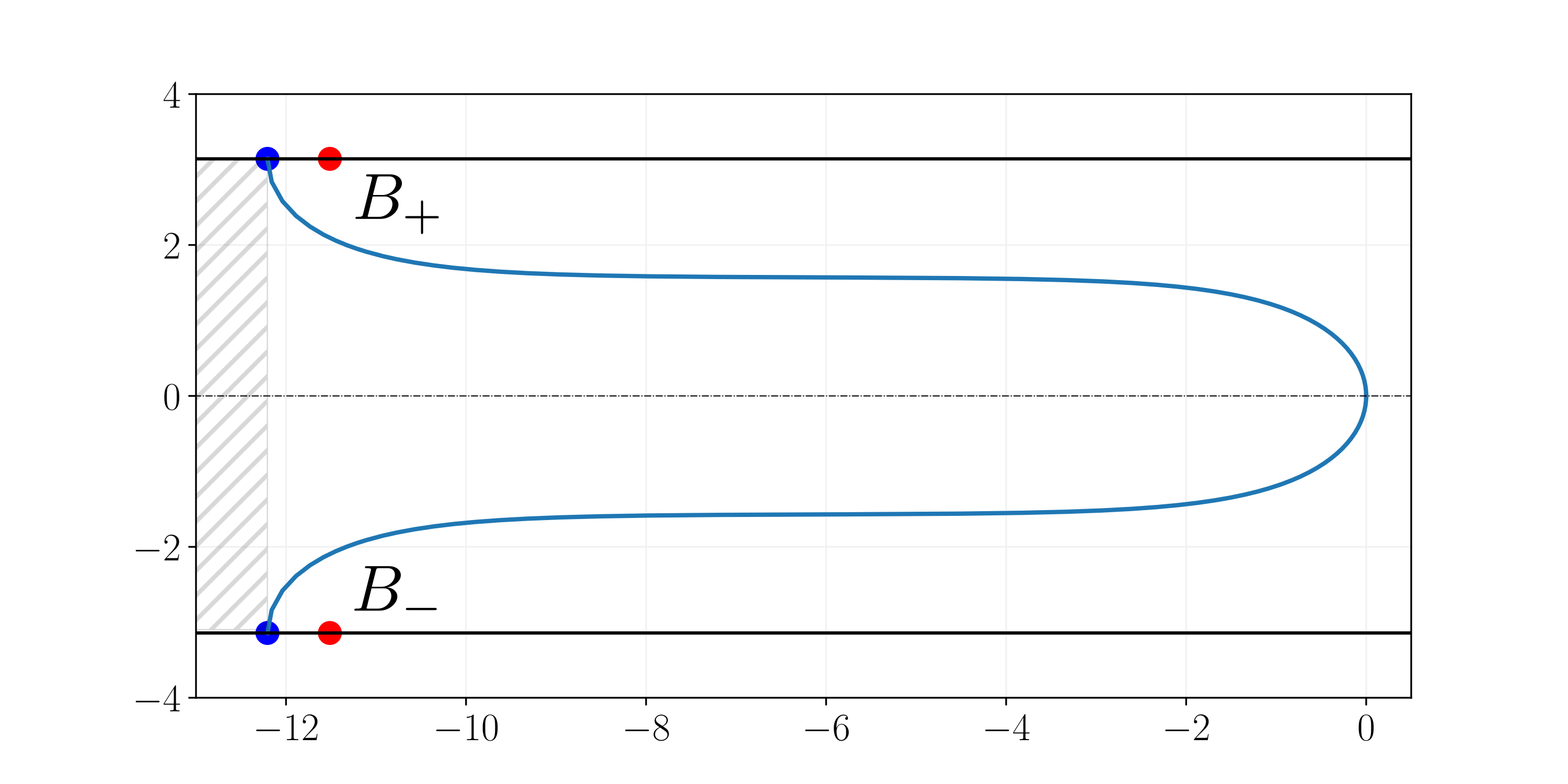
Figure 1: Moving finger in a rectangular channel, described by eq. (9). Constants of motion, $B_{\pm}=B\pm i\pi$ are indicated by little red circles at the channel’s walls. The stagnation points, the interface moves to exponentially slow, equal, $B_{\pm}-2(1-\lambda)\log 2$, are also located at the walls (little blue circles). The dashed rectangle is the unphysical part of the total finger area.

Fortunately, there is an unsteady solution for a finite finger [58, 37, 38, 39, 4] shown in Fig. 1:

$$z=r(t)+i\phi+2(1-\lambda)\log(1-a(t)\exp(-i\phi)),$$ (10)

where $r(t)$ and $a(t)$ can be found from the following two equations:

$$\begin{gathered}{\mathcal{A}}=t=r(t)+2(1-\lambda)^{2}\log(1-a(t)^{2}),\\ B=z(t,1/a(t))=r(t)+2(1-\lambda)\log(1-a(t)^{2}),\end{gathered}$$ (11)

where ${\mathcal{A}}$ is the area inside the finger, which equals time, $t$, in our scaled units, $Q=2\pi$, in (7). $B$ is a constant of motion, as follows from (7), and stems from integrability of the system, but more precisely from the Herglotz theorem on singularity correspondence [59, 60, 16, 17]; $r(t)$ is the moving fingertip, and $a(t)$ relates to a finger length, $2(1-\lambda)^{2}\log[1/(1-a(t)^{2})]$, which diverges when $a(t)\to 1$. Initially, at $t=0$, the finger is almost flat, so $a(0)\ll 1$. Then $a$ starts to grow and because $da(t)/dt>0$ it moves (exponentially slow when $t\to\infty$) toward 1.

After eliminating $r(t)$ in these two equations by subtracting $B$ from ${\mathcal{A}}$ in (11), we obtain:

$${\mathcal{A}}(\lambda,a(t))=B+2\lambda(1-\lambda)\log\frac{1}{1-a(t)^{2}}.$$ (12)

Geometrically this subtraction is a removal of the unphysical part of the total finger area, that is the rectangle, shown in Fig. 1. Prior the interface reaches a stagnation point, $B-2(1-\lambda)^{2}\log 2$, at the walls, there is a nonlinear competition of different fingers until the survival of the leading one [39, 4]. The point of intersection of the interface with walls gradually slows down and finally stops at (speaking strictly, it continues to move exponentially slow to) the stagnation point. This completes formation of the finger, which propagates since then without deformation.

As the eq. (12) shows, the area, ${\mathcal{A}}(\lambda,a(t))$, is maximal at $\lambda=1/2$, which is the selected value in accordance with the classical experiment [1]. This selection is achieved by a simple variational principle, which favors the most probable scenario (see above) and amounts to the maximal area spanned by the evolving pattern. This variational principle is the second selection without surface tension, complementing the dynamical selection with the same result obtained earlier [4] from the exact unsteady solutions of the regularized eq. (7).

III.3 Selection in a wedge

Formulations of a selection problem in rectangular and wedge geometries are quite similar: to select the observable (and thus the most stable) member of the continuum of self-similar solutions for a finger in a wedge. These solutions are labeled by the wedge angle, $\theta=\pi\kappa$, and by the angle, $\alpha=\pi(\kappa-\beta)$, between two tangents to the finger at the wedge apex. The parameter of selection is ratio of these angles

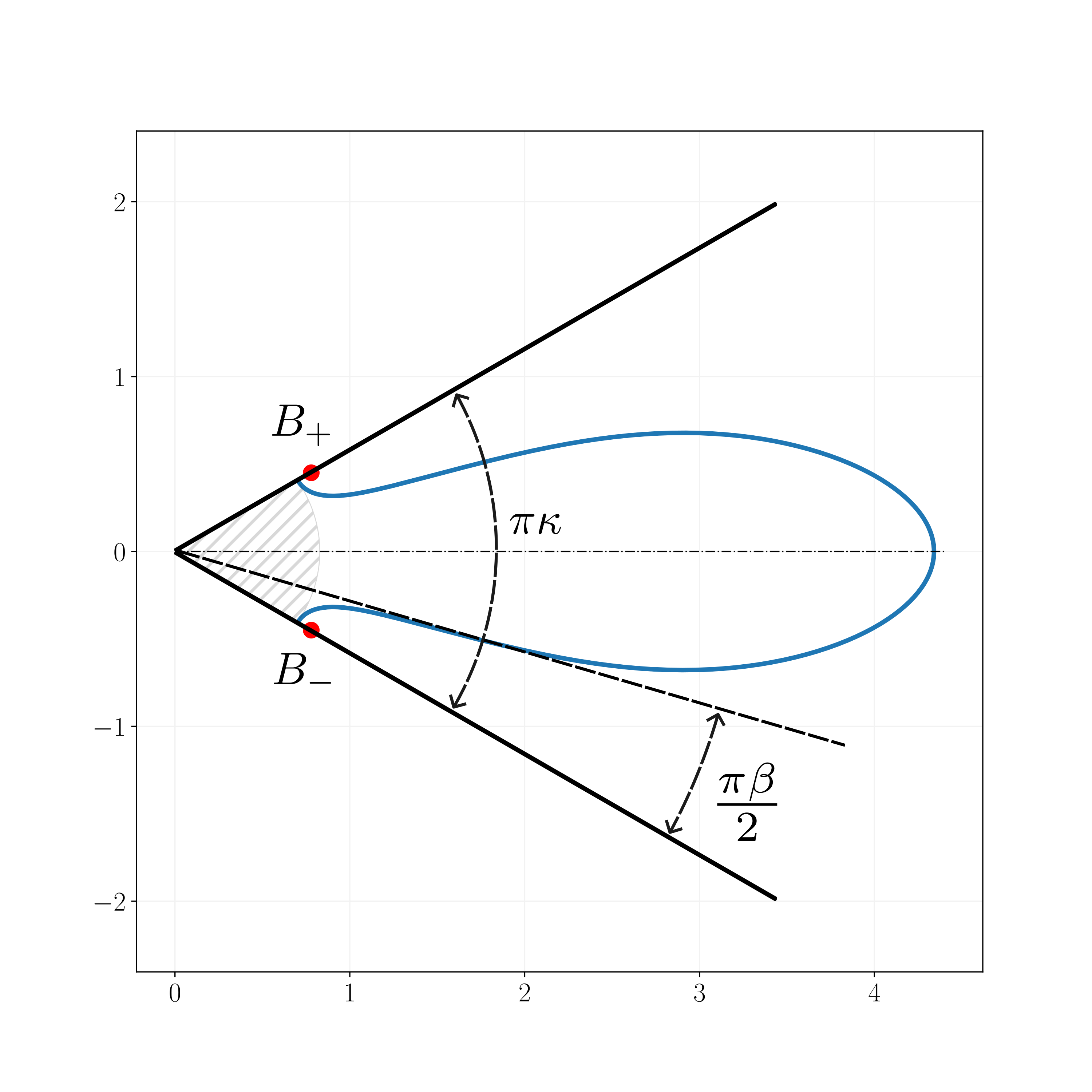
Figure 2: Growing finger in a wedge, described by eq. (15). Constants of motion, $B_{\pm}=B\exp(\pm i\pi\kappa/2)$ are indicated by little red circles at the channel’s walls. We do not indicate here the stagnation points since they almost coincide with $B_{\pm}$. The dashed sector is the unphysical part of the total area.

$$\lambda(\theta)=\frac{\alpha}{\theta}=1-\frac{\beta}{\kappa},$$ (13)

which becomes a function of $\theta$ after selection. The continuum of self-similar solutions in a wedge [2, 61, 62, 63] (a counterpart of the eq. (9) for a channel) reads

$$z(t,w)=r(t)w(1-w^{-2/\kappa})^{\beta}{}_{2}F_{1}{\left(\genfrac{.}{.}{0.0pt}{}{\beta{\mathchar 44\relax}\mskip 8.0mu\beta-\kappa}{1-\kappa};w^{-2/\kappa}\right)}.$$ (14)

Here $z(t,\exp(i\phi))$ is an interface of a growing finger, parametrized by $\phi\in[0,2\pi]$, $r(t)$ is a conformal radius of the conformal mapping, $z(t,w)$, $r(t)=\lim_{w\to\infty}|\partial_{w}z(t,w)|$.

Again, as in a rectangular geometry, we need instead of self-similar solutions (14) to find the family of unsteady non-self-similar solutions for a growing finger in a wedge (a counterpart of (10) for a channel). We found this unsteady asymptotic solution, valid when the unsteady finger evolution’s shape is close to the self-similar one described by (14). We found it by taking the evolution of isobars (level sets in front of the self-similar interface). The solution is:

$$z=r\frac{w}{a}\left(1-\left(\frac{w}{a}\right)^{-2/\kappa}\right)^{\beta}{}_{2}F_{1}{\left(\genfrac{.}{.}{0.0pt}{}{\beta{\mathchar 44\relax}\mskip 8.0mu\beta-\kappa}{1-\kappa};\left(\frac{w}{a}\right)^{-2/\kappa}\right)},$$ (15)

and the criterion of its validity is $1-a\ll 1$. A typical interface described by this solution is schematically shown in blue in Fig. 2.

The finger area $\mathcal{A}$ is readily calculated, by plugging $z(t,w)$ from the last equation into the identity

$$\mathcal{A}=\frac{1}{2\pi i}\oint_{|w|=1}\bar{z}(1/w)dz(w).$$ (16)

Just as in a rectangular geometry (above), there is a constant of motion, $B=z(t,1/a(t))$, which connects $r(t)$ and $a(t)$ in (15):

$$B=ra^{-2}\left(1-a^{4/\kappa}\right)^{\beta}{}_{2}F_{1}{\left(\genfrac{.}{.}{0.0pt}{}{\beta{\mathchar 44\relax}\mskip 8.0mu\beta-\kappa}{1-\kappa};a^{4/\kappa}\right)}$$ (17)

Geometrically $B$ is a distance from the origin, $z=0$, to the intersections of the interface with walls of the wedge (minus a tiny positive correction, not written here to save space). There are two of these intersections, equaled in size because of the symmetry of the growing finger with respect to its central line as shown in Fig. 2.

Analytically $B$ is the branching point of a Riemann surface of a Schwarz function, defined at the interface as $\bar{z}=S(t,z)$ (see details in [64, 30]). Remarkably all singularities of $S(t,z)$ outside the interface are constant in time, so $B$ does not depend on time.

Reduced area. Just as in a channel case, we eliminate the unphysical part of the growing finger, which is the circular sector with a radius $B$ (see Fig. 2), since it depends on the initial conditions. In other words, a pattern completes its formation and acquires the asymptotic shape when the intersection of the interface with the walls reaches the stagnation point. In experiments, this happens after competition between interacting fingers, when a single finger survived. Thus only the finger area without this unphysical part is considered for selection.

Selection. So, we subtract from the full finger area, ${\mathcal{A}}$, the area of this circular sector,

$${\mathcal{A}}_{0}(\beta,\kappa,r(t),a(t))={\mathcal{A}}(\beta,\kappa,r(t),a(t))-\\ -\pi B(\beta,\kappa,r(t),a(t))^{2}\kappa/2,$$ (18)

maximize this $\mathcal{A}_{0}$ with respect to $\beta$ at given $\kappa=\theta/\pi$, $r(t)$, and $a(t)$, and plot resulting $\lambda=\pi(1-\beta)/\theta$ as a function of $\theta$ in Fig. 3.

By comparing our results (orange circles) with results obtained by using the “asymptotic beyond all orders” with inclusion of surface tension (blue triangles) we observe an excellent agreement (the maximal discrepancy is about 1.5%).

The eq. (18) is accurately approximated as

$${\mathcal{A}}_{0}(\beta,\kappa,r,a)=\frac{\pi r^{2}\kappa}{2}\frac{\Gamma(1-\kappa)\Gamma(-\kappa)}{\Gamma(\beta-\kappa)\Gamma(1-\beta-\kappa)}-\\ -\frac{\pi r^{2}(\kappa-\beta)}{2(\kappa/4)^{2\beta}}\frac{\Gamma^{2}(1-\kappa)\Gamma^{2}(1-2\beta)}{\Gamma^{2}(1-\beta-\kappa)\Gamma^{2}(1-\beta)}(1-a)^{2\beta}.$$ (19)

The error between (18) and (19) is practically unnoticeable as one can see in Fig. 3.

In a wedge with the right angle, $\theta=\pi/2$, eq. (19) can be further simplified. In the leading order in $1-a\ll 1$ it reads:

$${\mathcal{A}}_{0}(\beta,1/2,r,a)=\frac{\pi r^{2}(1-2\beta)}{4}\left(\cos\pi\beta-2^{2\beta}(1-a)^{2\beta}\right).$$ (20)

For $a=1-10^{-7}$ (as shown in Fig. 3) this function reaches its maximum when $\beta=0.077$, so that the selected $\lambda=0.85$. It coincides with $\lambda$ in the article [65] about selection by surface tension in $90^{\circ}$ wedge, but differs by .01 from the value $\lambda=0.86$ in [62], which is also selected by surface tension.

Two unexpected observations. When $a(t)$ is not close to 1 the finger has not yet formed its self-similar asymptotic shape, given by (14), so it is too early to test a pattern for selection: one should wait until growing $a(t)$ enters the vicinity of 1, so that $1-a\ll 1$. Then the shape of the finger is finally formed at $a(t)=1-10^{-7}$ (as shown in Fig. 3), and subsequent evolution is not expected to change the selected value of $\beta$ at given $\kappa$. For earlier times the shape has not formed yet, as said above, so it gives lesser than an asymptotic value of $\beta$.

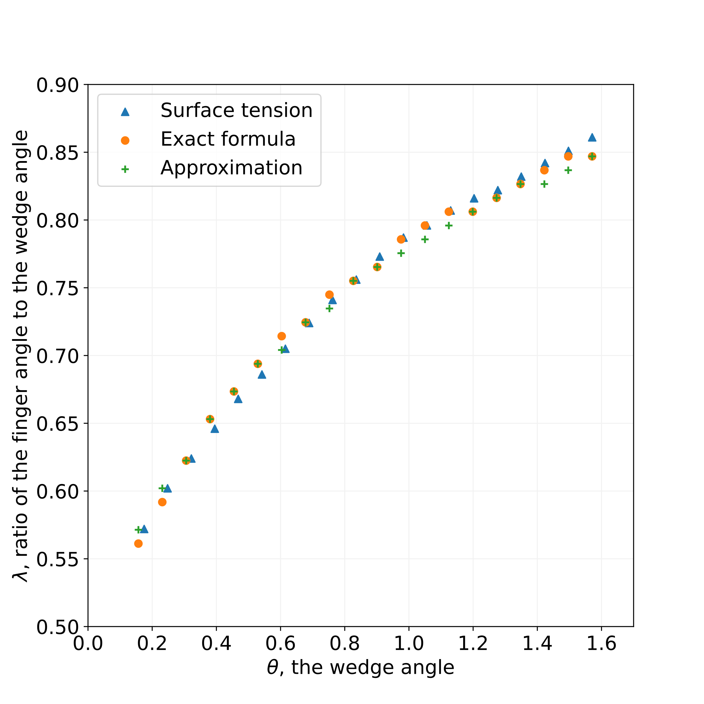
Figure 3: Blue triangles – selection by surface tension (data taken from [62]), orange circles – our selection by exact formula (18), green crosses – selection by approximation (19). The parameter $a(t)$ here equals $a(t)=1-10^{-7}$.

(i) But as we unexpectedly found, for larger values of $a(t)$, that is for larger times, the selected value of $\beta$ gradually loses its accuracy. This is because the area ${\mathcal{A}}$ grows in time contrary to the second term in the RHS of (18), which stays constant in time, so in a long time limit a contribution of the second term in (18), which is crucial for selection, becomes negligible. This explains, we believe, why the accuracy of the selected value worsens for very large $t$, and in the limit $t\to\infty$ the selection disappears entirely.

(ii) It is also very surprising that the critical value of $a(t)$ given above is the same for all wedge angles, $0^{\circ}<\theta\leq 90^{\circ}$.

Future work on selection in a wedge must shed light on both these unexpected observations.

Inevitability of tip-splittings. A local curvature of a self-similarly growing finger decreases as the inverse square root of time. Since surface tension $\sigma$ (neglected here) is always multiplied by curvature, then the effective surface tension, $\sigma(t)$, decreases in time in the same way after rescaling to the time-independent picture with $r(t)=1$. Thus the stability threshold, $\nu_{c}=1.3\exp(-.6\sqrt{(}\mu V/\sigma(t)))$ [66, 67] ($V$ is a local front velocity, and $\mu$ is oil viscosity) decreases in time, so the interface eventually loses stability via tip-splitting. The finger in a channel, on the contrary, stays stable, if to keep noise below the threshold. So the formulae for self-similar patterns written above become invalid after the the first bifurcation (tip-splitting).

No attractor. Motivated by the success of selections in a channel [4, 46, 47, 48] without surface tension, we expected the attractor of (7) to be the selected pattern in a wedge. Since we did not find the attractor (maybe there is no such in a wedge, contrary to a channel), an extra information beyond eq. (7) was needed for selection. This additional information appears to be the entropy (8) in a form of the pattern area, ${\mathcal{A}}_{0}$, in (18) associated with each member of the continuous family (15).

III.4 Universal fjord opening angle

Experimentalists at U. of Texas took a less traditional path of studying viscous fingering in Hele-Shaw cells by shifting attention from fingers to fjords, which separate growing fingers [3]. Wedge geometry is typical and ubiquitous in unstable growth since a growing interface is full of virtual wedges – fragments between centerlines of each pair of adjacent fjords surrounding a growing finger. These centerlines, which are virtual walls as shown in Fig. 4, are streamlines, and so are impenetrable by surrounding fluid. In other words they hermetically separate adjacent virtual wedges (unless the cases when fjords eventually merge).

Fjords are stable and robust, contrary to less predictable fingers because of their unstable evolution. This is a good reason of attracting attention to fjords. Another (and not less remarkable) feature of fjords is that they are the building blocks of exact solutions of the Laplacian growth equation without surface tension (7). More precisely, all fjords geometric characteristics (vertices locations, directions, and shape details) are constants of motion of the eq. (7) represented by the singularities of the Schwarz function [37, 38, 63, 68, 57].

Scientists from Texas posed a new selection riddle by discovering the universal fjords’ opening angle [3] – their experiments in both rectangular and circular Hele-Shaw cells yield fjords opening at a universal angle of $8.0^{\circ}\pm 1.0^{\circ}$. This selection rule holds for a wide range of pumping rates and fjord lengths, widths, and directions.

Previous subsection results must be applicable to these virtual wedges if their centerlines (virtual walls) are straight. The fjord angle (the difference between wedge and finger angles) equals $\pi\beta$ in our terms defined above. If it has a universal value, $\pi\beta_{0}$, which does not depend on the wedge angle for a noticeable range of $\theta$, then the plot in Fig. 3 should fit the formula,

$$\lambda(\theta)=1-\pi\beta_{0}/\theta,$$ (21)

for a constant $\beta_{0}$.

This formula indeed fits our plot in Fig. 3 well for $\pi\beta_{0}=11.7^{\circ}$ for $35^{\circ}<\theta<90^{\circ}$, and coincides with one obtained numerically by using surface tension in [62]. The coincidence is unsurprising, since the result follows from the same plot in Fig. 3, with (almost) no difference between our data (orange circles in Fig. 3) and the data used in [62] (blue triangles). Experiments in a wedge [2] provide a somewhat lower value, that is $10.0^{\circ}$ valid for $20^{\circ}<\theta<90^{\circ}$. The authors of [2] write about the formula, $\lambda(\theta)=1-10^{\circ}/\theta$, they obtained from measurements: “This empirical law is unexplained and could be due to a mere coincidence.”

To summarize, our results confirm the universal fjord angle, $11.7^{\circ}$ for wedges angles $35^{\circ}<\theta<90^{\circ}$, obtained earlier in [62], but cannot explain the discrepancy with somewhat lower experimental values $10.0^{\circ}$ for real [2] and $8.0^{\circ}\pm 1.0^{\circ}$ and for virtual [3] wedges respectively.

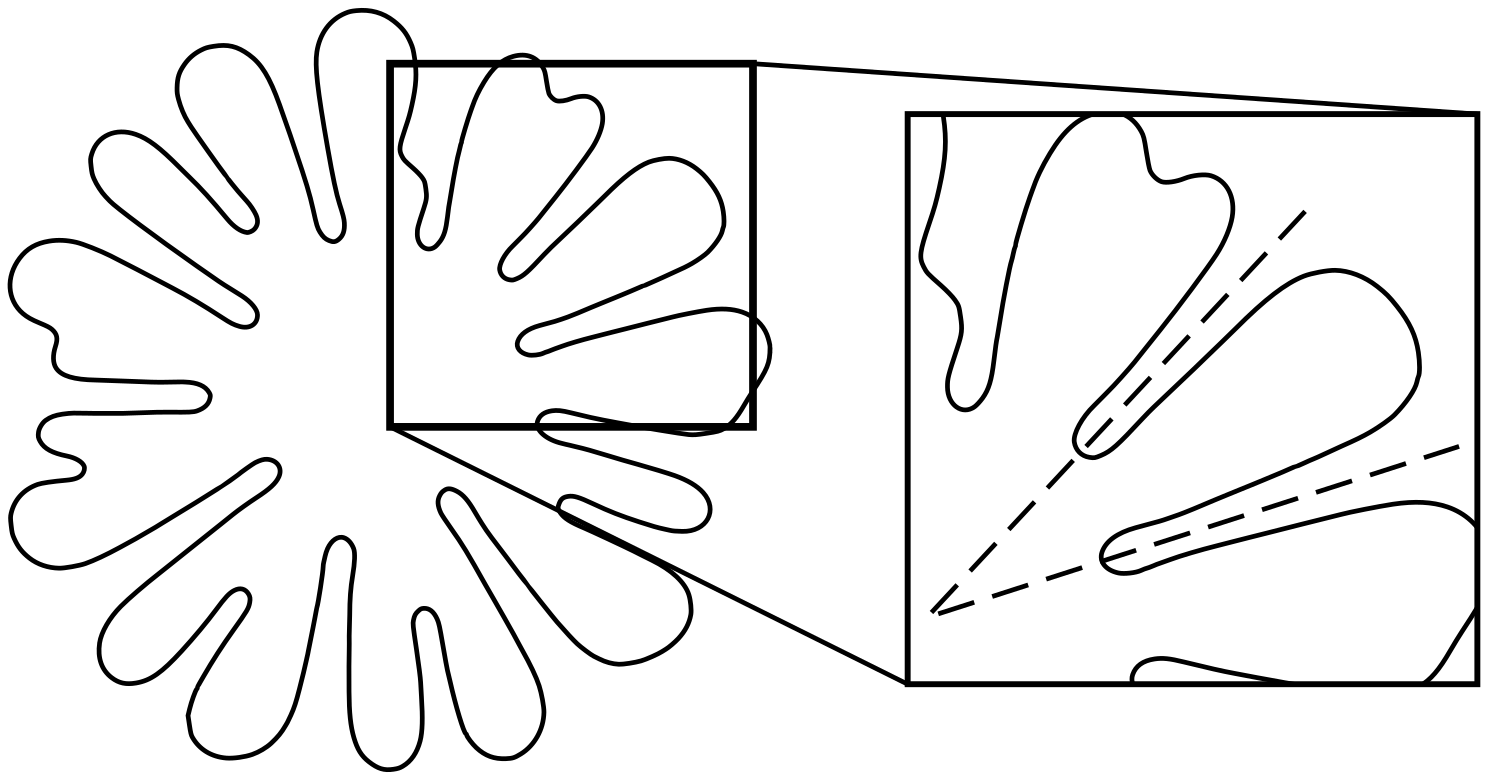
Figure 4: A wedge-like fragment of growing interface in radial geometry (between dashed lines). The centerlines of two fjords surrounding a growing finger form the walls of this virtual wedge.

IV Conclusion

A straightforward variational principle was derived and applied to well-known pattern selection problems in a Hele-Shaw cell in rectangular and wedge geometries. For a finger in a channel this is the second demonstration of selection without surface tension after [4]. The obtained results are in excellent agreement with the experiments.

V Acknowledgment

The authors appreciate discussions with J. E. Pearson and V. Fradkov and their interest to this subject.

VI Funding

The work of O.A. was supported by the Russian Science Foundation grant 19-71-30002

References

- [1] P. G. Saffman and G. I. Taylor, “The penetration of a fluid into a porous medium or Hele-Shaw cell containing a more viscous liquid,” Proc. R. Soc. Lon., vol. 245, no. 1242, pp. 312–329, 1958.
- [2] H. Thomé, M. Rabaud, V. Hakim, and Y. Couder, “The Saffman–Taylor instability: From the linear to the circular geometry,” Phys. Fluids A, vol. 1, pp. 224–240, 02 1989.
- [3] L. Ristroph, M. Thrasher, M. B. Mineev-Weinstein, and H. L. Swinney, “Fjords in viscous fingering: Selection of width and opening angle,” Phys. Rev. E, vol. 74, p. 015201, Jul 2006.
- [4] M. Mineev-Weinstein, “Selection of the Saffman-Taylor finger width in the absence of surface tension: An exact result,” Phys. Rev. Lett., vol. 80, pp. 2113–2116, Mar 1998.
- [5] A. Kolmogorov, I. Petrovskii, and N. Piscounov, “Étude de l’équation de la diffusion avec croissance de la quantité de matiére et son application a un probléme biologique,” Moscou Univ. Math. Bull., vol. 1, pp. 1–25, 01 1937.
- [6] G. I. Taylor, “The instability of liquid surfaces when accelerated in a direction perpendicular to their planes. I,” Proc. R. Soc. Lon., vol. 201, no. 1065, pp. 192–196, 1950.
- [7] L. Landau, “On the theory of slow combustion,” Acta Physicochim. USSR, vol. 19, p. 77, 1944.
- [8] Y. Zeldovich and G. Barenblatt, “Theory of flame propagation,” Combustion and Flame, vol. 3, pp. 61–74, 1959.
- [9] I. M. Gel’fand, “Some problems in the theory of quasilinear equations,” Uspekhi Matem. Nauk, vol. 14, no. 2, pp. 87–158, 1959.
- [10] N. F. Mott, “Brittle fracture in mild steel plates,” Engineering, vol. 165, no. 16, p. 408, 1948.
- [11] G. Barenblatt, “The mathematical theory of equilibrium cracks in brittle fracture,” Adv. Appl. Mech., vol. 7, pp. 55–129, 1962.
- [12] G. P. Ivantsov, “Temperature field around spherical, cylinder and needle-like dendrite growing in supercooled melt,” Dokl. Akad. Nauk SSSR, vol. 58, pp. 567–569, 1947.
- [13] J. S. Langer, “Instabilities and pattern formation in crystal growth,” Rev. Mod. Phys., vol. 52, pp. 1–28, Jan 1980.
- [14] Sir Horace Lamb, Hydrodynamics, vol. 3. New York: Dover publications, 1945.
- [15] L. Onsager, “Reciprocal relations in irreversible processes. I.,” Phys. Rev., vol. 37, pp. 405–426, Feb 1931.
- [16] O. Alekseev and M. Mineev-Weinstein, “Stochastic Laplacian growth,” Phys. Rev. E, vol. 94, p. 060103, Dec 2016.
- [17] O. Alekseev and M. Mineev-Weinstein, “Theory of stochastic Laplacian growth,” J. Stat. Phys., vol. 168, pp. 68–91, Jul 2017.
- [18] L. D. Landau and E. M. Lifshits, Quantum Mechanics: Non-Relativistic Theory, vol. v.3 of Course of Theoretical Physics. Oxford: Butterworth-Heinemann, 1991.
- [19] E. Stückelberg, “Theory of inelastic collisions between atoms,” Helv. Phys. Acta, vol. 5, pp. 369–423, 1932.
- [20] V. Pokrovskii and I. Khalathikov, “On the problem of above-barrier reflection of high-energy particles,” Sov. Phys. JETP, vol. 13, pp. 1207–1210, 1961.
- [21] M. D. Kruskal and H. Segur, “Asymptotics beyond all orders in a model of crystal growth,” Stud. Appl. Math., vol. 85, no. 2, pp. 129–181, 1991.
- [22] B. I. Shraiman, “Velocity selection and the Saffman-Taylor problem,” Phys. Rev. Lett., vol. 56, pp. 2028–2031, May 1986.
- [23] D. C. Hong and J. S. Langer, “Analytic theory of the selection mechanism in the Saffman-Taylor problem,” Phys. Rev. Lett., vol. 56, pp. 2032–2035, May 1986.
- [24] R. Combescot, T. Dombre, V. Hakim, Y. Pomeau, and A. Pumir, “Shape selection of Saffman-Taylor fingers,” Phys. Rev. Lett., vol. 56, pp. 2036–2039, May 1986.
- [25] D. A. Kessler, J. Koplik, and H. Levine, “Pattern selection in fingered growth phenomena,” Adv. Phys, vol. 37, no. 3, pp. 255–339, 1988.
- [26] H. Segur, S. Tanveer, and H. Levine, eds., Asymptotics beyond All Orders, vol. 284 of NATO ASI Series B. New York: Plenum Press, 1991.
- [27] P. G. Saffman, “Viscous fingering in Hele-Shaw cells,” J. Fluid Mech., vol. 173, pp. 73–94, 1986.
- [28] P. G. Saffman, “Selection mechanisms and stability of fingers and bubbles in Hele-Shaw cells,” IMA J. Appl. Math, vol. 46, pp. 137–145, 01 1991.
- [29] A. P. Aldushin and B. J. Matkowsky, “Extremum principles for selection in the Saffman–Taylor finger and Taylor–Saffman bubble problems,” Phys. Fluids, vol. 11, pp. 1287–1296, 06 1999.
- [30] M. Mineev-Weinstein, P. B. Wiegmann, and A. Zabrodin, “Integrable structure of interface dynamics,” Phys. Rev. Lett., vol. 84, pp. 5106–5109, May 2000.
- [31] C. S. Gardner, J. M. Greene, M. D. Kruskal, and R. M. Miura, “Method for solving the korteweg-devries equation,” Phys. Rev. Lett., vol. 19, pp. 1095–1097, Nov 1967.
- [32] B. Shraiman and D. Bensimon, “Singularities in nonlocal interface dynamics,” Phys. Rev. A, vol. 30, pp. 2840–2842, Nov 1984.
- [33] S. D. Howison, J. R. Ockendon, and A. A. Lacey, “Singularity development in moving-boundary problems,” Q. J. Mech. Appl. Math., vol. 38, pp. 343–360, 08 1985.
- [34] M. Mineev, “A finite polynomial solution of the two-dimensional interface dynamics,” Phys. D, vol. 43, no. 2, pp. 288–292, 1990.
- [35] S. D. Howison, “Fingering in Hele-Shaw cells,” J. Fluid Mech., vol. 167, pp. 439–453, 1986.
- [36] D. Bensimon and P. Pelcé, “Tip-splitting solutions to a Stefan problem,” Phys. Rev. A, vol. 33, pp. 4477–4478, Jun 1986.
- [37] M. B. Mineev-Weinstein and S. P. Dawson, “Class of nonsingular exact solutions for Laplacian pattern formation,” Phys. Rev. E, vol. 50, pp. R24–R27, Jul 1994.
- [38] S. P. Dawson and M. Mineev-Weinstein, “Long-time behavior of the N-finger solution of the Laplacian growth equation,” Phys. D, vol. 73, no. 4, pp. 373–387, 1994.
- [39] M. Mineev-Weinstein and O. Kupervasser, “Finger competition and formation of a single Saffman-Taylor finger without surface tension: an exact result,” arXiv:patt-sol/9902007.
- [40] J. Hadamard, “Sur les problèmes aux dérivées partielles et leur signification physique,” Princeton University Bulletin, pp. 49–52, 1902.
- [41] A. N. Tikhonov, “On the stability of inverse problems,” Dokl. Akad. Nauk SSSR, vol. 39, pp. 195–198, 1943. in Russian.
- [42] A. N. Tikhonov, “On the solution of ill-posed problems and the method of regularization,” Dokl. Akad. Nauk SSSR, vol. 151, pp. 501–504, 1963. in Russian.
- [43] A. N. Tikhonov, “On the regularization of ill-posed problems.,” Dokl. Akad. Nauk SSSR, vol. 153, pp. 49–52, 1963. in Russian.
- [44] A. N. Tikhonov and V. Y. Arsenin, Solutions of ill-posed problems. New York: Wiley, 1977.
- [45] M. M. Lavrent’ev, V. G. Romanov, and S. P. Shishatskii, Ill-Posed Problems of Mathematical Physics and Analysis, vol. 64 of Translations of Mathematical Monographs. American Mathematical Society, 1986.
- [46] G. L. Vasconcelos, L. P. Cordeiro, A. A. Brum, and M. Mineev-Weinstein, “Full dynamics of a bubble in a Hele-Shaw channel and velocity selection without surface tension.” (to appear).
- [47] A. H. Khalid, N. R. McDonald, and J.-M. Vanden-Broeck, “On the motion of unsteady translating bubbles in an unbounded Hele-Shaw cell,” Phys. Fluids, vol. 27, p. 012102, 01 2015.
- [48] G. L. Vasconcelos and M. Mineev-Weinstein, “Selection of the Taylor-Saffman bubble does not require surface tension,” Phys. Rev. E, vol. 89, p. 061003, Jun 2014.
- [49] M. Mineev-Weinstein and G. L. Vasconcelos, “Multiple bubble dynamics and velocity selection in Laplacian growth without surface tension,” Phys. D, vol. 459, p. 134032, 2024.
- [50] G. Taylor and P. G. Saffman, “A note on the motion of bubbles in a Hele-Shaw cell and porous medium,” Q. J. Mech. Appl. Math., vol. 12, pp. 265–279, 01 1959.
- [51] S. Tanveer, “New solutions for steady bubbles in a Hele–Shaw cell,” Phys. Fluids, vol. 30, pp. 651–658, 03 1987.
- [52] T. A. Witten and L. M. Sander, “Diffusion-limited aggregation, a kinetic critical phenomenon,” Phys. Rev. Lett., vol. 47, pp. 1400–1403, Nov 1981.
- [53] R. Courant, Dirichlet’s principle, conformal mapping, and minimal surfaces, vol. 3 of Pure and applied mathematics: a series of texts and monographs. New York: Interscience Publishers, 1950.
- [54] M. Lavrentev and B. Shabat, Methods of the theory of function of complex variable. Moscow: Nauka, 1987.
- [55] I. K. Kostov, I. Krichever, M. Mineev-Weinstein, P. B. Wiegmann, and A. Zabrodin, “Tau function for analytic curves,” in Introductory Workshop on Random Matrix Models and their Applications, 5 2000.
- [56] O. Agam, E. Bettelheim, P. Wiegmann, and A. Zabrodin, “Viscous fingering and the shape of an electronic droplet in the quantum Hall regime,” Phys. Rev. Lett., vol. 88, p. 236801, May 2002.
- [57] M. Mineev-Weinstein, M. Putinar, and R. Teodorescu, “Random matrices in 2D, Laplacian growth and operator theory,” J. Phys. A, vol. 41, p. 263001, jun 2008.
- [58] P. G. Saffman, “Exact solutions for the growth of fingers from a flat interface between two fluids in a porous medium or Hele-Shaw cell,” Q. J. Mech. Appl. Math., vol. 12, pp. 146–150, 01 1959.
- [59] G. Herglotz, “Über die analytische fortsetzung des potentials ins innere der anziehenden massen,” Preisschr. der Jablonowski gesselschaft, vol. 44, 1914.
- [60] D. Khavinson, M. Mineev-Weinstein, and M. Putinar, “Planar elliptic growth,” Complex Anal. Oper. Theory, vol. 3, pp. 425–451, 2009.
- [61] M. Ben Amar, “Viscous fingering in a wedge,” Phys. Rev. A, vol. 44, pp. 3673–3685, Sep 1991.
- [62] Y. Tu, “Saffman-Taylor problem in sector geometry: Solution and selection,” Phys. Rev. A, vol. 44, pp. 1203–1210, Jul 1991.
- [63] A. Abanov, M. Mineev-Weinstein, and A. Zabrodin, “Self-similarity in Laplacian growth,” Phys. D, vol. 235, no. 1, pp. 62–71, 2007. Physics and Mathematics of Growing Interfaces.
- [64] P. J. Davis, The Schwarz Function and Its Applications, vol. 17 of The Carus Mathematical Monographs. Buffalo, NY: Mathematical Association of America, 1974.
- [65] E. A. Brener, D. A. Kessler, H. Levine, and W.-J. Rappei, “Selection of the viscous finger in the 90° geometry,” Europhysics Lett., vol. 13, p. 161, sep 1990.
- [66] D. Bensimon, “Stability of viscous fingering,” Phys. Rev. A, vol. 33, pp. 1302–1308, Feb 1986.
- [67] D. Bensimon, L. P. Kadanoff, S. Liang, B. I. Shraiman, and C. Tang, “Viscous flows in two dimensions,” Rev. Mod. Phys., vol. 58, pp. 977–999, Oct 1986.
- [68] A. Abanov, M. Mineev-Weinstein, and A. Zabrodin, “Multi-cut solutions of Laplacian growth,” Phys. D, vol. 238, no. 17, pp. 1787–1796, 2009.