The variable evolution of accretor stars in binary systems due to accretion of increasingly helium-rich material.

Abstract

The recent discovery of examples of intermediate-mass helium stars have offered new insights into interacting binaries. These observations will allow significant improvements in our understanding of helium stars. However, in the creation of these stars their companions may accrete a significant amount of helium-rich stellar material. These creates stars with unusual composition profiles – stars with helium-rich cores, hydrogen-rich lower envelopes and a helium-rich outer envelope. Thus the mean molecular weight reaches a minimum in the the middle of the star rather than continuously decreasing outwards in mass. To demonstrate this structure we present Cambridge STARS model calculations of an example interacting binary systems where the helium-rich material is transferred, and compare it to one where the composition of the accreted mass is fixed to the companion’s surface composition. We show that the helium-rich material leads to the accretor being 0.2 dex hotter and 0.15 dex more luminous than models where the composition is not helium rich. We use a simple BPASS v2.2 population model to estimate that helium-rich mass transfer occurs in 23 per cent of massive binaries that undergo mass transfer. This suggests this is a common process. This binary process has implications for the discrepancy between spectroscopic and gravitational masses of stars, the production of ionizing photons and possibly the modelling of high redshift galaxies.

1 Introduction

The recent discovery of intermediate-mass helium stars in the “gap” between subdwarf helium stars and Wolf-Rayet (WR) stars (Drout et al., 2023; Götberg et al., 2023) is a significant shift in the understanding of the importance of interacting binary stars for stellar populations. These stars are ${\sim}$8{-}25\text{\,}\mathrm{M_{\odot}}$$ progenitors which have their hydrogen envelope stripped via binary interaction. While many groups have investigated the importance of these objects for stellar populations, such as sources of ionizing photons (e.g. Stanway et al., 2016; Götberg et al., 2017; Xiao et al., 2018), hydrogen-poor core-collapse supernovae (e.g. De Donder & Vanbeveren, 1998; Smith et al., 2011; Eldridge et al., 2013; Eldridge & Maund, 2016; Laplace et al., 2021) and gravitational wave transients and/or $\gamma$-ray bursts (e.g. Eldridge et al., 2011; Qin et al., 2018; Stevance et al., 2023; Bavera et al., 2020; Fuller & Lu, 2022), until the direct confirmation of their existence, uncertainty remained over their validity. Importantly, now with the potential detection of these objects, we can begin to test and verify our models of these stars.

The evolution of a star in a binary is complicated in many ways due to the presence of its companion. Notably the two stars may exchange mass, altering the orbit dependent on the mass of the donor and accretor stars. Much study has been devoted to the nature of binary mass transfer (among others, Delgado & Thomas, 1981; Davis et al., 2013; Soberman et al., 1997; Landri et al., 2024). In some studies, such as Dutta & Klencki (2023), which concentrate on the evolution of the mass donor star, the accretor is assumed to be point mass. However, studies where the companion is followed in detail show that the evolution of the accretor can be highly exotic when compared to that for a star from single stellar evolutionary pathways, (e.g. Wellstein et al., 2001; Renzo & Götberg, 2021; Renzo et al., 2023; Menon et al., 2024; Schneider et al., 2024; Wagg et al., 2024).

It is clear from these studies that it is now vital that both the donor star and accretor should be modelled in detail throughout their lifetimes for some binary systems. Furthermore, the accretor stars might as a group provide the most unusual and exotic stellar objects we observe in the Universe, such as chemically homogeneous stars (de Mink et al., 2013; Ghodla et al., 2023) and certain types of chemically peculiar stars (e.g., Hunter et al., 2008; Langer, 2012). Epochs of mass transfer also alter the structure of the constituent stars in a binary (Law-Smith et al., 2020; Klencki et al., 2021; Renzo & Götberg, 2021), in ways emblematic of their past exchanges of material. Although there are implications for the structure and evolution of the accretor (e.g., Packet, 1981; Cantiello et al., 2007; de Mink et al., 2013; Renzo & Götberg, 2021), most works have focused on the structure of the donor as the star which is having its structure most changed (under the assumption that most of the matter is lost to the interstellar medium). However, examining the structure of the accretor requires detailled modelling of both stars throughout their lifetimes, and thus the point-mass approximation becomes insufficient.

Another concern in the evolution of massive binary stars is the discrepancy between the spectroscopic mass and the evolutionary mass (see, for example, Herrero et al., 1992; Massey et al., 2009; Bouret et al., 2013; Massey et al., 2013; McEvoy et al., 2015; Markova et al., 2018; Ramachandran et al., 2018; Bestenlehner et al., 2020). This has commonly been attributed to deficiencies in the physics of model atmospheres (Herrero et al., 1992) or more recently in non-included or not well-understood physics (Bestenlehner et al., 2020). It has been observed through multiple modelling efforts such as BONNSAI (work in Bestenlehner et al. 2020, BONNSAI in Schneider et al. 2014), the work of Maeder (1990) (Herrero et al., 1992), the Geneva tracks (work by Markova et al. 2018, Geneva code by Ekström et al. 2012), and the PoWR code (work by Ramachandran et al. 2018, PoWR code in Gräfener et al. 2002; Hamann & Gräfener 2003; Sander et al. 2015).

Studies of close binaries suggest (Pols, 1994; Vanbeveren et al., 1998; Wellstein et al., 2001; de Mink et al., 2007; Sen et al., 2022) that close binaries experience hydrogen-dominant Case A mass transfer, producing Algol systems where the less massive component fills its Roche lobe (e.g. Leung, 1989). If, however, the mass transfer becomes particularly intense, the hydrogen-rich envelope of the star may become depleted, thus the helium core exposed and the material being accreted may become helium-rich. This material would be provided by nucleosynthesis in the exposed stellar core, further fuelling helium-dominant mass transfer.

Mass transfer which is particularly helium-rich would result in a binary in which thermohaline mixing becomes apparent. This is the process by which heavier atoms sitting atop lighter atoms (as a result of mass transfer) settle towards the core of the star (Ulrich, 1972; Kippenhahn et al., 1980). Thermohaline mixing is dominant when there is a sharp turn-off in the chemical composition profile; if there is a lack of an interface then thermohaline mixing becomes more difficult to predict and model in a 1D stellar modelling code.

In addition, in a close binary any mass transfer (irrespective of chemical composition) would induce unusual tidal effects on the binary due to the changing masses of each constituent star in the gravitational potential of the other. The strength of this interaction is dependent on the radius-separation ratio $R/a$ for each star (Zahn, 1977; Hut, 1981; Hurley et al., 2002), hence tight binaries or systems with extended envelopes would be expected to have strong tidal effects.

Once a star has lost the majority of its hydrogen envelope, its companion has accreted some fraction of it. The efficiency at which the latter occurs is strongly dependent on the mass-transfer rate and the reaction of the secondary star to mass-accretion during the episode of Roche lobe overflow (RLOF). In this work, we investigate the impact of helium-rich material onto an accretor star with an example binary stellar evolution model. We find that while the total mass transfer efficiency is moderate. The efficiency of helium-rich material is high. We also model the subsequent evolution of the accretor star and evaluating how this causes the evolution to differ for a single star with the same mass. We find the future evolution of these stars could explain some unexplained questions in the study of massive star evolution (such as the discrepancy between spectroscopic and evolutionary masses) and possibly recent results on the diversity of mixing profiles from asteroseismology.

The structure of this paper is as follows. First, in section 2, we outline the numerical method used to perform this work. In section 3, we present detailed binary evolution models where both stars have been evolved in detail, to demonstrate the impact on the accreting star of the transfer of helium-rich material from a late-main sequence donor. In section 4, we demonstrate the impact of mass transfer onto companions and show an example of the impact on the accretor’s eventual evolutionary path on the Hertzsprung-Russell (HR) diagram where such stars are more luminous and hotter than single-stars with the same total mass. In section 5 and section 6, we discuss what other phenomena could be linked to this, such as the occurrence of an excess of yellow supergiants (YSGs; Beasor et al., 2023; Dorn-Wallenstein et al., 2023), luminous-blue variables (LBVs; Smith & Tombleson, 2015), Be stars and possibly explain the diversity of mixing profiles found by asteroseismology. In section 7, we review and conclude.

2 Numerical method

To model the detailed response of the binary, we use a modified version of the Cambridge STARS code, which was first described in Eggleton (1971) and was last comprehensively described in Stancliffe & Eldridge (2009). It simultaneously solves the equations of structure and evolution of both stars, and the orbital parameters. This code is being improved upon to in the future potentially include in the Binary Population and Spectral Synthesis (BPASS; Eldridge et al., 2017) code suite. We note that the last common version of the Cambridge STARS code between the BPASS v2.2 models and those from this code was described in Eldridge & Tout (2004a) and Eldridge & Tout (2004b).

We have made refinements to the code surrounding mass transfer and the treatment of Roche lobe overflow. In particular, we have introduced a new time-step control mechanism (building atop the one described in Stancliffe & Eldridge, 2009), whereby as the star begins to exceed its Roche lobe, we slowly decrease the timestep as a function of the amount of the star by radius that exists outside of its Roche lobe. Since the time-step control described in Stancliffe & Eldridge (2009) is based on the modulus of the total change of all parameters (excluding luminosity), rapid changes in the model such as through RLOF would cause the code to fail.

We assume that the initial composition of the primary star is (by mass fraction) 70 per cent hydrogen, 28 per cent helium, and the remaining 2 per cent in metals. We assume a standard solar metallicity of $Z_{\odot}=0.020$, with an equivalent abundance mix of elements as described in section 2.1.1 of Eldridge et al. (2017), which is in turn based on Grevesse & Noels (1993). The code only computes the changes in the abundance of hydrogen, helium-4, helium-3, carbon, nitrogen, oxygen and neon. Other elements are assumed to not vary. As pointed out by Stancliffe et al. (2005), other elements and isotopes are not sufficiently energetic to alter the structure or evolution of the star, and are thus not included in this model. Mixing is performed using the Schwarzchild criterion, using a convective overshooting parameter $\delta_{\text{ov}}$ of 0.12, and no thermohaline mixing to understand the biggest impact that helium-rich mass transfer could have.

2.1 Mass loss rates

Our main mass transfer surface boundary condition is

$$\dot{M}=\dot{M}_{\text{wind}}-\dot{M}_{\text{Bondi}}+\dot{M}_{\text{RLOF}}-\dot{M}_{\text{acc}}.$$ (1)

This employs modified versions of the mass-loss routines given in Eldridge et al. (2017) for the mass loss due to stellar winds, as well as accretion from a companion’s stellar wind as described in Bondi & Hoyle (1944); Hurley et al. (2002). We detail the modifications we have made below.

2.1.1 Wind mass loss

Accounting for mass-loss by stellar winds (i.e., computing the $\dot{M}_{\text{wind}}$ term in Equation 1) involves the use of a number of mass-loss rates prescriptions for the various stellar types the model might experience. In this work we use the same scheme as outlined by Eldridge et al. (2017). We use as our base mass-loss rates those of de Jager et al. (1988) for all stars unless the stars are O stars ($27.5\leq T_{\text{eff}}~{}/~{}\unit{\kilo}\leq 50$), in which case we switch to those from Vink et al. (2001). We interpolate around the bistability jump between B-type and O-type stars using the method in Vink et al. (2001). When the hydrogen envelope becomes depleted and the surface hydrogen mass fraction drops below 0.4 and the surface temperature is above $1\text{\times}{10}^{4}\text{\,}\mathrm{K}$ we switch on the rates of Nugis & Lamers (2000), using their WN mass-loss rates until the carbon and oxygen dominate the surface composition when we switch to the WC mass-loss rates. We note that we smooth the transition between these different mass-loss rates in surface temperature or surface hydrogen abundance to help numerical stability and avoid sharp changes in the stellar wind mass-loss rate.

2.1.2 Bondi-Hoyle wind accretion

The mean accretion rate (in the absence of RLOF) onto the companion is that given in Bondi & Hoyle (1944), namely

$$\dot{M}_{\text{Bondi}}=\min\left[-\left(\frac{GM_{2}}{v_{\text{W}}^{2}}\right)^{2}\frac{\alpha_{\text{W}}}{2a^{2}}\frac{1}{\left(1+v^{2}\right)^{3/2}},~{}0.8\right]\dot{M}_{\text{companion wind}},$$ (2)

where we have assumed a circular orbit (as close binaries have approximately circular orbits), that the orbital velocity is given by

$$v^{2}=\frac{G\left(M_{1}+M_{2}\right)}{av_{\text{W}}^{2}},$$ (3)

and that the wind speed is given by

$$v_{\text{W}}=2\beta_{\text{W}}\frac{GM_{1}}{R_{1}},$$ (4)

where, in both equations, $M_{1},M_{2},a$, and $R_{1}$ are the primary mass, secondary mass, orbital separation, and primary radius respectively. The two free accretion parameters are taken to be $\alpha_{\text{W}}=\frac{3}{2}$ (Boffin & Jorissen, 1988), $\beta_{\text{W}}=7$ (Lamers et al., 1995) for O-type stars.

2.1.3 Roche lobe overflow

The mass loss rate for matter lost through RLOF is given by

$$\dot{M}_{\text{RLOF}}=\min\left[kM^{2}\times\mathcal{R}\left(\frac{R}{R_{\text{RL}}}\right)^{3},0.01\right]$$ (5)

where $\mathcal{R}(x)=\max\left(x,0\right)$, $R_{\text{RL}}$ is the Roche lobe equivalent radius from Eggleton (1983). Here, $k$ is a parameter to control the efficiency of RLOF. We select $k=10^{3}$ which was chosen to ensure stable mass transfer by Stancliffe & Eldridge (2009) based on work by Hurley et al. (2002). We note that $kM^{2}$ is our equivalent to the $F(M_{1})$ parameter in Hurley et al. (2002); Eldridge et al. (2017), though without the maximum mass threshold of $5\text{\,}\mathrm{M_{\odot}}$.

2.1.4 Accretion

We take our accretion rates from Hurley et al. (2002), limiting the accretion rate by the Kelvin-Helmholtz time-scale $T_{\text{KH}}$ of the star and by the critical rotation velocity of the star, that is,

$$\dot{M}_{\text{acc}}=\min\left(\dot{M}_{\text{RLOF}},\frac{M}{T_{\text{KH}}}\mathcal{R}\left(1-\frac{\omega}{0.8\omega_{\text{crit}}}\right)\right),$$ (6)

where $\omega$ is the spin rate of the star assuming non-solid body rotation (i.e., that the star is composed of individually rotating shells of variable thickness governed by the mesh spacing function in Eggleton (1971)). That is to say, the moment of inertia $I$ for a star with $N$ meshpoints is given by

$$I=\frac{2}{5}M_{\text{c}}R_{\text{c}}^{2}+\sum_{k=1}^{N}\frac{2}{3}\left(m_{k}-m_{k+1}\right)r_{k}^{2},$$ (7)

where $m_{k}$ ($r_{k}$) is the mass (radius) internal to meshpoint $k$, and subscript c refers to the central meshpoint, which is assumed to contain a solid sphere. The total spin rate $\omega$ is given by $\omega=\nicefrac{{H_{\text{spin}}}}{{I}}$ for total spin angular momentum $H_{\text{spin}}$.

2.2 Tidal forces

We employ the tidal friction prescription as outlined in sections 2.3.1 and 2.3.2 of Hurley et al. (2002), which is in turn based on Zahn (1977) and Hut (1981), however this mechanism is only turned on once the star has reached a minimum age of $1\text{\,}\mathrm{kyr}$. We write

$$\left.\frac{\mathrm{d}\omega_{\text{orb}}}{\mathrm{d}t}\right|_{i}=-3\left(\frac{k}{\tau}\right)_{\text{c}}q\left(1+q\right)\left(\frac{R_{i}}{a}\right)^{8}H_{\text{orb}}\left(1-\frac{\omega_{\text{spin},i}}{\omega_{\text{orb},i}}\right),$$ (8)

and

$$\left.\frac{\mathrm{d}\omega_{\text{spin}}}{\mathrm{d}t}\right|_{i}=3\left(\frac{k}{\tau}\right)_{\text{c}}\frac{q^{2}}{r_{g}^{2}}\left(\frac{R_{i}}{a}\right)^{6}\omega_{\text{orb},i}\left(1-\frac{\omega_{\text{spin},i}}{\omega_{\text{orb}}}\right),$$ (9)

where $\left(\frac{k}{\tau}\right)_{\text{c}}$ is given by equation 30 of Hurley et al. (2002) (we have used $\tau$ in place of their $T$ for the tidal evolution timescale, to distinguish it from the temperature $T$ elsewhere in this paper), $r_{g}$ is the radius of gyration of the star, and $H_{\text{orb}}$ is the orbital angular momentum. We note that, as with the rest of this work, we have assumed circular orbits.

2.3 Accretion of chemically variable matter

During accretion, the infalling material may have a different composition than the accretor’s surface layer. We allow for variable composition accretion in the following way. If one star is filling its Roche lobe, we set the abundance of the accreted material to the surface abundance of this star. If both stars are filling their Roche lobes, we set the abundance of accreted material to the average of the two surface abundances of both stars.

There are two key reasons why we adopt this particular approach. Firstly, if both stars are filling their Roche lobes, not averaging their abundances would mean that we would be overriding the accretor’s abundance with the donor’s, effectively artificially introducing material into the system.

Secondly, when the two stars are in the contact phase, near-surface mixing would cause the composite accreted material to be mixed in with the star. That is to say, a parcel of material being deposited on to the accretor may displace material from the surface of the accretor into the accretion stream, resulting in a stream that is not “pure” material from the donor. In the instances when we compare to a non-variable composition accretion model, we set the abundance of the accreted material to the abundance of a layer of material next-to-surface on the star. When variable composition accretion is enabled in our figures, we refer to it as “variable accretion”, and “no variable accretion” if it is disabled.

2.4 Simulated model parameters

We consider a binary system with $M_{1,\text{ZAMS}}=$30\text{\,}\mathrm{M_{\odot}}$,M_{2,\text{ZAMS}}=$10\text{\,}\mathrm{M_{\odot}}$,$ and $\log~{}P_{\text{ZAMS}}=$0.6\text{\,}\mathrm{d}$$, one of the binaries in the sample of Richards & Eldridge (in prep.), and one of the potential progenitors of LSS 3074, which is a system most likely in a contact phase with both stars filling their Roche lobes. The initial time-step is taken to be 10 per cent of the Kelvin-Helmholtz time-scale of the primary star. The stars are both assumed to be initially non-rotating, homogeneous with the initial abundances, and the code runs until core helium exhaustion in the donor.

Although this model was initially computed to find binary models that would match LSS 3074 at the present day, we caution that the interpretation of this work is not an investigation into the origins of LSS 3074 as a binary. We consider three scenarios of evolution:

1. In our fiducial model, we enable the modifications made to the chemical composition in subsection 2.3.

2. In our non-variable composition accretion model, we disable the modifications and set the abundance of the accreted material to the next-to-surface abundances of the star.

3. When core helium burning concludes in the donor, we take the output of both accretor models, readjust the timestep to 10 per cent of the thermal timescale of the star, and evolve them as single stars.

This approach to single-star evolution allows us to “stitch” together two sets of models into one continuous path on, say, a HR diagram with minimal discontinuity.

3 The response of a binary companion to the accretion of helium rich material

3.1 The contact phase

When the primary star exceeds its Roche lobe during its main sequence, it begins to efficiently transfer material onto the secondary. This mass transfer shrinks the orbital separation of the binary by about 20 per cent, and causes the secondary to swell and fill its own Roche lobe, forming a contact binary. The evolution around the contact phase is shown in Figure 1, and over the entire evolution in Figure 7. Notably, when the system becomes a contact binary, the separation shrinks dramatically owing to conservation of angular momentum. This results in a final period of $\sim$2.6\text{\,}\mathrm{d}$$.

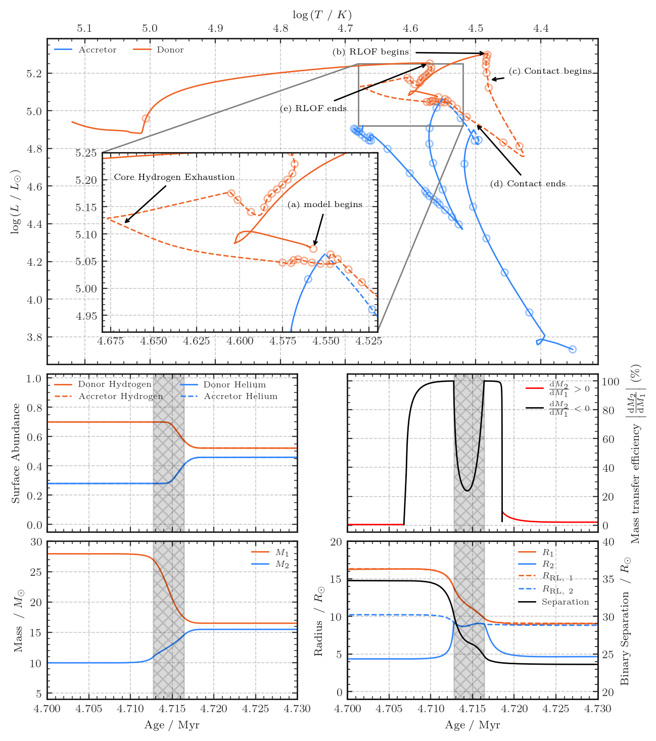
Figure 1: The evolutionary history of a $30+10\text{\,}\mathrm{M_{\odot}}$ binary with an initial period of $\log~{}P=$0.6\text{\,}\mathrm{d}$$. Clockwise from top are the HR diagram, the mass transfer efficiency, the radius/separation, the masses, and the surface abundances. On the HR diagram, the circles represent every 1,000 models, and the dashed lines signify periods when the respective star is undergoing RLOF. Key phases of the evolution of the binary are shown marked on the plot, and the marked stages have the same meanings as in Figure 4 and Table 2. All plots except from the HR diagram show only the region surrounding the contact phase (shown in the black band, lasting approximately $3.7\text{\,}\mathrm{kyr}$) as this is the region of interest. The binary separation is shown in the black line on the right axis of its corresponding plot.

As a potential formation channel of LSS 3074 (Richards & Eldridge in prep.), this contact binary phase is not unexpected. However, the intensity of the mass transfer in the immediate lead-up to this phase does cause helium-rich material to be exposed from the core of the donor star, which is then accreted by its companion. This causes a change in the radii of both stars.

On the one hand, because the donor star is being stripped and has thus lost material, its radius shrinks to as it attempts to re-establish equilibrium. On the other hand, as shown in Table 2, the accretor remains at a roughly constant radius throughout this contact phase, decreasing by only $\sim$0.3\text{\,}\mathrm{R_{\odot}}$$ or 2.7 per cent. There are two reasons for the constancy of the radius:

1. Firstly, throughout the contact phase, the masses begin to equalise as the binary becomes tighter, with a final mass ratio of $q\approx 0.93$ (compared to $q\approx 0.41$ prior to the contact phase). This rising mass ratio and shrinking of the orbit effectively balance each other out, such that the accretor’s Roche lobe follows an approximately constant contour along $R_{\text{RL}}(q,a)$ according to Eggleton (1983).

2. Secondly, the RLOF prescription in Equation 5 reasonably aggressively forces a star to remain within its Roche lobe, via the factor of $k=10^{3}$ in the equation. It is possible for this prescription to generate binaries that substantially overfill $\mathcal{L}_{1}$, and even to fill $\mathcal{L}_{2}$, however this generally requires tighter binaries than considered here.

The process of generating and sustaining the contact phase can be broken down into the following stages, summarised in Figure 2:

1. In the immediate lead-up to the contact phase, the accretor begins to accrete material, causing it to spin up. The rotation rate also increases due to transfer of angular momentum and the accretor approaches 15 per cent of its critical rotation rate.

2. This accretion breaks thermal equilibrium and causes the accretor to expand (Lau et al., 2024, and references therein)

3. The donor decreases in luminosity slightly as the accretor increases in luminosity by an order of magnitude.

4. It then begins to increase in luminosity, but returns the radius to approximately the size it was prior to the onset of RLOF, which is below the expected radius for a star of that luminosity.

5. The abrogation of thermal equilibrium in the accretor powers the contact phase, which lasts for approximately $3.7\text{\,}\mathrm{kyr}$.

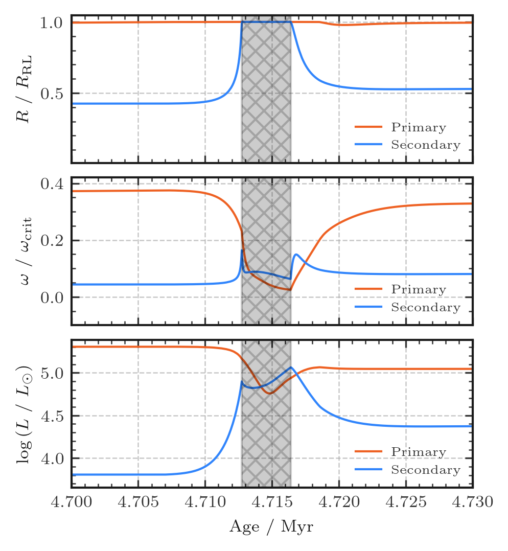
Figure 2: The evolution of the radius as a fraction of Roche lobe radius, rotation rate as a fraction of critical rotation rate, and luminosity of both stars. The black bar on each subplot denotes the contact phase, which lasts $\sim$3.7\text{\,}\mathrm{kyr}$$.

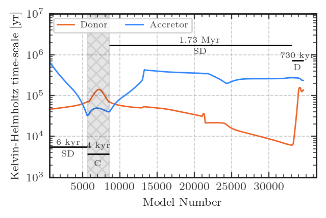
(a) Variable accretion

(b) Non-variable accretion

Figure 3: The Kelvin-Helmholtz time-scales of both stars in the variable and non-variable accretion regime. Here, SD means semidetached (one star filling its Roche lobe), C means contact (both stars filling their Roche lobes), and and D means fully detached (neither star filling its Roche lobe). Not shown is the fully detached phase at the beginning of evolution, which lasts for $4.71\text{\,}\mathrm{Myr}$ and is identical for both cases. Variable accretion prolongs the final detached phase and shrinks the contact phase. The solid black lines show the length $T$o f each phase – thermal equilibrium is broken if $T_{\text{KH}}>T$, i.e., in the first semidetached phase and the contact phase.

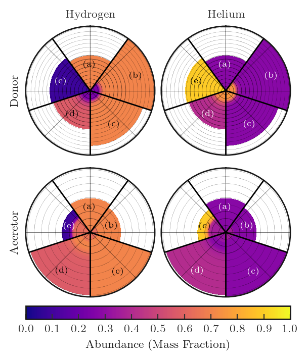
(a) Variable accretion

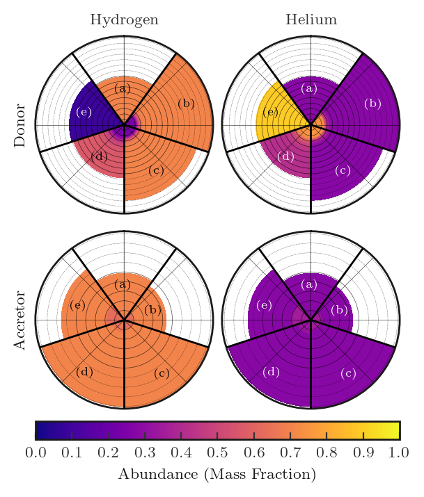
(b) Non-variable accretion

Figure 4: The chemical composition of each star as a function of the stellar radius for the donor and accretor at the five key stages of the binary’s lifetime as detailed in Table 2. Letters are as given in the same table and again in Figure 1. Each grid marking in the radial direction represents $1\text{\,}\mathrm{R_{\odot}}$.

Eventually the accretor shrinks to within its Roche lobe and terminates the contact phase. The reason for this is that the accretor’s mass has increased to such a point that its thermal timescale is now equivalent to the mass transfer rate from the donor star as shown in Figure 3. The accretor is thus able to achieve thermodynamic equilibrium and return to its more compact state. This shrinking is not due to the denser helium-rich material that has been accreted, although we discuss the impact of this below.

3.2 The post-contact phase

At the termination of the contact phase, enough helium-rich material has been accreted that the chemical profile of the star has measurably changed. As is shown in 4(a), in the case of variable composition accretion, the accretor can be broken up into three key layers. The first is the helium-enriched convective core. Sitting atop this core is a layer of hydrogen-rich material, which was the original photosphere of the accretor prior to the onset of mass transfer. Finally sitting on the very top of the accretor is a layer of helium-rich accreted material. The development of this layer leads to the star changing trajectory on the HR diagram compared to if the material had been assumed to be non-variable; this is shown in the inset of Figure 5. The net effect of this helium-rich layer is to produce a star which is hotter and at times more luminous than if the material was non-variable once the accretor shrinks within its Roche lobe. These three layers do not exist in the absence of variable accretion (4(b)), where the turnoff from helium core to mixed envelope is sharper.

Eventually the donor loses enough material that its envelope collapses and it becomes a more compact helium star, shown in 4(a) (from stage D to E). During the (non-RLOF) mass transfer period, we have always assumed that the accretor star accreted all of the transferred material. However, once the accretor fills its Roche lobe, its mass increase becomes limited so an equilibrium is reached, and once the accretor shrinks within its Roche lobe, then the mass transfer rate again increases. We find this leads to an average mass transfer efficiency of 45.02 per cent of material being transferred (the donor star loses $24.10\text{\,}\mathrm{M_{\odot}}$ while the accretor gains $10.85\text{\,}\mathrm{M_{\odot}}$). We can see this inefficiency of the mass transfer in the grey shaded region in the mass panel of Figure 1 – prior to the contact phase, $M_{1}+M_{2}\approx$37\text{\,}\mathrm{M_{\odot}}$$, and after the contact phase $M_{1}+M_{2}\approx$32\text{\,}\mathrm{M_{\odot}}$$. The instantaneous mass transfer efficiency fluctuates during the contact phase, though sits between 30 and 40 per cent throughout, and the accretor continues to gain mass throughout this phase. The ratio of mass transfer rates $\frac{\mathrm{d}M_{1}}{\mathrm{d}t}\div\frac{\mathrm{d}M_{2}}{\mathrm{d}t}=\frac{\mathrm{d}M_{1}}{\mathrm{d}M_{2}}$ in Figure 1 shows that for $\sim$6\text{\,}\mathrm{kyr}$$ prior to, during, and $\sim$3\text{\,}\mathrm{kyr}$$ after the contact phase, mass is indeed transferring between stars (black curve), however outside of this band there are regions where mass is, on the whole, lost to the interstellar medium (red curve). If $\frac{\mathrm{d}M_{1}}{\mathrm{d}M_{2}}$ is positive then typically both stars are losing mass in stellar winds, however if the value is negative then mass transfer is occuring from one star to the other.

Here the efficiency of the mass transfer is determined by the reaction of the accretor and orbit to the mass gain. Together these factors determine how long the star fills its Roche lobe for before the masses of the star become similar to allow the accretor to relax with in the Roche lobe. Attempting to parameterize the mass transfer efficiency for other rapid binary evolution models will require a much more extensive grid than presented here. The closest prescription would appear to be using thermal timescale limited accretion onto the accretor, but this may underestimate the initial amount of mass transferred to the accretor. Only with a more extensive grid of models would this be possible to test.

3.3 Post-mass transfer

Once mass transfer is complete, the evolution of the accretor is highly uncertain. Although the primary has a smooth composition gradient, the secondary’s is quite inhomogeneous, especially immediately on top of the convective core. As shown in 4(a) (segment D, and also in 8(b)), the accretor has a helium-rich core ($Y_{\text{core}}\sim 0.4$) from the result of core hydrogen burning, a hydrogen-rich lower-envelope region sitting atop it, with an upper envelope structure of increasing helium-richness towards surface. It is reasonable to assume such accretor structures must be common among the companions of observed helium dwarfs (see section 5), which makes such stars interesting objects to study in further detail.

The future evolution of these composition gradients will be determined by several factors as discussed by Renzo & Götberg (2021). Firstly, thermohaline mixing may allow the helium rich material to mix into the stellar interior, although the time-scale of this process is not certain – especially considering there is not a sharp composition boundary, but a more gradual gradient. Additionally, if the star is rapidly rotating, rotation-induced mixing (which is not included in these models) may be able to induce further transport of material to smooth out the composition gradient (e.g. Eggenberger et al., 2010). It is pertinent to note here that there is a balancing act between the companion spinning up as it shrinks and the accretion of angular momentum by the primary star into the orbit via tidal synchronisation. As pointed out by Renzo & Götberg (2021), this would create a large level of complexity in the structure and evolution of the secondary, though the composition gradient would act to stabilise the mass transfer though thermohaline mixing (smoothing the gradient, and thus causing the accreted material to similarly have a less variable chemical composition). This suggests that the evolution and mixing profiles will be highly non-linear, and potentially chaotic. We suggest that given the likely large range of mass transfer histories in a full population of stars it is likely that some of the different mixing seen in asteroseismological observations by Pedersen et al. (2021) may be the result of binary mass transfer.

4 Future evolution of the accretor

The altered chemical profile of the secondary star impacts its future evolution. To test this, we evolve the binary using variable and non-variable composition accretion and show the evolution of the secondary in an HR diagram in the bottom panel of Figure 5. When the model terminates (which is after RLOF completes and a CO core begins to develop in the donor, as shown in 8(a) and 8(b)), we take the last converged accretor model and use that as input to a single-star routine. We note that we disable WR mass-loss rates for this process. While the surface temperature and hydrogen abundance of the model is within that expected for WR stars, it is still a hydrogen-burning object, so we calculate the mass-loss rates using the O star mass-loss scheme described in subsection 2.1.

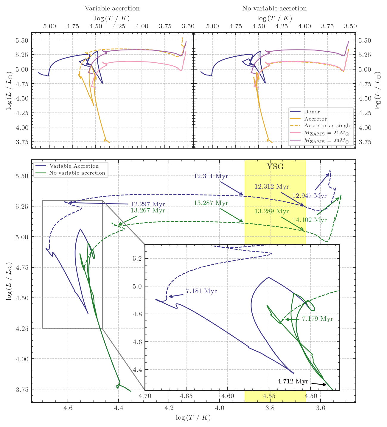
Figure 5: An HR diagram showing the evolution of our model both with (top left) and without (top right) the variable accretion model. The bottom panel shows only the evolution of the secondary. Variable composition accretion produces hotter secondaries than on an equivalent binary with non-variable accretion. The point of divergence between the two models is shortly into the contact phase. The two dashed lines on the bottom HR diagram represent models evolved as the final model of the binary secondary, as a single star, and the yellow band shows the YSG region. Core and surface abundances of the single star models are given in Table 1. On the top HR diagrams, the pink and brown models are single stars evolved with ZAMS masses of 21 and 26 respectively.

		Variable	Standard
	$M~{}/~{}M_{\odot}$	11.31	17.19
	$M_{\text{He}}~{}/~{}M_{\odot}$	10.37	7.52
	$M_{\text{CO}}~{}/~{}M_{\odot}$	7.00	4.82
	$T~{}/~{}K$	3646.53	3305.90
	$\log\left(L~{}/~{}L_{\odot}\right)$	5.50	5.32
	Age / Myr	12.95	14.11
	$R~{}/~{}R_{\odot}$	1417.03	1388.45
Surface	$X_{\text{H}}$	0.40	0.60
	$X_{\text{He}}$	0.58	0.38
	$X_{\text{C}}$	0.00	0.00
	$X_{\text{N}}$	0.01	0.00
	$X_{\text{O}}$	0.00	0.01
	$X_{\text{Ne}}$	0.00	0.00
Core	$X_{\text{H}}$	0.00	0.00
	$X_{\text{He}}$	0.00	0.00
	$X_{\text{C}}$	0.01	0.00
	$X_{\text{N}}$	0.00	0.00
	$X_{\text{O}}$	0.44	0.40
	$X_{\text{Ne}}$	0.55	0.60

Table 1: The profiles of the single star evolutionary tracks in Figure 5 (dashed lines in that figure) as at their ends of evolution. Both models develop similar CO cores, though the variable accretion model does not live as long and becomes less massive than the non-variable accretion.

4.1 Impact on effective surface temperature and luminosity

When we study the evolution of these post-accretion models we see several features. First, the non-variable accretion case behaves similarly to a $21\text{\,}\mathrm{M_{\odot}}$ single star with the same composition evolved from ZAMS. This is because the accretor has a close initial mass of $20.7314\text{\,}\mathrm{M_{\odot}}$. Second, there are no such single-star models which provide a clear match to the accretor case with variable composition accretion. We see the during the main sequence the accretor is approximately $0.2\text{\,}\mathrm{dex}$ hotter in surface temperature, although the luminosity of the star is similar to that of a $26\text{\,}\mathrm{M_{\odot}}$ star. The tracks do become more similar during the Hertzsprung gap and red supergiant branch, though towards the top of the evolution as a red supergiant the accretor model does jump to a slightly hotter surface temperature of about $0.05\text{\,}\mathrm{dex}$.

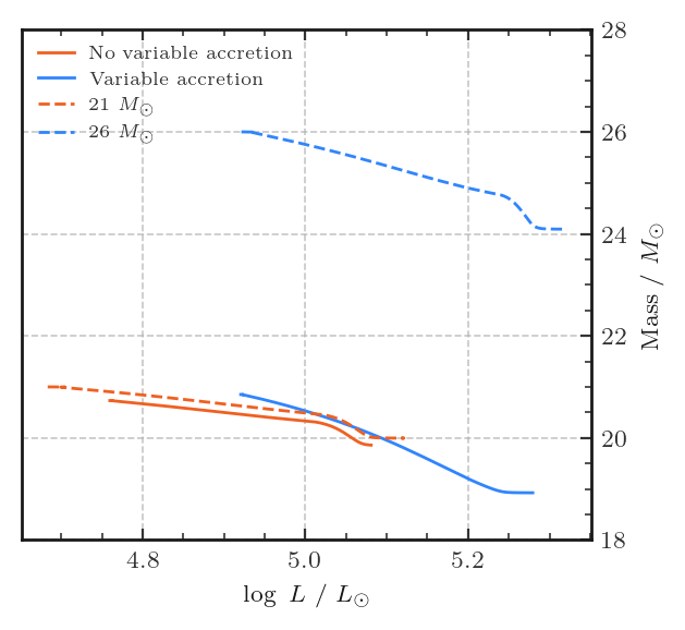
Figure 6: The mass vs. luminosity track in the presence and absence of variable accretion. Also shown are the single-star $21\text{\,}\mathrm{M_{\odot}}$ and $26\text{\,}\mathrm{M_{\odot}}$ models from Figure 5. The region shown in this plot is from ZAMS until core hydrogen exhaustion for each model.

The implications of this are significant. The variable composition accretion model has the luminosity equivalent to a star $5\text{\,}\mathrm{M_{\odot}}$ more massive. This is approximately $0.2\text{\,}\mathrm{dex}$ more luminous than is expected for a single star with the same mass. This and the higher surface temperatures suggest that the contribution of accretor stars to the luminous and ionizing output from stellar populations may have been underestimated in current BPASS spectral synthesis calculations since this effect is not included. This would be an extra boost beyond what is already included in BPASS and could help agreement with modelling high redshift galaxies (e.g., Eldridge & Stanway, 2012, 2022) and the process of reionization (e.g., Stanway et al., 2016; Ghodla et al., 2023)

This also may explain the mass discrepancy for some stars between their spectroscopic and evolutionary masses (e.g. Herrero et al., 1992; Massey et al., 2009; Bouret et al., 2013; Massey et al., 2013; McEvoy et al., 2015; Markova et al., 2018; Ramachandran et al., 2018; Bestenlehner et al., 2020). Comparing the luminosities of our accretors models to single stars models in Figure 6 we can see that that a star with helium-rich accretion has a luminosity similar to a star that is 20 per cent more massive. Such a difference may explain why for some stars’ mass estimates can differ significantly. One implication of this is that compact remnant masses estimated from their stellar companion mass may be overestimated, if the evolution of the companion star has been affected by helium-rich mass transfer.

The surface temperature of the accretor has important implications for the observations of SN progenitors. The donor is massive enough to explode as a type Ib/c SN. A number of observations exist of the pre-SN site of many type Ib/c SNe (e.g. Eldridge et al., 2013; Eldridge & Maund, 2016). One issue is that in many of the observations not only is the progenitor unseen, so too is a massive main sequence star companion. We note that the higher surface temperature of the accretor makes it more difficult to detect in the optical bands which normally exist for this work. The different structure also makes it more difficult to predict the impact of the SN on the companion (e.g., Hirai et al., 2018). Thus another reason to study the accretors in more detail is to understand the progenitor detections of type Ib/c SNe when so few companions have been detected in post-SN observations (e.g. Eldridge & Maund, 2016).

While in this work we have assumed that the system becomes unbound, this is not guaranteed. The supernova kick strength is uncertain (e.g., Richards et al., 2023; Dorozsmai & Toonen, 2024) and with such significant mass transfer it will be difficult to unbind the binary. Hence while we expect the main-sequence evolution for such bound accretors would be similar, the post-main sequence evolution will be affected by binary interactions with the compact remnant of the donor.

4.2 Other observable features

The increased luminosity of the accretor also impacts the lifetime of the star. We see that lifetime for the variable composition accretion is $12.947\text{\,}\mathrm{Myr}$, while for the non-variable composition model it is $14.102\text{\,}\mathrm{Myr}$. The extra luminosity clearly means that the star is burning through its nuclear fuel more quickly. The source of the extra luminosity is likely due to the increased central temperature of the star.

If the mean molecular weight increases from the accreted material, then the contribution of $P_{\text{gas}}$ to the total pressure falls. Thus, $T$ has to increase to provide additional pressure support. This higher temperature is reflected in the higher luminosity and surface temperature of the star. The shorter lifetimes may balance out the total contribution of luminosity to a stellar population of these stars – they are more luminous for a shorter time. However, the higher effective temperature will still mean these stars will output more ionizing photons than would otherwise be expected.

It is also interesting to postulate what the variable composition accretion models be observed as. Some of the parameters of the star are typical of main sequence but they will be overluminous for their mass, have helium-rich surfaces, and be hotter than one might expect for stars with this luminosity. The effective temperature of our model here would be in the O3 to O4 range. Immediately this suggests that such stars could be the WN/O3 stars as identified by Massey et al. (2023), although it has previously been suggested that such stars were in fact the helium donors from binary interaction (Götberg et al., 2018; Smith et al., 2018). The idea that the WN/O3 stars could be in fact the accretor stars does link well with their apparent single-star nature (Massey et al., 2023) and their relative isolation compared to other massive stars (Smith et al., 2018), suggesting again the WN/O3 stars require further detailed investigation.

Another possible evolution phase where these accretor stars could be different is during their yellow supergiant (YSG) phase. Beasor et al. (2023) and Dorn-Wallenstein et al. (2023) have suggested there is an overabundance of YSGs in massive stellar populations compared to that predicted by population synthesis. Because the evolution of the accretor is so unusual on the main sequence and the star is hotter than expected, we have checked to see if the YSG phase is affected by the helium rich material being transferred.

We have measured the time our models exist as YSGs for. We assume a star to be a YSG when its surface temperature is between $3.9\geq\log(T/{\rm K})\geq 3.660$ (Eldridge et al., 2017). We find times as a YSG are $2171.49\text{\,}\mathrm{yr}$ for non-variable composition accretion compared to $726.63\text{\,}\mathrm{yr}$ for variable composition accretion. The single-star models have YSG lifetimes of $2161.93\text{\,}\mathrm{yr}$ for the $21\text{\,}\mathrm{M_{\odot}}$ and $1675.25\text{\,}\mathrm{yr}$ for the $26\text{\,}\mathrm{M_{\odot}}$ model. This suggests that helium-rich mass transfer shortens the YSG lifetime significantly. Although this is only for one model, there may be some initial binary parameters where the YSG lifetime may increase to be longer than compared to single star models.

5 The prevalence of helium rich mass transfer

While we have only one example of helium-rich mass transfer in this article, we wished to explore the possible range of parameter space for a broader range of systems. To this end we used the v2.2 binary evolution models and population results from the BPASS code suite. We searched every one of our primary models where mass is donated from the primary to the secondary. We note in these models mass transfer efficiency is limited by the thermal timescale of the accretor.

For a BPASS population with $Z=0.020$, we count every system where the initial mass of the donor is above $7\text{\,}\mathrm{M_{\odot}}$ where the secondary accretes more than 0.1 per cent of its initial mass. For an instantaneous burst of a $1\text{\times}{10}^{6}\text{\,}\mathrm{M_{\odot}}$ with the fiducial BPASS initial mass function (Eldridge et al., 2017), we predict that 3543 binary stars will undergo this phase of evolution, of which 34 per cent accrete more than 5 per cent of their initial mass. Of these 3543 models, 23 per cent accrete material which reaches a maximum helium abundance of greater than 0.8. Thus, the evolution of such accretors is common, and of vital importance to understand.

With helium-rich mass transfer a variety of possible outcomes will occur for the companions. There will be different mass transfer histories with different rates and composition, and thus the interplay of rotation and thermohaline mixing in each case is likely to be unique. In particular, for binaries where the orbital period is large enough for the accretion to happen via the formation of a disk, we expect the mass gainer to also gain angular momentum. Depending on the efficiency at which this angular momentum is then transported inwards (towards the stellar center), this might substantially spin up the star (e.g., Ghodla et al. 2023). However, if the angular momentum transport is weak, then the star might not be able to accrete any further material once its surface layer becomes critically rotating. Nevertheless, Paczynski (1991) and Popham & Narayan (1991) argued that the presence of viscous torques due to differential rotation can efficiently transport just as much angular momentum outwards from the stellar surface as the accreting matter brings. In such a case the star can keep accreting matter from the accretion disk even when the inwards transport of angular momentum is weak. Moreover, if angular momentum transport is efficient then thermohaline mixing in the layers is expected to be subdominant compared to rotational mixing aided by meridional circulations (e.g., Renzo & Götberg 2021).

6 Possible evolutionary outcomes for accretors

Limited exploration has been done on the effect of helium-rich mass transfer onto the accretor in the context of contact systems (e.g., Pols, 1994), however this study shows that helium-rich mass transfer is a potential formation channel of a number of interesting outcomes.

Smith et al. (2011); Eldridge et al. (2013); Graur et al. (2017) showed that approximately one third of all core-collapse supernovae are hydrogen-poor – i.e., type Ib/c and IIb supernovae and binary stars are responsible for these relative populations of SNe. The accreted helium rich material may lead to very unusual SN progenitors, which may explain rarer SN types, possibly increasing the number of type IIb SNe.

Chen & Han (2004) showed that nearly instantaneous thermohaline mixing ($\alpha_{\text{th}}\sim 10^{5}$) would lessen the temperature excess (making the star appear less blue in the visual band), though their study focused on low-mass stars. Similarly, de Loore & Vanbeveren (1994, 1995) reported that instantaneous thermohaline mixing was required for intermediate and high mass binaries. We also briefly investigated adding thermohaline mixing into these models with varying efficiency parameters ($\alpha_{\text{th}}$). We found that in the binary models, thermohaline mixing would generally cause the companion to be slightly cooler, and in the single-star models would cause the luminosity to be significantly higher.

While the evolution of the accretors post-accretion is uncertain, it is likely that such stars will produce many unusual and exotic objects. Smith et al. (2012) suggested that LBV stars may arise from the accretors in binaries. The reason why not all accretors become LBVs could be linked to how much of the material transferred was helium rich. In addition these accretors will one day die in a core-collapse event. Such a star could be extremely unusual. The basis for this is linked to recent work by Schneider et al. (2024) and Menon et al. (2024). These works have modelled the mergers of massive stars explaining that they have may unique features that match unusual stars in stellar populations.

Previous work has shown that stellar rejuvenation leads to accretors with less bound envelopes (Renzo et al., 2023), resulting in systems for which the energy required to collapse the core in a supernova is decreased compared to an equivalent single-star model. As such, rejuvenation such as in this case (where the mass transfer is sufficiently efficient that the accretor becomes rejuvenated) could give rise to unusual SNe. SN 1987A, the most widely studied supernova, is often conjectured to be the result of a binary merger (e.g., Podsiadlowski, 2017) due to its unusual explosion as a blue supergiant instead of a red supergiant, as predicted by theory. A rejuvenated star would appear younger, providing a potential avenue of formation for unusual stellar transients.

While they are not mergers, the accretors in a binary experience much of the same mass gain, and with the complex mixing processes that occur, their interior structure is likely to be unlike that of single stars. With this work, and that of others, it is becoming clear that accretor stars in binary systems could have very complex evolution that we do not yet understand.

7 Conclusions

In this work we have presented a binary evolution calculation demonstrating the impact of helium-rich mass transfer onto an accretor star in the binary. From this we have been able to draw the following conclusions:

1. The mass transfer efficiency in this binary interaction evolves with time through the mass transfer phase. A contact phase of evolution limits the mass transfer efficiency because the secondary cannot accrete more material whilst its filling its Roche Lobe. But later, once the contact phase ends, the accretor becomes massive enough for its thermal timescale to come close to the mass transfer timescale, mass transfer efficiency increases.

2. If a close binary system has a helium star within it, it can only have been formed by binary interactions. The accretor is likely to have accreted some helium rich material and thus have different evolution due to the unusual composition profile this causes.

3. Accretor stars with a helium-rich surface layer on top of a hydrogen-rich lower envelope and helium-rich convetive core can be very different to a single star of the same mass. In the case presented a $21\text{\,}\mathrm{M_{\odot}}$ accretor star was $0.2\text{\,}\mathrm{dex}$ more luminous and $0.2\text{\,}\mathrm{dex}$ hotter than a single star of the same mass. This means in a binary system post-mass transfer, normal mass-luminosity relationships may not hold for accretor stars, and stellar masses may be overestimated from luminosity.

4. At solar metallicity, we expect 23 per cent of all systems that go through mass transfer to accrete helium rich material with a maximum helium abundance of greater than 0.8.

5. The higher surface temperatures of accretor stars will lead to emission of more ionizing photons than might be expected from stars of such masses, in addition it may make them more difficult to observe in observations of SN progenitor sites with more of the luminosity output in the ultraviolet rather than visible wavelengths. It may also have implications for galaxies at high redshift and the process of reionization.

6. Such accretor stars are unlikely to be observed as typical main sequence stars. We suggest they might be WN3/O3 stars (Massey et al., 2023) and some may even lead to LBVs (Smith & Tombleson, 2015).

7. Accretion in close and contact systems can strip into helium-rich regions, while allowing for efficient accretion onto the companion, despite rotation-limited accretion.

8. Stripping of the donor into helium-rich regions is common (prevalence section)

Variable composition accretion has a clear and significant influence on the future evolution of a binary star system. What remains to be seen is the influence on a population writ large; the introduction of this mechanism into population synthesis projects such as BPASS v3 and beyond will provide key insights into the nature of stripped helium stars.

Data Availability

1. Data files are available on zenodo at http://dx.doi.org/10.5281/zenodo.14039526.

2. The stellar evolution code may be found at https://github.com/UoA-Stars-And-Supernovae/STARS, and the version used is commit 21fbe12.

3. Most plots were generated using the Kaitiaki code, which is available at https://github.com/Krytic/Kaitiaki.

Appendix A Evolutionary profiles

Figure 7 shows the key plots from Figure 1 across the entire history of the binary.

Figure 8 shows the evolution of six of the key variables we discuss throughout this study, in the $30+10\text{\,}\mathrm{M_{\odot}}$ binary we have been considering. On each plot, a hatched region shaded in black demarcates where RLOF occurs on the secondary.

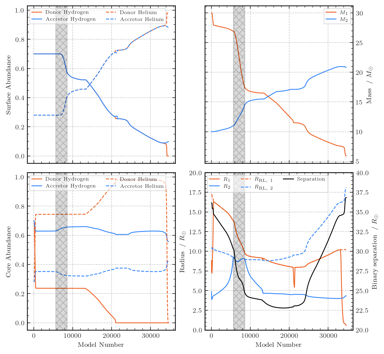
Figure 7: As for Figure 1, but indexed by model number across the entire evolutionary history of the binary. The donor’s radial contraction at $N\sim 21000$ is caused by hydrogen exhaustion in the core (as more energy is released by gravitational collapse than nuclear fusion), akin to the hook on the HR diagram, and marked on Figure 5. Similarly, the contraction at $N\sim 34000$ is due to helium exhaustion, and the development of the CO core.

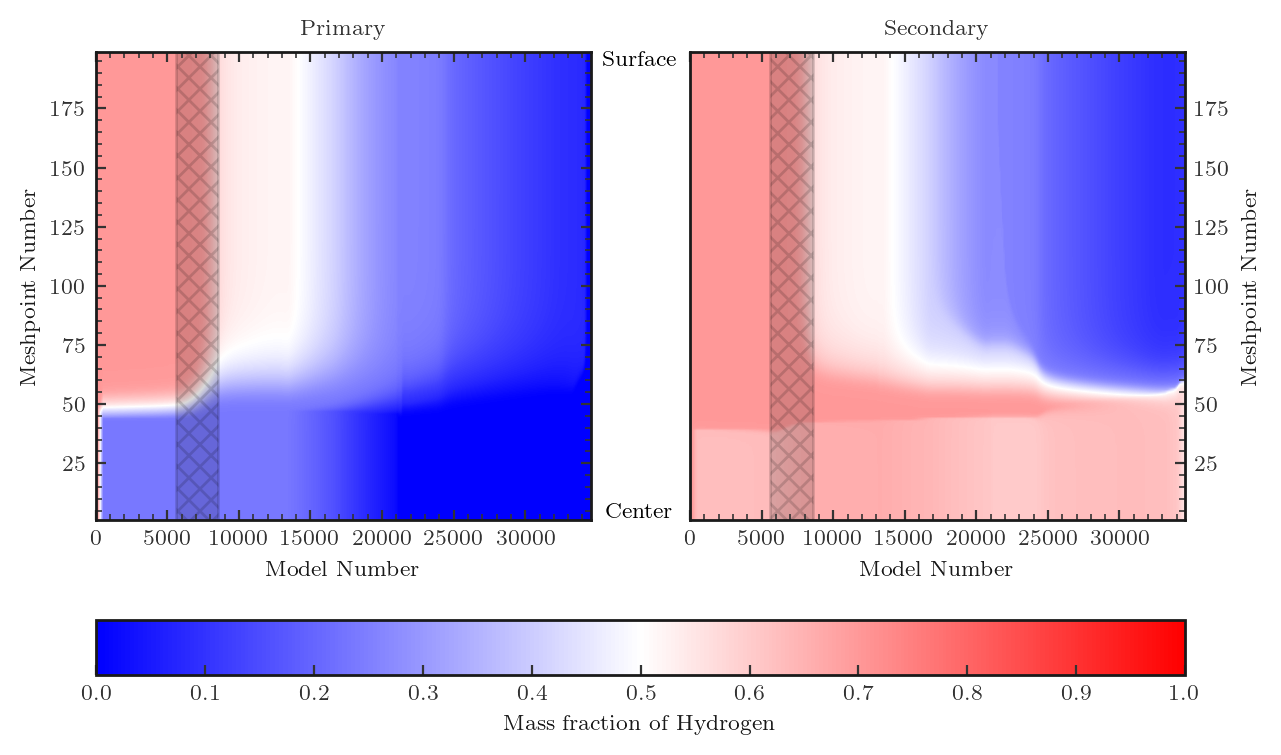
(a) Hydrogen profile

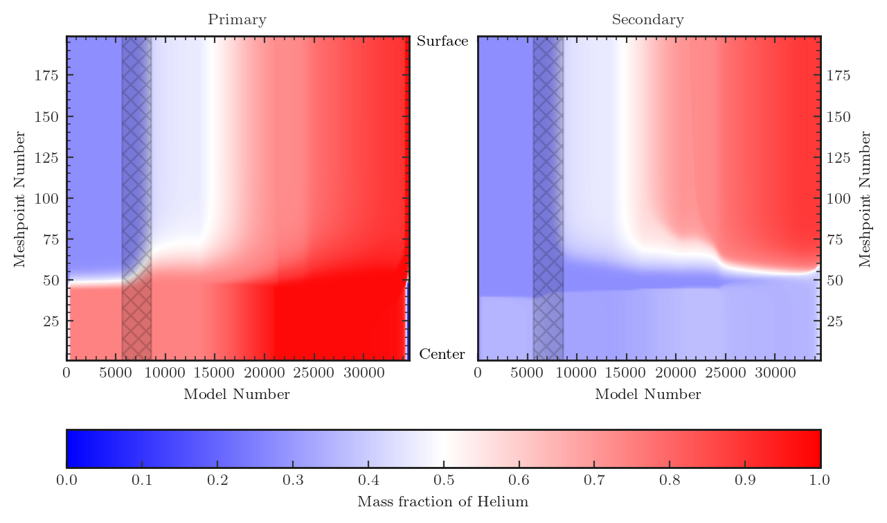
(b) Helium profile

Figure 8: The interior composition evolution of both stars in a $30+10\text{\,}\mathrm{M_{\odot}}$ binary with an initial period of $\log~{}P=$0.6\text{\,}\mathrm{d}$$. In both plots, the region where both stars fill their Roche lobe is denoted by the shaded black region.

Appendix B Model data at key evolutionary stages

Table 2 shows key binary and stellar data at different stages of the lifetime of the binary. The table labels correspond to the stages shown in Figure 4, and the lexicographic ordering of the labels corresponds to advancing in the evolution of the star.

			RLOF – Star 1		RLOF – Star 2
		$t=0$ (a)	Begin (b)	End (e)	Begin (c)	End (d)
Donor	$M~{}/~{}\unit{}$	30.00	27.93	7.56	26.91	17.43
	$R~{}/~{}\unit{}$	8.82	16.32	10.20	13.88	9.76
	$\log L~{}/~{}\unit{}$	5.07	5.30	5.25	5.16	4.94
	$X_{\text{surf}}$	0.70	0.70	0.09	0.70	0.57
	$Y_{\text{surf}}$	0.28	0.28	0.89	0.28	0.41
Accretor	$M~{}/~{}\unit{}$	10.00	9.99	20.97	11.00	14.57
	$R~{}/~{}\unit{}$	4.87	4.36	4.02	9.23	8.98
	$\log L~{}/~{}\unit{}$	3.73	3.81	4.89	4.90	5.06
	$X_{\text{surf}}$	0.70	0.70	0.09	0.70	0.57
	$Y_{\text{surf}}$	0.28	0.28	0.89	0.28	0.41
Binary	$P_{\text{bin}}~{}/~{}\unit{}$	3.98	3.85	4.41	3.14	2.52
	$a~{}/~{}\unit{}$	36.14	34.74	34.56	30.28	24.71
	Age /	0.00	4707.16	6450.23	4712.75	4716.42

(a) Variable composition accretion

			RLOF – Star 1		RLOF – Star 2
		$t=0$ (a)	Begin (b)	End (e)	Begin (c)	End (d)
Donor	$M~{}/~{}\unit{}$	30.00	27.93	7.57	26.91	17.27
	$R~{}/~{}\unit{}$	8.82	16.32	10.15	13.88	9.77
	$\log L~{}/~{}\unit{}$	5.07	5.30	5.25	5.16	4.98
	$X_{\text{surf}}$	0.70	0.70	0.09	0.70	0.57
	$Y_{\text{surf}}$	0.28	0.28	0.89	0.28	0.42
Accretor	$M~{}/~{}\unit{}$	10.00	9.99	20.77	11.00	14.52
	$R~{}/~{}\unit{}$	4.87	4.36	6.53	9.23	9.02
	$\log L~{}/~{}\unit{}$	3.73	3.81	4.73	4.90	4.95
	$X_{\text{surf}}$	0.70	0.70	0.70	0.70	0.70
	$Y_{\text{surf}}$	0.28	0.28	0.28	0.28	0.28
Binary	$P_{\text{bin}}~{}/~{}\unit{}$	3.98	3.85	4.38	3.14	2.54
	$a~{}/~{}\unit{}$	36.14	34.74	34.33	30.28	24.78
	Age /	0.00	4707.16	6448.11	4712.75	4716.70

(b) Non-variable accretion

Table 2: The key evolutionary parameters of both stars and the binary configuration at five critical points: the initial parameters, and the beginning and ends of both epochs of RLOF. All values are rounded to 2 decimal places. The letter in parentheses represents which segment of 4(a) (for 2(a)) or 4(b) (for 2(b)) the abundances are given in. These same markings represent the stages denoted on the donor in Figure 1.

References

- Bavera et al. (2020) Bavera S. S., et al., 2020, A&A, 635, A97
- Beasor et al. (2023) Beasor E. R., Smith N., Andrews J. E., 2023, The Astrophysical Journal, 952, 113
- Bestenlehner et al. (2020) Bestenlehner J. M., et al., 2020, Monthly Notices of the Royal Astronomical Society, 499, 1918
- Boffin & Jorissen (1988) Boffin H. M. J., Jorissen A., 1988, Astronomy and Astrophysics, 205, 155
- Bondi & Hoyle (1944) Bondi H., Hoyle F., 1944, Monthly Notices of the Royal Astronomical Society, 104, 273
- Bouret et al. (2013) Bouret J. C., Lanz T., Martins F., Marcolino W. L. F., Hillier D. J., Depagne E., Hubeny I., 2013, Astronomy and Astrophysics, 555, A1
- Cantiello et al. (2007) Cantiello M., Yoon S. C., Langer N., Livio M., 2007, Astronomy and Astrophysics, 465, L29
- Chen & Han (2004) Chen X., Han Z., 2004, Monthly Notices of the Royal Astronomical Society, 355, 1182
- Davis et al. (2013) Davis P. J., Siess L., Deschamps R., 2013, Astronomy & Astrophysics, 556, A4
- Delgado & Thomas (1981) Delgado A. J., Thomas H. C., 1981, Astronomy and Astrophysics, 96, 142
- Dorn-Wallenstein et al. (2023) Dorn-Wallenstein T. Z., Neugent K. F., Levesque E. M., 2023, The Astrophysical Journal, 959, 102
- Dorozsmai & Toonen (2024) Dorozsmai A., Toonen S., 2024, Monthly Notices of the Royal Astronomical Society, 530, 3706
- Drout et al. (2023) Drout M. R., Götberg Y., Ludwig B. A., Groh J. H., de Mink S. E., O’Grady A. J. G., Smith N., 2023, Science, 382, 1287
- Dutta & Klencki (2023) Dutta D., Klencki J., 2023, On the evolutionary nature of puffed-up stripped star binaries and their occurrence in stellar populations (arXiv:2312.12658), doi:10.48550/arXiv.2312.12658
- Eggenberger et al. (2010) Eggenberger P., et al., 2010, Astronomy & Astrophysics, 519, A116
- Eggleton (1971) Eggleton P. P., 1971, Monthly Notices of the Royal Astronomical Society, 151, 351
- Eggleton (1983) Eggleton P. P., 1983, The Astrophysical Journal, 268, 368
- Ekström et al. (2012) Ekström S., et al., 2012, Astronomy & Astrophysics, 537, A146
- Eldridge & Maund (2016) Eldridge J. J., Maund J. R., 2016, MNRAS, 461, L117
- Eldridge & Stanway (2012) Eldridge J. J., Stanway E. R., 2012, Monthly Notices of the Royal Astronomical Society, 419, 479
- Eldridge & Stanway (2022) Eldridge J. J., Stanway E. R., 2022, Annual Review of Astronomy and Astrophysics, 60, 455
- Eldridge & Tout (2004a) Eldridge J. J., Tout C. A., 2004a, MNRAS, 348, 201
- Eldridge & Tout (2004b) Eldridge J. J., Tout C. A., 2004b, MNRAS, 353, 87
- Eldridge et al. (2011) Eldridge J. J., Langer N., Tout C. A., 2011, MNRAS, 414, 3501
- Eldridge et al. (2013) Eldridge J. J., Fraser M., Smartt S. J., Maund J. R., Crockett R. M., 2013, MNRAS, 436, 774
- Eldridge et al. (2017) Eldridge J. J., Stanway E. R., Xiao L., McClelland L. A. S., Taylor G., Ng M., Greis S. M. L., Bray J. C., 2017, Publications of the Astronomical Society of Australia, 34
- Fuller & Lu (2022) Fuller J., Lu W., 2022, MNRAS, 511, 3951
- Ghodla et al. (2023) Ghodla S., Eldridge J. J., Stanway E. R., Stevance H. F., 2023, MNRAS, 518, 860
- Götberg et al. (2017) Götberg Y., de Mink S. E., Groh J. H., 2017, A&A, 608, A11
- Graur et al. (2017) Graur O., Bianco F. B., Modjaz M., Shivvers I., Filippenko A. V., Li W., Smith N., 2017, The Astrophysical Journal, 837, 121
- Grevesse & Noels (1993) Grevesse N., Noels A., 1993, in Prantzos N., Vangioni-Flam E., Casse M., eds, Origin and Evolution of the Elements. pp 15–25
- Gräfener et al. (2002) Gräfener G., Koesterke L., Hamann W. R., 2002, Astronomy and Astrophysics, 387, 244
- Götberg et al. (2018) Götberg Y., de Mink S. E., Groh J. H., Kupfer T., Crowther P. A., Zapartas E., Renzo M., 2018, Astronomy and Astrophysics, 615, A78
- Götberg et al. (2023) Götberg Y., et al., 2023, The Astrophysical Journal, 959, 125
- Hamann & Gräfener (2003) Hamann W. R., Gräfener G., 2003, Astronomy and Astrophysics, 410, 993
- Herrero et al. (1992) Herrero A., Kudritzki R. P., Vilchez J. M., Kunze D., Butler K., Haser S., 1992, Astronomy and Astrophysics, 261, 209
- Hirai et al. (2018) Hirai R., Podsiadlowski P., Yamada S., 2018, The Astrophysical Journal, 864, 119
- Hunter et al. (2008) Hunter I., et al., 2008, The Astrophysical Journal, 676, L29
- Hurley et al. (2002) Hurley J. R., Tout C. A., Pols O. R., 2002, MNRAS, 329, 897
- Hut (1981) Hut P., 1981, Astronomy and Astrophysics, 99, 126
- Kippenhahn et al. (1980) Kippenhahn R., Ruschenplatt G., Thomas H. C., 1980, Astronomy and Astrophysics, 91, 175
- Klencki et al. (2021) Klencki J., Nelemans G., Istrate A. G., Chruslinska M., 2021, Astronomy & Astrophysics, 645, A54
- Lamers et al. (1995) Lamers H. J. G. L. M., Snow T. P., Lindholm D. M., 1995, The Astrophysical Journal, 455, 269
- Landri et al. (2024) Landri C., Ricker P. M., Renzo M., Rau S., Vigna-Gómez A., 2024, arXiv, p. arXiv:2407.15932
- Langer (2012) Langer N., 2012, Annual Review of Astronomy and Astrophysics, 50, 107
- Laplace et al. (2021) Laplace E., Justham S., Renzo M., Götberg Y., Farmer R., Vartanyan D., de Mink S. E., 2021, A&A, 656, A58
- Lau et al. (2024) Lau M. Y. M., Hirai R., Mandel I., Tout C. A., 2024, The Astrophysical Journal, 966, L7
- Law-Smith et al. (2020) Law-Smith J. A. P., et al., 2020, Successful Common Envelope Ejection and Binary Neutron Star Formation in 3D Hydrodynamics, doi:10.48550/arXiv.2011.06630, https://ui.adsabs.harvard.edu/abs/2020arXiv201106630L
- Leung (1989) Leung K. C., 1989, in Batten A. H., ed., Algols. Springer Netherlands, Dordrecht, pp 279–288, doi:10.1007/978-94-009-2413-0_24
- Maeder (1990) Maeder A., 1990, Astronomy and Astrophysics Supplement Series, 84, 139
- Markova et al. (2018) Markova N., Puls J., Langer N., 2018, Astronomy and Astrophysics, 613, A12
- Massey et al. (2009) Massey P., Zangari A. M., Morrell N. I., Puls J., DeGioia-Eastwood K., Bresolin F., Kudritzki R.-P., 2009, The Astrophysical Journal, 692, 618
- Massey et al. (2013) Massey P., Neugent K. F., Hillier D. J., Puls J., 2013, The Astrophysical Journal, 768, 6
- Massey et al. (2023) Massey P., Neugent K. F., Morrell N. I., 2023, The Astrophysical Journal, 947, 77
- McEvoy et al. (2015) McEvoy C. M., et al., 2015, Astronomy and Astrophysics, 575, A70
- Menon et al. (2024) Menon A., et al., 2024, The Astrophysical Journal, 963, L42
- Nugis & Lamers (2000) Nugis T., Lamers H. J. G. L. M., 2000, A&A, 360, 227
- Packet (1981) Packet W., 1981, Astronomy and Astrophysics, 102, 17
- Paczynski (1991) Paczynski B., 1991, ApJ, 370, 597
- Pedersen et al. (2021) Pedersen M. G., et al., 2021, Nature Astronomy, 5, 715
- Podsiadlowski (2017) Podsiadlowski P., 2017, in Alsabti A. W., Murdin P., eds, , Handbook of Supernovae. p. 635, doi:10.1007/978-3-319-21846-5_123
- Pols (1994) Pols O. R., 1994, Astronomy and Astrophysics, 290, 119
- Popham & Narayan (1991) Popham R., Narayan R., 1991, ApJ, 370, 604
- Qin et al. (2018) Qin Y., Fragos T., Meynet G., Andrews J., Sørensen M., Song H. F., 2018, A&A, 616, A28
- Ramachandran et al. (2018) Ramachandran V., Hamann W. R., Hainich R., Oskinova L. M., Shenar T., Sander A. A. C., Todt H., Gallagher J. S., 2018, Astronomy and Astrophysics, 615, A40
- Renzo & Götberg (2021) Renzo M., Götberg Y., 2021, ApJ, 923, 277
- Renzo et al. (2023) Renzo M., Zapartas E., Justham S., Breivik K., Lau M., Farmer R., Cantiello M., Metzger B. D., 2023, ApJ, 942, L32
- Richards et al. (2023) Richards S. M., Eldridge J. J., Briel M. M., Stevance H. F., Willcox R., 2023, Monthly Notices of the Royal Astronomical Society, 522, 3972
- Sander et al. (2015) Sander A., Shenar T., Hainich R., Gímenez-García A., Todt H., Hamann W. R., 2015, Astronomy and Astrophysics, 577, A13
- Schneider et al. (2014) Schneider F. R. N., Langer N., de Koter A., Brott I., Izzard R. G., Lau H. H. B., 2014, Astronomy and Astrophysics, 570, A66
- Schneider et al. (2024) Schneider F. R. N., Podsiadlowski P., Laplace E., 2024, Astronomy & Astrophysics, 686, A45
- Sen et al. (2022) Sen K., et al., 2022, Astronomy and Astrophysics, 659, A98
- Smith & Tombleson (2015) Smith N., Tombleson R., 2015, Monthly Notices of the Royal Astronomical Society, 447, 598
- Smith et al. (2011) Smith N., Li W., Filippenko A. V., Chornock R., 2011, MNRAS, 412, 1522
- Smith et al. (2012) Smith N., Mauerhan J. C., Silverman J. M., Ganeshalingam M., Filippenko A. V., Cenko S. B., Clubb K. I., Kandrashoff M. T., 2012, Monthly Notices of the Royal Astronomical Society, 426, 1905
- Smith et al. (2018) Smith N., Götberg Y., de Mink S. E., 2018, Monthly Notices of the Royal Astronomical Society, 475, 772
- Soberman et al. (1997) Soberman G. E., Phinney E. S., van den Heuvel E. P. J., 1997, Astronomy and Astrophysics, 327, 620
- Stancliffe & Eldridge (2009) Stancliffe R. J., Eldridge J. J., 2009, Monthly Notices of the Royal Astronomical Society, 396, 1699
- Stancliffe et al. (2005) Stancliffe R. J., Lugaro M., Ugalde C., Tout C. A., Görres J., Wiescher M., 2005, Monthly Notices of the Royal Astronomical Society, 360, 375
- Stanway et al. (2016) Stanway E. R., Eldridge J. J., Becker G. D., 2016, MNRAS, 456, 485
- Stevance et al. (2023) Stevance H. F., Eldridge J. J., Stanway E. R., Lyman J., McLeod A. F., Levan A. J., 2023, Nature Astronomy, 7, 444
- Ulrich (1972) Ulrich R. K., 1972, The Astrophysical Journal, 172, 165
- De Donder & Vanbeveren (1998) De Donder E., Vanbeveren D., 1998, A&A, 333, 557
- de Jager et al. (1988) de Jager C., Nieuwenhuijden H., van der Hucht K. A., 1988, Bulletin d’Information du Centre de Donnees Stellaires, 35, 141
- de Loore & Vanbeveren (1994) de Loore C., Vanbeveren D., 1994, Astronomy and Astrophysics, 292, 463
- de Loore & Vanbeveren (1995) de Loore C., Vanbeveren D., 1995, Astronomy and Astrophysics, 304, 220
- de Mink et al. (2007) de Mink S. E., Pols O. R., Hilditch R. W., 2007, Astronomy & Astrophysics, 467, 1181
- de Mink et al. (2013) de Mink S. E., Langer N., Izzard R. G., Sana H., de Koter A., 2013, The Astrophysical Journal, 764, 166
- Vanbeveren et al. (1998) Vanbeveren D., De Loore C., Van Rensbergen W., 1998, The Astronomy and Astrophysics Review, 9, 63
- Vink et al. (2001) Vink J. S., de Koter A., Lamers H. J. G. L. M., 2001, Astronomy and Astrophysics, 369, 574
- Wagg et al. (2024) Wagg T., Johnston C., Bellinger E. P., Renzo M., Townsend R., Mink S. E. d., 2024, Astronomy & Astrophysics, 687, A222
- Wellstein et al. (2001) Wellstein S., Langer N., Braun H., 2001, A&A, 369, 939
- Xiao et al. (2018) Xiao L., Stanway E. R., Eldridge J. J., 2018, MNRAS, 477, 904
- Zahn (1977) Zahn J. P., 1977, Astronomy and Astrophysics, 57, 383