Embedding Safety into RL: A New Take on Trust Region Methods

Abstract

Reinforcement Learning (RL) agents are able to solve a wide variety of tasks but are prone to producing unsafe behaviors. Constrained Markov Decision Processes (CMDPs) provide a popular framework for incorporating safety constraints. However, common solution methods often compromise reward maximization by being overly conservative or allow unsafe behavior during training. We propose Constrained Trust Region Policy Optimization (C-TRPO), a novel approach that modifies the geometry of the policy space based on the safety constraints and yields trust regions composed exclusively of safe policies, ensuring constraint satisfaction throughout training. We theoretically study the convergence and update properties of C-TRPO and highlight connections to TRPO, Natural Policy Gradient (NPG), and Constrained Policy Optimization (CPO). Finally, we demonstrate experimentally that C-TRPO significantly reduces constraint violations while achieving competitive reward maximization compared to state-of-the-art CMDP algorithms.

1 Introduction

Reinforcement Learning (RL) has emerged as a highly successful paradigm in machine learning for solving sequential decision and control problems, with policy gradient (PG) algorithms as a popular approach (Williams, 1992; Sutton et al., 1999; Konda & Tsitsiklis, 1999). Policy gradients are especially appealing for high-dimensional continuous control because they can be easily extended to function approximation. Due to their flexibility and generality, there has been significant progress in enhancing PGs to work robustly with deep neural network-based approaches. Variants of natural policy gradient methods such as Trust Region Policy Optimization (TRPO) and Proximal Policy Optimization (PPO) are among the most widely used general-purpose reinforcement learning algorithms (Schulman et al., 2017a; b).

While flexibility makes PGs popular among practitioners, it comes at a price: the policy is free to explore any behavior during training, which poses substantial risk for applying such methods to real-world problems. Many methods have been introduced to improve the safety of policy gradients, often based on the Constrained Markov Decision Process (CMDP) formulation. However, existing methods are either limited in their ability to ensure minimal constraint violations during training or do so by severely limiting the agent’s performance.

This work introduces a simple strategy that can be used alongside trust-region-based safe policy gradient approaches to improve their constraint satisfaction throughout training, without sacrificing performance. We propose a novel family of policy divergences inspired by barrier function methods in optimization and safe control. These improve constraint satisfaction by altering the policy geometry to yield trust regions consisting exclusively of safe policies.

This approach is motivated by the observation that TRPO and related methods base their trust region on the state-average Kullback-Leibler (KL) divergence. It can be derived as the Bregman divergence induced by the negative conditional entropy on the space of state-action occupancies, as shown by Neu et al. (2017). The main insight of the present work is that safer trust regions can be derived by altering this function to incorporate the cost constraints. The resulting divergence is skewed away from the constraint surface, which is achieved by augmenting the negative conditional entropy by another convex barrier-like function. Manipulating the policy divergence in this way allows us to obtain a provably safe trust region-based policy optimization algorithm that retains most of TRPO’s mechanisms and guarantees, simplifying existing methods, while achieving competitive returns with less constraint violations throughout training.

Related work

Classic solution methods for CMDPs rely on linear programming techniques, see Altman (1999). However, LP-based approaches struggle to scale, making them unsuitable for high-dimensional or continuous control problems. While there are numerous works on CMDPs, in this section, we focus on model-free, direct policy optimization methods. For example, model-based approaches, like those popularized by Berkenkamp et al. (2017), usually provide stricter guarantees, but tend to be less general.

Penalty methods are a widely adopted approach, where the optimization problem is reformulated as a weighted objective that balances rewards and penalties for constraint violations. This is often motivated by Lagrangian duality, where the penalty coefficient is interpreted as the dual variable. Learning the coefficient with stochastic gradient descent presents a popular baseline (Achiam et al., 2017; Ray et al., 2019; Chow et al., 2019; Stooke et al., 2020). However, a naively tuned Lagrange multiplier may not work well in practice due to oscillations and overshoot. To address this issue, Stooke et al. (2020) apply PID control to tune the dual variable during training, which achieves less oscillations around the constraint and faster convergence to a feasible policy, see also Sohrabi et al. (2024). Methods such as P3O (Zhang et al., 2022), IPO (Liu et al., 2021), and those using (smoothed) log-barriers (Usmanova et al., 2024; Zhang et al., 2024; Ni & Kamgarpour, 2024; Dey et al., 2024) propose such weighted penalty-based policy optimization objectives from practical considerations. However, working with an explicit penalty introduces a bias and produces suboptimal policies concerning the original constrained MDP.

Our approach is closely related to trust region methods, particularly Constrained Policy Optimization (CPO) (Achiam et al., 2017), which extends TRPO by intersecting the trust region with the set of safe policies to ensure safety throughout training. While CPO offers certain guarantees on constraint satisfaction, it often leads to oscillations near the constraint surface due to cost advantage estimation errors. To address this, Yang et al. (2020) proposed Projection-based CPO (PCPO), which projects onto the safe policy space between updates. However, PCPO can significantly hinder reward maximization in practice.

Contributions

We summarize our contributions as follows:

• In Section 3, we introduce a modified policy divergence such that every trust region consists of only safe policies. We introduce an idealized TRPO update based on the modified divergence (C-TRPO), an approximate version of C-TRPO for deep function approximation, and a corresponding natural gradient method (C-NPG).

• We provide an efficient implementation of the proposed approximate C-TRPO method, see Section 3.2, which comes with a minimal overhead compared to TRPO (up to the estimation of the expected cost) and no overhead compared to CPO. We demonstrate experimentally that C-TRPO yields competitive returns with smaller constraint violations compared to common safe policy optimization algorithms, see Section 5.

• In Section 4, we introduce C-TRPO’s improvement guarantees and contrast to TRPO and CPO. Further, we show that the C-NPG method is the continuous time limit of C-TRPO and provides global convergence guarantees towards the optimal safe policy; this is in contrast to penalization or barrier methods, which introduce a bias

2 Background

We consider the infinite-horizon discounted constrained Markov decision process (CMDP) and refer the reader to Altman (1999) for a general treatment. The CMDP is given by the tuple $(\mathcal{S},\mathcal{A},P,r,\mu,\gamma,\mathcal{C})$, where $\mathcal{S}$ and $\mathcal{A}$ are the finite state-space and action-space respectively. Further, $P\colon\mathcal{S}\times\mathcal{A}\rightarrow\Delta_{\mathcal{S}}$ is the transition kernel, $r\colon\mathcal{S}\times\mathcal{A}\rightarrow\mathbb{R}$ is the reward function, $\mu\in\Delta_{\mathcal{S}}$ is the initial state distribution at time $t=0$, and $\gamma\in[0,1)$ is the discount factor. The space $\Delta_{\mathcal{S}}$ is the set of categorical distributions over $\mathcal{S}$. Further, define the constraint set $\mathcal{C}=\{(c_{i},b_{i})\}_{i=1}^{m}$, where $c_{i}\colon\mathcal{S}\times\mathcal{A}\to\mathbb{R}$ are the cost functions and $b_{i}\in\mathbb{R}$ are the cost thresholds.

An agent interacts with the CMDP by selecting a policy $\pi\in\Pi$ from the set of all Markov policies, i.e. an element from the Cartesian product of $|\mathcal{S}|$ probability simplicies on $\mathcal{A}$. Given such a policy $\pi$, the value functions $V_{r}^{\pi},V_{c_{i}}^{\pi}\colon\mathcal{S}\to\mathbb{R}$, action-value functions $Q_{r}^{\pi},Q_{c_{i}}^{\pi}\colon\mathcal{S}\times\mathcal{A}\to\mathbb{R}$, and advantage functions $A_{r}^{\pi},A_{c}^{\pi}\colon\mathcal{S}\times\mathcal{A}\to\mathbb{R}$ associated with the reward $r$ and the $i$-th cost $c_{i}$ are defined as

$$V_{f}^{\pi}(s)\coloneqq(1-\gamma)\,\mathbb{E}_{\pi}\left[\sum_{t=0}^{\infty}\gamma^{t}f(s_{t},a_{t})\Big{|}s_{0}=s\right],$$

where the function $f$ is either $r$ or $c_{i}$, and the expectations are taken over trajectories of the Markov process resulting from starting at $s$ and following policy $\pi$ and analogously

$$Q_{f}^{\pi}(s,a)\coloneqq(1-\gamma)\,\mathbb{E}_{\pi}\left[\sum_{t=0}^{\infty}\gamma^{t}f(s_{t},a_{t})\Big{|}s_{0}=s,a_{0}=a\right]\text{ and }A_{f}^{\pi}(s,a)\coloneqq Q_{f}^{\pi}(s,a)-V_{f}^{\pi}(s).$$

The goal is to solve the following constrained optimization problem

$$\text{maximize}_{\pi\in\Pi}\;V_{r}^{\pi}(\mu)\quad\text{subject to}\quad V_{c_{i}}^{\pi}(\mu)\leq b_{i}\quad\text{for all }i=1,\dots,m,$$ (1)

where $V_{f}^{\pi}(\mu)$ are the expected values under the initial state distribution $V_{f}^{\pi}(\mu)\coloneqq\mathbb{E}_{s\sim\mu}[V_{f}^{\pi}(s)].$ We will also write $V_{f}^{\pi}=V_{f}^{\pi}(\mu)$, and omit the explicit dependence on $\mu$ for convenience, and we write $V_{f}(\pi)$ when we want to emphasize its dependence on $\pi$. We denote the set of safe policies by $\Pi_{\operatorname{safe}}=\bigcap_{i=1}^{m}\{\pi:V_{c_{i}}(\pi)\leq b_{i}\}$ and always assume that it is nontrivial.

The Dual Linear Program for CMDPs

Any stationary policy $\pi$ induces a discounted state-action (occupancy) measure $d_{\pi}\in\Delta_{\mathcal{S}\times\mathcal{A}}$, indicating the relative frequencies of visiting a state-action pair, discounted by how far the event lies in the future. This probability measure is defined as

$$d_{\pi}(s,a)\coloneqq(1-\gamma)\sum_{t=0}^{\infty}\gamma^{t}\mathbb{P}_{\pi}(s_{t}=s)\pi(a|s),$$ (2)

where $\mathbb{P}_{\pi}(s_{t}=s)$ is the probability of observing the environment in state $s$ at time $t$ given the agent follows policy $\pi$. For finite MDPs, it is well-known that maximizing the expected discounted return can be expressed as the linear program

$$\operatorname{maximize}_{d}\,r^{\top}d\quad\text{subject to }d\in\mathscrsfs{D},$$

where $\mathscrsfs{D}$ is the set of feasible state-action measures, which form a polytope (Kallenberg, 1994). Analogously to an MDP, the discounted cost CMPD can be expressed as the linear program

$$\begin{split}\text{maximize}_{d}\;r^{\top}d\quad\text{subject to }d\in\mathscrsfs{D}_{\operatorname{safe}},\end{split}$$ (3)

where $\mathscrsfs{D}_{\operatorname{safe}}=\bigcap_{i=1}^{m}\left\{d:c_{i}^{\top}d\leq b_{i}\right\}\cap\mathscrsfs{D}$ is the safe occupancy set, see Figure 4 in Appendix A.

Information Geometry of Policy Optimization

Among the most successful policy optimization schemes are natural policy gradient (NPG) methods or variants thereof, such as trust-region and proximal policy optimization (TRPO and PPO, respectively). These methods assume a convex geometry and corresponding Bregman divergences in the state-action polytope, where we refer to Neu et al. (2017); Müller & Montúfar (2023) for a more detailed discussion.

In general, a trust region update is defined as

$$\pi_{k+1}\in\operatorname*{arg\,max}_{\pi\in\Pi}\mathbb{A}_{r}^{\pi_{k}}(\pi)\quad\text{ sbj. to }D_{\Phi}(d_{\pi_{k}}||d_{\pi})\leq\delta,$$ (4)

where $D_{\Phi}\colon\mathscrsfs{D}\times\mathscrsfs{D}\to\mathbb{R}$ is the Bregman divergence induced by a convex $\Phi\colon\operatorname{int}(\mathscrsfs{D})\rightarrow\mathbb{R}$, and

$$\mathbb{A}_{r}^{\pi_{k}}(\pi)=\mathbb{E}_{s,a\sim d_{\pi_{k}}}\left[\frac{\pi(a|s)}{\pi_{k}(a|s)}A_{r}^{\pi_{k}}(s,a)\right],$$ (5)

is called the policy advantage or surrogate advantage. We can interpret $\mathbb{A}$ as a surrogate optimization objective for the expected return. In particular, for a parameterized policy $\pi_{\theta}$, it holds that $\nabla_{\theta}\mathbb{A}_{r,\pi_{\theta_{k}}}(\pi_{\theta})|_{\theta=\theta_{k}}=\nabla_{\theta}V_{r}(\theta_{k})$, see Kakade & Langford (2002); Schulman et al. (2017a).

TRPO and the original NPG assume the same policy geometry (Kakade, 2001; Schulman et al., 2017a), since they employ an identical Bregman divergence

$$D_{\operatorname{K}}(d_{\pi_{1}}||d_{\pi_{2}}) \coloneqq\sum_{s,a}d_{\pi_{1}}(s,a)\log\frac{\pi_{1}(a|s)}{\pi_{2}(a|s)}=\sum_{s}d_{\pi_{1}}(s)D_{\operatorname{KL}}(\pi_{1}(\cdot|s)||\pi_{2}(\cdot|s)).$$

We refer to $D_{\operatorname{K}}$ as the Kakade divergence and informally write $D_{\operatorname{K}}(\pi_{1},\pi_{2})\coloneqq D_{\operatorname{K}}(d_{\pi_{1}},d_{\pi_{2}})$. This divergence can be shown to be the Bregman divergence induced by the negative conditional entropy

$$\Phi_{\operatorname{K}}(d_{\pi})\coloneqq\sum_{s,a}d_{\pi}(s,a)\log\pi(a|s),$$ (6)

see Neu et al. (2017). It is well known that with a parameterized policy $\pi_{\theta}$, a linear approximation of $\mathbb{A}$ and a quadratic approximation of the Bregman divergence $D_{\operatorname{K}}$ at $\theta_{k}$, one obtains the natural policy gradient step given by

$$\theta_{k+1}=\theta_{k}+\epsilon_{k}G_{\operatorname{K}}(\theta_{k})^{+}\nabla_{\theta}V_{r}(\pi_{\theta_{k}}),$$ (7)

where $G_{\operatorname{K}}(\theta)^{+}$ denotes a pseudo-inverse of the generalized Fisher-information matrix of the policy with entries given by $G_{\operatorname{K}}(\theta)_{ij}=\partial_{\theta_{i}}d_{\theta}\nabla^{2}\Phi_{\operatorname{K}}(d_{\theta})\partial_{\theta_{j}}d_{\theta}$, see Schulman et al. (2017a); Müller & Montúfar (2023) and Section A.1 for more detailed discussions.

3 A Safe Geometry for Constrained MDPs

Existing approaches to CMDPs use a Lagrangian reformulation, projections onto the safe policy set, or penalization to approximately or exactly enforce the constraints. In addition, CPO is an adaptation of TRPO, where the trust region intersects with the set of safe policies. We take a similar approach to CPO but construct trust regions that are contained in the safe policy set by design, as illustrated in Figure 1. The main advantage of formulating a safe policy optimization algorithm as a trust region method is that it inherits TRPO’s update guarantees for both the reward as well as the constraints.

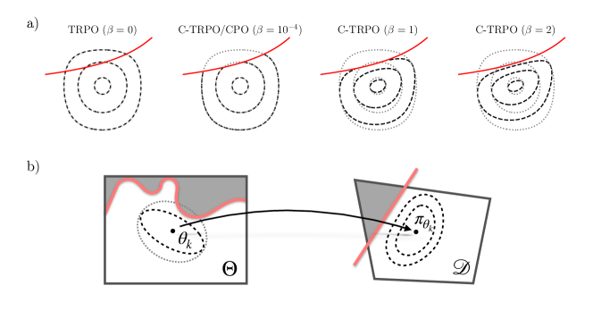
Figure 1: a) The constrained KL-divergence in policy space (dashed) centered at a point close to the constraint surface (red). TRPO’s trust region (dotted) for reference. For different choices of $\beta$, different algorithms are obtained (from left to right): TRPO ($\beta=1$), CPO ($\beta\searrow 0$), and the more conservative C-TRPO ($\beta=1$, $\beta=2$). b) The divergence is obtained by mapping the policy onto its occupancy measure on the state-action polytope, where a safe geometry can be defined using standard tools from convex optimization (safe region in white).

3.1 Safe Trust Regions and Constrained TRPO

To prevent the policy iterates from violating the constraints during optimization, we construct a mirror function for the safe occupancy set $\mathscrsfs{D}_{\operatorname{safe}}$ rather than the entire state-action polytope $\mathscrsfs{D}$. For this, we consider mirror functions of the following form.

$$\Phi_{\operatorname{C}}(d)\coloneqq\Phi_{\operatorname{K}}(d)+\sum_{i=1}^{m}\beta_{i}\phi(b_{i}-c_{i}^{\top}d),$$ (8)

where $\Phi_{\operatorname{K}}$ is the conditional entropy defined in Equation 6, and $\phi\colon\mathbb{R}_{>0}\to\mathbb{R}$ is a convex function with $\phi^{\prime}(x)\to+\infty$ for $x\searrow 0$. This ensures that $\Phi_{\operatorname{C}}\colon\operatorname{int}(\mathscrsfs{D}_{\textup{safe}})\to\mathbb{R}$ is strictly convex and has infinite curvature at the cost surface $b_{i}-c_{i}^{\top}d=0$, which means $\lVert\nabla\Phi_{\operatorname{C}}(d_{k})\rVert\to+\infty$, when $b_{i}-c_{i}^{\top}d_{k}\searrow 0$. Possible candidates for $\phi$ are $\phi(x)=-\log(x)$ and $\phi(x)=x\log(x)$ corresponding to a logarithmic barrier and entropy, respectively.

The Bregman divergence induced by $\Phi_{\operatorname{C}}$ is given by

$$D_{{\operatorname{C}}}(d_{1}||d_{2})=D_{\operatorname{K}}(d_{1}||d_{2})+\sum_{i=1}^{m}\beta_{i}D_{\phi_{i}}(d_{1}||d_{2}),$$ (9)

where

$$\begin{split}D_{\phi_{i}}(d_{1}||d_{2})=&\,\phi(b_{i}-V_{c_{i}}(\pi_{1}))-\phi(b_{i}-V_{c_{i}}(\pi_{2}))+\phi^{\prime}(b_{i}-V_{c_{i}}(\pi_{2}))(V_{c_{i}}(\pi_{1})-V_{c_{i}}(\pi_{2})).\end{split}$$ (10)

The corresponding trust-region scheme is given by

$$\pi_{k+1}\in\operatorname*{arg\,max}_{\pi\in\Pi}\mathbb{A}_{r}^{\pi_{k}}(\pi)\quad\text{ sbj. to }D_{\operatorname{C}}(d_{\pi_{k}}||d_{\pi})\leq\delta,$$ (11)

where $\mathbb{A}_{r}$ is defined in Equation 5 and we refer to this as constrained TRPO (C-TRPO).

Note the constraint is only satisfied if $d_{1},d_{2}\in\operatorname{int}(\mathscrsfs{D}_{\textup{safe}})$ and the divergence approaches $+\infty$ as $d_{2}$ approaches the boundary of the safe set. Thus, the trust region $\{d\in\mathscrsfs{D}:D_{\operatorname{C}}(d_{k}||d)\leq\delta\}$ is contained in the set of safe occupancy measures for any finite $\delta$. Further, we will show in Theorem 6 that $\operatorname{int}(\mathscrsfs{D}_{\textup{safe}})$ is invariant under the training dynamics of constrained natural policy gradients.

Analogously to the case of unconstrained TRPO the corresponding constrained natural policy gradient (C-NPG) scheme is given by

$$\theta_{k+1}=\theta_{k}+\epsilon_{k}G_{\operatorname{C}}(\theta_{k})^{+}\nabla V_{r}(\theta_{k}),$$ (12)

where $G_{\operatorname{C}}(\theta)^{+}$ denotes an arbitrary pseudo-inverse of $G_{\operatorname{C}}(\theta)_{ij}=\partial_{\theta_{i}}d_{\theta}^{\top}\nabla^{2}\Phi_{\operatorname{C}}(d_{\theta})\partial_{\theta_{j}}d_{\theta}$.

3.2 Implementation Details of C-TRPO

Algorithm 1 describes our implementation of C-TRPO, which either performs the constrained trust region update if the current policy is safe or minimizes the cost if the policy is unsafe.

In practice, the exact trust region update Equation 11 cannot be computed, and we rely on a similar implementation as the original TRPO method that estimates the divergence, uses a linear approximation of the surrogate objective and a quadratic approximation of the trust region. To aid in clarity, we focus on the case with a single constraint, but the results are easily extended to multiple constraints by summation of the individual constraint terms.

Algorithm 1 Constrained TRPO (C-TRPO); differences from TRPO in blue

1:  Input: Initial policy $\pi_{0}\in\Pi_{\theta}$, safety parameter $\beta>0$, recovery parameter $0<b_{\textsc{H}}\leq b$

2:  for $k=0,1,2,\ldots$ do

3:     Sample a set of trajectories following $\pi_{k}=\pi_{\theta_{k}}$

4:     if $\pi_{k}\in\Pi^{\textsc{H}}_{\operatorname{safe}}$ then

5:        $A\leftarrow A_{r}$; $D\leftarrow\bar{D}_{\operatorname{C}}=\bar{D}_{\operatorname{KL}}\color[rgb]{0,0,1}+\beta\bar{D}_{\operatorname{\Phi}}$ {Constrained trust region update}

6:     else

7:        $\color[rgb]{0,0,1}A\leftarrow A_{c}$; $D\leftarrow\bar{D}_{\operatorname{KL}}$ {Recovery}

8:     end if

9:     Compute $\pi_{k+1}$ using TRPO with $A$ as advantage estimate and with $D$ as policy divergence.

10:  end for

Surrogate Divergence

In practice, the exact constrained KL-Divergence $D_{\operatorname{C}}$ cannot be evaluated, because it depends on the cost-return of the optimized policy $V_{c}(\pi)$. However, we can approximate it locally around the policy of the $k$-th iteration, $\pi_{k}$, using a surrogate divergence. This surrogate can be expressed as a function of the policy cost advantage

$$\mathbb{A}_{c}^{\pi_{k}}(\pi)=\mathbb{E}_{d_{\pi_{k}}}\left[\frac{\pi(a|s)}{\pi_{k}(a|s)}A_{c}^{\pi_{k}}(s,a)\right],$$ (13)

which approximates $V_{c}(\pi)-V_{c}^{\pi_{k}}$ up to first order in the policy parameters (Kakade & Langford, 2002; Schulman et al., 2017a; Achiam et al., 2017).

Assume $\pi_{k}\in\Pi_{\operatorname{safe}}$ and define the constraint margin $\delta_{b}=b-V_{c}^{\pi_{k}}$, which is positive if $\pi_{k}\in\Pi_{\textsc{safe}}$. We propose the following approximate C-TRPO update

$$\pi_{k+1}=\operatorname*{arg\,max}_{\pi\in\Pi}\mathbb{A}_{r}^{\pi_{k}}(\pi)\quad\text{sbj. to }\bar{D}_{\operatorname{C}}(\pi||\pi_{k})\leq\delta$$ (14)

with the surrogate divergence $\bar{D}_{\operatorname{C}}(\pi||\pi_{k})=\bar{D}_{\mathrm{KL}}(\pi||\pi_{k})+\beta\bar{D}_{\phi}(\pi||\pi_{k})$, where

$$\bar{D}_{\phi}(\pi_{\theta}||\pi_{\theta_{k}})=\phi(\delta_{b}-\mathbb{A}_{c}^{\pi_{k}}(\pi))-\phi(\delta_{b})+\phi^{\prime}(\delta_{b})\mathbb{A}_{c}^{\pi_{k}}(\pi),$$ (15)

$$\bar{D}_{\mathrm{KL}}(\pi||\pi_{k})=\sum_{s\in\mathcal{S}}d_{\pi_{k}}(s)D_{\mathrm{KL}}(\pi||\pi_{k}).$$ (16)

Note that $\bar{D}_{\operatorname{K}}$ is not identical to the Kakade divergence $D_{\operatorname{K}}$ since the arguments of $D_{\operatorname{K}}$ are reversed. However, they are equivalent up to second order in the policy parameters, and $\bar{D}_{\operatorname{K}}$ is a common choice, where authors want to connect theoretical results to the practical TRPO algorithm as implemented by Schulman et al. (2017a), see Neu et al. (2017); Achiam et al. (2017).

The surrogate $\bar{D}_{\phi}$ is closely related to the Bregman divergence $D_{\phi}$. It is equivalent to the exact divergence, up to the substitution $(V_{c}(\pi)-V_{c}(\pi_{k}))\to\mathbb{A}_{c}^{\pi_{k}}(\pi)$, see Appendix B.1. The motivation and consequences of this substitution will be discussed in the next section. In the practical implementation, we estimate $\delta_{b}$, and the policy cost advantage from trajectory samples . using GAE-$\lambda$ estimates Schulman et al. (2018).

Quadratic Approximation

Practically, the C-TRPO optimization problem in Equation 14 is solved like traditional TRPO: the objective is approximated linearly, and the constraint is approximated quadratically in the policy parameters using automatic differentiation and the conjugate gradients algorithm. This leads to the policy parameter update

$$\theta_{k+1}=\theta_{k}+\alpha^{i}\sqrt{\frac{2\delta}{g^{\top}_{k}H^{-1}_{k}g_{k}}}\cdot H_{k}^{-1}g_{k},$$ (17)

where

$$g_{k}=\nabla_{\theta}\mathbb{A}_{c}^{\theta_{k}}(\pi_{\theta})|_{\theta=\theta_{k}}\quad\text{and }H_{k}=H(\theta_{k})=\nabla^{2}_{\theta}\bar{D}_{C}(\pi_{\theta}||\pi_{\theta_{k}})|_{\theta=\theta_{k}}$$ (18)

are finite sample estimates, and $H^{-1}g$ is approximated using conjugate gradients. The $\alpha^{i}\in[0,1]$ are the coefficients for backtracking line search, which ensures $\bar{D}_{\operatorname{C}}(\pi_{\theta}||\pi_{\theta_{k}})\leq\delta$.

Recall that although $\mathbb{A}_{r}$ is only a proxy of $V_{r}$, we have $\nabla_{\theta}\mathbb{A}_{r}^{\theta_{k}}(\theta)|_{\theta=\theta_{k}}=\nabla V_{r}(\theta_{k})$ and further, one can show that the Hessian

$$\nabla^{2}_{\theta}\bar{D}_{\operatorname{C}}(\theta||\hat{\theta})|_{\theta=\hat{\theta}} =G_{\operatorname{K}}(\theta_{k})+\beta\mathbf{J}_{\theta}V_{c}^{\hat{\theta}}(\theta)^{\top}\phi^{\prime\prime}(b-V_{c}^{\hat{\theta}}(\theta))\mathbf{J}_{\theta}V_{c}^{\hat{\theta}}(\theta),$$

is equivalent to the Gramian $G_{\operatorname{C}}(\theta_{k})$ of the C-NPG flow in Equation 23, see Section B.2.2. In particular, this shows that the approximate C-TRPO update can be interpreted as a natural policy gradient step with an adaptive step size, and that the surrogate and true constrained KL-divergences are equivalent up to second order in the parameters. This justifies the use of the surrogate divergence in C-TRPO implementations and motivates the discussion of the C-NPG flow in Section 4.2.

Recovery with Hysteresis

The iterate may still leave the safe policy set $\Pi_{\operatorname{safe}}$, either due to approximation errors of the divergence, or because we started outside the safe set. In this case, we perform a recovery step, where we only minimize the cost with TRPO as by Achiam et al. (2017). In tasks where the policy starts in the unsafe set, C-TRPO can get stuck at the cost surface. This is easily mitigated by including a hysteresis condition for returning to the safe set. If $\pi_{k-1}$ is the previous policy, then $\pi_{k}\in\Pi_{\textup{safe}}^{\textsc{H}}$ with $\Pi_{\textup{safe}}^{\textsc{H}}=\{\pi_{\theta}\in\Pi_{\theta}\text{ and }V_{c}(\pi_{\theta})\leq b_{\textsc{H}}\}$ where $b_{\textsc{H}}=b$ if $\pi_{k-1}\in\Pi_{\textup{safe}}^{\textsc{H}}$ and a user-specified fraction of $b$ otherwise.

Computational Complexity

The C-TRPO implementation adds no computational overhead compared to CPO, since $\bar{D}_{\phi}$ is just a function of the cost advantage estimate, and because it is simply added to the divergence of TRPO. Compared to TRPO, the cost value function must be approximated for cost advantage estimation.

4 Analysis of C-TRPO

Here, we provide a theoretical analysis of the updates of C-TRPO and study the convergence properties of the time-continuous version of the corresponding natural policy gradient method. All proofs are deferred to the appendix.

4.1 Analysis of the approximation

The practical C-TRPO algorithm is implemented using an approximation of the constrained KL-Divergence. The surrogate divergence $\bar{D}_{\operatorname{C}}$ introduced in Eq. 14 is identical to the theoretical Constrained KL-Divergence $D_{\operatorname{C}}$ introduced in Eq. 11 up to a mismatch between the policy advantage and the performance difference. This can be seen by rewriting $D_{\phi}$ as a function of the performance difference of the cost and replacing this expression by the policy cost advantage $\mathbb{A}_{c}^{{\pi_{2}}}$, see Appendix A. By the general theory of Bregman divergences, $\bar{D}_{\phi}$ is a (strictly) convex function of $\mathbb{A}_{c}^{\pi_{2}}$ if $\phi$ is (strictly) convex. For any suitable $\phi$ we have

$$\begin{split}\bar{D}_{\phi}(\pi_{1}||\pi_{2})&=\phi(\delta_{b}-\mathbb{A}_{c}^{{\pi_{2}}}(\pi_{1}))-\phi(\delta_{b})+\phi^{\prime}(\delta_{b})\mathbb{A}_{c}^{{\pi_{2}}}(\pi_{1}),\end{split}$$ (19)

where $\delta_{b}=b-V_{c}^{\pi_{2}}$, as before. The motivation for substituting $\mathbb{A}_{c}^{{\pi_{2}}}$ for the performance difference is their equivalence up to first order and that we can estimate $\mathbb{A}_{c}^{{\pi}}$ from samples of $d_{\pi}$. In addition, we can use the following bounds on the performance difference of two policies.

Theorem 1 (Performance Difference, Achiam et al. (2017)).

For any function $f(s,a)$, the following bounds hold

$$V_{f}(\pi_{1})-V_{f}(\pi_{2})\lesseqgtr\mathbb{A}^{\pi_{2}}_{f}(\pi_{1})\pm\frac{2\gamma\epsilon_{f}}{(1-\gamma)}\sqrt{\frac{1}{2}\mathbb{E}_{s\sim d_{\pi_{2}}}D_{\operatorname{KL}}(\pi_{1}(\cdot|s)||\pi_{2}(\cdot|s))}$$ (20)

where $\epsilon_{f}=\max_{s}|\mathbb{E}_{a\sim\pi_{1}}A^{\pi_{2}}_{f}(s,a)|$.

Proposition 1 can be interpreted as a bound on the error incurred by replacing the difference in returns $V_{f}(\pi_{1})-V_{f}(\pi)$ of any state-action function by its policy advantage $\mathbb{A}_{f}^{\pi_{2}}(\pi_{1})$.

Proposition 2 (C-TRPO reward update).

Set $\epsilon_{r}=\max_{s}|\mathbb{E}_{a\sim\pi_{k+1}}A_{r}^{\pi_{k}}(s,a)|$. The expected reward of a policy updated with C-TRPO is bounded from below by

$$V_{r}(\pi_{k+1})\geq V_{r}(\pi_{k})-\frac{\sqrt{2\delta}\gamma\epsilon_{r}}{1-\gamma}.$$ (21)

An analogous bound was established for CPO (Achiam et al., 2017). Constraint violation, however, behaves slightly differently for the two algorithms. To see this, we first establish a more concrete relation between C-TRPO and CPO. As $\beta\searrow 0$, the solution to Eq. 14 approaches the constraint surface in the worst case, and we recover the CPO optimization problem, see Figure 1.

Proposition 3.

The approximate C-TRPO update approaches the CPO update in the limit as $\beta\searrow 0$.

Further, C-TRPO is more conservative than CPO for any $\beta>0$ and as $\beta\to+\infty$ the updated is maximally constrained in the cost-increasing direction. This is formalized as follows.

Proposition 4 (C-TRPO worst-case constraint violation).

Consider $\Psi\colon[0,\delta_{b})\to[0,\infty)$ defined by $\Psi(x)=\phi(\delta_{b}-x)-\phi(\delta_{b})-\phi^{\prime}(\delta_{b})\cdot x$ such that $D_{\phi}(\pi||\pi_{k})=\Psi(\mathbb{A}_{c}^{\pi_{k}}(\pi))$. Further, set $\epsilon_{c}=\max_{s}|\mathbb{E}_{a\sim\pi_{k+1}}A_{c}^{\pi_{k}}(s,a)|$, and choose a strictly convex $\phi$. The worst-case constraint violation for C-TRPO is

$$V_{c}(\pi_{k+1})\leq V_{c}(\pi_{k})+\Psi^{-1}(\delta/\beta)+\frac{\sqrt{2\delta}\gamma\epsilon_{c}}{1-\gamma}.$$ (22)

Further, it holds that $\lim_{\beta\to+\infty}\Psi^{-1}(\delta/\beta)=0$ and $\Psi^{-1}(\delta/\beta)<b-V_{c}(\pi_{k})$ for all $\beta\in(0,\infty)$.

This result is analogous to the worst-case constraint violation for CPO (Achiam et al., 2017, Proposition 2), except that it depends on the choice of $\beta$ and is strictly less than that of CPO.

4.2 Invariance and Convergence of Constrained Natural Policy Gradients

It is well known that TRPO is equivalent to a natural policy gradient method with an adaptive step size, see also Section A.1. We study the time-continuous limit of C-TRPO and guarantee safety during training and global convergence.

In the context of constrained TRPO in Equation 11, we study the natural policy gradient flow

$$\partial_{t}\theta_{t}=G_{\operatorname{C}}(\theta_{t})^{+}\nabla V_{r}(\theta_{t}),$$ (23)

where $G_{\operatorname{C}}(\theta)^{+}$ denotes a pseudo-inverse of $G_{\operatorname{C}}(\theta)_{ij}=\partial_{\theta_{i}}d_{\theta}^{\top}\nabla^{2}\Phi_{\operatorname{C}}(d_{\theta})\partial_{\theta_{j}}d_{\theta}$ and $\theta\mapsto\pi_{\theta}$ is a differentiable policy parametrization. Moreover, we assume that $\theta\mapsto\pi_{\theta}$ is regular, that it is surjective and the Jacobian is of maximal rank everywhere. This assumption implies overparametrization but is satisfied for common models like tabular softmax, tabular escort, or expressive log-linear policy parameterizations (Agarwal et al., 2021a; Mei et al., 2020a; Müller & Montúfar, 2023).

We denote the set of safe parameters by $\Theta_{\operatorname{safe}}\coloneqq\{\theta\in\mathbb{R}^{p}:\pi_{\theta}\in\Pi_{\operatorname{safe}}\}$, which is non-convex in general and say that $\Theta_{\operatorname{safe}}$ is invariant under Equation 23 if $\theta_{0}\in\Theta_{\operatorname{safe}}$ implies $\theta_{t}\in\Theta_{\operatorname{safe}}$ for all $t$. Invariance is associated with safe control during optimization and is typically achieved via control barrier function methods (Ames et al., 2017; Cheng et al., 2019). We study the evolution of the state-action distributions $d_{t}=d^{\pi_{\theta_{t}}}$ as this allows us to employ the linear programming formulation of CMPDs and we obtain the following convergence guarantees.

Theorem 5 (Safety during training).

Assume that $\phi\colon\mathbb{R}_{>0}\to\mathbb{R}$ satisfies $\phi^{\prime}(x)\to+\infty$ for $x\searrow 0$ and consider a regular policy parameterization. Then the set $\Theta_{\operatorname{C}}$ is invariant under Equation 23.

A visualization of policies obtained by C-NPG for different safe initializations and varying choices of $\beta$ is shown in Figure 2 for a toy MDP. We see that for even small choices of $\beta$ the trajectories don’t cross the constraint surface and the updates become more conservative for larger choices of $\beta$.

Figure 2: Shown is the policy set $\Pi\cong[0,1]^{2}$ for an MDP with two states and two actions with a heatmap of the reward $V_{r}$; the constraint surface is shown in black with the safe policies below; optimization trajectories are shown for 10 safe initialization and for $\beta=0,10^{-4},10^{-2},1$.

Theorem 6.

Assume that $\phi^{\prime}(x)\to+\infty$ for $x\searrow 0$, set $V_{r,{\operatorname{C}}}^{\star}\coloneqq\max_{\pi\in\Pi_{\operatorname{safe}}}V_{r}(\pi)$ and denote the set of optimal constrained policies by $\Pi^{\star}_{\operatorname{safe}}=\{\pi\in\Pi_{\operatorname{safe}}:V_{r}(\pi)=V_{r,{\operatorname{C}}}^{\star}\}$, consider a regular policy parametrization and let $(\theta_{t})_{t\geq 0}$ solve Equation 23. It holds that $V_{r}(\pi_{\theta_{t}})\to V_{r,{\operatorname{C}}}^{\star}$ and

$$\lim_{t\to+\infty}\pi_{t}=\pi^{\star}_{\operatorname{safe}}=\arg\min\{D_{\operatorname{C}}(\pi^{\star},\pi_{0}):\pi^{\star}\in\Pi^{\star}_{\operatorname{safe}}\}.$$ (24)

In case of multiple optimal policies, Equation 24 identifies the optimal policy of the CMDP that the natural policy gradient method converges to as the projection of the initial policy $\pi_{0}$ to the set of optimal safe policies $\Pi^{\star}_{\operatorname{safe}}$ with respect to the constrained divergence $D_{\operatorname{C}}$. In particular, this implies that the limiting policy $\pi^{\star}_{\operatorname{safe}}$ satisfies as few constraints with equality as required to be optimal. To see this, note that $\Pi^{\star}_{\operatorname{safe}}$ forms a face of $\mathscrsfs{D}_{\operatorname{safe}}$ and that Bregman projections lie at the interior of faces (Müller et al., 2024, Lemma A.2) and hence satisfy as few linear constraints as required.

5 Computational Experiments

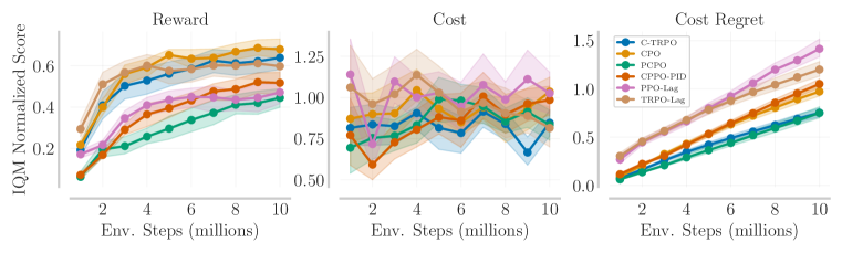
Figure 3: Comparison of safe policy optimization algorithms based on the Inter Quartile Mean across 5 seeds and 8 tasks. From left to right: episode return of the reward (PPO normalized), episode return of the cost (threshold normalized), and cumulative cost regret (CPO normalized).

Setup and main results

We benchmark C-TRPO against 5 common safe policy optimization algorithms (CPO, PCPO, CPPO-PID, PPO-Lag, TRPO-Lag) on 8 tasks (4 Navigation and 4 Locomotion) from the Safety Gymnasium (Ji et al., 2023) benchmark. For the C-TRPO implementation we fix the convex generator $\phi(x)=x\log(x)$, motivated by its superior performance in our experiments, see Appendix B.2.1, $b_{\textsc{H}}=0.8b$ and $\beta=1$ across all experiments.

We train each algorithm for 10 million environment steps and evaluate on 10 runs after training, see Table 1 in Appendix D. Furthermore, each algorithm is trained with 5 seeds, and the cost regret is monitored throughout training for every run. To get a better sense of the safety of the algorithms during training, we take an online learning perspective and include as a metric the strong cost regret (Efroni et al., 2020; Müller et al., 2024)

$$\textsc{CostReg}_{+}(K,c)\coloneqq\sum_{k=0}^{K-1}\left[V_{c}^{\pi_{k}}-b\right]_{+},$$ (25)

where $\left[x\right]_{+}=\max\{0,x\}$, and $K$ is the number of the training episodes.

We observe that C-TRPO is competitive with the leading algorithms of the benchmark in terms of expected return (CPO, TRPO-Lagrangian), see Figure 3. Furthermore, it achieves notably lower cost regret throughout training than the high-return algorithms, even comparable to the more conservative PCPO algorithm. In Figure 3, we visualize the interquartile mean (IQM) of normalized scores across training for expected returns of reward and cost and for the cost regret, including their stratified bootstrap confidence intervals (Agarwal et al., 2021b).

Discussion

For completeness, we also report environment-wise sample efficiency curves and evaluation performances in Appendix D.2. Our experiments reveal that the algorithm’s performance is closely tied to the accuracy of divergence estimation, which hinges on the precise estimation of the cost advantage and value functions. The safety parameter $\beta$ modulates the stringency with which C-TRPO satisfies the constraint, and can do so without limiting the expected return on most environments at least for $\beta\leq 1$, see Figure 6. For higher values, the expected return starts to degrade, partly due to $\bar{D}_{\phi}$ being relatively noisy compared to $\bar{D}_{\operatorname{KL}}$ and thus we recommend the choice $\beta=1$.

Further, we observe that constraint satisfaction is stable across different choices of cost threshold $b$, see Figure 7, and that in most environments, constraint violations seem to reduce as the algorithm converges, meaning that the regret flattens over time. This behavior suggests that the divergence estimation becomes increasingly accurate over time, potentially allowing C-TRPO to achieve sublinear regret. However, we leave regret analysis of the finite sample regime for future research.

We attribute the improved constraint satisfaction compared to CPO to a slowdown and reduction in the frequency of oscillations around the cost threshold, which mitigates overshoot behaviors that could otherwise violate constraints. The modified gradient preconditioner appears to deflect the parameter trajectory away from the constraint, see Figure 2. This effect may also be partially attributed to the hysteresis-based recovery mechanism, which helps smooth updates by leading the iterate away from the boundary of the safe set. Employing a hysteresis fraction $0<b_{\textsc{H}}<b$ might also be beneficial because divergence estimates tend to be more reliable for strictly safe policies. The effect of the choice of $b_{\textsc{H}}$ is visualized in Figure 8.

6 Conclusion and outlook

In this paper, we introduced C-TRPO and C-NPG, two novel methods for solving Constrained Markov Decision Processes (CMDPs). C-TRPO can be viewed as an extension or relaxation of Constrained Policy Optimization (CPO), from which a natural policy gradient method, C-NPG, is derived. C-TRPO represents a significant step toward safe, model-free reinforcement learning by integrating constraint handling directly into the geometry of the policy space. Meanwhile, C-NPG provides a provably safe natural policy gradient method for CMDPs, offering a foundational approach to direct policy optimization in constrained settings—similar to how NPG is a cornerstone in the theory of policy gradients for unconstrained MDPs.

However, there are several limitations to address. First, the divergence estimation remains challenging, and we did not investigate the properties of the finite sample estimates of the divergence. In addition, the CMDP framework may be somewhat limited in modeling safe exploration and control. Because CMDPs constrain the average cost return, it can be difficult to model trajectory-wise or state-wise safety constraints.

Several promising directions for future research remain open. One avenue is to combine these methods with model-based policy optimization to improve cost return estimates, or with policy mirror descent to improve computational efficiency, see e.g. Tomar et al. (2022). Future work could also investigate if the proposed methods can be formulated in a distributional RL setting, basing the divergence on the conditional value at risk (CVaR) of the cost, providing more reliable constraint satisfaction. Additionally, integrating the proposed divergence with other safe policy optimization algorithms that utilize trust regions, e.g. PCPO, could lead to stronger performance guarantees.

Overall, the proposed algorithms, C-TRPO and C-NPG, present a step forward in general-purpose CMDP algorithms and move us closer to deploying RL in high-stakes, real-world applications.

Acknowledgments

Appendix A Extended Background

We consider the infinite-horizon discounted Markov decision process (MDP), given by the tuple $(\mathcal{S},\mathcal{A},P,r,\mu,\gamma)$. Here, $\mathcal{S}$ and $\mathcal{A}$ are the finite state-space and action-space respectively. Further, $P\colon\mathcal{S}\times\mathcal{A}\rightarrow\Delta_{\mathcal{S}}$ is the transition kernel, $r\colon\mathcal{S}\times\mathcal{A}\rightarrow\mathbb{R}$ is the reward function, $\mu\in\Delta_{\mathcal{S}}$ is the initial state distribution at time $t=0$, and $\gamma\in[0,1)$ is the discount factor. The space $\Delta_{\mathcal{S}}$ is the set of categorical distributions over $\mathcal{S}$.

The Reinforcement Learning (RL) protocol is usually described as follows: At time $t=0$, an initial state $s_{0}$ is drawn from $\mu$. At each integer time-step $t$, the agent chooses an action according to it’s (stochastic) behavior policy $a_{t}\sim\pi(\cdot|s_{t})$. A reward $r_{t}=r(s_{t},a_{t})$ is given to the agent, and a new state $s_{t+1}\sim P(\cdot|s_{t},a_{t})$ is sampled from the environment. Given a policy $\pi$, the value function $V_{r}^{\pi}\colon\mathcal{S}\to\mathbb{R}$, action-value function $Q_{r}^{\pi}\colon\mathcal{S}\times\mathcal{A}\to\mathbb{R}$, and advantage function $A_{r}^{\pi}\colon\mathcal{S}\times\mathcal{A}\to\mathbb{R}$ associated with the reward $r$ are defined as

$$V_{r}^{\pi}(s)\coloneqq(1-\gamma)\,\mathbb{E}_{\pi}\left[\sum_{t=0}^{\infty}\gamma^{t}r(s_{t},a_{t})\Big{|}s_{0}=s\right],$$

$$Q_{r}^{\pi}(s,a)\coloneqq(1-\gamma)\,\mathbb{E}_{\pi}\left[\sum_{t=0}^{\infty}\gamma^{t}r(s_{t},a_{t})\Big{|}s_{0}=s,a_{0}=a\right]\text{ and }A_{r}^{\pi}(s,a)\coloneqq Q_{r}^{\pi}(s,a)-V_{r}^{\pi}(s).$$

where and the expectations are taken over trajectories of the Markov process resulting from starting at $s$ and following policy $\pi$. The goal is to

$$\text{maximize}_{\pi\in\Pi}\;V_{r}^{\pi}(\mu)$$ (26)

where $V_{r}^{\pi}(\mu)$ is the expected value under the initial state distribution $V_{r}^{\pi}(\mu)\coloneqq\mathbb{E}_{s\sim\mu}[V_{r}^{\pi}(s)].$ We will also write $V_{r}^{\pi}=V_{r}^{\pi}(\mu)$, and omit the explicit dependence on $\mu$ for convenience, and we write $V_{r}(\pi)$ when we want to emphasize its dependence on $\pi$.

The Dual Linear Program for MDPs

Any stationary policy $\pi$ induces a discounted state-action (occupancy) measure $d_{\pi}\in\Delta_{\mathcal{S}\times\mathcal{A}}$, indicating the relative frequencies of visiting a state-action pair, discounted by how far the visitation lies in the future. It is a probability measure defined as

$$d_{\pi}(s,a)\coloneqq(1-\gamma)\sum_{t=0}^{\infty}\gamma^{t}\mathbb{P}_{\pi}(s_{t}=s)\pi(a|s),$$ (27)

where $\mathbb{P}_{\pi}(s_{t}=s)$ is the probability of observing the environment in state $s$ at time $t$ given the agent follows policy $\pi$. For finite MDPs, it is well-known that maximizing the expected discounted return can be expressed as the linear program

$$\max_{d}\,r^{\top}d\quad\text{subject to }d\in\mathscrsfs{D},$$ (28)

where $\mathscrsfs{D}$ is the set of feasible state-action measures Feinberg & Shwartz (2012). This set is also known as the state-action polytope, defined by

$$\mathscrsfs{D}=\left\{d\in\mathbb{R}_{\geq 0}^{\mathcal{S}\times\mathcal{A}}:\ell_{s}(d)=0\text{ for all }s\in\mathcal{S}\right\},$$

where the linear constraints $\ell_{s}(d)$ are given by the Bellman flow equations

$$\ell_{s}(d)={\displaystyle d(s)-\gamma\sum_{s^{\prime},a^{\prime}}d(s^{\prime},a^{\prime})P(s|s^{\prime},a^{\prime})-(1-\gamma)\mu(s)},$$

where $d(s)=\sum_{a}d(s,a)$ denotes the state-marginal of $d$. For any state-action measure $d$ we obtain the associated policy via conditioning, meaning

$$\pi(a|s)\coloneqq\frac{d(s,a)}{\sum_{a^{\prime}}d(s,a^{\prime})}$$ (29)

in case this is well-defined . This provides a one-to-one correspondence between policies and the state-action distributions under the following assumption.

Assumption 7 (Exploration).

For any policy $\pi\in\Delta_{\mathcal{A}}^{\mathcal{S}}$ we have $d_{\pi}(s)>0$ for all $s\in\mathcal{S}$.

This assumption is standard in linear programming approaches and policy gradient methods where it is necessary for global convergence Kallenberg (1994); Mei et al. (2020b). Note that $d\in\partial\mathcal{D}$ if and only if $d(s,a)=0$ for some $s,a$ and hence the boundary of $\mathcal{D}$ is given by

$$\partial\mathscrsfs{D}=\Big{\{}d_{\pi}:\pi(a|s)=0\text{ for some }s\in\mathcal{S},a\in\mathcal{A}\Big{\}}.$$

Constrained Markov Decision Processes

Where MDPs aim to maximize the return, constrained MDPs (CMDPs) aim to maximize the return subject to a number of costs not exceeding certain thresholds. For a general treatment of CMDPs, we refer the reader to Altman (1999). An important application of CMDPs is in safety-critical reinforcement learning where the costs incorporate safety constraints. An infinite-horizon discounted CMDP is defined by the tuple $(\mathcal{S},\mathcal{A},P,r,\mu,\gamma,\mathcal{C})$, consisting of the standard elements of an MDP and an additional constraint set $\mathcal{C}=\{(c_{i},b_{i})\}_{i=1}^{m}$, where $c_{i}\colon\mathcal{S}\times\mathcal{A}\to\mathbb{R}$ are the cost functions and $b_{i}\in\mathbb{R}$ are the cost thresholds.

In addition to the value functions and the advantage functions of the reward that are defined for the MDP, we define the same quantities $V_{c_{i}}$, $Q_{c_{i}}$, and $A_{c_{i}}$ w.r.t the $i$th cost $c_{i}$, simply by replacing $r$ with $c_{i}$. The objective is to maximize the discounted return, as before, but we restrict the space of policies to the safe policy set

$$\Pi_{\operatorname{safe}}=\bigcap_{i=1}^{m}\Big{\{}\pi:V_{c_{i}}(\pi)\leq b_{i}\Big{\}},$$ (30)

where

$$V_{c_{i}}^{\pi}(\mu)\coloneqq\mathbb{E}_{s\sim\mu}[V_{r}^{\pi}(s)].$$ (31)

is the expected discounted cumulative cost associated with the cost function $c_{i}$. Like the MDP, the discounted cost CMPD can be expressed as the linear program

$$\begin{split}\max_{d}\,r^{\top}d\quad\text{sbj. to }d\in\mathscrsfs{D}_{\operatorname{safe}},\end{split}$$ (32)

where

$$\mathscrsfs{D}_{\operatorname{safe}}=\bigcap_{i=1}^{m}\left\{d\in\mathbb{R}^{\mathcal{S}\times\mathcal{A}}:c_{i}^{\top}d\leq b_{i}\right\}\cap\mathscrsfs{D}$$ (33)

is the safe occupancy set, see Figure 4.

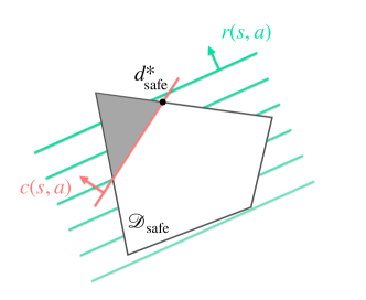
Figure 4: The dual linear program for a CMDP of two states and two actions.

Information Geometry of Policy Optimization

Among the most successful policy optimization schemes are natural policy gradient (NPG) methods or variants thereof like trust-region and proximal policy optimization (TRPO and PPO, respectively). These methods assume a convex geometry and corresponding Bregman divergences in the state-action polytope, where we refer to Neu et al. (2017); Müller & Montúfar (2023) for a more detailed discussion.

In general, a trust region update is defined as

$$\pi_{k+1}\in\operatorname*{arg\,max}_{\pi\in\Pi}\mathbb{A}_{r}^{\pi_{k}}(\pi)\quad\text{ sbj. to }D_{\Phi}(d_{\pi_{k}}||d_{\pi})\leq\delta,$$ (34)

where $D_{\Phi}\colon\mathscrsfs{D}\times\mathscrsfs{D}\to\mathbb{R}$ is a Bregman divergence induced by a suitably convex function $\Phi\colon\operatorname{int}(\mathscrsfs{D})\rightarrow\mathbb{R}$. The functional

$$\mathbb{A}_{r}^{\pi_{k}}(\pi)=\mathbb{E}_{s\sim d_{\pi_{k}},a\sim\pi_{\theta}(\cdot|s)}\big{[}A_{r}^{\pi_{k}}(s,a)\big{]},$$ (35)

as introduced in (Kakade & Langford, 2002), is called the policy advantage. As a loss function, it is also known as the surrogate advantage (Schulman et al., 2017a), since we can interpret $\mathbb{A}$ as a surrogate optimization objective of the return. In particular, it holds for a parameterized policy $\pi_{\theta}$, that $\nabla_{\theta}\mathbb{A}_{r}^{\pi_{\theta_{k}}}(\pi_{\theta})|_{\theta=\theta_{k}}=\nabla_{\theta}V_{r}(\theta_{k})$, see Kakade & Langford (2002); Schulman et al. (2017a). TRPO and the original NPG assume the same geometry (Kakade, 2001; Schulman et al., 2017a), since they employ an identical Bregman divergence

$$D_{\operatorname{K}}(d_{\pi_{1}}||d_{\pi_{2}}) \coloneqq\sum_{s,a}d_{\pi_{1}}(s,a)\log\frac{\pi_{1}(a|s)}{\pi_{2}(a|s)}=\sum_{s}d_{\pi_{1}}(s)D_{\operatorname{KL}}(\pi_{1}(\cdot|s)||\pi_{2}(\cdot|s)).$$

We refer to $D_{\operatorname{K}}$ as the Kakade divergence and informally write $D_{\operatorname{K}}(\pi_{1},\pi_{2})\coloneqq D_{\operatorname{K}}(d_{\pi_{1}},d_{\pi_{2}})$. This divergence can be shown to be the Bregman divergence induced by the negative conditional entropy

$$\Phi_{\operatorname{K}}(d_{\pi})\coloneqq\sum_{s,a}d_{\pi}(s,a)\log\pi(a|s),$$ (36)

see Neu et al. (2017). It is well known that with a parameterized policy $\pi_{\theta}$, a linear approximation of $\mathbb{A}$ and a quadratic approximation of the Bregman divergence $D_{\operatorname{K}}$ at $\theta$, one obtains the natural policy gradient step given by

$$\theta_{k+1}=\theta_{k}+\epsilon_{k}G_{\operatorname{K}}(\theta_{k})^{+}\nabla R(\theta_{k}),$$ (37)

where $G_{\operatorname{K}}(\theta)^{+}$ denotes a pseudo-inverse of the Gramian matrix with entries equal to the state-averaged Fisher-information matrix of the policy

$$G_{\operatorname{K}}(\theta)_{ij} \coloneqq\mathbb{E}_{s\sim d_{\pi_{\theta}}}\left[\sum_{a}\frac{\partial_{\theta_{i}}\pi_{\theta}(a|s)\partial_{\theta_{j}}\pi_{\theta}(a|s)}{\pi_{\theta}(a|s)}\right]$$ (38)

$$=\mathbb{E}_{d_{\pi_{\theta}}}[\partial_{\theta_{i}}\log\pi_{\theta}(a|s)\partial_{\theta_{j}}\log\pi_{\theta}(a|s)],$$ (39)

where we refer to Schulman et al. (2017a) and Section A.1 for a more detailed discussion.

A.1 Correspondence between TRPO and NPG

Consider a convex potential $\Phi\colon\mathscrsfs{D}\to\mathbb{R}$ or $\Phi\colon\mathscrsfs{D}_{\operatorname{safe}}\to\mathbb{R}$ and the TRPO update

$$\theta_{k+1}\in\operatorname*{arg\,max}L_{\theta_{k}}(\theta)\quad\text{sbj. to }D_{\Phi}(d_{\theta_{k}}||d_{\theta})\leq\epsilon,$$ (40)

where $L_{\theta}$… In practice, one uses a linear approximation of $L_{\theta_{k}}$ and a quadratic approximation of $D_{\Phi}$ to compute the TRPO update. This gives the following approximation of TRPO

$$\theta_{k+1}\in\operatorname*{arg\,max}\nabla_{\theta}\mathbb{A}_{r}^{\theta_{k}}(\theta)|_{\theta=\theta_{k}}\cdot\theta\quad\text{sbj. to }\lVert\theta_{k}-\theta\rVert_{G(\theta_{k})}^{2}\leq\epsilon,$$ (41)

where

$$G(\theta)_{ij}=\partial_{\theta_{i}}d_{\theta}^{\top}\nabla^{2}\Phi(d_{\theta})\partial_{\theta_{j}}d_{\theta}.$$ (42)

Note that by the policy gradient theorem, it holds that

$$\nabla_{\theta}\mathbb{A}_{r}^{\theta_{k}}(\theta)|_{\theta=\theta_{k}}=\nabla V_{r}(\theta_{k}).$$ (43)

Thus, the approximate TRPO update is equivalent to

$$\theta_{k+1}=\theta_{k}+\epsilon_{k}G(\theta_{k})^{+}\nabla V_{r}(\theta),$$ (44)

where

$$\epsilon_{k}=\frac{\sqrt{\epsilon}}{\lVert G(\theta_{k})^{+}\nabla V_{r}(\theta_{k})\rVert_{G(\theta_{k})}}.$$ (45)

Hence, the approximation TRPO update corresponds to a natural policy gradient update with an adaptively chosen step size.

Appendix B Details on the Safe Geometry for CMDPs

B.1 Safe Trust Regions

The safe mirror function for a single constraint is given by

$$\Phi_{\operatorname{C}}(d)\coloneqq\Phi_{\operatorname{K}}(d)+\sum_{i=1}^{m}\beta\,\phi(b-c^{\top}d),$$ (46)

and the resulting Bregman divergence

$$D_{{\operatorname{C}}}(d_{1}||d_{2})=\Phi_{\operatorname{C}}(d_{1})-\Phi_{\operatorname{C}}(d_{2})-\langle\nabla\Phi_{\operatorname{C}}(d_{2}),d_{1}-d_{2}\rangle.$$ (47)

is a linear operator in $\Phi$, hence

$$D_{\Phi(d)+\beta\phi(b-c^{\top}d)}(d_{1}||d_{2})=D_{\Phi_{\operatorname{K}}}(d_{1}||d_{2})+\beta D_{\phi}(d_{1}||d_{2}),$$ (48)

where

$$D_{\phi}(d_{1}||d_{2}) =\phi(b-c^{\top}d_{1})-\phi(b-c^{\top}d_{2})-\langle\nabla\phi(b-c^{\top}d_{2}),d_{1}-d_{2}\rangle$$ (49)

$$=\phi(b-c^{\top}d_{1})-\phi(b-c^{\top}d_{2})-\phi^{\prime}(b-c^{\top}d_{2})(c^{\top}d_{1}-c^{\top}d_{2}).$$ (50)

$$=\phi(b-V_{c}(\pi))-\phi(b-V_{c}(\pi_{k}))+\phi^{\prime}(b-V_{c}(\pi_{k}))(V_{c}(\pi)-V_{c}(\pi_{k})).$$ (51)

The last expression can be interpreted as the one-dimensional Bregman divergence $D_{\phi}(b-V_{c}(\pi)||b-V_{c}(\pi_{k}))$, which is a (strictly) convex function in $V_{c}(\pi)$ for fixed $\pi_{k}$ if $\phi$ is (strictly) convex.

B.2 Implementation Details

B.2.1 Surrogate Divergence

In Section A.1 we showed that TRPO with a quadratic approximation of the exact divergence $D_{\operatorname{C}}$ agrees with C-NPG with an adaptive stepsize choice. However, in practice, the exact constrained KL-Divergence $D_{\operatorname{C}}$ cannot be evaluated, because it depends on the cost-return of the optimized policy $V_{c}(\pi)$. Therefore, we use the surrogate divergence

$$\bar{D}_{\phi}(\pi_{\theta}||\pi_{\theta_{k}})=\phi(b-V_{c}^{\pi_{k}}-\mathbb{A}_{c}^{\pi_{k}}(\pi))-\phi(b-V_{c}^{\pi_{k}})+\phi^{\prime}(b-V_{c}^{\pi_{k}})\mathbb{A}_{c}^{\pi_{k}}(\pi)$$ (52)

is obtained by the substitution $V_{c}(\pi)-V_{c}^{\pi_{k}}\to\mathbb{A}_{c}^{\pi_{k}}(\pi)$ in $D_{\phi}$.

When we center this divergence around policy $\pi_{k}$ and keep this policy fixed, it becomes a function of the policy cost advantage.

$$\bar{D}_{\phi}(\pi_{\theta}||\pi_{\theta_{k}}) =\phi(b-V_{c}^{\pi_{k}}-\mathbb{A}_{c}^{\pi_{k}}(\pi))-\phi(b-V_{c}^{\pi_{k}})+\phi^{\prime}(b-V_{c}^{\pi_{k}})\mathbb{A}_{c}^{\pi_{k}}(\pi)$$

$$=\phi(\delta_{b}-\mathbb{A}_{c}^{\pi_{k}}(\pi))-\phi(\delta_{b})+\phi^{\prime}(\delta_{b})\mathbb{A}_{c}^{\pi_{k}}(\pi)$$

$$=\Psi(\mathbb{A}_{c}^{\pi_{k}}).$$

Note that $\bar{D}_{\phi}(\pi_{\theta}||\pi_{\theta_{k}})=\Psi(\mathbb{A}_{c}^{\pi_{k}}(\pi))$, where $\Psi(x)=\phi(\delta_{b}-x)-\phi(\delta_{b})-\phi^{\prime}(\delta_{b})\cdot x$ is a (strictly) convex function if $\phi$ is (strictly) convex, since it is equivalent to the one-dimensional Bregman divergence $D_{\phi}(\delta_{b}-x||\delta_{b})$ on the domain of $\phi(b-x)$, see Figure 5.

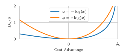
Figure 5: The surrogate Constrained KL-Divergence as a function of the policy cost advantage.

Example 8.

The function $\phi(x)=x\log(x)$ induces the divergence

$$\bar{D}_{\phi}(\pi_{\theta}||\pi_{\theta_{k}})=\mathbb{A}_{c}^{\pi_{k}}(\pi_{\theta})-(\delta_{b}-\mathbb{A}_{c}^{\pi_{k}}(\pi_{\theta}))\log\left(\frac{\delta_{b}}{\delta_{b}-\mathbb{A}_{c}^{\pi_{k}}(\pi_{\theta}))}\right).\\$$ (53)

B.2.2 Quadratic Approximation

In the proof that TRPO with quadratic approximation agrees with a natural gradient step we have used that $\nabla_{\theta}\mathbb{A}_{r}^{\theta_{k}}(\theta)|_{\theta=\theta_{k}}=\nabla V_{r}(\theta_{k})$, which holds although $\mathbb{A}_{r}$ is only a proxy of $V_{r}$. We now provide a similar property for the quadratic approximation of the surrogate divergences $\bar{D}_{\phi}$ and $\bar{D}_{\operatorname{KL}}$.

Proposition 9.

For any parameter $\theta$ with $\pi_{\theta}\in\Pi_{\operatorname{safe}}$ it holds that

$$\nabla_{\theta}^{2}\bar{D}_{\phi}(\theta||\hat{\theta})|_{\theta=\hat{\theta}}=\nabla_{\theta}^{2}{D}_{\phi}(\theta||\hat{\theta})|_{\theta=\hat{\theta}}$$ (54)

and hence

$$\nabla_{\theta}^{2}\bar{D}_{\textup{KL}}(\theta||\hat{\theta})|_{\theta=\hat{\theta}}+\beta\nabla_{\theta}^{2}\bar{D}_{\phi}(\theta||\hat{\theta})|_{\theta=\hat{\theta}}=G_{\operatorname{C}}(\hat{\theta})$$ (55)

where $G_{\operatorname{C}}(\theta)$ denotes the Gramian matrix of C-NPG with entries

$$G_{\operatorname{C}}({\theta})_{ij}=\partial_{\theta_{i}}d_{\theta}^{\top}\nabla^{2}\Phi_{\operatorname{C}}(\theta)\partial_{\theta_{j}}d_{\theta}.$$ (56)

Proof.

Let $\bar{H}_{\operatorname{KL}}(\theta)=\nabla^{2}_{\theta}\bar{D}_{\operatorname{KL}}(\theta||\hat{\theta})|_{\theta=\hat{\theta}}$ and $\bar{H}_{\phi}(\theta)=\nabla^{2}_{\theta}\bar{D}_{\phi}(\theta||\hat{\theta})|_{\theta=\hat{\theta}}$. One can show that $\bar{H}_{\textup{KL}}=G_{\operatorname{K}}(\theta)$ (Schulman et al., 2017a). Further, we have

$$\bar{H}_{\phi}(\theta) =\mathbf{J}_{\theta}\mathbb{A}_{c}^{\pi_{k}}(\theta)^{\top}\nabla^{2}\Psi(\mathbb{A}_{c}^{\pi_{k}}(\theta))\mathbf{J}_{\theta}\mathbb{A}_{c}^{\pi_{k}}(\theta)+\mathbf{J}\Psi(\mathbb{A}_{c}^{\pi_{k}}(\theta))^{\top}\nabla^{2}_{\theta}\mathbb{A}_{c}^{\pi_{k}}(\theta)$$

$$\overset{a)}{=}\mathbf{J}_{\theta}\mathbb{A}_{c}^{\pi_{k}}(\theta)^{\top}\nabla^{2}\Psi(\mathbb{A}_{c}^{\pi_{k}}(\theta))\mathbf{J}_{\theta}\mathbb{A}_{c}^{\pi_{k}}(\theta)$$

$$\overset{b)}{=}\mathbf{J}_{\theta}\mathbb{A}_{c}^{\pi_{k}}(\theta)^{\top}\phi^{\prime\prime}(b-V_{c}^{\pi_{k}}(\theta))\mathbf{J}_{\theta}\mathbb{A}_{c}^{\pi_{k}}(\theta)$$

$$=\mathbf{J}_{\theta}V_{c}^{\pi_{k}}(\theta)^{\top}\phi^{\prime\prime}(b-V_{c}^{\pi_{k}}(\theta))\mathbf{J}_{\theta}V_{c}^{\pi_{k}}(\theta),$$

where a) follows from $\mathbf{J}\Psi(\mathbb{A}_{c}^{\pi_{k}}(\theta))=0$ since $\Psi(0)=0$, $\Psi\geq 0$ and $\mathbb{A}_{c}^{\hat{\theta}}(\theta)|_{\theta=\hat{\theta}}=0$. Further, b) follows because $\nabla^{2}\Psi(x)|_{x=0}=\phi^{\prime\prime}(\delta_{b})$. Thus, $\nabla^{2}_{\theta}\bar{D}_{\operatorname{C}}$ is equivalent to C-TRPO’s Gramian

$$G_{\operatorname{C}}(\theta)_{ij} \coloneqq G_{\operatorname{K}}(\theta)_{ij}+\beta\phi^{\prime\prime}(b-c_{k}^{\top}d_{\theta})\partial_{\theta_{i}}d_{\theta}^{\top}cc^{\top}\partial_{\theta_{i}}d_{\theta}$$ (57)

$$=\bar{H}_{\operatorname{KL}}+\sum_{l}\beta_{l}\mathbf{J}_{\theta}V_{c}(\theta)^{\top}\phi^{\prime\prime}(b-V_{c}(\theta))\mathbf{J}_{\theta}V_{c}(\theta),$$ (58)

$$=\bar{H}_{\operatorname{KL}}+\beta\bar{H}_{\phi}.$$ (59)

Again, for multiple constraints, the statement follows analogously. ∎

In particular, this shows that the C-TRPO update can be interpreted as a natural policy gradient step with an adaptive step size and that the updates with $D_{\operatorname{C}}$ and $\bar{D}_{\operatorname{C}}$ are equivalent if we use a quadratic approximation for both, justifying $\bar{D}_{\operatorname{C}}$ as a surrogate for $D_{\operatorname{C}}$.

In the approximate case of C-TRPO and CPO, where the reward is approximated linearly, and the trust region quadratically, the constraints differ in that C-TRPO’s constraint is

$$(\theta-\theta_{k})(\bar{H}_{\operatorname{KL}}(\theta)+\beta\bar{H}_{\phi}(\theta))(\theta-\theta_{k})<\delta$$

whereas CPO’s is

$$(\theta-\theta_{k})\bar{H}_{\operatorname{KL}}(\theta)(\theta-\theta_{k})<\delta\text{ and }V_{c}^{\theta_{k}}+(\nabla_{\theta}\mathbb{A}^{\theta_{k}}_{c}(\theta))^{\top}(\theta-\theta_{k})\leq b.$$

B.2.3 Estimation of the divergence

In the practical implementation, the expected KL-divergence between the policy of the previous iteration, $\pi_{k}$, and the proposal policy $\pi$ is estimated from state samples $s_{i}$ by running $\pi_{k}$ in the environment

$$\sum_{s}d_{\pi_{k}}(s)D_{\operatorname{KL}}(\pi(\cdot|s)||\pi_{k}(\cdot|s))\approx 1/N\sum_{i=0}^{N-1}D_{\operatorname{KL}}({\pi}(\cdot|s_{i})||{\pi_{k}}(\cdot|s_{i}))$$ (60)

where $D_{\operatorname{KL}}$ can be computed in closed form for Gaussian policies, where $N$ is the batch size.

For the constraint term, we estimate $\delta_{b}$ from trajectory samples, as well as the policy cost advantage

$$\mathbb{A}_{c}^{\pi_{k}}(\pi)\approx\mathbb{\hat{A}}=\frac{1}{N}\sum_{i=0}^{N-1}\frac{\pi(a_{i}|s_{i})}{\pi_{k}(a_{i}|s_{i})}\hat{A}^{\pi_{k}}_{i}$$ (61)

where $\hat{A}^{\pi_{k}}_{i}$ is the GAE-$\lambda$ estimate of the advantage function (Schulman et al., 2018). For any suitable $\phi$, the resulting divergence estimate is

$$\hat{D}_{\phi} =\phi(\delta_{b}-\mathbb{\hat{A}})-\phi(\delta_{b})-\phi^{\prime}(\delta_{b})\mathbb{\hat{A}}$$ (62)

and for the specific choice $\phi(x)=x\log(x)$

$$\hat{D}_{\phi}=\mathbb{\hat{A}}-(\delta_{b}-\mathbb{\hat{A}})\log\left(\frac{\delta_{b}}{\delta_{b}-\mathbb{\hat{A}}}\right).$$ (63)

B.2.4 Connection to performance improvement bounds

In a series of works (Kakade & Langford, 2002; Pirotta et al., 2013; Schulman et al., 2017a; Achiam et al., 2017), the following bound on policy performance difference between two policies has been established.

$$V_{f}(\pi^{\prime})-V_{f}(\pi)\lesseqgtr\mathbb{A}^{\pi^{\prime}}_{f}(\pi)\pm\frac{2\gamma\epsilon_{f}}{(1-\gamma)}\mathbb{E}_{s\sim d_{\pi}}D_{\operatorname{TV}}(\pi^{\prime}||\pi)(s)$$ (64)

where $D_{\operatorname{TV}}$ is the Total Variation Distance. Furthermore, by Pinsker’s inequality, we have that

$$D_{\operatorname{TV}}(\pi^{\prime}||\pi)\leq\sqrt{\frac{1}{2}D_{\operatorname{KL}}(\pi^{\prime}||\pi)},$$ (65)

and by Jensen’s inequality

$$\mathbb{E}_{s\sim d_{\pi}}D_{\operatorname{TV}}(\pi^{\prime}||\pi)(s)\leq\sqrt{\frac{1}{2}\mathbb{E}_{s\sim d_{\pi}}D_{\operatorname{KL}}(\pi^{\prime}||\pi)(s)},$$ (66)

It follows that we can not only substitute the KL-divergence into the bound but any divergence

$$D_{\Phi}(d_{\pi}^{\prime}||d_{\pi})\geq\mathbb{E}_{s\sim d_{\pi}}D_{\operatorname{KL}}(\pi^{\prime}||\pi)(s)$$ (67)

can be substituted, and still retains TRPO’s and CPO’s update guarantees.

Appendix C Proofs of Section 4

C.1 Proofs of Section 4.1

See 2

Proof.

It follows from the lower bound in Theorem 1 that

$$V_{r}(\pi_{k+1})-V_{r}(\pi_{k})\geq\mathbb{A}^{\pi_{k}}_{r}(\pi_{k+1})-\frac{\gamma\epsilon_{r}}{(1-\gamma)}\sqrt{2\bar{D}_{\operatorname{C}}(\pi_{k+1}||\pi_{k})}$$ (68)

where we choose $f=r$. The bound holds because $\bar{D}_{\phi}\geq 0$, and thus $\bar{D}_{\operatorname{C}}\geq\mathbb{E}D_{\operatorname{KL}}$. Further, $\delta\geq D_{\operatorname{C}}$ and $\mathbb{A}^{\pi_{k}}_{r}(\pi_{k+1})\geq 0$ by the update equation, which concludes the proof. See Appendix B.2.4 for a more detailed discussion. ∎

See 3

Proof.

Let us fix a strictly safe policy $\pi_{0}\in\operatorname{int}(\Pi_{\textup{safe}})$. In both cases, we approximate the expected cost of a policy using $V_{c}(\pi)\approx V_{c}(\pi_{0})+\mathbb{A}_{c}^{\pi_{0}}(\pi)$, which is off by the advantage mismatch term in Proposition 2. Hence, we maximize the surrogate of the expected value $\mathbb{A}^{\pi_{0}}_{r}(\pi)$ over the regions

$$P_{\textup{CPO}}\coloneqq\{\pi\in\Pi:\bar{D}_{\operatorname{K}}(\pi,\pi_{0})\leq\delta,\,V_{c}(\pi_{0})+\mathbb{A}_{c}^{\pi_{0}}(\pi)\leq b\}$$

in the case of CPO, and

$$P_{\beta}\coloneqq\{\pi\in\Pi:\bar{D}_{\operatorname{C}}(\pi,\pi_{0})\leq\delta\},$$

with C-TRPO for some $\beta>0$. Note that

$$\bar{D}_{\operatorname{C}}(\pi,\pi_{0})=\bar{D}_{\operatorname{K}}(\pi,\pi_{0})+\beta\Psi(\mathbb{A}_{c}^{\pi_{0}}(\pi)),$$ (69)

and $\Psi\colon(-\infty,\delta_{b})\to(0,+\infty)$ and $\Psi(t)\to+\infty$ for $t\nearrow\delta_{b}$, where $\delta_{b}=b-V_{c}(\pi_{0})$. Denote the corresponding updates by $\hat{\pi}_{\textup{CPO}}$ and the C-TRPO update by $\hat{\pi}_{\beta}$. Note that we have $P_{\beta}\subseteq P_{\beta^{\prime}}\subseteq P_{\operatorname{CPO}}$ for $\beta\geq\beta^{\prime}$. Further, we have

$$\bigcup_{\beta>0}P_{\beta}=\{\pi\in P:D_{\operatorname{K}}(\pi,\pi_{0})<\delta,V_{c}(\pi_{0})+\mathbb{A}_{c}^{\pi_{0}}(\pi)<b\}.$$

Hence, the trust regions $P_{\beta}$ grow for $\beta\searrow 0$ and fill the interior of the trust region $P_{\textup{CPO}}$. ∎

Remark 10.

Intuitively, one could repeatedly solve the C-TRPO problem with successively smaller values of $\beta$, which would be similar to solving CPO with the interior point method using $\phi$ as the barrier function.

See 4

Proof.

Setting $f=c$ in the upper bound from Theorem 1, and replacing $\mathbb{E}D_{\mathrm{KL}}$ with $\delta$ as in Proposition 2 results in

$$V_{c}(\pi_{k+1})\leq V_{c}(\pi_{k})+\mathbb{A}_{c}^{\pi_{k}}(\pi_{k+1})+\frac{\sqrt{2\delta}\gamma\epsilon_{c}}{1-\gamma}.$$ (70)

Recall that $\bar{D}_{\operatorname{C}}=\bar{D}_{\operatorname{K}}+\beta\bar{D}_{\phi}$ and that $\bar{D}_{\phi}(\pi_{k+1}||\pi_{k})=\Psi(\mathbb{A}_{c}^{\pi_{k}}(\pi_{k+1}))$, where $\Psi(x)=\phi(\delta_{b}-x)-\phi(\delta_{b})-\phi^{\prime}(\delta_{b})\cdot x$. By the definition of the update it holds that

$$\Psi(\mathbb{A}_{c}^{\pi_{k}}(\pi_{k+1}))<\delta/\beta.$$ (71)

Since we are only interested in upper bounding the worst case, we can focus on $\mathbb{A}_{c}^{\pi_{k}}(\pi_{k+1})>0$, so we restrict $\Psi\colon[0,\delta_{b})\to[0,\infty)$. Further, for strictly convex $\phi$, $\Psi$ is strictly convex and increasing with increasing inverse. It follows that

$$\mathbb{A}_{c}^{\pi_{k}}(\pi_{k+1})<\Psi^{-1}(\delta/\beta),$$ (72)

with $\Psi^{-1}\colon[0,\infty)\to[0,\delta_{b})$, which concludes the proof. ∎

C.2 Proofs of Section 4.2

Recall that we study the natural policy gradient flow

$$\partial_{t}\theta_{t}=G_{\operatorname{C}}(\theta_{t})^{+}\nabla V_{r}(\theta_{t}),$$ (73)

where $G_{\operatorname{C}}(\theta)^{+}$ denotes a pseudo-inverse of $G_{\operatorname{C}}(\theta)$ with entries

$$\begin{split}G_{\operatorname{C}}(\theta)_{ij}&\coloneqq\partial_{\theta_{i}}d_{\theta}^{\top}\nabla^{2}\Phi_{\operatorname{C}}(d_{\theta})\partial_{\theta_{j}}d_{\theta}=G_{\operatorname{K}}(\theta)_{ij}+\sum_{k}\beta_{k}\phi^{\prime\prime}(b_{k}-c_{k}^{\top}d_{\theta})\partial_{\theta_{i}}d_{\theta}^{\top}c_{k}c_{k}^{\top}\partial_{\theta_{i}}d_{\theta}.\end{split}$$ (74)

and $\theta\mapsto\pi_{\theta}$ is a differentiable policy parametrization.

Moreover, we assume that $\theta\mapsto\pi_{\theta}$ is regular, that it is surjective and the Jacobian is of maximal rank everywhere. This assumption implies overparametrization but is satisfied for common models like tabular softmax, tabular escort, or expressive log-linear policy parameterizations (Agarwal et al., 2021a; Mei et al., 2020a; Müller & Montúfar, 2023).

We denote the set of safe parameters by $\Theta_{\operatorname{safe}}\coloneqq\{\theta\in\mathbb{R}^{p}:\pi_{\theta}\in\Pi_{\operatorname{safe}}\}$, which is non-convex in general and say that $\Theta_{\operatorname{safe}}$ is invariant under Equation 23 if $\theta_{0}\in\Theta_{\operatorname{safe}}$ implies $\theta_{t}\in\Theta_{\operatorname{safe}}$ for all $t$. Invariance is associated with safe control during optimization and is typically achieved via control barrier function methods (Ames et al., 2017; Cheng et al., 2019). We study the evolution of the state-action distributions $d_{t}=d^{\pi_{\theta_{t}}}$ as this allows us to employ the linear programming formulation of CMPDs and we obtain the following convergence guarantees.

See 5

Proof.

Consider a solution $(\theta_{t})_{t>0}$ of Equation 73. As the mapping $\pi\mapsto d^{\pi}$ is a diffeomorphism (Müller & Montúfar, 2023) the parameterization $\Theta_{\operatorname{safe}}\to\mathscrsfs{D}_{\operatorname{safe}},\theta\mapsto d^{\pi_{\theta}}$ is surjective and has a Jacobian of maximal rank everywhere. As $G_{\operatorname{C}}(\theta)_{ij}=\partial_{\theta_{i}}d_{\theta}\nabla\Phi_{\operatorname{C}}\partial_{\theta_{i}}d_{\theta}$ this implies that the state-action distributions $d_{t}=d^{\pi_{\theta_{t}}}$ solve the Hessian gradient flow with Legendre-type function $\Phi_{\operatorname{C}}$ and the linear objective $d\mapsto r^{\top}d$, see Amari (2016); van Oostrum et al. (2023); Müller & Montúfar (2023) for a more detailed discussion. It suffices to study the gradient flow in the space of state-action distributions $d_{t}$. It is easily checked that $\Phi_{\operatorname{C}}$ is a Legendre-type function for the convex domain $\mathscrsfs{D}_{{\operatorname{C}}}$, meaning that it satisfies $\lVert\nabla\Phi(d_{n})\rVert\to+\infty$ for $d_{n}\to d\in\partial\mathscrsfs{D}_{\operatorname{safe}}$. Since the objective is linear, it follows from the general theory of Hessian gradient flows of convex programs that the flow is well posed, see Alvarez et al. (2004); Müller & Montúfar (2023). ∎

See 6

Proof.

Just like in the proof of Theorem 6 we see that $d_{t}=d^{\pi_{\theta_{t}}}$ solves the Hessian gradient flow with respect to the Legendre type function $\Phi_{\operatorname{C}}$. Now the claims regarding convergence and the identification of the limit $\lim_{t\to+\infty}\pi_{\theta_{t}}$ follows from the general theory of Hessian gradient flows, see Alvarez et al. (2004); Müller et al. (2024). ∎

Appendix D Additional Experiments

To better understand the effects of the two hyperparameters $\beta$ and $b_{\textsc{H}}$, we observe how they change the training dynamics through the example of the AntVelocity environment. Further, we visualize learning curves for all environments compared to CPO and PCPO as representative baselines.

D.1 Effects of the hyper-parameters

The safety parameter $\beta$ modulates the stringency with which C-TRPO satisfies the constraint, without limiting the expected return for values up to $\beta=1$, see Figure 6. For higher values, the expected return starts to degrade, partly due to $\bar{D}_{\phi}$ being relatively noisy compared to $\bar{D}_{\operatorname{KL}}$ and thus we recommend the choice $\beta=1$.

Further, we observe that constraint satisfaction is stable across different choices of cost threshold $b$, see Figure 7, and that in most environments, constraint violations seem to reduce as the algorithm converges, meaning that the regret flattens over time. This behavior suggests that the divergence estimation becomes increasingly accurate over time, potentially allowing C-TRPO to achieve sublinear regret. However, we leave regret analysis of the finite sample regime for future research.

Finally, employing a hysteresis fraction $0<b_{\textsc{H}}<b$ seems beneficial, possible because it leads the iterate away from the boundary of the safe set, and because divergence estimates tend to be more reliable for strictly safe policies. The effect of the choice of $b_{\textsc{H}}$ is visualized in Figure 8.

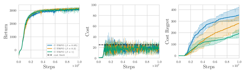
Figure 6: Changing $\beta$ influences the degree of safety.

Figure 7: The constraint satisfaction is robust to changing the cost limit.

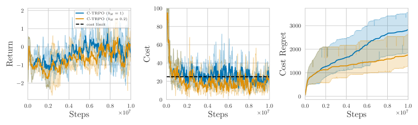
Figure 8: In difficult environments, e.g. those that start off in the unsafe policy set, it seems to be beneficial to set a fraction of the cost limit for hysteresis.

D.2 Performance on individual environments

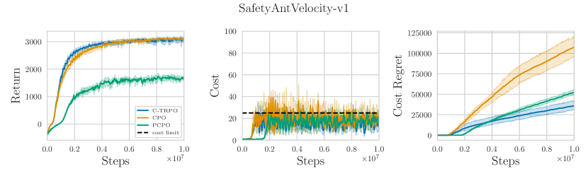
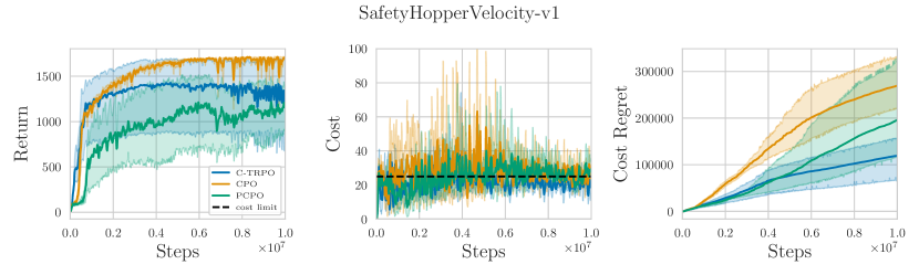
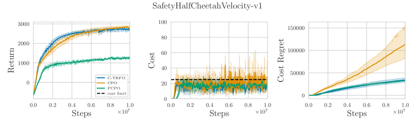
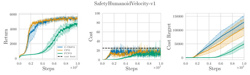
Figure 9: C-TRPO vs. CPO and PCPO in the locomotion environments.

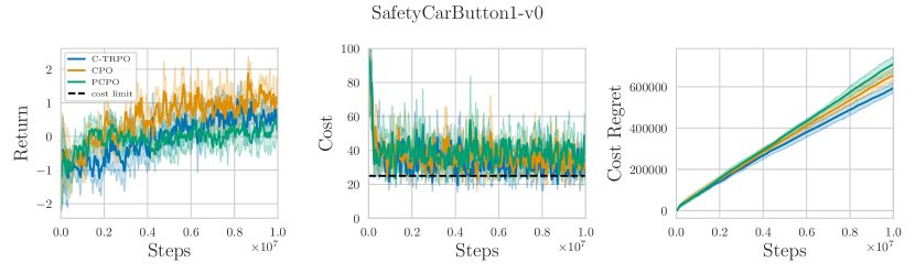
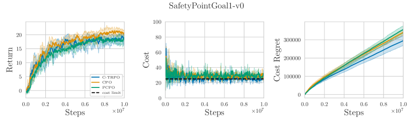
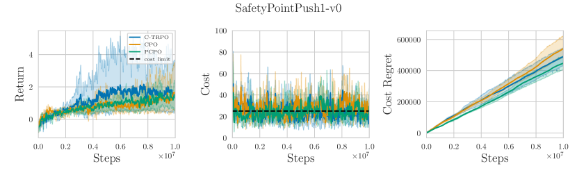
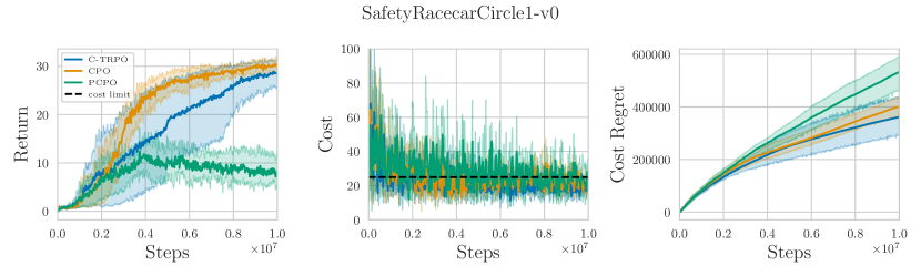
Figure 10: C-TRPO vs. CPO and PCPO in the navigation environments.

Table 1: Average evaluation performance per task across 10 evaluation runs and 5 seeds each.

	PCPO		PPO		CPPO-PID		CPO		C-TRPO		TRPO-Lag		PPO-Lag
	$V_{r}$	$V_{c}$	$V_{r}$	$V_{c}$	$V_{r}$	$V_{c}$	$V_{r}$	$V_{c}$	$V_{r}$	$V_{c}$	$V_{r}$	$V_{c}$	$V_{r}$	$V_{c}$
AntVelocity	2045.9	54.2	1828.2	19.5	1810.0	18.8	2537.7	5.2	2736.1	6.1	2893.0	14.4	1763.7	18.3
HalfCheetahVelocity	1391.7	65.5	4023.2	831.8	2329.1	6.7	1988.5	20.4	2224.0	8.4	2448.0	14.7	2359.9	3.9
HumanoidVelocity	561.7	0.0	4384.8	5.5	4638.3	5.1	5653.4	0.0	4950.0	5.9	5603.0	0.0	4212.8	7.9
HopperVelocity	799.5	12.3	902.0	224.7	1490.6	2.7	1420.4	0.6	1333.6	7.7	487.1	19.1	101.2	4.5
CarButton1	-1.5	76.7	17.9	374.3	-1.1	40.7	-1.0	72.7	-5.0	41.2	-7.2	28.6	2.9	127.0
PointGoal1	11.9	22.4	26.4	50.3	1.4	17.8	13.3	16.2	13.8	24.4	25.0	37.5	18.4	48.1
RacecarCircle1	4.7	23.4	39.5	191.1	0.9	13.4	7.5	16.2	8.8	39.5	23.3	3.9	10.1	2.6
PointPush1	1.1	27.8	1.1	37.1	0.5	25.3	0.6	52.8	0.8	17.5	0.5	21.1	0.5	37.8

References

- Achiam et al. (2017) Joshua Achiam, David Held, Aviv Tamar, and Pieter Abbeel. Constrained policy optimization, 2017.
- Agarwal et al. (2021a) Alekh Agarwal, Sham M Kakade, Jason D Lee, and Gaurav Mahajan. On the theory of policy gradient methods: Optimality, approximation, and distribution shift. The Journal of Machine Learning Research, 22(1):4431–4506, 2021a.
- Agarwal et al. (2021b) Rishabh Agarwal, Max Schwarzer, Pablo Samuel Castro, Aaron C Courville, and Marc Bellemare. Deep reinforcement learning at the edge of the statistical precipice. Advances in Neural Information Processing Systems, 34, 2021b.
- Altman (1999) Eitan Altman. Constrained Markov Decision Processes. CRC Press, Taylor & Francis Group, 1999. URL https://api.semanticscholar.org/CorpusID:14906227.
- Alvarez et al. (2004) Felipe Alvarez, Jérôme Bolte, and Olivier Brahic. Hessian riemannian gradient flows in convex programming. SIAM journal on control and optimization, 43(2):477–501, 2004.
- Amari (2016) Shun-ichi Amari. Information geometry and its applications, volume 194. Springer, 2016.
- Ames et al. (2017) Aaron D. Ames, Xiangru Xu, Jessy W. Grizzle, and Paulo Tabuada. Control barrier function based quadratic programs for safety critical systems. IEEE Transactions on Automatic Control, 62(8):3861–3876, August 2017. ISSN 1558-2523. doi: 10.1109/tac.2016.2638961. URL http://dx.doi.org/10.1109/TAC.2016.2638961.
- Berkenkamp et al. (2017) Felix Berkenkamp, Matteo Turchetta, Angela Schoellig, and Andreas Krause. Safe model-based reinforcement learning with stability guarantees. In I. Guyon, U. Von Luxburg, S. Bengio, H. Wallach, R. Fergus, S. Vishwanathan, and R. Garnett (eds.), Advances in Neural Information Processing Systems, volume 30. Curran Associates, Inc., 2017. URL https://proceedings.neurips.cc/paper_files/paper/2017/file/766ebcd59621e305170616ba3d3dac32-Paper.pdf.
- Cheng et al. (2019) Richard Cheng, Gabor Orosz, Richard M. Murray, and Joel W. Burdick. End-to-end safe reinforcement learning through barrier functions for safety-critical continuous control tasks, 2019. URL https://arxiv.org/abs/1903.08792.
- Chow et al. (2019) Yinlam Chow, Ofir Nachum, Aleksandra Faust, Edgar Duenez-Guzman, and Mohammad Ghavamzadeh. Lyapunov-based safe policy optimization for continuous control, 2019. URL https://arxiv.org/abs/1901.10031.
- Dey et al. (2024) Sumanta Dey, Pallab Dasgupta, and Soumyajit Dey. P2bpo: Permeable penalty barrier-based policy optimization for safe rl. In Proceedings of the AAAI Conference on Artificial Intelligence, volume 38, pp. 21029–21036, 2024.
- Efroni et al. (2020) Yonathan Efroni, Shie Mannor, and Matteo Pirotta. Exploration-exploitation in constrained mdps, 2020. URL https://arxiv.org/abs/2003.02189.
- Feinberg & Shwartz (2012) Eugene A Feinberg and Adam Shwartz. Handbook of Markov decision processes: methods and applications, volume 40. Springer Science & Business Media, 2012.
- Ji et al. (2023) Jiaming Ji, Borong Zhang, Jiayi Zhou, Xuehai Pan, Weidong Huang, Ruiyang Sun, Yiran Geng, Yifan Zhong, Juntao Dai, and Yaodong Yang. Safety-gymnasium: A unified safe reinforcement learning benchmark, 2023.
- Kakade & Langford (2002) Sham Kakade and John Langford. Approximately optimal approximate reinforcement learning. In Proceedings of the Nineteenth International Conference on Machine Learning, ICML ’02, pp. 267–274, San Francisco, CA, USA, 2002. Morgan Kaufmann Publishers Inc. ISBN 1558608737.
- Kakade (2001) Sham M Kakade. A natural policy gradient. Advances in neural information processing systems, 14, 2001.
- Kallenberg (1994) Lodewijk CM Kallenberg. Survey of linear programming for standard and nonstandard markovian control problems. part i: Theory. Zeitschrift für Operations Research, 40:1–42, 1994.
- Konda & Tsitsiklis (1999) Vijay Konda and John Tsitsiklis. Actor-critic algorithms. In S. Solla, T. Leen, and K. Müller (eds.), Advances in Neural Information Processing Systems, volume 12. MIT Press, 1999. URL https://proceedings.neurips.cc/paper_files/paper/1999/file/6449f44a102fde848669bdd9eb6b76fa-Paper.pdf.
- Liu et al. (2021) Zhuang Liu, Xuanlin Li, Bingyi Kang, and Trevor Darrell. Regularization matters in policy optimization - an empirical study on continuous control. In International Conference on Learning Representations, 2021. URL https://openreview.net/forum?id=yr1mzrH3IC.
- Mei et al. (2020a) Jincheng Mei, Chenjun Xiao, Bo Dai, Lihong Li, Csaba Szepesvári, and Dale Schuurmans. Escaping the gravitational pull of softmax. Advances in Neural Information Processing Systems, 33:21130–21140, 2020a.
- Mei et al. (2020b) Jincheng Mei, Chenjun Xiao, Csaba Szepesvari, and Dale Schuurmans. On the global convergence rates of softmax policy gradient methods. In International Conference on Machine Learning, pp. 6820–6829. PMLR, 2020b.
- Müller & Montúfar (2023) Johannes Müller and Guido Montúfar. Geometry and convergence of natural policy gradient methods. Information Geometry, pp. 1–39, 2023.
- Müller et al. (2024) Johannes Müller, Semih Çaycı, and Guido Montúfar. Fisher-rao gradient flows of linear programs and state-action natural policy gradients. arXiv preprint arXiv:2403.19448, 2024.
- Müller et al. (2024) Adrian Müller, Pragnya Alatur, Volkan Cevher, Giorgia Ramponi, and Niao He. Truly no-regret learning in constrained mdps, 2024. URL https://arxiv.org/abs/2402.15776.
- Neu et al. (2017) Gergely Neu, Anders Jonsson, and Vicenç Gómez. A unified view of entropy-regularized markov decision processes. arXiv preprint arXiv:1705.07798, 2017.
- Ni & Kamgarpour (2024) Tingting Ni and Maryam Kamgarpour. A safe exploration approach to constrained markov decision processes. In ICML 2024 Workshop: Foundations of Reinforcement Learning and Control–Connections and Perspectives, 2024.
- Pirotta et al. (2013) Matteo Pirotta, Marcello Restelli, Alessio Pecorino, and Daniele Calandriello. Safe policy iteration. In Sanjoy Dasgupta and David McAllester (eds.), Proceedings of the 30th International Conference on Machine Learning, volume 28 of Proceedings of Machine Learning Research, pp. 307–315, Atlanta, Georgia, USA, 17–19 Jun 2013. PMLR. URL https://proceedings.mlr.press/v28/pirotta13.html.
- Ray et al. (2019) Alex Ray, Joshua Achiam, and Dario Amodei. Benchmarking safe exploration in deep reinforcement learning. arXiv preprint arXiv:1910.01708, 7(1):2, 2019.
- Schulman et al. (2017a) John Schulman, Sergey Levine, Philipp Moritz, Michael I. Jordan, and Pieter Abbeel. Trust region policy optimization, 2017a.
- Schulman et al. (2017b) John Schulman, Filip Wolski, Prafulla Dhariwal, Alec Radford, and Oleg Klimov. Proximal policy optimization algorithms, 2017b. URL https://arxiv.org/abs/1707.06347.
- Schulman et al. (2018) John Schulman, Philipp Moritz, Sergey Levine, Michael Jordan, and Pieter Abbeel. High-dimensional continuous control using generalized advantage estimation, 2018. URL https://arxiv.org/abs/1506.02438.
- Sohrabi et al. (2024) Motahareh Sohrabi, Juan Ramirez, Tianyue H. Zhang, Simon Lacoste-Julien, and Jose Gallego-Posada. On pi controllers for updating lagrange multipliers in constrained optimization, 2024. URL https://arxiv.org/abs/2406.04558.
- Stooke et al. (2020) Adam Stooke, Joshua Achiam, and Pieter Abbeel. Responsive safety in reinforcement learning by pid lagrangian methods, 2020. URL https://arxiv.org/abs/2007.03964.
- Sutton et al. (1999) Richard S Sutton, David McAllester, Satinder Singh, and Yishay Mansour. Policy gradient methods for reinforcement learning with function approximation. In S. Solla, T. Leen, and K. Müller (eds.), Advances in Neural Information Processing Systems, volume 12. MIT Press, 1999. URL https://proceedings.neurips.cc/paper_files/paper/1999/file/464d828b85b0bed98e80ade0a5c43b0f-Paper.pdf.
- Tomar et al. (2022) Manan Tomar, Lior Shani, Yonathan Efroni, and Mohammad Ghavamzadeh. Mirror descent policy optimization. In International Conference on Learning Representations, 2022. URL https://openreview.net/forum?id=aBO5SvgSt1.
- Usmanova et al. (2024) Ilnura Usmanova, Yarden As, Maryam Kamgarpour, and Andreas Krause. Log barriers for safe black-box optimization with application to safe reinforcement learning. Journal of Machine Learning Research, 25(171):1–54, 2024.
- van Oostrum et al. (2023) Jesse van Oostrum, Johannes Müller, and Nihat Ay. Invariance properties of the natural gradient in overparametrised systems. Information geometry, 6(1):51–67, 2023.
- Williams (1992) Ronald J Williams. Simple statistical gradient-following algorithms for connectionist reinforcement learning. Machine learning, 8:229–256, 1992.
- Yang et al. (2020) Tsung-Yen Yang, Justinian Rosca, Karthik Narasimhan, and Peter J. Ramadge. Projection-based constrained policy optimization, 2020. URL https://arxiv.org/abs/2010.03152.
- Zhang et al. (2024) Baohe Zhang, Yuan Zhang, Lilli Frison, Thomas Brox, and Joschka Bödecker. Constrained reinforcement learning with smoothed log barrier function. arXiv preprint arXiv:2403.14508, 2024.
- Zhang et al. (2022) Linrui Zhang, Li Shen, Long Yang, Shixiang Chen, Bo Yuan, Xueqian Wang, and Dacheng Tao. Penalized proximal policy optimization for safe reinforcement learning, 2022. URL https://arxiv.org/abs/2205.11814.