Rational Extension of Anisotropic Harmonic Oscillator Potentials in Higher Dimensions

Abstract

This paper presents the first-order supersymmetric rational extension of the quantum anisotropic harmonic oscillator (QAHO) in multiple dimensions, including full-line, half-line, and their combinations. The exact solutions are in terms of the exceptional orthogonal polynomials. The rationally extended potentials are isospectral to the conventional QAHOs.

1 Introduction

Supersymmetric Quantum Mechanics (SUSY QM) [1, 2, 3, 4, 5, 6, 7] is a powerful factorization method that has proven useful for generating new system of potentials from the known ones. In recent years, after the discovery of the exceptional orthogonal polynomials (EOPs) [8, 9], a family of new potentials, isospectral to the corresponding conventional potentials were discovered [10, 11, 12, 13, 14, 15, 16, 17, 18]. Apart from the other applications, rational extension of the isotropic harmonic oscillator was also done [18]. The extended eigenfunctions were expressed in terms of the exceptional Laguerre polynomials. Following this SUSY approach, a family of one-dimensional anharmonic oscillator potentials [19] which are strictly isospectral to the harmonic oscillator potential defined on the full-line have also been constructed for even co-dimension $m$. Solutions of these potentials are obtained in terms of exceptional Hermite polynomials. In this case, it has been shown that the SUSY partner potential can have factorization energy above the ground state energy of the conventional potential. Building on this foundation and following the same approach, recently we constructed one-parameter family of rationally extended (RE) $m$-dependent potentials and studied some of the properties of these rationally extended potentials [20]. While most of the studies in this area have so far concentrated on one-dimensional SUSY QM, rational extension of isotropic harmonic oscillator potentials in $D$-dimensions have been obtained using EOPs [21]. However, to the best of our knowledge, the rational extension of quantum anisotropic harmonic oscillators (QAHO) in higher dimensions has not been discussed in the literature so far. Moreover, relatively few efforts have been directed towards extending SUSY to higher dimensions [22, 23, 24, 25, 26, 27, 28]. The purpose of this paper is to fill this gap by considering the rational extension of QAHO in two and higher dimensions. In particular by starting from a given QAHO in two and higher dimensions, we construct the higher dimensional rationally extended potentials using the SUSY approach. As discussed in [19], the extended potentials defined on the full-line are restricted to even integers of $m$ only. In order to include the odd $m$ cases, we also consider the truncated QAHO on the half line and obtain the corresponding rationally extended potentials for all positive integer values of $m$. We illustrate our approach by considering in detail the various possible combinations of half-line and full line QAHO and obtain the rational extension in all these cases. In the two-dimensional case, we consider various combinations of full-line and half-line QAHOs and construct a family of corresponding RE two-dimensional harmonic oscillator potentials with their exact solutions in terms of exceptional Hermite and Laguerre polynomials. In the same way, we can generalize this to three or any higher dimensional QAHOs and solutions can be obtained easily in the Cartesian coordinates. We also consider a 3D QAHO and assume that the two of the three frequencies are equal ($\omega_{x}=\omega_{y}$) and obtain the RE potential and its solutions using the SUSY approach.

The paper is organized as follows: In Sec. 2, we provide a brief overview of the rational extension of the one-dimensional harmonic oscillator on the full line and then consider the truncated one dimensional harmonic oscillator on the half line and obtain the corresponding rationally extended potentials for any integral $m$. In Sec. 3, we consider the various combinations of the two dimensional QAHO on the half-line and the full-line and in each case obtain the corresponding rationally extended potentials. The corresponding eigenfunctions are in terms of exceptional Hermite and Laguerre polynomials. In the same way one can generalize this to three and higher dimensions. As an illustration in Sec. 4, we extend the discussion to the QAHO in three dimensions. We discuss the case of QAHO with two out of three frequencies being equal and obtain the corresponding rationally extended potentials. Finally, in Section 5, we summarize our findings and suggest some open problems. In Appendix A and B we mention some of the well known results about SUSY in one and higher dimensions respectively which are being used in the present paper.

2 One-Dimensional Harmonic Oscillator

In this section, we first briefly review the results discussed in Refs. [5, 19] regarding the rational extension of a given one-dimensional potential $V^{+}(x)$ defined as

$$V^{+}(x)=\frac{1}{4}\omega_{x}^{2}{x}^{2},\qquad-\infty<x<\infty,$$ (2.1)

where $\omega_{x}$ is the frequency of a particle moving along $x$-axis. Later we consider the same one dimensional harmonic oscillator but on the half line and obtain its rational extension. The eigenfunctions $\psi_{n}^{+}(x)$ and the energy eigenvalues $E^{+}_{n}$ of the potential (2.1) are well known and are given by

$$\psi_{n}^{+}(x)\propto e^{-\frac{\omega_{x}}{4}x^{2}}H_{n}\left(\sqrt{\frac{\omega_{x}}{2}}x\right)\;\\$$

and

$$E^{+}_{n}=\left(n+\frac{1}{2}\right)\omega_{x}\;,\quad n=0,1,2,\cdots$$ (2.2)

respectively, where $H_{n}$ is the classical Hermite polynomial. The $m$-dependent seedless function $\phi_{m}(x)$ is constructed by replacing $n\rightarrow m$ and $\omega_{x}\rightarrow-\omega_{x}$ in $\psi_{n}^{+}(x)$ given by

$$\phi_{m}(x)\propto\;e^{\frac{\omega_{x}}{4}x^{2}}H_{m}\left(i\sqrt{\frac{\omega_{x}}{2}}x\right)\,.$$ (2.3)

Hence the partner potential $V^{-}(x,m)$ which is $m$ dependent is constructed using (2.3) and (A.8). Since the seedless function, $\phi_{m}(x)$, has the factorization energy $\epsilon_{m}=-(m+\frac{1}{2})\omega_{x}$, which is less than the groundstate energy $E^{+}_{0}$ of $V^{+}(x)$ and therefore the $m$-dependent partner potentials $V^{-}(x,m)$ have an extra bound state with zero energy (for more details please see the appendix A). This potential is also known as the rational extension of the starting potential $V^{+}(x)$ defined for the even co-dimension of $m=0,2,4$ and so on. The form of this extended potential, its groundstate and the excited state eigenfunctions are

$$V^{-}(x,m) =V^{+}(x)-2\left[\frac{\mathcal{H}_{m}^{\prime\prime}\left(\sqrt{\frac{\omega_{x}}{2}}x\right)}{\mathcal{H}_{m}\left(\sqrt{\frac{\omega_{x}}{2}}x\right)}-\left[\frac{\mathcal{H}_{m}^{\prime}\left(\sqrt{\frac{\omega_{x}}{2}}x\right)}{\mathcal{H}_{m}\left(\sqrt{\frac{\omega_{x}}{2}}x\right)}\right]^{2}+\frac{\omega_{x}}{2}\right],\quad-\infty<x<\infty$$ (2.4)

$$\begin{split}\psi^{-}_{0}(x,m)&=\phi_{m}^{-1}(x)\propto\frac{e^{-\frac{\omega_{x}}{4}x^{2}}}{\mathcal{H}_{m}\left(\sqrt{\frac{\omega_{x}}{2}}x\right)}\;,\qquad m=0,2,4,\cdots\\ \mbox{and}\quad\psi^{-}_{n+1}(x,m)&\propto\frac{e^{-\frac{\omega_{x}}{4}x^{2}}}{\mathcal{H}_{m}\left(\sqrt{\frac{\omega_{x}}{2}}x\right)}\hat{H}_{n+1,m}\left(\sqrt{\frac{\omega_{x}}{2}}x\right)\;,\qquad n=0,1,2,\cdots\\ \end{split}$$ (2.5)

respectively, where, prime denotes derivatives with respect to $x$. The polynomial $\mathcal{H}_{m}(z)=(-i)^{m}H_{m}(iz)$ is the pseudo-Hermite polynomial and

$$\hat{H}_{n+1,m}(z)=\left[\mathcal{H}_{m}(z)H_{n+1}(z)+H_{n}(z)\frac{d}{dz}\mathcal{H}_{m}(z)\right],$$ (2.6)

is the Exceptional Hermite Polynomial with $n=-1,0,1,2,\dots$ and $\hat{H}_{0,m}(z)=1$. This system has co-dimension $m$ and is orthogonal and complete with respect to the weight factor $\frac{e^{-{z}^{2}}}{\mathcal{H}_{m}(z)^{2}}$. The energy eigenvalues of this extended potential using (A.14) are given by

$$E^{-}_{n+1,m}=E^{+}_{n,m}=E^{+}_{n}-\epsilon_{m}=(n+m+1)\omega_{x}\quad\text{ with }\quad E^{-}_{0,m}=0\,.$$ (2.7)

It is worth repeating that in the expressions of $V^{-}(x,m)$ the values of $m$ are restricted to even integers only as the potential (2.4) diverges at the origin for odd integers $m$. Instead, for odd $m$, the potential $V^{-}(x,m)$ is well defined on the half-line. We now discuss this case in detail.

2.1 Half-Line Oscillator

Restricting to the positive real line, we define the half-oscillator potential $V_{h}^{+}(x)$ as

$$V_{h}^{+}(x)=\begin{cases}\frac{1}{4}\omega_{x}^{2}x^{2}&,\qquad x>0\\ \infty&,\qquad x\leq 0\,.\end{cases}$$ (2.8)

It has two possible solutions distinguished by $\alpha=\mp\frac{1}{2}$, out of which only one corresponding to $\alpha=\frac{1}{2}$ is physically acceptable [29, 30] as it satisfies the right boundary condition at the origin. We however write both the solutions as they will be used to construct seedless functions for generating the RE potentials. The wavefunctions for this half-line oscillator potential in term of $\alpha$ and the classical Laguerre Polynomial $L_{n}^{(\alpha)}\left(\frac{\omega_{x}}{2}x^{2}\right)$ are given by

$$\psi_{h,n}^{+}(x,\alpha)\propto x^{\alpha+\frac{1}{2}}e^{-\frac{\omega_{x}}{4}x^{2}}L_{n}^{(\alpha)}\left(\frac{\omega_{x}}{2}x^{2}\right);\quad n=0,1,2,\cdots\,.$$ (2.9)

Similar to the full-line case, in this case one can easily construct the seedless function by transforming $n\rightarrow m$ and $\omega_{x}\rightarrow-\omega_{x}$ in $\psi_{h,n}^{+}(x,\alpha)$ as

$$\phi_{h,m}(x,\alpha)\propto x^{\alpha+\frac{1}{2}}e^{\frac{\omega_{x}}{4}x^{2}}L_{m}^{(\alpha)}\left(-\frac{\omega_{x}}{2}x^{2}\right),\qquad m=0,1,2,\cdots\,.$$ (2.10)

The energy eigenvalues resulting from $\psi_{h,n}^{+}(x,\alpha)$ and $\phi_{h,m}(x,\alpha)$ with $V^{+}_{h}(x)$ potentials are

$$E^{+}_{h,n}(\alpha)=(2n+1+\alpha)\omega_{x}\qquad\text{ and}\qquad\epsilon_{h,m}(\alpha)=-(2m+1+\alpha)\omega_{x}$$ (2.11)

respectively. Thus the energy eigenvalues for the Hamiltonian $H_{h}^{+}(x)$ is given similar to (A.13) are

$$E^{+}_{h,n,m}(\alpha)=E^{+}_{h,n}(\alpha)-\epsilon_{h,m}(\alpha)=2(n+m+\alpha+1)\omega_{x}\,.$$ (2.12)

Once one get the seedless function $\phi_{h,m}(x,\alpha)$, one can easily construct the RE potential $V^{-}_{h}(x,m,\alpha)$ using Eq. (A.5) for all positive integer values of $m$ and for $x\geq 0$. For $\alpha=\frac{1}{2}$, the RE potential is given by

$$V_{h}^{-}(x,m,\frac{1}{2})=V_{h}^{+}(x)-2\left(\frac{\left[xL_{m}^{(\frac{1}{2})}\left(-\frac{\omega_{x}}{2}x^{2}\right)\right]^{\prime\prime}}{xL_{m}^{(\frac{1}{2})}\left(-\frac{\omega_{x}}{2}x^{2}\right)}-\left(\frac{\left[xL_{m}^{(\frac{1}{2})}\left(-\frac{\omega_{x}}{2}x^{2}\right)\right]^{\prime}}{xL_{m}^{(\frac{1}{2})}\left(-\frac{\omega_{x}}{2}x^{2}\right)}\right)^{2}+\frac{\omega_{x}}{2}\right);\qquad m=0,1,2,\cdots\,.$$ (2.13)

It is worth pointing out that for $\alpha=1/2$, Yadav et al. [21] had already obtained similar potential in arbitrary $D$ dimensions and our result is a special case of theirs in case $D=1,\;l=2$, and $\omega_{x}=\omega$. However the potential $V_{h}^{-}(x,m,\alpha)$ for $\alpha=-\frac{1}{2}$ is new and is given by

$$\begin{split}V_{h}^{-}(x,m,-\frac{1}{2})&=V_{h}^{+}(x)-2\left(\frac{L_{m}^{(-\frac{1}{2})^{\prime\prime}}\left(-\frac{\omega_{x}}{2}x^{2}\right)}{L_{m}^{(-\frac{1}{2})}\left(-\frac{\omega_{x}}{2}x^{2}\right)}-\left(\frac{L_{m}^{(-\frac{1}{2})^{\prime}}\left(-\frac{\omega_{x}}{2}x^{2}\right)}{L_{m}^{(-\frac{1}{2})}\left(-\frac{\omega_{x}}{2}x^{2}\right)}\right)^{2}+\frac{\omega_{x}}{2}\right);\qquad m=0,1,2,\cdots\,.\end{split}$$ (2.14)

In Table $1$, we have given expressions for $V_{h}^{-}(x,m,\alpha=1/2)$ and $V_{h}^{-}(x,m,\alpha=-1/2)$ in case $m=0,1,2,3$. The wavefunctions of both systems ($\alpha=\pm\frac{1}{2}$) are obtained using (A.14) and (A.3) and are given by

$$\psi^{-}_{h,n}(x,m,\alpha)\propto x^{\alpha+\frac{3}{2}}e^{-\frac{\omega_{x}}{4}x^{2}}\frac{\hat{L}_{n,m}^{(\alpha)}(\frac{\omega_{x}}{2}x^{2})}{L_{m}^{(\alpha)}\left(-\frac{\omega_{x}}{2}x^{2}\right)}\,$$ (2.15)

where, $\hat{L}_{m}^{(\alpha)}(s)$ is the exceptional Laguerre polynomial given by

$$\hat{L}_{n,m}^{(\alpha)}(s)=L_{m}^{(\alpha)}(-s)L_{n}^{(\alpha+1)}(s)+L_{m-1}^{(\alpha+1)}(-s)L_{n}^{(\alpha)}(s)\,.$$ (2.16)

In Table $2$, we have given expressions for $\psi_{h,n}^{-}(x,m,\alpha=1/2)$ and $\psi_{h,n}^{-}(x,m,\alpha=-1/2)$ in case $m=0,1,2,3$. It is worth pointing out that whereas for $\alpha=1/2$ case, all the eigenfunctions for small $x$ behave like $x^{2}$, for $\alpha=-1/2$ case, all the eigenfunctions for small $x$ behave like $x$. However the asymptotic behavior of all the eigenfunctions in both the cases is the same. In Figure 1, we have plotted the eigenfunctions $\psi_{h,n}(x,m,\alpha=\pm 1/2)$ as a function of $x$ in case $m=1$ and $n=0,1,2,3$. The energy eigenvalues corresponding to the Hamiltonian $H_{h}^{-}(x)$ for the potential $V_{h}^{-}(x,m,\alpha)$ are strictly isospectral to $H_{h}^{+}(x)$ and are given by

$$E^{-}_{h,n,m}(\alpha)=E^{+}_{h,n,m}(\alpha)=2\left(n+m+1+\alpha\right)\omega_{x}\,.$$ (2.17)

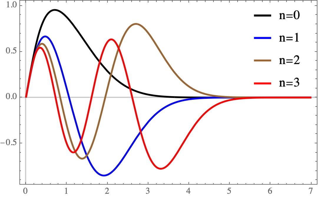
(a) Eigenfunctions $\psi_{h,n}^{-}(x,m,\alpha)$ vs $x$ for $m=1$ and $\alpha=-\frac{1}{2}$ and $n=0,1,2,3$

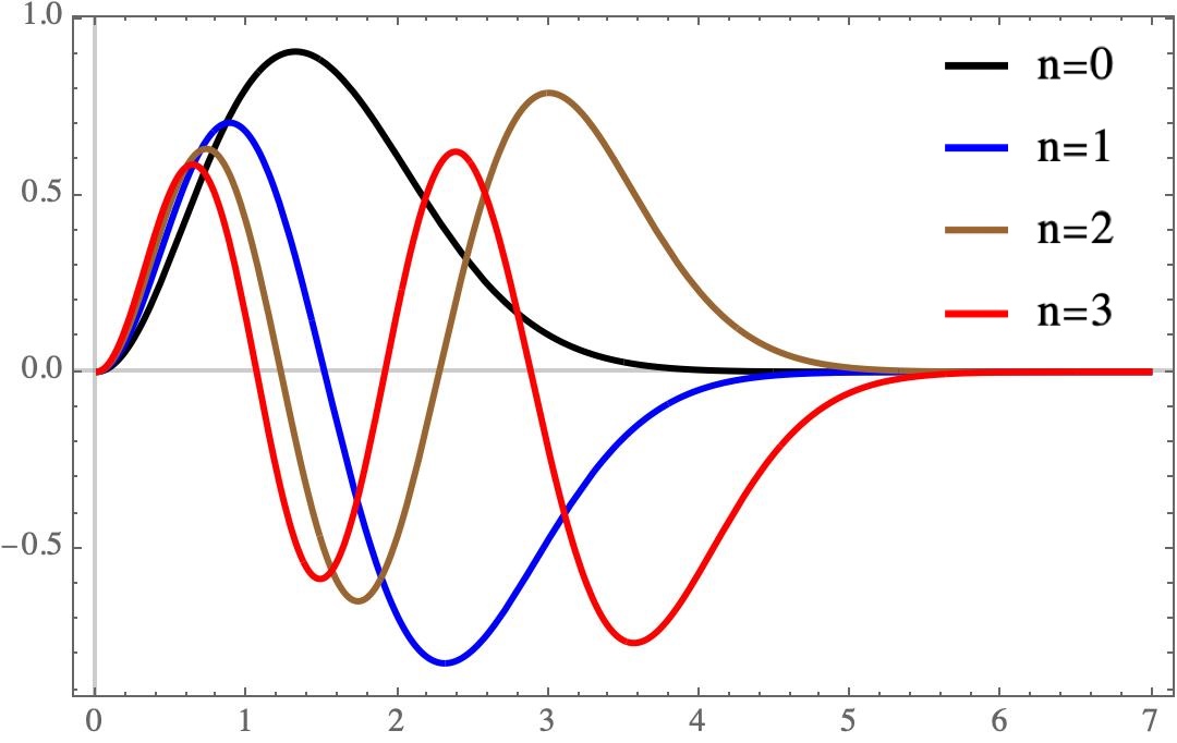
(b) Eigenfunctions $\psi_{h,n}^{-}(x,m,\alpha)$ vs $x$ for $m=1$ and $\alpha=\frac{1}{2}$ and $n=0,1,2,3$

Figure 1: Eigenfunctions for RE Half-Line oscillator.

m	$\mathbf{V_{h}^{-}(x,m,-\frac{1}{2})}$	$\mathbf{V_{h}^{-}(x,m,\frac{1}{2})}$
0	$\frac{x^{2}\omega_{x}^{2}}{4}-\omega_{x}$	$\frac{x^{2}\omega_{x}^{2}}{4}+\frac{2}{x^{2}}-\omega_{x}$
1	$\frac{x^{2}\omega_{x}^{2}}{4}+\frac{4\omega_{x}}{x^{2}\omega_{x}+1}-\frac{8\omega_{x}}{\left(x^{2}\omega_{x}+1\right)^{2}}-\omega_{x}$	$\frac{x^{2}\omega_{x}^{2}}{4}+\frac{4\omega_{x}}{x^{2}\omega_{x}+3}-\frac{24\omega_{x}}{\left(x^{2}\omega_{x}+3\right)^{2}}+\frac{2}{x^{2}}-\omega_{x}$
2	$\frac{x^{2}\omega_{x}^{2}}{4}+\frac{192x^{2}\omega_{x}^{2}}{\left(x^{4}\omega_{x}^{2}+6x^{2}\omega_{x}+3\right)^{2}}+\frac{8\left(x^{2}\omega_{x}^{2}-3\omega_{x}\right)}{x^{4}\omega_{x}^{2}+6x^{2}\omega_{x}+3}-\omega_{x}$	$\frac{x^{2}\omega_{x}^{2}}{4}+\frac{320x^{2}\omega_{x}^{2}}{\left(x^{4}\omega_{x}^{2}+10x^{2}\omega_{x}+15\right)^{2}}+\frac{8\left(x^{2}\omega_{x}^{2}-5\omega_{x}\right)}{x^{4}\omega_{x}^{2}+10x^{2}\omega_{x}+15}+\frac{2}{x^{2}}-\omega_{x}$
3	$\frac{x^{2}\omega_{x}^{2}}{4}+\frac{12\left(x^{4}\omega_{x}^{3}+45\omega_{x}\right)}{x^{6}\omega_{x}^{3}+15x^{4}\omega_{x}^{2}+45x^{2}\omega_{x}+15}-\frac{2160\left(3x^{4}\omega_{x}^{3}+10x^{2}\omega_{x}^{2}+5\omega_{x}\right)}{\left(x^{6}\omega_{x}^{3}+15x^{4}\omega_{x}^{2}+45x^{2}\omega_{x}+15\right)^{2}}-\omega_{x}$	$\frac{x^{2}\omega_{x}^{2}}{4}+\frac{12\left(x^{4}\omega_{x}^{3}+49\omega_{x}\right)}{x^{6}\omega_{x}^{3}+21x^{4}\omega_{x}^{2}+105x^{2}\omega_{x}+105}-\frac{1008\left(11x^{4}\omega_{x}^{3}+70x^{2}\omega_{x}^{2}+105\omega_{x}\right)}{\left(x^{6}\omega_{x}^{3}+21x^{4}\omega_{x}^{2}+105x^{2}\omega_{x}+105\right)^{2}}+\frac{2}{x^{2}}-\omega_{x}$

Table 1: Potentials $V^{-}_{h}(x,m,\alpha)$ (which are only valid for $x>0$) for different $m$ when $\alpha$ equals $-\frac{1}{2}$ and $\frac{1}{2}$ respectively .

m	$\mathbf{\psi_{h,n}^{-}(x,m,-\frac{1}{2})}$	$\mathbf{\psi_{h,n}^{-}(x,m,\frac{1}{2})}$
0	$xe^{-\frac{\omega_{x}x^{2}}{4}}L_{n}^{(\frac{1}{2})}\left(\frac{\omega_{x}}{2}x^{2}\right)$	$x^{2}e^{-\frac{\omega_{x}x^{2}}{4}}L_{n}^{(\frac{3}{2})}\left(\frac{\omega_{x}}{2}x^{2}\right)$
1	$xe^{-\frac{\omega_{x}x^{2}}{4}}\left[L_{n-1}^{(\frac{1}{2})}\left(\frac{\omega_{x}}{2}x^{2}\right)+\frac{\left(\omega_{x}x^{2}+3\right)L_{n}^{(-\frac{1}{2})}\left(\frac{\omega_{x}}{2}x^{2}\right)}{\omega_{x}x^{2}+1}\right]$	$x^{2}e^{-\frac{\omega_{x}x^{2}}{4}}\left[L_{n-1}^{(\frac{3}{2})}\left(\frac{\omega_{x}}{2}x^{2}\right)+\frac{\left(\omega_{x}x^{2}+5\right)L_{n}^{(\frac{1}{2})}\left(\frac{\omega_{x}}{2}x^{2}\right)}{\omega_{x}x^{2}+3}\right]$
2	$xe^{-\frac{\omega_{x}x^{2}}{4}}\Bigg{[}L_{n-1}^{(\frac{1}{2})}\left(\frac{\omega_{x}}{2}x^{2}\right)+\frac{\left(2\omega_{x}x^{2}\left(\frac{\omega_{x}}{2}x^{2}+5\right)+15\right)L_{n}^{(-\frac{1}{2})}\left(\frac{\omega_{x}}{2}x^{2}\right)}{2\omega_{x}x^{2}\left(\frac{\omega_{x}}{2}x^{2}+3\right)+3}\Bigg{]}$	$x^{2}e^{-\frac{\omega_{x}x^{2}}{4}}\Bigg{[}L_{n-1}^{(\frac{3}{2})}\left(\frac{\omega_{x}}{2}x^{2}\right)+\frac{\left(2\omega_{x}x^{2}\left(\frac{\omega_{x}}{2}x^{2}+7\right)+35\right)L_{n}^{(\frac{1}{2})}\left(\frac{\omega_{x}}{2}x^{2}\right)}{2\omega_{x}x^{2}\left(\frac{\omega_{x}}{2}x^{2}+5\right)+15}\Bigg{]}$
3	$xe^{-\frac{\omega_{x}x^{2}}{4}}\Bigg{[}L_{n-1}^{(\frac{1}{2})}\left(\frac{\omega_{x}}{2}x^{2}\right)+\frac{\left(4\omega_{x}^{3}x^{6}+42\omega_{x}^{2}x^{4}+105\omega_{x}x^{2}+105\right)L_{n}^{(-\frac{1}{2})}\left(\frac{\omega_{x}}{2}x^{2}\right)}{4\omega_{x}^{3}x^{6}+30\omega_{x}^{2}x^{4}+45\omega_{x}x^{2}+15}\Bigg{]}$	$x^{2}e^{-\frac{\omega_{x}x^{2}}{4}}\Bigg{[}L_{n-1}^{(\frac{3}{2})}\left(\frac{\omega_{x}}{2}x^{2}\right)+\frac{\left(\omega_{x}x^{2}\left(2\omega_{x}^{2}x^{4}+27\omega_{x}x^{2}+189\right)+315\right)L_{n}^{(\frac{1}{2})}\left(\frac{\omega_{x}}{2}x^{2}\right)}{4\omega_{x}^{3}x^{6}+42\omega_{x}^{2}x^{4}+105\omega_{x}x^{2}+105}\Bigg{]}$

Table 2: Eigenfunctions corresponding to $V_{h}^{-}(x,m,\alpha)$ for different $m$ and $\alpha$ equals $-\frac{1}{2}$ and $\frac{1}{2}$ respectively.

3 Two-Dimensional Anisotropic Harmonic Oscillator

In this section, we use the results discussed in the last section and construct the two-dimensional anisotropic harmonic oscillator RE potentials and the exact eigenfunctions. There are three possible rational extensions of the 2D anisotropic harmonic oscillator, namely

1. $2$D-Full-line oscillator

2. $2$D-Truncated oscillator and

3. combination of $1$D-Full-line and $1$D-Half-line oscillator.

3.1 $2$D-Full-line oscillator

Consider the $2$D-anisotropic harmonic oscillator potential defined on the full $xy$-plane

$$V^{+}(x,y)=\frac{1}{4}\omega_{x}^{2}x^{2}+\frac{1}{4}\omega_{y}^{2}y^{2};\quad-\infty<x<\infty,-\infty<y<\infty$$ (3.1)

with the eigenfunctions and the eigenvalues

$$\psi_{n_{1},n_{2}}^{+}(x,y) \propto \psi_{n_{1}}^{+}(x)\psi_{n_{2}}^{+}(y)$$ (3.2)

$$\propto e^{-\frac{\omega_{x}x^{2}+\omega_{y}y^{2}}{4}}H_{n_{1}}\left(\sqrt{\frac{\omega_{x}}{2}}x\right)H_{n_{2}}\left(\sqrt{\frac{\omega_{y}}{2}}y\right)\;\quad n_{1},n_{2}=0,1,2,\cdots,$$

and

$$E^{+}_{n_{1},n_{2}}=E^{+}_{n_{1}}+E^{+}_{n_{2}}$$ (3.3)

respectively where $E^{+}_{n}$ is given by Eq. (2.17). The seedless function along each axis can be constructed by replacing the frequencies in the eigenfunctions of conventional potential (3.2) with imaginary frequencies and the integers $n_{1}$ and $n_{2}$ are replaced by $m_{1}$ and $m_{2}$ respectively. This way one gets $(m_{1},\;m_{2})$-dependent seedless function defined as

$$\phi_{m_{1},m_{2}}(x,y)=\prod_{k=1}^{2}\phi_{m_{k}}(x_{k})\quad\text{where}\quad(x_{1},x_{2})\rightarrow(x,y)\,.$$ (3.4)

In this way, we get the seedless function

$$\phi_{m_{1},m_{2}}(x,y)\propto e^{\frac{\omega_{x}\;x^{2}+\omega_{y}\;y^{2}}{4}}H_{m_{1}}\left(i\sqrt{\frac{\omega_{x}}{2}}x\right)H_{m_{2}}\left(i\sqrt{\frac{\omega_{y}}{2}}y\right)$$ (3.5)

and this gives $Q_{2}=0$ (see the Eq. (B.6) in the Appendix B) and therefore the SUSY partners of $V^{+}(x)$, i.e. the RE potentials $V^{-}(x,y,m_{1},m_{2})$ are given by adding the individual partner potentials as given in (2.4). In particular

$$V^{-}(x,y,m_{1},m_{2})=V^{-}(x,m_{1})+V^{-}(y,m_{2})\,$$ (3.6)

where $m_{1}$ and $m_{2}$ are both positive even integers. The ground and the excited state eigenfunctions are given by

$$\begin{split}\psi^{-}_{0,0}(x,y,m_{1},m_{2})&=\phi_{m_{1}}^{-1}(x)\phi_{m_{2}}^{-1}(y),\\ \mbox{and}\quad\psi^{-}_{n_{1}+1,n_{2}+1}(x,y,m_{1},m_{2})&=\psi^{-}_{n_{1}+1}(x,m_{1})\psi^{-}_{n_{2}+1}(y,m_{2})\;,\qquad n_{1},n_{2}=0,1,2,\cdots\\ \end{split}$$ (3.7)

respectively while the energy eigenvalues are given by

$$E_{n_{1}+1,n_{2}+1,m_{1},m_{2}}^{-} =\left[\left(n_{1}+m_{1}+1\right)\omega_{x}+\left(n_{2}+m_{2}+1\right)\omega_{y}\right]\quad\text{and}\quad E_{0,0,m_{1},m_{2}}^{-}=0.$$ (3.8)

Notice that the spectrum of the extended potential is strictly isospectral to the conventional starting potential and hence the form of the degeneracy will be identical to that of the $2D$-anisotropic harmonic oscillator potential (see for example [31]). Notice that the degeneracy occurs if the ratio of the two frequencies $\omega_{x}$ and $\omega_{y}$ is a rational number.

3.2 2D-Half-Line Oscillator

The half-line oscillator is defined in the region $(x,y)\in(0,\infty)\times(0,\infty)$. The potential is given by

$$V^{+}_{h}(x,y)=\begin{cases}\frac{1}{4}\omega_{x}^{2}x^{2}+\frac{1}{4}\omega_{y}^{2}y^{2}&\text{for}(x,y)\in(0,\infty)\times(0,\infty),\\ \infty&\text{otherwise}\end{cases}$$

Using the results obtained for the one-dimensional case in the previous section i.e. equation (2.9), the eigenfunctions for this potential are given by

$$\psi_{h,n_{1},n_{2}}^{+}(x,y,\alpha,\beta)\propto x^{\alpha+\frac{1}{2}}y^{\beta+\frac{1}{2}}e^{-\frac{\omega_{x}x^{2}+\omega_{y}y^{2}}{4}}L_{n_{1}}^{(\alpha)}\left(\frac{\omega_{x}}{2}x^{2}\right)L_{n_{2}}^{(\beta)}\left(\frac{\omega_{y}}{2}y^{2}\right);\quad n_{1},n_{2}=0,1,2,\cdots$$ (3.9)

where, $\beta=\pm\frac{1}{2}$ is another parameter for the potential defined along the $y$ direction. The seedless solution $\phi_{h,m_{1},m_{2}}(x,y,\alpha,\beta)$ corresponding to this potential can be easily constructed by replacing $(n_{1},n_{2})\rightarrow(m_{1},m_{2})$ and $(\omega_{x},\omega_{y})\rightarrow(-\omega_{x},-\omega_{y})$ in $\psi_{n_{1},n_{2}}^{+}(x,y,\alpha,\beta)$ and is given by

$$\phi_{h,m_{1},m_{2}}(x,y,\alpha,\beta)\propto x^{\alpha+\frac{1}{2}}y^{\beta+\frac{1}{2}}e^{\big{(}\frac{\omega_{x}x^{2}+\omega_{y}y^{2}}{4}\big{)}}L_{m_{1}}^{(\alpha)}\left(-\frac{\omega_{x}}{2}x^{2}\right)L_{m_{2}}^{(\beta)}\left(-\frac{\omega_{y}}{2}y^{2}\right);\qquad m_{1},m_{2}=0,1,2,\cdots\,.$$ (3.10)

The corresponding energy eigenvalues of the Hamiltonian $H_{h}^{+}(x,y)$ is obtained using $V^{+}_{h}(x,y)-\epsilon_{h,m_{1},m_{2}}$ as

$$E^{+}_{h,n_{1},n_{2},\alpha,\beta}=[(2n_{1}+\alpha+1)\omega_{x}+(2n_{2}+\beta+1)\omega_{y}]-\epsilon_{h,m_{1},m_{2}},$$ (3.11)

where $\epsilon_{h,m_{1},m_{2}}=-[(2m_{1}+\alpha+1)\omega_{x}+(2m_{2}+\beta+1)\omega_{y}]$ is the factorization energy corresponding to the seedless function $\phi_{h,m_{1},m_{2}}(x,y,\alpha,\beta)$. There are four possible combinations of the parameters $\alpha$ and $\beta$ (i.e. $\alpha=\beta=\pm 1/2$ and $\alpha=1/2,\beta=-1/2$ and $\alpha=-1/2,\beta=1/2$), out of which the case $\alpha=1/2,\beta=-1/2$ and $\alpha=-1/2,\beta=1/2$ are equivalent. Thus effectively we have three forms of the RE potentials which we now discuss one by one.

Case (a) For $\alpha=\beta=1/2$

The form of the extended potential, the corresponding eigenfunctions and the energy eigenvalues are given by

$$V_{h}^{-}(x,y,m_{1},m_{2},\frac{1}{2}) =V_{h}^{-}(x,m_{1},\frac{1}{2})+V_{h}^{-}(y,m_{2},\frac{1}{2})$$ (3.12)

$$\psi_{h,n_{1},n_{2}}^{-}(x,y,m_{1},m_{2},\frac{1}{2}) \propto\psi^{-}_{n_{1}}(x,m_{1},\frac{1}{2})\psi^{-}_{n_{2}}(y,m_{2},\frac{1}{2})$$ (3.13)

$$\mbox{and}\quad E_{h,n_{1},n_{2}}^{-}(m_{1},m_{2},\frac{1}{2}) =\left[\left(2n_{1}+2m_{1}+3\right)\omega_{x}+\left(2n_{2}+2m_{2}+3\right)\omega_{y}\right]\,$$ (3.14)

respectively. Here the potentials $V_{h}^{-}(x,m_{1},\frac{1}{2})$ and $V_{h}^{-}(y,m_{2},\frac{1}{2})$ and the eigenfunctions $\psi^{-}_{n_{1}}(x,m_{1},\frac{1}{2})$ and $\psi^{-}_{n_{2}}(y,m_{2},\frac{1}{2})$ can be easily obtained from Eqs. (2.13) and (2.15) respectively. In the special case of the isotropic oscillator (i.e. $\omega_{x}=\omega_{y}$) the results for the RE potential (where $m_{1}=m_{2}=m$(say)), are the same as those obtained in [21] for $D=2$ and are valid for all positive values of $m$.

Case (b) For $\alpha=\beta=-1/2$

In this case, the form of potential with the corresponding energy eigenfunctions and the energy eigenvalues are

$$V_{h}^{-}(x,y,m_{1},m_{2},-\frac{1}{2}) =V_{h}^{-}(x,m_{1},-\frac{1}{2})+V_{h}^{-}(y,m_{2},-\frac{1}{2})$$ (3.15)

$$\psi_{h,n_{1},n_{2}}^{-}(x,y,m_{1},m_{2},-\frac{1}{2}) \propto\psi^{-}_{h,n_{1}}(x,m_{1},-\frac{1}{2})\psi^{-}_{h,n_{2}}(y,m_{2},-\frac{1}{2})$$ (3.16)

$$\mbox{and}\quad E_{h,n_{1},n_{2}}^{-}(m_{1},m_{2},\frac{1}{2}) =\left[\left(2n_{1}+2m_{1}+1\right)\omega_{x}+\left(2n_{2}+2m_{2}+1\right)\omega_{y}\right]\,.$$ (3.17)

Here the potentials $V_{h}^{-}(x,m_{1},-\frac{1}{2})$ and $V_{h}^{-}(y,m_{2},-\frac{1}{2})$ and the eigenfunctions $\psi^{-}_{n_{1}}(x,m_{1},-\frac{1}{2})$ and $\psi^{-}_{n_{2}}(y,m_{2},-\frac{1}{2})$ can be easily obtained from Eqs. (2.14) and (2.15) respectively.

Case (c) For $\alpha=\frac{1}{2}$ and $\beta=-\frac{1}{2}$

Similar to the above cases, the potential, the eigenfunctions and the energy eigenvalues are given by

$$V_{h}^{-}(x,y,m_{1},m_{2},\frac{1}{2},-\frac{1}{2}) =V_{h}^{-}(x,m_{1},\frac{1}{2})+V_{h}^{-}(y,m_{2},-\frac{1}{2})$$ (3.18)

$$\psi_{h,n_{1},n_{2}}^{-}(x,y,m_{1},m_{2},\frac{1}{2},-\frac{1}{2}) \propto\psi^{-}_{h,n_{1}}(x,m_{1},\frac{1}{2})\psi^{-}_{h,n_{2}}(y,m_{2},-\frac{1}{2})$$ (3.19)

$$\mbox{and}\quad E_{h,n_{1},n_{2}}^{-}(m_{1},m_{2},\frac{1}{2},-\frac{1}{2}) =\left[\left(2n_{1}+2m_{1}+3\right)\omega_{x}+\left(2n_{2}+2m_{2}+1\right)\omega_{y}\right]\,$$ (3.20)

The form of the degeneracy in this case is similar to the full line case and hence identical to that of the $2D$-anisotropic harmonic oscillator potential (see for example [31]). Notice that the degeneracy occurs when the ratio $\frac{\omega_{x}}{\omega_{y}}$ is a rational number.

3.3 One Full-Line and One Half-Line Oscillator

This two dimensional anisotropic harmonic oscillator is defined with one coordinate spanning the entire real line (say along the $x-$axis) and the other truncated at zero (say along the $y-$axis) as

$$V^{+}_{fh}(x,y)=\begin{cases}\frac{1}{4}\omega_{x}^{2}x^{2}+\frac{1}{4}\omega_{y}^{2}y^{2}&\text{for }y>0;-\infty<x<\infty,\\ \infty&\text{for }y\leq 0\end{cases}$$

The rational extension for this combined full-line and a half-line oscillators can be easily constructed by using the known results as given by Eqs. (2.4), (2.13) and (2.14) respectively. As already discussed in the previous section, while in the case of the full line oscillator there is one extra bound state, however in the case of the half-line oscillator (which is $\beta$ dependent), there is no extra bound state. The general form of the extended potential is given as

$$V^{-}_{fh}(x,y,m_{1},m_{2},\beta)=V^{-}(x,m_{1})+V^{-}_{h}(y,m_{2},\beta),$$ (3.21)

here $m_{1}=0,2,4,\cdots$, $m_{2}=0,1,2,3,\cdots$ and $\beta=\pm 1/2$. The corresponding ground and the excited state eigenfunctions are

$$\psi^{-}_{fh,0,0}(x,y,m_{1},m_{2},\beta)\propto\psi^{-}_{0}(x,m_{1})\psi^{-}_{h,0}(y,m_{2},\beta)$$ (3.22)

and

$$\psi^{-}_{fh,n_{1}+1,n_{2}}(x,y,m_{1},m_{2},\beta)\propto\psi^{-}_{n_{1}+1}(x,m_{1})\psi^{-}_{h,n_{2}}(y,m_{2},\beta);$$ (3.23)

respectively. Here $n_{1}=0,1,2,\cdots$ and $n_{2}=1,2,3,\cdots$. The corresponding expressions for the ground and the excited state energy eigenvalues are

$$E^{-}_{fh,0,0}(m_{2},\beta)=2(m_{2}+\beta+1)\omega_{y}.$$ (3.24)

and

$$E^{-}_{fh,n_{1}+1,n_{2}}(m_{1},m_{2},\beta) = E^{+}_{n_{1}}(m_{1})+E^{+}_{h,n_{2}}(m_{2},\beta)$$ (3.25)

$$= (n_{1}+m_{1}+1)\omega_{x}+2(n_{2}+m_{2}+\beta+1)\omega_{y}$$

respectively. The explicit expressions for the extended potentials and the corresponding energy eigenvalues and eigenfunctions in case $\beta=\pm 1/2$ are as follows:

Case (a) For $\beta=\frac{1}{2}$

In this case, we use the expressions of $V^{-}(x,m_{1})$, $V_{h}^{-}(y,m_{2},\frac{1}{2})$ and $V^{-}_{h}(y,m_{2},-1/2)$ from Eqs. (2.4), (2.13) and (2.14) respectively, and get

$$V^{-}_{fh}(x,y,m_{1},m_{2},1/2) =V^{-}(x,m_{1})+V_{h}^{-}(y,m_{2},\frac{1}{2})$$ (3.26)

The corresponding ground and the excited state eigenfunctions and the the corresponding energy eigenvalues are given by

$$\psi^{-}_{fh,0,0}(m_{1},m_{2},\frac{1}{2}) \propto\psi^{-}_{0}(x,m_{1})\psi^{-}_{h,0}(y,m_{2},\frac{1}{2})$$ (3.27)

$$\psi^{-}_{n_{1}+1,n_{2}}(m_{1},m_{2},\frac{1}{2}) \propto\psi^{-}_{n_{1}+1}(x,m_{1})\psi^{-}_{h,n_{2}}(y,m_{2},\frac{1}{2})$$ (3.28)

and

$$E^{-}_{0,0}(m_{1},m_{2},\frac{1}{2}) =\left(2m_{2}+3\right)\omega_{y}$$ (3.29)

$$E^{-}_{n_{1}+1,n_{2}}(m_{1},m_{2},\frac{1}{2}) =\left(n_{1}+2m_{1}+1\right)\omega_{x}+\left(2n_{2}+2m_{2}+3\right)\omega_{y}$$ (3.30)

respectively.

Case (b) For $\beta=-\frac{1}{2}$

Here the form of the extended potential is given by

$$V^{-}_{fh}(x,y,m_{1},m_{2},-1/2) =V^{-}(x,m_{1})+V_{h}^{-}(y,m_{2},-\frac{1}{2})$$ (3.31)

The corresponding ground and the excited state eigenfunctions and the energy eigenvalues are

$$\psi^{-}_{fh,0,0}(m_{1},m_{2},-\frac{1}{2}) \propto\psi^{-}_{0}(x,m_{1})\psi^{-}_{h,0}(y,m_{2},-\frac{1}{2})$$ (3.32)

$$\psi^{-}_{n_{1}+1,n_{2}}(m_{1},m_{2},-\frac{1}{2}) \propto\psi^{-}_{n_{1}+1}(x,m_{1})\psi^{-}_{h,n_{2}}(y,m_{2},-\frac{1}{2})$$ (3.33)

and

$$E^{-}_{0,0}(m_{1},m_{2},-\frac{1}{2}) =\left(2m_{2}+1\right)\omega_{y}$$ (3.34)

$$E^{-}_{n_{1}+1,n_{2}}(m_{1},m_{2},-\frac{1}{2}) =\left(n_{1}+2m_{1}+1\right)\omega_{x}+\left(2n_{2}+2m_{2}+1\right)\omega_{y}$$ (3.35)

respectively.

One point worth mentioning here. As seen above, when both the oscillators are on the full line or both on the half line, the degeneracy for given $m_{1},m_{2}$ essentially comes from the factor $n_{1}\omega_{x}+n_{2}\omega_{y}$. However, when one oscillator is on the full line and the other is on the half-line then for a given $m_{1},m_{2}$, the degeneracy essentially comes from the factor $n_{1}\omega_{x}+2n_{2}\omega_{y}$, which is different from the two above cases. As a result, for a given rational value of $\frac{\omega_{x}}{\omega_{y}}$, the degeneracy will be different in this case in contrast to the other two cases.

4 Three-Dimensional Anharmonic Harmonic Oscillator

Similar to the 2D anisotropic case, generalization to arbitrary $D$ dimensions is straight forward. For example, using the seedless function for each potential $V^{+}(x_{k})$ along a given axis (full line or half line), one can construct a $(m_{1},m_{2},m_{3})$-dependent three dimensional RE anisotropic harmonic oscillator potential $V^{-}(x,y,z,m_{1},m_{2},m_{3})$ by starting from the known anisotropic three dimensional potential $V^{+}(x,y,z)$, whose expression is given by (B.10) with zero value of $Q_{3}$ in (B.6). The corresponding eigenfunctions and the energy eigenvalues are given by (B.11) and (B.12) respectively.

In the case of all three half-line oscillators, with all three frequencies equal, there are two possible forms of the extended potentials corresponding to $\alpha=\pm\frac{1}{2}$. For $\alpha=\frac{1}{2}$ the extended potential obtained in polar coordinates reduces to the same form as already obtained in [21] for $D$-dimensional isotropic harmonic oscillator with $D=3$ and $l=1$, except for an additional constant of $-\frac{3}{2}\omega$ in [21]. But for $\alpha=-1/2$, we get another form of the extended isotropic potential. The form of this potential with their solutions can easily be obtained using the results obtained for the one-dimensional case and using Eqs. (2.14), (2.15) and (2.17). It is then worthwhile to consider the problem of the 3-dimensional anisotropic oscillator in case two of the three frequencies are the same and obtain their rational extension.

4.1 Full-Line Oscillator with two equal frequencies

Consider the following anisotropic potential defined on the full-line

$$V^{+}(x,y,z)=\frac{1}{4}\omega^{2}(x^{2}+y^{2})+\frac{1}{4}\omega_{z}^{2}z^{2};\quad-\infty<x,y,z<\infty$$ (4.1)

where $\omega_{x}=\omega_{y}=\omega$. In this case the above potential can be written in the $r-z$ co-ordinates as

$$V^{+}(r,z)=\frac{1}{4}\omega^{2}r^{2}+\frac{1}{4}\omega_{z}^{2}z^{2}\,$$ (4.2)

where $r^{2}=x^{2}+y^{2}$. The form of the Schrödinger equation in the cylindrical co-ordinates ($r,\phi,z$) is

$$\left[-\left(\frac{1}{r}\frac{\partial}{\partial r}r\frac{\partial}{\partial r}+\frac{1}{r^{2}}\frac{\partial^{2}}{\partial\phi^{2}}+\frac{\partial^{2}}{\partial z^{2}}\right)+V^{+}(r,z)\;\right]\psi^{+}(r,\phi,z)=E\psi^{+}(r,\phi,z),$$ (4.3)

where $\psi^{+}(r,\phi,z)$ is the eigenfunction and $E$ is the energy eigenvalue corresponding to the potential $V^{+}(r,z)$. One can easily solve the Eq. (4.3) by assuming

$$\psi^{+}(r,\phi,z)=\frac{e^{i\gamma\phi}\zeta(r,z)}{r^{\frac{1}{2}}}\,.$$ (4.4)

where

$$\zeta(r,z)=R(r)Z(z)\,.$$ (4.5)

One can show that in this case $\zeta(r,z)$ satisfies the equation

$$\left[-\frac{\partial^{2}}{\partial r^{2}}-\frac{\partial^{2}}{\partial z^{2}}+V^{+}_{eff}(r,z)\right]\zeta(r,z)=E\;\zeta(r,z),$$ (4.6)

where the effective potential $V^{+}_{eff}(r,z)$ is given by

$$V^{+}_{eff}(r,z)=V^{+}(r,z)+\frac{\gamma^{2}-1/4}{r^{2}}\quad\text{with}\quad\gamma=0,\pm 1,\pm 2,\cdots\,.$$ (4.7)

The functions $R(r)$ and $Z(z)$ can be shown to be

$$R(r)\rightarrow R_{n_{1}}(r)\propto r^{|\gamma|+\frac{1}{2}}e^{-\frac{\omega}{4}r^{2}}L_{n_{1}}^{|\gamma|}(\frac{1}{2}\omega r^{2});n_{1}=0,1,2,\cdots$$ (4.8)

and

$$Z(z)\rightarrow Z_{n_{2}}(z)\propto e^{-\frac{\omega_{z}z^{2}}{4}}H_{n_{2}}(\sqrt{\frac{\omega_{z}}{2}}z);n_{2}=0,1,2,\cdots$$ (4.9)

respectively. The corresponding energy eigenvalues $E$ turn out to be

$$E\rightarrow E_{n_{1},n_{2}}=(2n_{1}+|\gamma|+1)\omega+\left(n_{2}+\frac{1}{2}\right)\omega_{z}\,.$$ (4.10)

Thus the energy eigenvalues for the Hamiltonian $H^{+}(r,z)=V^{+}(r,z)-\epsilon_{m_{1},m_{2}}$ are

$$E^{+}_{n_{1},n_{2}}=E_{n_{1},n_{2}}-\epsilon_{m_{1},m_{2}}=2(n_{1}+m_{1}+|\gamma|+1)\omega+(n_{2}+m_{2}+1)\omega_{z}.$$ (4.11)

Now one can easily construct the corresponding RE potential $V_{eff}^{+}(r,z)$ by defining the seedless functions $\phi_{m_{1}}(r)$ and $\phi_{m_{2}}(z)$, by replacing $n_{1}\rightarrow m_{1}$, $\omega\rightarrow-\omega$ and $n_{2}\rightarrow m_{2}$, $\omega_{z}\rightarrow-\omega_{z}$ in the expressions for $R_{n_{1}}(r)$ and $Z_{n_{2}}(z)$ respectively. We obtain

$$\begin{split}\phi_{m_{1}}(r)&\propto r^{|\gamma|+\frac{1}{2}}e^{\frac{\omega}{4}r^{2}}L_{m_{1}}^{|\gamma|}\left(-\frac{1}{2}\omega r^{2}\right);\qquad m_{1}=0,1,2\cdots\\ \phi_{m_{2}}(z)&\propto e^{\frac{\omega_{z}}{4}z^{2}}\mathcal{H}_{m_{2}}\left(\sqrt{\frac{\omega_{z}}{2}}z\right);\qquad m_{2}=0,2,4\cdots\quad\text{Since $z$ axis is full line.}\end{split}$$ (4.12)

Thus the combined seedless function corresponding to the wavefunction $\zeta(r,z)$ will be

$$\phi_{m_{1},m_{2}}(r,z)=\phi_{m_{1}}(r)\phi_{m_{2}}(z)$$ (4.13)

and the operators $A$ and $A^{\dagger}$ in term of $\phi_{m_{1},m_{2}}(r,z)$ are given by

$$\begin{split}A&=\frac{\partial}{\partial r}+\frac{\partial\log(\phi_{m_{1},m_{2}}(r,z))}{\partial r}+i\frac{\partial}{\partial z}+i\frac{\partial\log\phi_{m_{1},m_{2}}(r,z)}{\partial z}\\ \mbox{and}\quad A^{\dagger}&=-\frac{\partial}{\partial r}+\frac{\partial\log(\phi_{m_{1},m_{2}}(r,z))}{\partial r}+i\frac{\partial}{\partial z}-i\frac{\partial\log\phi_{m_{1},m_{2}}(r,z)}{\partial z}\end{split}$$ (4.14)

respectively. The RE potential $V_{eff}^{-}(m_{1},m_{2},r,z)$ with the corresponding eigenfunctions $\zeta_{n_{1},n_{2}}^{-}(r,z,m_{1},m_{2})$ and energy eigenvalues $E^{-}_{n_{1},n_{2}}(m_{1},m_{2})$ corresponding to the potential $V_{eff}(r,z)$ are

$$V_{eff}^{-}(m_{1},m_{2},r,z) =\frac{1}{4}\omega^{2}r^{2}+\frac{\gamma^{2}-\frac{1}{4}}{r^{2}}+\frac{2|\gamma|}{r^{2}}-(2m+1)\omega+\frac{1}{r^{2}}$$

$$\quad+\frac{2r^{2}\omega^{2}L_{m_{1}-1}^{(|\gamma|+1)}\left(-\frac{\omega r^{2}}{2}\right){}^{2}}{L_{m_{1}}^{(|\gamma|)}\left(-\frac{\omega r^{2}}{2}\right){}^{2}}$$

$$\quad+\frac{\omega\left(\left(2|\gamma|+r^{2}\omega\right)L_{m_{1}-1}^{(|\gamma|+1)}\left(-\frac{\omega r^{2}}{2}\right)-r^{2}\omega L_{m-2}^{(|\gamma|+2)}\left(-\frac{\omega r^{2}}{2}\right)\right)}{L_{m_{1}}^{(|\gamma|)}\left(-\frac{\omega r^{2}}{2}\right)}$$

$$\quad+\frac{1}{2}\omega_{z}^{2}z^{2}-2\left[\frac{\mathcal{H}_{m_{2}}^{\prime\prime}\left(\sqrt{\frac{\omega_{z}}{2}}z\right)}{\mathcal{H}_{m_{2}}\left(\sqrt{\frac{\omega_{z}}{2}}z\right)}-\left[\frac{\mathcal{H}_{m_{2}}^{\prime}\left(\sqrt{\frac{\omega_{z}}{2}}z\right)}{\mathcal{H}_{m_{2}}\left(\sqrt{\frac{\omega_{z}}{2}}z\right)}\right]^{2}+\frac{\omega_{z}}{2}\right]$$

$$\zeta_{n_{1},n_{2}+1}^{-}(r,z,m_{1},m_{2}) \propto r^{|\gamma|+\frac{3}{2}}e^{-\frac{\omega r^{2}}{4}}\frac{\hat{L}_{n_{1},m_{1}}^{\gamma}\left(\frac{1}{2}\omega r^{2}\right)}{L_{m_{1}}^{\gamma}\left(-\frac{1}{2}\omega r^{2}\right)}\;e^{-\frac{\frac{\omega_{z}}{2}z^{2}}{2}}\frac{\hat{H}_{n_{z}+1,m_{2}}\left(\sqrt{\frac{\omega_{z}}{2}}z\right)}{\mathcal{H}_{m_{2}}\left(\sqrt{\frac{\omega_{z}}{2}}z\right)}$$

$$E^{-}_{n_{1},n_{2}+1}(m_{1},m_{2}) =2(n_{1}+m_{1}+|\gamma|+1)\omega+\left(n_{2}+m_{2}+1\right)\omega_{z}$$ (4.15)

with the ground state eigenfunctions and the energy eigenvalues

$$\zeta_{0,0}^{-}(r,z,m_{1},m_{2}) \propto r^{|\gamma|+\frac{3}{2}}\frac{e^{-\frac{\omega r^{2}}{4}}L_{\text{m1}}^{|\gamma|+1}\left(\frac{1}{2}\omega\left(-r^{2}\right)\right)}{L_{m_{1}}^{|\gamma|}\left(-\frac{1}{2}\omega r^{2}\right)}\times\frac{e^{-\frac{\omega_{z}\;z^{2}}{4}}}{\mathcal{H}_{m_{2}}\left(\sqrt{\frac{\omega_{z}}{2}}z\right)}$$

$$\mbox{and}\quad E^{-}_{0,0,m_{1},m_{2}} = 2(m_{1}+|\gamma|+1)\omega$$ (4.16)

respectively, where, the prime over pseudo-Hermite polynomial $\mathcal{H}_{m}(\sqrt{\frac{\omega_{z}}{2}}z)$ denotes derivatives with respect to $z$. The RE potential is isospectral but not strictly isospectral to $V^{+}$ as there is additional bound state along $z$-axis. The form of the degeneracy is therefore the same for the RE potential and $V^{+}$. The degeneracy in the RE case (for given $m_{1},m_{2}$) occurs when the ratio of $\omega$ and $\omega_{z}$ is a rational number. The form of the degeneracy in this case is similar to the full line case and hence identical to that of the $2D$-anisotropic harmonic oscillator potential (see for example [31]). Notice that the degeneracy occurs when the ratio $\frac{\omega_{x}}{\omega_{y}}$ is a rational number.

5 Conclusions and Open Problem

In this paper, we began with the one-dimensional harmonic oscillator and derived the rational extension for the potential on the half-line. We also obtained the corresponding eigenfunctions, which are expressed in terms of Laguerre polynomials. The solutions are dependent on the parameter $\alpha=\pm\frac{1}{2}$. While the result for $\alpha=+\frac{1}{2}$ is well-known, however the case for $\alpha=-\frac{1}{2}$ is new and novel. We then extended these results to the two-dimensional anisotropic harmonic oscillator, discussing the RE potentials in the three possible cases, i.e. the full-line oscillator along both the axes, the half-line oscillator along both the axes, and a combination of the full-line oscillator on one axes and the half-line oscillator on the other. For the half-line oscillator, we found that no additional bound states exist, whereas for the full-line oscillator, an additional bound state with zero energy appears. The rational extension of the anharmonic harmonic oscillator to higher dimensions is easily done using SUSY in two, three and higher dimensions. Finally, we also considered one interesting case of three-dimensional anisotropic oscillator, where we constructed the RE potential in the case of the full line oscillator system with two equal frequencies and obtained the solution in terms of exceptional Laguerre and Hermite polynomials using cylindrical coordinates.

Now that one has obtained the RE potentials for the anisotropic harmonic oscillator potential in two and higher dimensions, one obvious question is can we add some perturbation to these potentials and still obtain the corresponding rational extension or can we generate an extended family of potentials with some perturbation corresponding to these potentials? We hope to address this question in the near future.

Appendix A: SUSY in One Dimension

The Schrödinger equation (in units $\hbar=2M=1$, where $M$ is the mass) for a system with potential $V(x)$ is represented by the equation

$$\left[-\nabla^{2}+V(x)\right]\psi_{n}(x)=E\psi_{n}(x)$$ (A.1)

or, compactly,

$$H\psi_{n}(x)=E\psi_{n}(x),$$ (A.2)

where $H$ is the second-order Hamiltonian operator. One can factorize the Hamiltonian into two linear operators $A$ (annihilation operator) and $A^{\dagger}$ (creation operator) to get two possible Hamiltonians $H^{\pm}$ as the operators are non-commutative in general.

$$\begin{split}A&=\frac{d}{dx}+W(x)\\ \text{and}\quad A^{\dagger}&=-\frac{d}{dx}+W(x)\end{split}$$ (A.3)

where $W(x)$ is the superpotential. Depending on the order of the operators, the two Hamiltonians are given by

$$H-\epsilon=\begin{cases}A^{\dagger}A=-\frac{d^{2}}{dx^{2}}+V^{-}(x)-\epsilon,&\text{say }H^{-}\\ AA^{\dagger}=-\frac{d^{2}}{dx^{2}}+V^{+}(x)-\epsilon,&\text{say }H^{+}\end{cases}$$ (A.4)

where $V^{\mp}(x)$ are the partner potentials having the expressions

$$V^{\mp}(x)=W(x)^{2}\mp W(x)^{\prime}+\epsilon$$ (A.5)

and $\epsilon$ is the factorization energy assumed less than or equal to the ground state energy $E_{0}$ of $V^{+}(x)$.

$$\left[-\frac{d^{2}}{dx^{2}}+V^{+}(x)\right]\psi_{0}^{+}(x)=E_{0}^{+}\psi_{0}^{+}(x)$$ (A.6)

and seedless eigenfunction satisfy the following equation

$$\left[-\frac{d^{2}}{dx^{2}}+V^{+}(x)\right]\phi_{m}(x)=\epsilon_{m}\phi_{m}(x)$$ (A.7)

Let us call the eigenfunctions corresponding to Hamiltonian $H^{-}(x,m)$ which is $m$-dependent as $\psi^{-}(x,m)$ and to Hamiltonian $H^{+}(x,m)$ as $\psi^{+}(x)$ as it is $m$-independent. The Hamiltonian $H^{-}$ is a factorized Hamiltonian giving zero on operation to the ground state eigenfunction $\psi_{0}^{-}(x,m)$ of $V^{-}(x,m)$. We will focus on the Hamiltonian $H^{-}$ in this paper assuming $V^{+}$ (which is $m$-independent) potential is known in advance and $V^{-}$ is constructed using the superpotential $W(x)$ which is given in terms of the seedless eigenfunction $\phi_{m}(x)$ as

$$W(x) =\begin{cases}-\frac{d}{dx}\ln[\phi_{m}(x)],&\text{for }\epsilon_{m}=E_{0}\\ +\frac{d}{dx}\ln[\phi_{m}(x)],&\text{for }\epsilon_{m}<E_{0}\end{cases}$$ (A.8)

The sign in expression (A.8) varies due to changes in the ground state wavefunction’s dependence, being proportional to $\phi_{m}(x)$ if $\phi_{m}(x)$ is normalizable, or to $\phi_{m}^{-1}(x)$ if $\phi_{m}^{-1}(x)$ is normalizable. Following cases [19] arise:

• When $\epsilon_{m}=E_{o}^{+}$, then $\phi_{m}(x)$ is the ground state eigenfunction of $V^{-}(x,m)$, and the partner potential $V^{+}(x)$ is isospectral to the former with only the ground state energy removed. The expression of extra bound state eigenfunction, which is also the ground state eigenfunction of $V^{-}(x,m)$, is given by

  $$\psi^{-}_{0}(x,m)\propto\phi_{m}(x)$$ (A.9)

• When $\epsilon_{m}<E_{o}^{+}$, two possibilities arise:

  • If $\phi_{m}^{-1}(x)$ is normalizable then the partner potential $V^{-}(x,m)$ has an extra bound state which is the ground state with zero energy given by

    $$\psi^{-}_{0}(x,m)\propto\phi^{-1}_{m}(x)$$ (A.10)

  • If neither $\phi_{m}(x)$ nor $\phi^{-1}_{m}(x)$ is normalizable, then the partner potential $V^{-}(x,m)$ is strictly isospectral to $V^{+}(x)$ and therefore no extra bound state is present.

The eigenfunctions of the partner Hamiltonian $H^{-}$ can be obtained using interwing relation [5, 19] of linear operators defined in (A.3) between the partner Hamiltonians in (A.4) as

$$\left(A\;A^{\dagger}\right)A\;\psi^{-} =H^{+}A\psi^{-}=E^{+}\frac{1}{C_{-}}\psi^{+}$$ (A.11)

$$\left(A^{\dagger}A\right)\;A^{\dagger}\;\psi^{+} =H^{-}A^{\dagger}\psi^{+}=E^{-}\frac{1}{C_{+}}\psi^{-}$$ (A.12)

where $C_{-}$ and $C_{+}$ are normalization constants equal to $\frac{1}{\sqrt{E^{+}_{n,m}}}$ and $\frac{1}{\sqrt{E^{-}_{n+1,m}}}$ respectively which are related to the eigenvalues of Hamiltonian $H^{+}$ and $H^{-}$ respectively and are determined from the orthogonality condition $\braket{\psi^{+}}{\psi^{+}}=\braket{\psi^{-}}{\psi^{-}}=1$. Here the energy corresponding to $H^{+}$ from (A.4) is

$$E^{+}_{n,m}=E^{+}_{n}-\epsilon_{m}$$ (A.13)

From (A.11) and (A.12), the eigenfunctions and energy eigenvalues are related as

$$\begin{cases}\psi^{-}_{n+1}(x,m)=\frac{1}{\sqrt{E^{+}_{n,m}}}\;A^{\dagger}\psi^{+}_{n}\quad\text{and }\quad E^{-}_{n+1,m}=E^{+}_{n,m};\;E^{-}_{0,m}=0&\text{for normalizable }\phi_{m}^{-1}(x)\\ \psi^{-}_{n}(x,m)=\frac{1}{\sqrt{E^{+}_{n,m}}}\;A^{\dagger}\psi^{+}_{n}\quad\text{and }\quad E^{-}_{n,m}=E^{+}_{n,m}&\text{for non-normalizable }\phi_{m}(x)\text{ or }\phi_{m}^{-1}(x)\end{cases}$$ (A.14)

Appendix B: SUSY in Higher Dimension

In higher dimensions, $\frac{d^{2}}{dx^{2}}$ is replaced by a Laplacian operator $\nabla^{2}$ and the scalar superpotential $W(x)$ becomes a vector superpotential $\vec{W}$. We write linear operators in a frame-independent manner [32, 28] as

$$A =\hat{e}^{+}\cdot\left(\vec{\nabla}+\vec{W}\right),\qquad\hat{e}^{+}=\sum_{i=1}^{D}c_{i}\;\hat{e}_{i}$$ (B.1)

$$A^{\dagger} =\left(\vec{\nabla}^{\dagger}+\vec{W}^{\dagger}\right)\cdot\hat{e}^{+\;\dagger},\qquad\hat{e}^{+\;\dagger}=\sum_{i=1}^{D}c_{i}^{\dagger}\;\hat{e}_{i},$$ (B.2)

where $c_{i}$ are coefficients which are either 1 or an imaginary number depending on the dimension $D$ and $\hat{e}_{i}$ are orthonormal unit vectors. The form of $\vec{\nabla}$, $\mathbf{\hat{e}^{+}}$ and $\vec{W}$ in 1D, 2D, and 3D is tabulated in Table 3.

Dimension	$\mathbf{\hat{e}^{+}}$	$\vec{\nabla}$	$\mathbf{\vec{W}}$
1D	$\hat{e}_{x}$	$\hat{e}_{x}\frac{\partial}{\partial x}$	$\hat{e}_{x}W_{x}$
2D	$\hat{e}_{x}+i\hat{e}_{y}$	$\hat{e}_{x}\frac{\partial}{\partial x}+\hat{e}_{y}\frac{\partial}{\partial y}$	$\hat{e}_{x}W_{x}+\hat{e}_{y}W_{y}$
3D	$i_{1}\hat{e}_{x}+i_{2}\hat{e}_{y}+i_{3}\hat{e}_{z}$	$\hat{e}_{x}\frac{\partial}{\partial x}+\hat{e}_{y}\frac{\partial}{\partial y}+\hat{e}_{z}\frac{\partial}{\partial z}$	$\hat{e}_{x}W_{x}+\hat{e}_{y}W_{y}+\hat{e}_{z}W_{z}$

Table 3: Form of $\hat{e}^{+}$, $\vec{\nabla}$ and $\mathbf{\vec{W}}$ in higher dimension.

In 2D, the coefficients $c_{i}$ are $1$ and $i$ (imaginary number) respectively. In 3D, $c_{i}$ coefficients follow the quaternionic algebra. Quaternions extend complex numbers as $a+bi_{1}+ci_{2}+di_{3}$. The units $i_{k}$, where $k$ runs from 1 to 3, and their product satisfies [28]

$$i_{j}i_{k}=-\delta_{jk}+\sum_{l=1}^{3}\epsilon_{jkl}\;i_{l},$$ (B.3)

where $\epsilon_{jkl}$ is the Levi-Civita symbol. The three $i_{k}$’s are anti-hermitian

$$i_{k}^{\dagger}=-i_{k}$$

The partner potentials when calculated using vector superpotential as defined in (B.1) and (B.2) gives

$$V^{\mp} =\sum_{k}^{D}W_{k}^{2}\mp\sum_{k}^{D}\frac{\partial W_{k}}{\partial x_{k}}+Q_{D},$$ (B.4)

where the superpotentials $W_{k}$ along each dimensions are defined in terms of seedless eigenfunction similar to (A.8) as

$$W_{k}=-\left|\frac{\partial}{\partial x_{k}}\ln[\phi_{m_{k}}(x_{k})]\right|$$ (B.5)

and $Q_{D}$ can be constructed for any $D$ dimension, In particular $Q_{D}$ for $D=1,2$ and $3$ are defined as

$$\begin{split}Q_{1}&=0\\ Q_{2}&=2i\left(W_{x}\frac{\partial}{\partial y}-W_{y}\frac{\partial}{\partial x}\right)\prod_{k}\phi_{m_{k}}(x_{k})\\ \text{and}\quad Q_{3}&=\mp 2\left[i_{1}\left(W_{y}\frac{\partial}{\partial z}-W_{z}\frac{\partial}{\partial y}\right)+i_{2}\left(W_{z}\frac{\partial}{\partial x}-W_{x}\frac{\partial}{\partial z}\right)+i_{3}\left(W_{x}\frac{\partial}{\partial y}-W_{y}\frac{\partial}{\partial x}\right)\right]\prod_{k}\phi_{m_{k}}(x_{k})\end{split}$$ (B.6)

where $i_{1}$, $i_{2}$ and $i_{3}$ are the Quaternions units. The potential in higher dimension $V^{+}(x,y,\cdots)$ having the form

$$V^{+}(x_{1},x_{2},\cdots)=\sum_{k}^{D}V_{k}^{+}(x_{k})$$ (B.7)

where $V_{k}^{+}(x_{k})$ is the partner potential in each dimension. The eigenfunction $\psi^{+}_{n_{1},n_{2},\cdots}(x,y,\cdots)$ will be given by the product of eigenfunctions in each dimension as

$$\psi^{+}_{n_{1},n_{2},\cdots}(x,y,\cdots)=\prod_{k}\psi^{+}_{n_{k}}(x_{k}).$$ (B.8)

the energy $E^{+}_{n_{1},n_{2},\cdots}$ will be given by

$$E^{+}_{n_{1},n_{2},\cdots}=\sum_{k}^{D}E^{+}_{n_{k}}\qquad\text{where }n_{k}\in\mathbb{Z}$$ (B.9)

The $m$-dependent SUSY partner potential $V^{-}(x,y,\cdots,m_{1},m_{2},\cdots)$ will then be given by

$$V^{-}(x_{1},x_{2},\cdots,m_{1},m_{2},\cdots)=V^{+}(x_{1},x_{2},\cdots)-2\sum_{k}^{D}\left|\frac{\partial^{2}\phi_{k}(x_{k})}{\partial x_{k}^{2}}\right|+Q_{D}$$ (B.10)

and for vanishing $Q_{D}$, the eigenfunction $\psi^{-}(x_{1},x_{2},\cdots,m_{1},m_{2},\cdots)$ will be given by taking the product of eigenfunctions in each dimension as

$$\psi^{-}_{n_{1},n_{2},\cdots}(x_{1},x_{2},\cdots,m_{1},m_{2},\cdots)=\prod_{k}\psi^{-}_{n_{k}}(x_{k},m_{k})$$ (B.11)

where $\psi^{-}_{n_{k}}(x_{k},m_{k})$ is given by (A.14) along each dimension. Similarly, the energy eigenvalues $E^{-}(m_{1},m_{2},\cdots)$ for Hamiltonian $H^{-}(x,y,\cdots)$ will be given by summing the energy $E^{-}(m_{k})$ corresponding to Hamiltonian $H^{-}(x_{k})$ in each dimension.

$$E^{-}(m_{1},m_{2},\cdots)=\sum_{k}^{D}E^{-}(m_{k})$$ (B.12)

where $E^{-}(m_{k})$ is given by (A.14) along each dimension.

References

- [1] Leopold Infeld and TE Hull, The factorization method, Reviews of modern Physics, 23(1):21, 1951.
- [2] L É Gendenshteîn, Derivation of exact spectra of the schrodinger equation by means of supersymmetry, Jetp Lett, 38(6):356–359, 1983.
- [3] Fred Cooper and Barry Freedman, Aspects of supersymmetric quantum mechanics, Annals of Physics, 146(2):262–288, 1983.
- [4] Fred Cooper, Avinash Khare, and Uday Sukhatme, Supersymmetry and quantum mechanics, Physics Reports, 251(5-6):267–385, 1995.
- [5] Jonathan M Fellows and Robert A Smith, Factorization solution of a family of quantum nonlinear oscillators, Journal of Physics A: Mathematical and Theoretical, 42(33):335303, 2009.
- [6] Bogdan Mielnik, Factorization method and new potentials with the oscillator spectrum, Journal of mathematical physics, 25(12):3387–3389, 1984.
- [7] V Hussin, B Mielnik, et al, A simple generation of exactly solvable anharmonic oscillators, Physics Letters A, 244(5):309–316, 1998.
- [8] David Gómez-Ullate, Niky Kamran, and Robert Milson, An extension of bochners problem: exceptional invariant subspaces, Journal of Approximation Theory, 162(5):987–1006, 2010.
- [9] David Gómez-Ullate, Niky Kamran, and Robert Milson, An extended class of orthogonal polynomials defined by a sturm–liouville problem, Journal of Mathematical Analysis and Applications, 359(1):352–367, 2009.
- [10] Christiane Quesne, Exceptional orthogonal polynomials, exactly solvable potentials and supersymmetry, Journal of Physics A: Mathematical and Theoretical, 41(39):392001, 2008.
- [11] Satoru Odake and Ryu Sasaki, Infinitely many shape invariant potentials and new orthogonal polynomials, Physics Letters B, 679(4):414–417, 2009.
- [12] Satoru Odake and Ryu Sasaki, Another set of infinitely many exceptional laguerre polynomials, Physics Letters B, 684(2-3):173–176, 2010.
- [13] Satoru Odake and Ryu Sasaki, Krein–adler transformations for shape-invariant potentials and pseudo virtual states, Journal of Physics A: Mathematical and Theoretical, 46(24):245201, 2013.
- [14] Rajesh Kumar Yadav, Avinash Khare, and Bhabani Prasad Mandal, The scattering amplitude for a newly found exactly solvable potential, Annals of Physics, 331:313–316, 2013.
- [15] Rajesh Kumar Yadav, Avinash Khare, and Bhabani Prasad Mandal, The scattering amplitude for rationally extended shape invariant eckart potentials, Physics Letters A, 379(3):67–70, 2015.
- [16] Rajesh Kumar Yadav, Nisha Kumari, Avinash Khare, and Bhabani Prasad Mandal, Group theoretic approach to rationally extended shape invariant potentials, Annals of Physics, 359:46–54, 2015.
- [17] Rajesh Kumar Yadav, Avinash Khare, Bijan Bagchi, Nisha Kumari, and Bhabani Prasad Mandal, Parametric symmetries in exactly solvable real and symmetric complex potentials, Journal of Mathematical Physics, 57(6):062106, 2016.
- [18] Yves Grandati, Rational extensions of solvable potentials and exceptional orthogonal polynomials, In Journal of Physics: Conference Series, volume 343, page 012041. IOP Publishing, 2012.
- [19] Ian Marquette and Christiane Quesne, Two-step rational extensions of the harmonic oscillator: exceptional orthogonal polynomials and ladder operators, Journal of Physics A: Mathematical and Theoretical, 46(15):155201, 2013.
- [20] Rajesh Kumar, Rajesh Kumar Yadav, and Avinash Khare, Rationally extended harmonic oscillator potential, isospectral family and the uncertainty relations, Annals of Physics, 463:169623, 2024.
- [21] Rajesh Kumar Yadav, Nisha Kumari, Avinash Khare, and Bhabani Prasad Mandal, Rationally extended shape invariant potentials in arbitrary - dimensions associated with exceptional xm polynomials, Acta Polytechnica, 57(6):477–487, 2017.
- [22] TE Clark and ST Love, Non-relativistic supersymmetry, Nuclear Physics B, 231(1):91–108, 1984.
- [23] Marie de Crombrugghe and Vladimir Rittenberg, Supersymmetric quantum mechanics, Annals of Physics, 151(1):99–126, 1983.
- [24] Alexander A Andrianov, NV Borisov, and Mikhail V Ioffe, The factorization method and quantum systems with equivalent energy spectra, Physics Letters A, 105(1-2):19–22, 1984.
- [25] Avinash Khare and Jnanadeva Maharana, Supersymmetric quantum mechanics in one, two and three dimensions. Nuclear Physics B, 244(2):409–420, 1984,
- [26] CV Sukumar, Supersymmetry and the dirac equation for a central coulomb field, Journal of Physics A: Mathematical and General, 18(12):L697, 1985.
- [27] Martin Leblanc, G Lozano, and H Min, Extended superconformal galilean symmetry in chern-simons matter systems, Annals of Physics, 219(2):328–348, 1992.
- [28] Ashok Das, S Okubo, and SA Pernice, Higher-dimensional susy quantum mechanics, Modern Physics Letters A, 12(08):581–588, 1997.
- [29] Juan M Carballo, Javier Negro, Luis M Nieto, et al, Polynomial heisenberg algebras, Journal of Physics A: Mathematical and General, 37(43):10349, 2004.
- [30] VS Morales-Salgado et al, Truncated harmonic oscillator and painlevé iv and v equations, In Journal of Physics: Conference Series, volume 624, page 012017. IOP Publishing, 2015.
- [31] JD Louck, M Moshinsky, and KB Wolf, Canonical transformations and accidental degeneracy. i. the anisotropic oscillator, Journal of Mathematical Physics, 14(6):692–695, 1973.
- [32] David J Fernández C and Nicolás Fernández-García, Higher-order supersymmetric quantum mechanics, In AIP Conference Proceedings, volume 744, pages 236–273. American Institute of Physics, 2004.