Self-reinforcing cascades: A spreading model for beliefs or products of varying intensity or quality
Abstract
Models of how things spread often assume that transmission mechanisms are fixed over time. However, social contagions–the spread of ideas, beliefs, innovations–can lose or gain in momentum as they spread: ideas can get reinforced, beliefs strengthened, products refined. We study the impacts of such self-reinforcement mechanisms in cascade dynamics. We use different mathematical modeling techniques to capture the recursive, yet changing nature of the process. We find a critical regime with a range of power-law cascade size distributions with varying scaling exponents. This regime clashes with classic models, where criticality requires fine tuning at a precise critical point. Self-reinforced cascades produce critical-like behavior over a wide range of parameters, which may help explain the ubiquity of power-law distributions in empirical social data.
Introduction
Cascades of beliefs, ideas, or news often show signs of criticality despite coming from various sources and spreading through different mechanisms Notarmuzi et al. (2022). This signature of criticality takes the form of a power-law tail in the cascade size distribution, scaling as . Cascade models predict this behavior at a precise critical point, the phase transition between a regime where all cascades eventually go extinct and another where they can grow infinitely. At this point, cascade models that follow a branching process structure universally predict a scaling exponent of Harris et al. (1963). We call this critical exponent universal because, for a large family of spreading mechanisms, its value does not depend on the details of the model Radicchi et al. (2020). However, social media data show that cascade sizes can follow power-law distributions with scaling exponents much different from the prediction . The size of reply trees might decay faster with a scaling exponent of Nishi et al. (2016), as do reposting cascades with an exponent Wegrzycki et al. (2017), and many other data sources on platforms with exponents around Notarmuzi et al. (2022). The difference between the universality observed in cascade models and the diversity of empirical results is yet unexplained.
Although cascade models vary, the vast majority of them use fixed mechanisms such that the same rules apply at every step of the cascade. For example, a new case of a disease produces infections through the same mechanism as the previous cases do. However, cascades of beliefs and ideas might be different. Beliefs can be reinforced and strengthened when instilled by a passionate teacher. Ideas or products can be refined as they are transmitted from one person to the next.
Self-Reinforcing Cascade (SRC) model
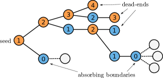
Imagine a cascading product like a meme, conspiracy theory, rumor, or a piece of software spreading in a population of agents. At every transmission step in the cascade, the product has the chance to independently improve with probability or get worse with probability . This process can stop for two reasons: either the quality of the product drops to zero, or the agents sharing it cannot find others to pass it on to (see Fig. 1).
As an example, consider open source projects where a seed piece of software is made available for others to fork and modify Nyman (2015). These modifications can either enhance or degrade the software, as well as its governance Viseur (2012); Gamalielsson and Lundell (2014). For instance, better code or governance might make the software more accessible and easier to adopt and update, while poorly written code or bad governance practices can make the software difficult to maintain, eventually leading to its abandonment Coelho and Valente (2017). As a result, the quality of the software varies with each iteration, demonstrating the flexible and evolving nature of this type of cascade.
As a final and very different example, we note that we originally conceived the self-reinforcing mechanism as a model of forest fires gaining intensity as they burn trees but losing intensity as they traverse gaps in forest cover Redner et al. (in preparation). We explore this idea that cascades can deviate from universal classes when they can be amplified or attenuated as they spread.
More generally, SRCs are a cascade perspective on killed branching random walks where certain results are known for its critical point in a continuous limit Kesten (1978) and bounds on its critical behavior in the discrete case Aidékon et al. (2013). Here, we provide an exact recursive solution, closed-form expressions for the expected cascade sizes and their critical point, and offer other new avenues of mathematical analyses. Beyond theoretical contributions, our results illustrate how diverse scaling exponents can easily be observed in cascades.
Recursive solution
Mathematically, we consider a general branching structure for contacts within the population. At any node, we define as the probability generating function for the number of “children” neighbors (occupied or not) of that node, being the probability of branching into exactly children Wilf (1994). The probability is equal to the probability that any node in the cascade is a dead-end without children, one of two ways for a chain of transmission to end. Importantly, and in line with recent empirical findings Gleeson et al. (2020), the branching number is drawn independently and identically at each node. However, considering generation- or intensity-dependent distributions for the branching number would be a straightforward extension of the model.
We pick the first node on this structure to start a cascade of intensity 1 (more generally, ). Any potential children will be either receptive to the process with probability , and continue the process with intensity 2; or non-receptive, such that they end their branch of the cascade by reaching intensity 0. In the next step, children with non-zero intensity in the last step (if any) can recruit their own receptive children (if any) to continue the process with intensity 3; or convince their non-receptive children (if any) to continue the process with intensity 1. In general, intensity increases when the cascade spreads to receptive nodes and decreases when it spreads to non-receptive ones. Any branch of the cascade dies either when it reaches a dead-end of the branching process or when its intensity goes to zero.
We can solve this process using a self-consistent recursive solution. Let be the probability generating function for the cascade size distribution of a node of intensity 1 Newman et al. (2001). Since the root node is part of the cascade, has to be proportional to to count that node. After that, every possible neighbor generated by is either receptive with probability , which increments the intensity by 1, or non-receptive with probability , in which case the neighbor does not continue the process as it reaches intensity 0. Neighbors of intensity 2 will lead to cascades whose size will be generated by and neighbors of intensity 0 will lead to trivial cascades of size 0, as generated by . We can therefore write to define a recursive self-consistent equation. In this equation, we use the fact that a cascade produced by a node of intensity is the sum of the cascades produced by its children, and that the probability generating function for the sum of a variable number of independent random variables is the composition of the probability generating functions.
More generally, we can write
| (1) |
to account for the fact that non-receptive nodes decrease the intensity but do not necessarily end the process if .
To solve Eq. (1), we follow the approach described in Sec. IIC of Ref. Newman et al. (2001) to iterate the recursive equations for a sample of values on the unit circle in the complex -plane , up to a certain maximal intensity (we use 100), until all values converge to within a certain precision threshold (we use ). Once a fixed point has been reached, we can extract which generates the cascade size distribution from the seed (assuming ). We can also obtain the probability that a cascade is supercritical and never ends as since supercritical cascades are of infinite size not accounted for in Eq. (1).
Critical point
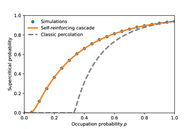
We first look at the phase transition of SRCs in Fig. 2. We assume that the number of children nodes is drawn from a Poisson distribution of mean . The self-intensifying mechanism greatly reduces the critical point of the process. For an average branching number , we find at instead of for the emergence of a giant connected component (infinite-size) cascade in a random networkMolloy and Reed (1995).
We now derive a closed-form solution for the critical point. To gain some insights into the expected behavior of Eq. (1), we rewrite the system as a recursion over the expected cascade size when starting at a node of intensity for a given . To calculate we take the derivative of and evaluate at (using the facts that this extracts the first moment from a probability generating function, and that and in the subcritical regime), to get
| (2) |
This non-homogeneous linear difference equation can be solved with initial conditions and . We obtain
| (3) |
We calculate the critical point of the process as the value of where the susceptibility of the system diverges, such that . We find
| (4) |
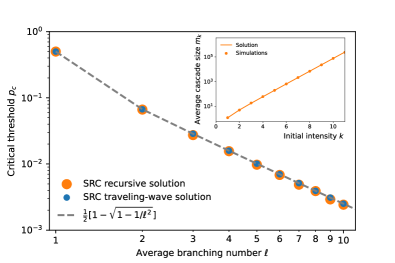
Figure 3 validates this explicit closed-form expression against our other solutions and compares our explicit solution for expected cascade size against simulations in the inset.
Extended critical behavior
To get a better intuition on the behavior of the system around the critical point, we rely on known results for extremal paths on trees Majumdar and Krapivsky (2000). Accordingly, we focus on the expected maximal number of positive steps in intensity (i.e., the number of receptive nodes met) along any paths after generations of the process with parameter . To solve for the dynamics of we define the cumulative probability , with initial condition . We can write a recursion similar to Eq. (1),
| (5) |
Based on previous work Majumdar and Krapivsky (2000), we use a traveling-wave Ansatz . We linearize Eq. (5) in the region far ahead of the front (; ) and look for an exponential solution, , to eventually find that the speed of the front relates to the decay exponent via the following transcendental equation
| (6) |
The first equality comes from the linearization of Eq. (5); the second one by solving for the minimum value of the corresponding speed, in accordance to the principle of velocity selection Majumdar and Krapivsky (2000).
The traveling-wave front means that, to first order, we have . Assuming we start at an intensity of , the expected maximal intensity after generations reads
| (7) |
since the process is expected to have reached receptive nodes that increased intensity by 1 and therefore non-receptive nodes that decreased intensity by 1. The expected maximal intensity should diverge for and go to zero for . The critical point is therefore defined by
| (8) |
One then finds by imposing the critical velocity, , in Eq. (6). This derivation yields the same solution as Eq. (4), as shown in Fig. 3.
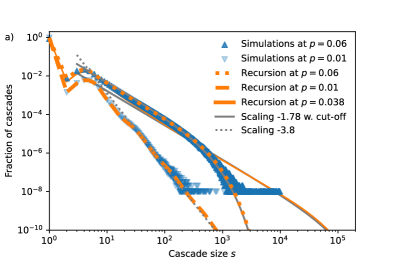
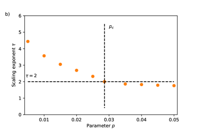
Figure 4 shows that below , the cascade size distributions of the SRC feature steep power-law tails with tunable scaling exponents . The exponent decreases when increases until reaching at , as required for the expected cascade size to diverge. For larger values of , we find that a robust power-law behavior with exponential cut-off exists well above .
Why do we find a critical-like scaling off the critical point? The presence of power-law tails in the subcritical regime has recently been proven in the context of killed branching random walks in Ref. Aidékon et al. (2013). In SRC, this likely occurs because we are looking at cascade size, which is exponentially related to cascade intensity as per Eq. (3), and intensity is related to cascade depth which is known to decay exponentially in the subcritical regimes Grimmett (1999). This combination of exponentials is a known mechanism to produce power-law tails Newman (2005).
To characterize the power-law behavior in the supercritical regime, we add the universal logarithmic correction to under the traveling-wave solution Bramson (1978); Brunet and Derrida (1997); Brunet (2016), which becomes . With this correction, the critical condition is
| (9) |
We thus find a critical generation number such that, in the supercritical regime , the expected maximal intensity only starts growing after some transient number of generations given by
| (10) |
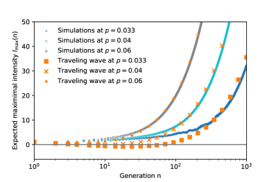
We expect a power-law behavior for cascades of size not larger than , the expected cascade size reachable by generation . If reaches , then , and the typical exponential behavior above the percolation threshold should be recovered. The critical generation thus imposes a critical cutoff at on the cascade size distribution. We estimate the cascade size to be distributed as a power-law with exponential cutoff . As Fig. 4(a) shows for , for which and , our estimation is in excellent agreement with the exact results from recursion. As the value of increases, decreases, and additional correction terms (first a non-universal term of order ) would eventually come into play to push the cut-off to higher values Brunet (2016). We illustrate this using in Fig. 4(a), where Eq. (10) predicts , yet we obtain a much better fit with the value used in the figure. Our estimated cutoff thus offers a lower bound, such that the scaling behavior is observed for supercritical values of higher than expected from .
Discussion
The self-reinforcing cascade process presents key features that makes it particularly appealing for modeling contagions observed in socio-technical systems. It is a parsimonious model to capture the fact that the strength of individual beliefs or the quality of products may vary and influence the ability of an individual to further transmit the cascade. This variability is aligned with real-world phenomena, where not all individuals or contents are equally influential in the transmission of ideas or behaviors. With this simple mechanism, the SRC model can produce a wide range of scaling behaviors for cascade size distributions, whereas classic percolation is constrained by a unique and universal scaling exponent obtained only at a precise critical point.
While self-similar or isotropic spreading rules are mathematically convenient, providing straightforward solutions and modeling frameworks, self-reinforcing cascades can offer advantages that warrant further study. The flexibility and richness of their outcome suggest that they are better suited to capture the complexities of real-world social contagions.
We outlined several important properties of self-reinforcing cascades and proposed three analytical approaches—exact probability generating functions, explicit solution of expected cascades, and the traveling-wave technique—to better understand these processes. This model may provide a useful framework for researchers and practitioners seeking to understand cascading behavior in complex real-world systems.
Acknowledgments
The authors acknowledge financial support from The National Science Foundation awards #2419733 (L.H.-D. and G.B.) and #2242829 (J.L. and G.B.) as well as from Science Foundation Ireland under Grant number 12/RC/2289 P2 (J.P.G).
References
- Notarmuzi et al. (2022) Daniele Notarmuzi, Claudio Castellano, Alessandro Flammini, Dario Mazzilli, and Filippo Radicchi, “Universality, criticality and complexity of information propagation in social media,” Nature Communications 13, 1308 (2022).
- Harris et al. (1963) Theodore Edward Harris et al., The theory of branching processes, Vol. 6 (Springer Berlin, 1963).
- Radicchi et al. (2020) Filippo Radicchi, Claudio Castellano, Alessandro Flammini, Miguel A Muñoz, and Daniele Notarmuzi, “Classes of critical avalanche dynamics in complex networks,” Physical Review Research 2, 033171 (2020).
- Nishi et al. (2016) Ryosuke Nishi, Taro Takaguchi, Keigo Oka, Takanori Maehara, Masashi Toyoda, Ken-ichi Kawarabayashi, and Naoki Masuda, “Reply trees in Twitter: data analysis and branching process models,” Social Network Analysis and Mining 6, 1–13 (2016).
- Wegrzycki et al. (2017) Karol Wegrzycki, Piotr Sankowski, Andrzej Pacuk, and Piotr Wygocki, “Why do cascade sizes follow a power-law?” in Proceedings of the 26th international conference on World Wide Web (2017) pp. 569–576.
- Nyman (2015) Linus Nyman, Understanding Code Forking in Open Source Software: An examination of code forking, its effect on open source software, and how it is viewed and practiced by developers (Hanken School of Economics, 2015).
- Viseur (2012) Robert Viseur, “Forks impacts and motivations in free and open source projects,” International Journal of Advanced Computer Science and Applications 3, 117–122 (2012).
- Gamalielsson and Lundell (2014) Jonas Gamalielsson and Björn Lundell, “Sustainability of open source software communities beyond a fork: How and why has the LibreOffice project evolved?” Journal of systems and Software 89, 128–145 (2014).
- Coelho and Valente (2017) Jailton Coelho and Marco Tulio Valente, “Why modern open source projects fail,” in Proceedings of the 2017 11th Joint meeting on foundations of software engineering (2017) pp. 186–196.
- Redner et al. (in preparation) S. Redner, L. Hébert-Dufresne, and P.L. Krapivsky, “Long-range fire propagation, working title,” (in preparation).
- Kesten (1978) Harry Kesten, “Branching brownian motion with absorption,” Stochastic Processes and their Applications 7, 9–47 (1978).
- Aidékon et al. (2013) EF Aidékon, Y Hu, and O Zindy, “The precise tail behavior of the total progeny of a killed branching random walk,” The Annals of Probability 41, 3786–3878 (2013).
- Wilf (1994) Herbert S. Wilf, Generating functionology (Academic Press, 1994).
- Gleeson et al. (2020) James P Gleeson, Tomokatsu Onaga, Peter Fennell, James Cotter, Raymond Burke, and David JP O’Sullivan, “Branching process descriptions of information cascades on Twitter,” Journal of Complex Networks 8, cnab002 (2020).
- Newman et al. (2001) M. E. J. Newman, S. H. Strogatz, and D. J. Watts, “Random graphs with arbitrary degree distributions and their applications,” Phys. Rev. E 64, 026118 (2001).
- Molloy and Reed (1995) Michael Molloy and Bruce Reed, “A critical point for random graphs with a given degree sequence,” Random structures & algorithms 6, 161–180 (1995).
- Majumdar and Krapivsky (2000) Satya N Majumdar and PL Krapivsky, “Extremal paths on a random Cayley tree,” Physical Review E 62, 7735 (2000).
- Grimmett (1999) Geoffrey Grimmett, Percolation (Springer, 1999).
- Newman (2005) M. E. J. Newman, “Power laws, Pareto distributions and Zipf’s law,” Contemporary Physics 46, 323–351 (2005).
- Bramson (1978) Maury D Bramson, “Maximal displacement of branching Brownian motion,” Communications on Pure and Applied Mathematics 31, 531–581 (1978).
- Brunet and Derrida (1997) Éric Brunet and Bernard Derrida, “Shift in the velocity of a front due to a cutoff,” Physical Review E 56, 2597 (1997).
- Brunet (2016) Éric Brunet, “Some aspects of the Fisher-KPP equation and the branching Brownian motion,” Habilitation à diriger des recherches, UPMC (2016).